SpaceX Starlink Dish Steers 540 Mbps Beams Without Moving Parts
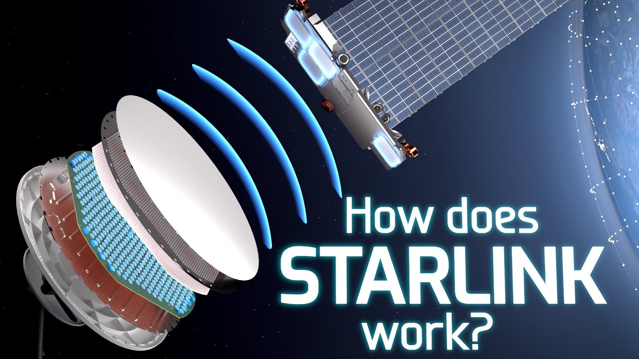
How does Starlink Satellite Internet Work?📡☄🖥 — Branch Education

Branch Education

By executing microsecond phase shifts across 1,280 printed patch antennas, the terminal achieves a 3,500-fold power gain and steers 64-QAM radio beams across 100 degrees to track orbital satellites without mechanical wear.

AI-assisted summary of How does Starlink Satellite Internet Work?📡☄🖥 — original source. Check the original for full context.

Source published:

Key ideas

  • Starlink achieves low-latency (~20 ms) broadband by deploying a mega-constellation of table-sized satellites at an altitude of 550 km in Low Earth Orbit traveling at 27,000 km/h, requiring handoffs to a new satellite every four minutes. (0:00)
  • The Dishy McFlatface terminal uses a 55 cm PCB containing 1,280 aperture-coupled patch antennas in a hexagonal lattice, generating an electronically steered beam with an effective radiated power gain roughly 3,500 times that of a single antenna. (12:45)
  • Beam steering across a 100-degree field of view is executed purely through solid-state phase shifts driven by 20 beamformer ICs and 640 front-end modules, completely avoiding rapid mechanical motor wear. (16:52)
  • High-throughput data encoding relies on 64-QAM running at 90 million 6-bit symbols per second, producing a gross 540 Mbps throughput asymmetrically allocated via time division (926 ms downlink vs. 74 ms uplink per second). (24:38)

Detailed notes

## Background Published on YouTube by Branch Education on August 19, 2022, this video explores the engineering behind Starlink satellite internet. According to the page description, it breaks down how a ground dish and a satellite orbiting 550 km above at 27,000 km/h establish a continuous link, form and steer data beams across the sky, and pack data within those beams for high-speed connectivity.

## TL;DR The video deconstructs SpaceX's Starlink system through the hardware of the 'Dishy McFlatface' ground terminal and its orbital counterpart. It explains how a 55-centimeter circuit board housing 1,280 aperture-coupled patch antennas uses wave superposition and constructive interference to focus radio energy into a tight beam that reaches Low Earth Orbit. The presentation then details how solid-state phased-array beam steering tracks fast-moving satellites across a 100-degree field of view without mechanical tracking motors. Finally, it outlines how 64-QAM modulation simultaneously manipulates carrier wave amplitude and phase to encode digital symbols, achieving raw data throughputs up to 540 Mbps.

## Atmosphere & style The presentation carries the polished, intellectually invigorating feel of high-end engineering education, blending intricate 3D architectural cutaways with precise technical exposition. Narrated with clear, enthusiastic authority by Phil Lee, the pacing balances dense physics with relatable visual metaphors—comparing microscopic antenna radiation to expanding balloons and light dimmers. Watching it feels like peering straight through solid aluminum and silicon into an invisible electromagnetic ballet, maintaining an underlying sense of marvel at the sheer precision required to connect Earth and orbit.

## Bulletin - [00:00](https://www.youtube.com/watch?v=qs2QcycggWU&t=0s) Starlink achieves low-latency (~20 ms) broadband by deploying a mega-constellation of table-sized satellites at an altitude of 550 km in Low Earth Orbit traveling at 27,000 km/h, requiring handoffs to a new satellite every four minutes. - [12:45](https://www.youtube.com/watch?v=qs2QcycggWU&t=765s) The Dishy McFlatface terminal uses a 55 cm PCB containing 1,280 aperture-coupled patch antennas in a hexagonal lattice, generating an electronically steered beam with an effective radiated power gain roughly 3,500 times that of a single antenna. - [16:52](https://www.youtube.com/watch?v=qs2QcycggWU&t=1012s) Beam steering across a 100-degree field of view is executed purely through solid-state phase shifts driven by 20 beamformer ICs and 640 front-end modules, completely avoiding rapid mechanical motor wear. - [24:38](https://www.youtube.com/watch?v=qs2QcycggWU&t=1478s) High-throughput data encoding relies on 64-QAM running at 90 million 6-bit symbols per second, producing a gross 540 Mbps throughput asymmetrically allocated via time division (926 ms downlink vs. 74 ms uplink per second).

## Key takeaways - [01:46](https://www.youtube.com/watch?v=qs2QcycggWU&t=106s) Unlike broadcast TV satellites at 35,000 km geostationary orbit that transmit wide, receive-only signals, Starlink operates bidirectional low Earth orbit satellites at 550 km to keep latency near 20 milliseconds. - [00:00](https://www.youtube.com/watch?v=qs2QcycggWU&t=0s) Because LEO satellites move across the sky at 27,000 km/h, the ground terminal must track them continuously and switch satellite connections roughly every four minutes. - [03:28](https://www.youtube.com/watch?v=qs2QcycggWU&t=208s) The internal motors inside Dishy McFlatface are only used for initial coarse alignment during setup; all real-time tracking is handled without moving parts via electronic beam steering. - [03:28](https://www.youtube.com/watch?v=qs2QcycggWU&t=208s) The terminal's 55 cm PCB integrates 1,280 aperture-coupled patch antennas arranged in a hexagonal honeycomb layout driven by 640 front-end modules and 20 larger beamformer microchips. - [05:06](https://www.youtube.com/watch?v=qs2QcycggWU&t=306s) Individual patch antennas operate at around 12 GHz, alternating charge across the copper disc every 42 picoseconds without direct physical contact with the underlying microstrip feedline. - [12:45](https://www.youtube.com/watch?v=qs2QcycggWU&t=765s) Constructive and destructive wave interference from the 1,280 antennas combines into a narrow, focused beam front yielding roughly 3,500 times the effective isotropic radiated power of a single antenna. - [16:52](https://www.youtube.com/watch?v=qs2QcycggWU&t=1012s) By calculating precise phase delays every few microseconds using onboard GPS and ephemeris tracking, the dish steers the constructive beam angle across a 100-degree field of view. - [21:11](https://www.youtube.com/watch?v=qs2QcycggWU&t=1271s) Starlink satellites deploy four distinct phased arrays: two dedicated to user terminals on the ground and two dedicated to gateway feeder links. - [22:24](https://www.youtube.com/watch?v=qs2QcycggWU&t=1344s) Data is encoded using 64-QAM modulation, where 6-bit symbols are mapped onto polar coordinates of carrier amplitude and phase shift lasting approximately 10 nanoseconds each. - [24:38](https://www.youtube.com/watch?v=qs2QcycggWU&t=1478s) Operating at 90 million symbols per second delivers 540 Mbps of raw throughput, which is split via time-division multiplexing into roughly 926 ms of downlink and 74 ms of uplink each second. - [26:02](https://www.youtube.com/watch?v=qs2QcycggWU&t=1562s) At a 2.5 cm wavelength, approximately 22 million wave cycles span the 550 km distance between the dish and the satellite, taking just 2 milliseconds to traverse the gap.

## Detailed walkthrough ### [00:00](https://www.youtube.com/watch?v=qs2QcycggWU&t=0s) Overview of Exploring Starlink

Setting up high-speed internet in the middle of nowhere using an oversized, pizza-shaped dish sitting on a roof to communicate with an orbital satellite is an astounding technical reality. As the narrator frames it:

> “Beaming internet from the middle of the woods using an extra-large pizza-sized satellite dish placed on top of your house up to a satellite orbiting 550 kilometers outside Earth’s atmosphere, well let’s be honest, is technologically mind-blowing.”

The technical challenge is magnified by extreme orbital dynamics. Starlink satellites travel at approximately 27,000 kilometers per hour in low Earth orbit. Despite that breakneck pace, the ground system and the satellites exchange hundreds of megabits per second of data by continuously angling and steering a focused data beam between them. Because each satellite moves across the sky so rapidly, the ground dish must hand over and switch to a different satellite roughly every four minutes when the current one leaves its line of sight.

To understand this system, the breakdown addresses three core pillars: 1. **Beam Generation:** How the ground terminal creates a focused beam of data capable of reaching space. 2. **Beam Steering:** How the dish steers that beam continuously across the sky without physically rotating to track the satellite. 3. **Data Encoding:** What data is packed inside the beam that allows an end user to seamlessly stream five high-definition movies or shows simultaneously.

Because the technical details are dense, the narrator playfully suggests viewing habits:

> “We recommend watching it first at one point two five times speed, and then a second time at one and a half speed to understand it as a complete technology.”

---

[01:46](https://www.youtube.com/watch?v=qs2QcycggWU&t=106s) Difference Between Starlink and Broadcast Satellites

To grasp how unique Starlink's terminal—dubbed "Dishy McFlatface" or simply "Dishy" by Elon Musk—truly is, it helps to contrast it with a conventional satellite television dish.

A standard television dish uses a curved parabolic reflector to bounce and focus incoming electromagnetic waves sent from geostationary broadcast satellites orbiting at an altitude of approximately 35,000 kilometers. These traditional TV dishes are strictly one-way receivers; they capture television broadcasts, but cannot transmit data back into space. Furthermore, the satellites transmitting these TV signals are van-sized platforms that cast wide, fan-like coverage footprints spanning entire continents (larger than North America).

Dishy, by contrast, functions as a bidirectional transceiver that both sends and receives high-throughput internet data to and from a satellite orbiting 550 kilometers above Earth. While 550 kilometers is roughly 60 times closer than geostationary orbit, it remains a vast distance over which to transmit a wireless signal. This proximity requires Dishy and the satellite to generate narrow, powerful, steered beams directed squarely at each other.

To deliver low-latency performance (around 20 milliseconds), which is vital for real-time web browsing and online gaming, Starlink satellites must operate in Low Earth Orbit (LEO). Operating in LEO means each table-sized satellite covers a much smaller geographic footprint. Consequently, maintaining unbroken global internet coverage requires a massive constellation of 10,000 or more fast-moving LEO satellites.

| Feature | Broadcast TV Satellite System | Starlink Satellite System | |:--- |:--- |:--- | | **Dish Operation** | Receive-only | Bidirectional (Transmit and Receive) | | **Orbit Altitude** | ~35,000 km (Geostationary) | ~550 km (Low Earth Orbit) | | **Latency** | High (hundreds of milliseconds) | Low (~20 milliseconds) | | **Beam Profile** | Wide fan footprint (continent-spanning) | Narrow, tight, steerable directed beams | | **Satellite Size** | Van-sized | Table-sized | | **Constellation Size** | Few stationary satellites | 10,000+ satellites orbiting at ~27,000 km/h |

---

[03:28](https://www.youtube.com/watch?v=qs2QcycggWU&t=208s) Parts Inside a Dishy McFlatface

Tearing down Dishy McFlatface reveals that the system is entirely distinct from a simple passive metal dish. At the rear housing, there are dual motors alongside an Ethernet cable connecting the unit to an indoor router. These motors are not designed to continuously track satellites across the sky; they engage solely during initial setup to orient the dish face in the correct general quadrant of the sky.

Beneath the shell lies an aluminum structural backplate supporting a massive printed circuit board (PCB): - **Rear of the PCB:** Populated by 640 small microchips and 20 larger microchips laid out in a geometric hierarchy, with intricate traces radiating outward from the larger chips to the smaller ones. Peripheral areas house support silicon, including a main CPU and a GPS module. - **Front of the PCB:** Surfaces roughly 1,400 copper circles separated by an isolating grid of squares. - **Upper Stack:** Layered above the PCB is a rubber honeycomb spacer containing small, notched copper discs, topped by a second honeycomb pattern that interfaces directly beneath the front radome face.

In total, this architecture comprises 1,280 individual antennas arranged in a hexagonal honeycomb layout. Each vertical stack of copper discs represents a single discrete antenna driven by the microchips on the PCB. Operating in unison, this assembly forms an electronically controlled phased array capable of forming and steering directional electromagnetic beams to a satellite 550 kilometers overhead without any mechanical movement.

```mermaid flowchart TD accTitle: Internal Layers of Dishy McFlatface accDescr: Cross-section from the rear motors through the PCB to the front honeycomb radome face.

subgraph Rear ["Base & Controls"] M["Motors (Initial pointing only)"] ETH["Ethernet to Router"] BP["Aluminum Structural Back-plate"] end

subgraph PCB ["Printed Circuit Board"] B_CHIPS["640 Small Chips + 20 Large Chips<br/>Main CPU & GPS Module"] F_CIRCLES["1,400ish Copper Circles with Isolation Grid"] end

subgraph Front ["Antenna Radiator Layers"] H1["Rubber Honeycomb + Notched Copper Discs"] H2["Secondary Honeycomb Pattern"] RAD["Dish Front Cover (Radome)"] end

Rear --> PCB --> Front ```

---

[05:06](https://www.youtube.com/watch?v=qs2QcycggWU&t=306s) How Does an Aperture-Coupled Patch Antenna Work?

Each individual antenna unit inside Dishy is an aperture-coupled patch antenna constructed from six distinct layers, the majority of which are integrated directly into the PCB stack. While vastly more complex than a traditional metal radio rod, its operation can be understood by looking at a simplified two-element model: a microstrip transmission feed line and an antenna patch.

At the bottom of the stack, a microstrip feed line—essentially a copper trace routed from one of the small front-end microchips—terminates abruptly beneath the antenna footprint. The chip drives this trace with a high-frequency alternating current signal operating at 12 GHz (12 billion cycles per second). At this frequency, the voltage alternates sinusoidally between positive and negative polarity every 42 picoseconds, completing a full cycle every 83 picoseconds.

High-frequency alternating current behaves differently from direct current or standard 50–60 Hz household utility electricity. Even though the notched copper circular patch suspended above the feed line has no direct physical contact with the wire, the signal couples across the gap: 1. **Negative Half-Cycle (Trough):** When the 12 GHz input voltage reaches its negative peak, an excess concentration of electrons gathers at the terminal tip of the feed wire. This negative charge repels the free electrons inside the overlying copper patch, driving them toward the opposite side of the circular disc. This charge migration polarizes the disc, creating a positive charge on near regions, a negative charge on far regions, and setting up an electric field between the feed line and the patch. 2. **Positive Half-Cycle (Peak):** Exactly 42 picoseconds later, the voltage inverts to its maximum positive potential. Electrons rush out of the tip of the feed trace, leaving a net positive charge. This draws the electrons in the antenna patch back across the disc to the opposite edge, flipping the voltage gradient across the disc and completely reversing the direction of the electric field.

Because the feed line continuously oscillates at 12 GHz, electrons rush back and forth across the patch, creating an alternating current and oscillating electric and magnetic fields.

---

[09:13](https://www.youtube.com/watch?v=qs2QcycggWU&t=553s) Electromagnetic Wave Emission

Analyzing the oscillating field geometry reveals how radiation breaks away into free space: - **Field Cancellation and Fringing Fields:** Resolving the electric field vectors across the patch shows that vertical components point in equal and opposite directions, canceling each other out. However, horizontal fields along the plane of the patch—known as fringing fields—point in the same direction and reinforce one another, producing a combined net electric field vector. - **Magnetic Field Generation:** Concurrently, the physical back-and-forth transit of electrons across the face of the copper disc forms an electric current. This alternating current induces a magnetic field whose vector is oriented perpendicular to the fringing electric field.

Because these electric and magnetic field vectors alternate cyclically and propagate outward perpendicular to one another, they launch an electromagnetic wave. Due to the natural curvature of the field lines across the disc, the radiating wave expands outward like a spherical balloon or the light spreading from an overhead bulb. Modulating the signal intensity is straightforward:

> “Which means, if we want to make these electric and magnetic fields stronger, we just have to increase the voltage sent to the feedline. It’s like a dimmer on a light switch: more power equals a brighter light.”

This antenna operates bidirectionally through reciprocity, though not simultaneously: - **Transmission:** The front-end module microchip injects the 12 GHz drive voltage into the feed trace, radiating outward. - **Reception:** The front-end module switches into receive mode, disabling the local 12 GHz transmitter. An incoming electromagnetic wave arriving from the satellite impinges on the copper patch, causing electrons within the metal to oscillate. This induced high-frequency signal couples back into the microstrip feedline, which routes it into the front-end module to be amplified.

In reality, the physical antenna inside Dishy McFlatface incorporates several additional layers: - Dual stacked circular patches: the lower patch handles transmission at 13 GHz, while the upper patch is tuned to receive downlink signals at 11.7 GHz. - Dual H-shaped aperture slots and dual feed lines to produce circular polarization. - A rear reflective ground plane and specialized isolation structures designed to prevent electromagnetic interference or cross-talk between neighboring array elements. - Strict mechanical dimensions designed to resonate exclusively at satellite frequencies, effectively filtering out the ambient sea of ambient electromagnetic waves—including sunlight, cell signals, and broadcast television—that continuously wash over the surface of the Earth.

[12:16](https://www.youtube.com/watch?v=qs2QcycggWU&t=736s) Forming a Beam That Reaches Space: Beamforming

Individual aperture-coupled patch antennas are sharply tuned circuits that transmit and receive exclusively across a narrow frequency band, essentially disregarding any frequencies outside that range. Because an individual patch antenna measures only roughly a centimeter in diameter, relying on just one to transmit data across hundreds of kilometers is an impossible challenge. As narrator Phil Lee colorfully illustrates, “This single antenna is only a centimeter or so in diameter and using only it would be like turning on and off one light bulb and trying to see it from the international space station.” To bridge that distance, the signal must be amplified thousands of times over and concentrated into a tight, razor-sharp beam of electromagnetic energy directed straight into orbit.

This transformation is handled by the primary printed circuit board inside Dishy McFlatface, which spans 55 centimeters across and hosts 1,280 identical patch antennas arranged in a dense hexagonal grid. Combining the output of these antennas into a single directional signal is a technique known as beamforming. When two antennas sit adjacent to one another, their outgoing electromagnetic waves spread out spherically, like expanding balloons. Because only a single electric field vector can exist at any given point in space, the oscillating fields overlap and combine:

```mermaid flowchart TD accTitle: Beamforming Wave Superposition accDescr: Diagram illustrating how overlapping electromagnetic waves combine constructively and destructively to shape a directed beam front.

subgraph Emission["Antenna Emission"] A1["Antenna 1: 12 GHz Wave"] A2["Antenna 2: 12 GHz Wave"] end

subgraph Superposition["Superposition in Free Space"] C["In-Phase Alignment<br/>Peaks align with peaks"] D["Out-of-Phase Alignment<br/>Peaks align with troughs"] end

subgraph Interference["Interference Results"] CI["Constructive Interference<br/>Amplitudes add together"] DI["Destructive Interference<br/>Amplitudes cancel out"] end

Out["Focused Beam Front<br/>~3500x effective power concentrated toward space"]

A1 --> C A1 --> D A2 --> C A2 --> D C --> CI D --> DI CI --> Out ```

Where the peaks and troughs align simultaneously in the same orientation, constructive interference reinforces the wave into a much narrower, brighter path. Where a peak encounters an opposing trough, destructive interference cancels the signal out entirely.

Scaling this behavior across all 1,280 antennas creates an intense, coherent beam front capable of punching through the atmosphere. The resulting power boost does not simply equal the sum of the components. Rather than producing 1,280 times the power of a lone antenna, the array yields an effective isotropic radiated power and reach roughly 3,500 times greater than a single element. By engineering destructive interference along the sides and constructive interference out front, the array acts as if 1,280 light bulbs were encased in reflective mirrors with only a single opening left open for the concentrated beam to escape.

- **Array dimensions:** 55 cm wide circular PCB with 1,280 antennas in a hexagonal lattice. - **Single antenna size:** Roughly 1 cm in diameter. - **Array amplification gain:** Roughly 3,500× effective power relative to a single patch antenna.

---

[15:15](https://www.youtube.com/watch?v=qs2QcycggWU&t=915s) Interlude: Engineering Skills and Brilliant Sponsorship

Deconstructing the internal mechanics of Dishy McFlatface and low Earth orbit satellite constellations highlights how modern hardware relies on cross-disciplinary knowledge spanning orbital mechanics, high-frequency electromagnetism, and complex signal processing. Lee notes that mastering these concepts requires moving past standard textbooks into interactive models, recommending Brilliant as an educational platform providing hands-on coursework in topics directly underpinning Starlink, such as Waves and Light and gravitational physics. For engineers and enthusiasts aiming to understand cutting-edge rocketry and communications hardware, Brilliant offers interactive lessons, with the first 200 sign-ups via `brilliant.org/brancheducation` receiving 20% off an annual subscription.

---

[16:52](https://www.youtube.com/watch?v=qs2QcycggWU&t=1012s) Steering a Beam Across the Sky: Phased Arrays

When all 1,280 antennas are fed an identical 12 GHz signal perfectly in sync, they produce a coherent beam radiating perpendicular to the face of the dish. However, a fixed beam cannot maintain an active internet connection with a Starlink satellite racing through low Earth orbit at 27,000 kilometers per hour. Relying on mechanical gimbals or motors to pivot the dish in real time to track the satellite is out of the question: “Using the motors isn’t feasible because they would break within a month and aren’t accurate enough.” Instead, the beam must be steered electronically with microsecond precision using phased array beam steering.

Understanding phase manipulation requires breaking down the core properties of a periodic radio wave: - **Amplitude:** The height or strength of the wave, adjusted by varying the electrical power supplied to the antenna. - **Frequency:** The count of wave cycles (peaks and troughs) cycling per second. - **Phase:** A horizontal time shift of the wave profile, measured in degrees from 0° to 359°, where a 360° shift represents one full cycle that resets back to the beginning.

```mermaid flowchart LR accTitle: Phased Array Beam Steering Signal Flow accDescr: Control architecture showing how Dishy computes orbital trajectories and distributes phase shifts to steer the radio beam electronically.

subgraph Tracking["Tracking Computations"] GPS["Onboard GPS Receiver"] Orbit["Satellite Ephemeris / Software Model"] Calc["Dishy Main Processor<br/>Calculates 3D steering angles every few μs"] end

subgraph Distribution["Silicon Control Hierarchy"] BF["20 Beamformer ICs"] FEM["640 Front-End Modules<br/>(32 FEMs per Beamformer)"] Ant["1,280 Patch Antennas<br/>(2 Antennas per FEM)"] end

GPS --> Calc Orbit --> Calc Calc -->|"Phase delay instructions"| BF BF --> FEM FEM --> Ant ```

By intentionally introducing progressive time delays—or phase shifts—between neighboring antennas, the peaks and troughs leave each patch at slightly staggered moments. As these staggered waves propagate outward, their line of constructive interference pivots off-center, pointing the main beam toward an angle rather than straight ahead. Continuously adjusting these phase values swings the constructive zone smoothly from left to right, functioning like a planar wave front hitting an angled coastline. Arranging the antennas across a two-dimensional surface extends this control across both azimuth and elevation, unlocking a total electronic steering field of view spanning 100 degrees without any physical movement.

Translating this theory into hardware requires continuous computation: - The dish matches its physical location (determined by an onboard GPS receiver) against the precise orbital positions of the Starlink constellation tracked in software. - The processor calculates the required 3D angles and solves the exact phase delay needed for all 1,280 antennas. - These phase-shift commands route to 20 central beamformer integrated circuits on the board. - Each beamformer controls 32 front-end modules (640 FEMs across the whole array), and each front-end module manages the feedlines for two individual antennas. - These calculations refresh every few microseconds, dynamically holding the beam locked onto the satellite as it traverses the sky.

---

[21:11](https://www.youtube.com/watch?v=qs2QcycggWU&t=1271s) Phased Array Trade-Offs and Deployments

Electronic beam steering is not without imperfections. The central concentration of energy is known as the main lobe, but because physical interference patterns never cancel out completely across all angles, secondary leakage paths form side lobes of lower power.

Phased arrays are also not unique to ground dishes. While Dishy McFlatface operates a single phased array, each Starlink satellite carries four distinct phased array panels: two dedicated to serving user terminals on the ground and two handling high-throughput feeder links back to dedicated ground stations. Similar solid-state electronically steered antennas are also deployed on commercial airliners to maintain mid-flight satellite internet connections without external moving domes.

Lee highlights the production effort behind visualizing these invisible wave interactions, noting that the animation and explanation required a month of engineering research, two dozen script revisions, and two months of 3D modeling and animation.

- **Main lobe vs. side lobes:** Constructive interference forms a primary high-power transmission beam, while slight interference mismatches bleed minimal energy into parasitic side lobes. - **Satellite payload antenna distribution:** Starlink satellites mount 4 independent phased arrays (2 downlinks for Dishy terminals, 2 feeder links for ground gateways). - **Steering envelope:** 100° total field of view achieved completely through solid-state phase adjustment.

---

[22:24](https://www.youtube.com/watch?v=qs2QcycggWU&t=1344s) Encoding High-Speed Data: Constellations and 64-QAM

Concentrating high-frequency, 12 GHz sinusoidal electromagnetic waves into a steerable beam provides the transmission pipe, but a simple sine wave carries no digital data by itself. Transforming continuous radio waves into binary code capable of streaming high-definition video requires modulation. Dishy McFlatface and Starlink satellites achieve this by manipulating both the amplitude and the phase of the carrier wave simultaneously, a technique known as 64-QAM (Quadrature Amplitude Modulation).

By varying both parameters together, engineers define distinct combinations where each unique pair of amplitude and phase corresponds to a specific sequence of binary bits:

| Parameter | 64-QAM Implementation Details | |:--- |:--- | | **Bits per Symbol** | 6 bits per discrete state ($2^6 = 64$ unique permutations) | | **State Mapping** | Constellation diagram utilizing polar coordinates | | **Radial Distance ($r$)** | Carrier wave amplitude (signal power / brightness level) | | **Angular Coordinate ($\theta$)** | Carrier wave phase shift relative to the reference signal | | **Symbol Duration** | Approximately 10 nanoseconds ($10 \text{ ns}$) | | **Wave Cycles per Symbol** | ~120 full sinusoidal wave periods at 12 GHz |

Visualizing this alphabet is done via a constellation diagram, which maps each 6-bit value onto a two-dimensional grid using polar coordinates: the distance from the center origin defines the signal’s amplitude, while the rotational angle measured counter-clockwise from the positive X-axis defines its phase shift.

For instance, to transmit the 6-bit string `011 101`, Dishy sets the carrier wave to 59% amplitude with a phase shift of 121 degrees. When the transmitter advances to the next 6-bit group, such as `101 000`, the radio hardware switches the signal to 87% amplitude and adjusts the phase angle to 305 degrees. Each of these discrete 6-bit packets is known as a symbol.

Every symbol is broadcast for roughly 10 nanoseconds before switching to the next state. Because a 12 GHz electromagnetic wave completes a full cycle once every 83 picoseconds, each 10-nanosecond symbol contains roughly 120 continuous wave cycles before the transmitter shifts to the next amplitude and phase setting.

[24:38](https://www.youtube.com/watch?v=qs2QcycggWU&t=1478s) High-Speed Data Rates and 64-QAM Modulation

Because phase and amplitude shifts occur across pico- and nanosecond scales, the system can pack roughly 90 million 6-bit groups—known as symbols—into every single second. This translates directly to an raw throughput of 540 million bits per second (540 Mbps). However, this total pipe must be divided between downloading and uploading. The patch antenna hardware cannot transmit and receive simultaneously, meaning it relies on time-division multiplexing: approximately 74 milliseconds out of every second are dedicated to Dishy transmitting data up to the Starlink satellite, while the remaining 926 milliseconds are reserved for the satellite transmitting data down to the user. Rather than clustering these blocks into large, contiguous chunks, the upload and download slots are finely interleaved throughout the second to minimize perceived latency.

The underlying mechanism of encoding 6-bit values through variations of amplitude and phase shifts is known as 64-QAM (Quadrature Amplitude Modulation). As the narrator notes: “This technique of sending 6-bit values using different variations of amplitude and phase is called 64QAM or Quadrature Amplitude Modulation and is more complicated than we discussed but let’s not get sidetracked.” Once these millions of 6-bit symbols stream across the sky to yield hundreds of megabits per second, digital media formats like H.264 (Advanced Video Coding) compress and decode the raw bits so they can ultimately render as smooth television shows and streaming video on user devices.

```mermaid flowchart TD accTitle: 64QAM Data Transmission and Time Division accDescr: Diagram illustrating 64QAM symbol generation yielding 540 Mbps, followed by asymmetric time division between upload and download.

subgraph SymGen["Modulation"] A["6-bit Symbols<br/>(90 Million/sec)"] -->|"64-QAM Modulation"| B["Raw Throughput<br/>(540 Mbps)"] end

subgraph TimeDiv["1-Second Time Allocation"] B --> C{"Time Division Multiplexing"} C -->|"74 ms / sec"| D["Uplink<br/>(Dishy to Satellite)"] C -->|"926 ms / sec"| E["Downlink<br/>(Satellite to Dishy)"] end

subgraph Delivery["End User Application"] E --> F["H.264 Video Decoder"] F --> G["Streaming Video Playback"] end ```

- **Symbol Rate:** 90 million 6-bit symbols per second. - **Gross Data Rate:** 540 Mbps total bandwidth split dynamically across the link. - **Upload Allocation:** Roughly 74 ms per second allocated to Dishy uplink transmissions. - **Download Allocation:** Roughly 926 ms per second allocated to satellite downlink traffic. - **Latency Optimization:** Transmission time slots are chopped up and scattered throughout each second rather than grouped into monolithic blocks.

---

[26:02](https://www.youtube.com/watch?v=qs2QcycggWU&t=1562s) Scale, Speed, and Operational Realities

To present these complex concepts visually, the animations rely on severe compromises in scale that diverge significantly from physical reality. The narrator cautions: “First, the scale of practically everything in this video is off.” While Dishy McFlatface and the Starlink satellite can be rendered side by side at an accurate relative size, Dishy is physically separated from the satellite by an orbital distance of 550 kilometers. Furthermore, the true electromagnetic waves emitted by the antenna have a wavelength of approximately 2.5 centimeters. Across that 550-kilometer gap, there are roughly 22 million distinct wavelengths stretching between the dish and the spacecraft, far exceeding the handful of waves visualized on screen. The true speed of propagation is virtually instantaneous to human perception: it takes an electromagnetic wave only about 2 milliseconds to travel the entire path between Dishy and the satellite.

A second critical visual liberty is the direction of transmission shown throughout the presentation. The animation disproportionately depicts Dishy radiating waves outward and sending data into orbit. In everyday practical use, Dishy operates far more frequently in receive mode, listening to data beamed down from space. The physical processes and underlying wave mechanics required to receive an incoming electromagnetic signal mirror those used to transmit one, functioning entirely in reverse.

- **Orbital Distance:** Dishy operates roughly 550 kilometers away from the satellite overhead. - **Signal Wavelength:** The emitted electromagnetic waves measure approximately 2.5 centimeters apart. - **Wave Quantity:** There are roughly 22 million discrete wavelengths spanning the space between Dishy and the satellite at any given moment. - **Transit Time:** Electromagnetic waves take only about 2 milliseconds to traverse the 550 km distance. - **Primary Operating Mode:** Dishy spends the overwhelming majority of its operational cycles receiving incoming downlink signals rather than emitting uplink signals.

---

[27:19](https://www.youtube.com/watch?v=qs2QcycggWU&t=1639s) Production Details and Credits

The narrator wraps up the deep dive by revealing that the initial script for the project ran over 45 minutes long. Rather than abandoning the cut content entirely, the excised technical nuances were preserved within the video's English (Canada) subtitles as creator comments. The episode concludes with acknowledgments to community supporters across Patreon and YouTube Memberships, along with special thanks directed to Colin O’Flynn at NewAE Technology, who supplied an actual Starlink Dishy printed circuit board (PCB) to enable high-detail imaging, physical teardowns, and engineering research for Branch Education's 3D animation work.

## Notable quotes > [00:00](https://www.youtube.com/watch?v=qs2QcycggWU&t=0s) Beaming internet from the middle of the woods using an extra-large pizza-sized satellite dish placed on top of your house up to a satellite orbiting 550 kilometers outside Earth’s atmosphere, well let’s be honest, is technologically mind-blowing.

## Mentioned Starlink, SpaceX, Dishy McFlatface, Elon Musk, Branch Education, Teddy Tablante, Phil Lee, Brilliant, Colin O’Flynn, NewAE Technology, Paul S., Prakash Kakadiya, Mike Radjabov, David Pinete, Raúl Núñez, Luis Huesca, Luis Zuleta, Blender, Adobe Premiere Pro, FCC, International Space Station

## Video description Go to http://brilliant.org/BranchEducation/ to sign up for free and expand your knowledge. The first 200 people will get 20% off their annual premium membership. With Starlink internet, data is continuously being sent between a ground dish and a Starlink satellite orbiting 550km above. Furthermore, the Starlink satellite zooms across the sky at 27,000km/hr! How can the dish and satellite maintain a continuous connection? And then how is data sent back and forth? Well, in this video we're going to dive into the inner workings for the ground dish and Starlink satellites, and see how a beam of data is formed, how this beam is swept across the sky, and then finally what exactly is in that beam that allows for incredibly fast internet! This is an incredible feat of technology and engineering, so stick around!

Do you want to support in-depth engineering and technology education? Support us on: https://www.patreon.com/brancheducation

Website: https://www.branch.education On Facebook: https://www.facebook.com/BranchEducation/ On Twitter: https://twitter.com/TeddyTablante On Insta: https://www.instagram.com/brancheducation/

Table of Contents: 00:00 - Intro to Starlink 01:00 - Overview of Exploring Starlink 01:46 - Difference between Starlink and Broadcast Satellites 03:28 - Parts Inside a Dishy McFlatface 05:06 - How does an Aperture Couple Patch Antenna Work? 09:13 - Electromagnetic Wave Emission 12:45 - Forming a Beam that Reaches Space: Beamforming 15:22 - Brilliant 16:52 - Steering a Beam to Sweep Across the Sky 18:54 - Starlink: Phase Array Beam Steering 21:11 - Notes on Phased Array Beam Steering 22:24 - Sending Data in a Beam to the Starlink Satellite 23:27 - Innerworkings of 64QAM 26:02 - Actual Size of Starlink Dishy & EM Waves 26:55 - Images from the Starlink Patent 27:49 - Outro

Key Branches from this video are: How does Bluetooth Work?

Erratum: At 2m50s, the orbits are inaccurate. The TV satellite should be in geostationary orbit moving in the same direction as the Earth. Furthermore, all the Starlink satellites should be orbiting West to East. Credit to Paul S.

Script, Modeling, Animation: Teddy Tablante Twitter: @teddytablante Modeling: Prakash Kakadiya Animation: Mike Radjabov Voice Over: Phil Lee Sound Design: www.drilu.mx Sound Effects: Luis Zuleta Sound Effects and Music Editor: David Pinete Sound Effects: Raúl Núñez Supervising Sound Editor and Mixer: Luis Huesca

Animation built using Blender 3.1.2 https://www.blender.org/ Post with Adobe Premiere Pro

References: Antenna Theory: https://www.antenna-theory.com/

Distributed Phase Shifter Array System and Method [Starlink Patent] https://patents.google.com/patent/US20180241122A1/en)..

Elon Musk's Starlink and Satellite Broadband https://dgtlinfra.com/elon-musk-starlink-and-satellite-broadband/

SpaceX Filings with FCC https://fcc.report/IBFS/Company/Space-Exploration-Technologies-Corp-SpaceX

SpaceX Reveals More Starlink Info After Launch of First 60 Satellites https://techcrunch.com/2019/05/24/spacex-reveals-more-starlink-info-after-launch-of-first-60-satellites/

Wikipedia contributors. "Antenna Types","Aperture(Antenna)" ,"Low Earth Orbit", "Patch Antenna", "Phased Array", "Starlink" Wikipedia, The Free Encyclopedia. Wikipedia, The Free Encyclopedia, Visited August 2022

#Starlink #Satellite #Internet

[Source](https://www.youtube.com/watch?v=qs2QcycggWU)

中文简报

SpaceX星链天线无机械运动部件即可操纵540 Mbps波束 通过在1,280个印刷微带贴片天线上执行微秒级相移,该终端实现了3,500倍的功率增益,并能在100度范围内偏转64-QAM无线电波束以跟踪轨道卫星,全程无机械磨损。 本视频通过“Dishy McFlatface”地面终端及其轨道对应设备的硬件,对SpaceX的星链系统进行了深度解析。视频解释了一块容纳1,280个孔径耦合贴片天线的55厘米电路板如何利用波的叠加与相长干涉,将无线电能量聚焦成可抵达近地轨道的狭窄波束。随后,演示详细说明了固态相控阵波束控制如何在无需机械跟踪电机的情况下,在100度的视场范围内跟踪快速移动的卫星。最后,视频概述了64-QAM调制如何通过同时操纵载波振幅与相位来编码数字符号,从而实现高达540 Mbps的原始数据吞吐量。 星链通过在550公里高度的近地轨道部署以27,000公里/小时运行的桌面大小巨型卫星星座,实现低延迟(约20毫秒)宽带,且每四分钟需要切换一次新卫星。 (0:00) Dishy McFlatface终端采用一块55厘米的PCB板,上面呈六边形晶格排列着1,280个孔径耦合贴片天线,产生电子操纵波束,其有效全向辐射功率增益约为单个天线的3,500倍。 (12:45) 跨越100度视场的波束操纵完全由20个波束成形IC和640个前端模块驱动的固态相移实现,彻底避免了机械电机的快速磨损。 (16:52) 高吞吐量数据编码依赖于以每秒9000万个6比特符号运行的64-QAM,产生540 Mbps的总吞吐量,并通过时分进行非对称分配(每秒下行926毫秒,上行74毫秒)。 (24:38)

Reading summary

Branch Education details how Starlink delivers high-speed broadband by pairing a massive Low Earth Orbit constellation with a solid-state phased-array ground terminal that forms, steers, and modulates microwave beams entirely electronically. Low Earth Orbit Network Architecture (1:46) Traditional satellite internet relies on van-sized broadcast satellites in geostationary orbit roughly 35,000 kilometers away, which produce continent-wide footprints, suffer high latency of hundreds of milliseconds, and communicate with passive, receive-only parabolic dishes. Starlink instead places table-sized satellites into Low Earth Orbit at approximately 550 kilometers altitude. Operating roughly 60 times closer to Earth reduces latency to around 20 milliseconds, which is critical for real-time applications. Because LEO satellites orbit at approximately 27,000 kilometers per hour, each spacecraft covers a smaller geographic footprint and remains in view for only about four minutes before passing beyond the horizon. Maintaining an unbroken connection requires a constellation of 10,000 or more satellites and bidirectional, highly focused beams exchanged between the orbital spacecraft and the user terminal. Aperture-Coupled Patches and Array Beamforming (5:06) The user terminal, known as Dishy McFlatface, houses 1,280 aperture-coupled patch antennas arranged in a hexagonal lattice across a 55-centimeter printed circuit board. Rather than relying on direct electrical contact, each antenna couples energy across an internal gap: high-frequency alternating current operating at 12 GHz oscillates electrons across stacked copper discs every 42 picoseconds. This movement generates reinforcing horizontal fringing electric fields and perpendicular magnetic fields that radiate outward as electromagnetic waves. A single patch antenna measures roughly one centimeter across and lacks the power to reach space. By synchronizing all 1,280 antennas, the array uses wave superposition to concentrate radiation. Outgoing waves reinforce each other through constructive interference in the forward direction while canceling out sideways via destructive interference. This beamforming process yields an effective isotropic radiated power roughly 3,500 times greater than that of a standalone antenna element. Phased-Array Electronic Beam Steering (16:52) To track satellites moving at 27,000 kilometers per hour, the terminal steers its transmission beam electronically across a 100-degree field of view rather than using mechanical gimbals, which would wear out quickly and lack precision. Dual rear motors are engaged solely during setup to align the dish toward the appropriate quadrant of the sky. Solid-state steering is achieved by applying phase shifts—staggered time delays—to the signals driving adjacent antennas, which tilts the plane of constructive interference. Dishy's main processor matches its onboard GPS coordinates against orbital ephemeris data, recalculating the necessary 3D angles every few microseconds. These commands route through 20 beamformer integrated circuits, which regulate 640 front-end modules driving the dual-feed patch elements to maintain an active link as the satellite traverses overhead. Data Modulation and Time-Division Allocation (22:24) To pack digital data onto the 12 GHz carrier wave, the system employs 64-QAM (Quadrature Amplitude Modulation). By concurrently varying the wave's amplitude and phase across 64 unique states mapped on a polar constellation diagram, each transmission symbol conveys a unique 6-bit value. Each symbol lasts approximately 10 nanoseconds, encompassing about 120 wave cycles. Broadcasting roughly 90 million symbols per second generates a raw bandwidth of 540 megabits per second. Because the patch antennas operate bidirectionally through reciprocity but cannot transmit and receive simultaneously, the link relies on time-division multiplexing: roughly 74 milliseconds per second are allocated for user uplink, while 926 milliseconds are dedicated to satellite downlink. Rather than occurring in single blocks, these upload and download slots are finely interleaved across each second to minimize perceived latency. The presentation notes that conceptual diagrams severely compress physical reality: across the 550-kilometer gap, roughly 22 million discrete 2.5-centimeter wavelengths stretch between the dish and the satellite, taking an electromagnetic wave approximately 2 milliseconds to traverse. In daily use, Dishy operates primarily in receive mode rather than transmitting, executing the same electromagnetic wave mechanics in reverse.

精炼阅读摘要

Branch Education 剖析了 Starlink 卫星互联网的技术实现机制,指出该系统依靠地面终端与近地轨道卫星之间的双向通信,利用包含 1280 个微带贴片天线的全电子相控阵、微秒级相位调控波束成形以及 64-QAM 高阶调制,在消除机械转动磨损的同时实现了高带宽、低延迟的稳定无线传输。 低轨卫星网络与传统卫星广播差异 (1:46) Branch Education 指出,传统卫星电视系统依赖位于约 35,000 公里地球静止轨道的巨型卫星,天线为单向被动接收,发射覆盖整个大陆的宽波束,通信延迟高达数百毫秒。与之相对,Starlink 地面终端“Dishy McFlatface”则是双向收发器,需与约 550 公里高度的近地轨道(LEO)卫星建立通信。尽管 550 公里高度将延迟大幅缩短至约 20 毫秒,但单颗卫星的地面覆盖范围显著减小,必须依赖超过 10,000 颗卫星组成庞大星座来维持无缝覆盖。 由于近地轨道卫星以每小时约 27,000 公里的极高速度飞行,单颗卫星掠过地面终端视野的时间仅有约 4 分钟。为了在这种高速相对运动中维持数百兆比特每秒(Mbps)的高速吞吐,地面终端与卫星之间不能使用泛波束,而必须生成窄小、高强度且持续对准彼此的定向波束,并在卫星移出视野时迅速切换交接至下一颗卫星。 终端硬件层级与贴片天线辐射原理 (3:28) 拆解 Dishy 内部构造可见,其底座配备的双电机仅在初次安装时用于将天线对准特定天空象限,日常跟踪并无机械转动。天线核心是一块直径 55 厘米的印刷电路板(PCB),其背面集成了 640 个小型前端模块(FEM)、20 个大型波束成形芯片、主中央处理器与 GPS 模块;正面则通过双层蜂窝结构与铜盘叠层,构成了 1,280 个呈六边形蜂窝排列的孔径耦合微带贴片天线。每个独立天线直径仅约 1 厘米,分层调谐至 13 GHz 发射与 11.7 GHz 接收频段,并利用双馈线与 H 型孔径产生圆极化波,有效阻隔日光和日常广播信号的干扰。 在微观辐射机制上,微带馈线由芯片驱动输入 12 GHz 的高频交流电,端点电压每 42 皮秒在正负极性间振荡一次。虽然铜盘与馈线无物理接触,但高频交变电场通过空间电容耦合引发铜盘表面电子来回迁移,其边缘电场与感应磁场垂直叠加并脱离天线向外发射球面电磁波。基于天线互易性,当卫星下行信号照射到铜盘时,会在金属中诱发相同振荡并耦合回馈线,经前端芯片放大后完成接收,不过发射与接收模式由开关分时控制,无法同时进行。 电磁波相干叠加与全电子波束转向 (12:16) 单个贴片天线尺寸仅约 1 厘米,其发出的微弱球面波无法独自跨越数百公里太空。Dishy 采用波束成形技术,将 1,280 个天线排布于阵列中同步辐射 12 GHz 电磁波。重叠波束在空间中发生干涉:波峰与波峰相遇的相长干涉使能量高度汇聚,波峰与波谷相遇的相消干涉则消除侧向信号,最终将整体有效全向辐射功率提升至单一天线的约 3,500 倍,聚合成一道刺破大气层的极窄主波束。 为了持续追踪高速划过天空的卫星,设备彻底舍弃了极易在数月内磨损损坏的机械旋转云台,完全依赖微秒级相控阵全电子波束转向。终端处理器结合板载 GPS 定位与软件中的卫星轨道星历,每隔数微秒计算出三维目标角度,并通过 20 块波束成形芯片向 640 个前端模块分发纳秒级别的渐进相位延迟指令。各天线单元出射波阵面的微小时间差使相长干涉轴线整体偏转,从而在静止的硬件形态下实现了宽达 100 度的全电子立体扫描视场。 64-QAM 符号编码与非对称时分复用 (22:24) 12 GHz 纯正弦波本身无法承载数据,系统采用 64-QAM(正交振幅调制)技术同时调制载波的振幅与相位。在极坐标星座图中,振幅代表信号强度,相位代表相对偏移角度,两者组合出 64 种离散物理状态,每个状态对应一组 6 比特的二进制符号。每个符号仅持续约 10 纳秒(对应约 120 个完整的 12 GHz 正弦波周期),使得系统每秒能向空间传输约 9,000 万个符号,实现高达 540 Mbps 的原始物理数据速率。 由于贴片天线硬件限制无法实现同频全双工收发,Dishy 采用了精细的时分多路复用(TDM)方案。在每一秒内,约 74 毫秒分配给地面终端向上发射数据,其余 926 毫秒则全部保留给卫星向下传输数据。为了消除网络交互延迟感,上行与下行时隙并非整块划分,而是被打碎并高度交错分布于每秒的时间轴中,最终下行比特流再经由 H.264 等压缩标准解码呈现为高清流媒体。 物理波长尺度与工程运行客观现实 (26:02) Branch Education 强调,视频演示为了教学可视化对物理尺度进行了必要简化。在现实中,地面终端与卫星相距 550 公里,而 12 GHz 信号的物理波长仅有约 2.5 厘米,这意味着地面与卫星之间在任意瞬时都容纳着约 2,200 万个连续波长,且电磁波跨越这段距离的单程传播时间仅需约 2 毫秒。 此外,终端日常运行绝大多数时间处于被动接收状态,而非动画中重点呈现的向外发射状态。同时,相控阵天线在物理上无法做到全角度完美抵消,除了中心高功率主瓣外,外围仍会伴随少许副瓣能量泄漏;而空间段的每颗 Starlink 卫星也均搭载了 4 块独立的相控阵面板(2 块服务地面终端,2 块连接地面网关站),以维持全天候天地通信链路的稳定运转。 Branch Education 指出,Starlink 成功将原先局限于航天与尖端军工的高频微波相控阵技术降本普及到了消费级硬件,但演示模型对电磁波传播与调制过程作了高度几何化提纯;在实际应用中,相控阵无法完全避免寄生副瓣泄露,且该系统的全球连通性与极低延迟表现,在根本上依赖于上万颗低轨卫星星座的庞大发射规模与高密度在轨交接。

Detailed notes — zh

## Background 本内容由 YouTube 科普频道 Branch Education 于 2022 年 8 月 19 日发布。视频深入拆解了 SpaceX 的星链(Starlink)卫星互联网系统,详细解释地面终端与在 550 公里高空以 27,000 km/h 飞行的卫星之间如何通过电磁波束形成、无机械偏转追踪以及高速数据编码来维持稳定连接。 ## TL;DR 视频系统性地剖析了星链系统的底层运作原理与工程架构。首先对比了传统高轨广播卫星与低轨星链在延迟、波束形态及双向传输上的本质区别,随后拆解了名为“Dishy McFlatface”的地面终端,展示其由 1280 个孔径耦合微带贴片天线构成的六边形相控阵列。接着深入解释了高频微带天线的电磁耦合与辐射机理,以及阵列如何通过相长干涉将等效功率放大近 3500 倍;最后详述了通过微秒级分布式芯片调相实现 100° 视场无机械波束转向,并结合 64QAM 调制与时分双工机制达成高达数百兆每秒的高速数据吞吐。 ## Atmosphere & style 整部影片呈现出一种极其严谨、沉稳且具有极高信息密度的工业级硬核科普质感。叙述者 Phil Lee 的嗓音清晰平稳、逻辑环环相扣,配合精美绝伦的 Blender 三维透视与微观切片动画,将原本抽象隐形的麦克斯韦电磁场与皮秒级电子震颤具象化为肉眼可见的空间波前。观看过程如同拆解一台精密复杂的现代工程仪器,在剥除层层技术外壳后,带给观众一种对尖端现代工程造物由衷的震撼与智力满足感。 ## Bulletin - [00:00](https://www.youtube.com/watch?v=qs2QcycggWU&t=0s) 星链通过运行在 550 公里低地球轨道(LEO)的巨型卫星星座,以约 27,000 km/h 的超高移速维持数百 Mbps 通信,将网络延迟大幅压缩至约 20 毫秒,且地面终端每隔约 4 分钟需无缝切换一次追踪卫星。 - [12:16](https://www.youtube.com/watch?v=qs2QcycggWU&t=736s) 星链地面终端 Dishy McFlatface 直径 55 厘米的 PCB 上集成了 1,280 个孔径耦合微带贴片天线,利用相长与相消干涉实现波束赋形,形成主波束有效功率达单天线约 3,500 倍的高定向窄波束。 - [16:52](https://www.youtube.com/watch?v=qs2QcycggWU&t=1012s) Dishy 彻底抛弃机械伺服持续追踪,依靠 20 颗波束赋形芯片与 640 颗射频前端芯片每隔几微秒动态重算各天线相位差,在无需任何机械转动的情况下实现 100° 视场内的电子相控阵波束转向。 - [22:24](https://www.youtube.com/watch?v=qs2QcycggWU&t=1344s) 数据通信采用 12 GHz Ku 频段与 64QAM 调制,每个 10 纳秒符号携带 6 比特信息,并结合时分双工(TDD)以每秒 74 毫秒上行、926 毫秒下行的交错切片架构实现高达 540 Mbps 的理论数据吞吐。 ## Key takeaways - [01:46](https://www.youtube.com/watch?v=qs2QcycggWU&t=106s) 星链选择 550 公里低地球轨道相较于传统 35,000 公里静止轨道卫星,将通信延迟从 600 毫秒以上降至约 20 毫秒,但需要发射上万颗卫星组成巨型星座以实现全球无死角覆盖。 - [01:46](https://www.youtube.com/watch?v=qs2QcycggWU&t=106s) 传统电视卫星锅为单向大范围广播接收天线,而星链 Dishy 必须实现双向高带宽数据互传,能量需收束为高增益窄波束动态精准对准太空。 - [03:28](https://www.youtube.com/watch?v=qs2QcycggWU&t=208s) Dishy 底部的步进电机仅用于初次通电时的粗略朝向校准,正常运行时的天际追踪完全不依赖机械旋转,避免了高频机械磨损故障。 - [05:07](https://www.youtube.com/watch?v=qs2QcycggWU&t=307s) 单天线单元采用六层孔径耦合微带贴片结构,射频芯片在底部馈电微带线上激励 12 GHz 正弦电压,通过每 42 皮秒正负交替的电场隔空耦合驱动贴片电子振荡。 - [09:13](https://www.youtube.com/watch?v=qs2QcycggWU&t=553s) 贴片边缘散逸的边缘电场与振荡电流诱发的交变磁场相互垂直,形成向外以光速膨胀辐射的 12 GHz 电磁波;天线硬件通过双层贴片分别匹配约 13 GHz 上行与 11.7 GHz 下行。 - [12:16](https://www.youtube.com/watch?v=qs2QcycggWU&t=736s) 单根直径约 1 厘米的贴片天线辐射极弱,1,280 个天线单元通过相长干涉(同相叠加增强)与相消干涉(异相抵消抑制)完成波束赋形,使合成主波束有效功率提升至单天线的近 3,500 倍。 - [16:52](https://www.youtube.com/watch?v=qs2QcycggWU&t=1012s) 相控阵波束转向技术通过在 0° 至 359° 范围内连续调整各个天线信号的发射相位差,使合成波前发生倾斜,从而在 100° 视场内实现全电子波束快速转向并锁定高速飞行的卫星。 - [20:14](https://www.youtube.com/watch?v=qs2QcycggWU&t=1214s) 地面终端采用分布式微芯片控制体系:主控通过 GPS 与轨道推算每隔数微秒下发指向参数,由 20 颗大型波束赋形芯片分发至 640 颗前端射频芯片,每颗芯片精准驱动 2 根贴片天线。 - [21:11](https://www.youtube.com/watch?v=qs2QcycggWU&t=1271s) 星链卫星单星搭载了 4 个相控阵天线,其中 2 个用于服务地面用户终端 Dishy,另外 2 个作为高速回传馈源对接地面骨干网关站。 - [22:24](https://www.youtube.com/watch?v=qs2QcycggWU&t=1344s) 星链采用 64QAM 调制方案,利用振幅与相位的 64 种独立组合将 6 位二进制数据映射为单符号,每个符号在空中持续约 10 纳秒并包含约 120 个完整的载波波长。 - [24:38](https://www.youtube.com/watch?v=qs2QcycggWU&t=1478s) 由于天线无法收发并行,系统采用时分双工(TDD)分配:每秒中约 74 毫秒用于终端上行,926 毫秒用于卫星下行,且时间切片均匀打散以保证极低的实时网络延迟。 - [26:02](https://www.youtube.com/watch?v=qs2QcycggWU&t=1562s) 在现实物理尺度上,12 GHz 电磁波波长仅约 2.5 厘米,地空 550 公里路径上密布约 2,200 万个波长,单向光速传播时间仅需约 2 毫秒。 ## Detailed walkthrough ### [00:00](https://www.youtube.com/watch?v=qs2QcycggWU&t=0s) 星链卫星互联网的惊人挑战与技术概览 身处偏僻森林,仅凭屋顶上一个特大号披萨大小的卫星天线,就能与远在地球大气层外 550 公里轨道上疾驰的卫星实现高速联网,这在工程技术层面令人惊叹。更不可思议的是,星链(Starlink)卫星在太空中的飞行速度高达每小时约 27,000 公里,而地面天线与卫星之间却能在两者以极快速度相对运动的同时,以数百兆比特每秒(hundreds of megabits per second)的速率持续收发数据。为了维持这种连接,地面天线与卫星必须毫不停歇地动态调整并偏转彼此之间的数据波束,精准地相互对准。不仅如此,由于单颗卫星很快就会飞离天线的视野范围,地面天线大约每隔 4 分钟就必须在不同的卫星之间完成一次无缝切换。 为了揭开这一套看似“魔法”般运作的系统,整个技术体系被拆解为三个核心支点:首先,拆解地面卫星天线内部,探究它是如何生成能够直达太空的高能数据波束;其次,解析天线如何在完全不依赖机械转动的情况下,实时偏转波束来追踪划过天空的高速卫星;最后,深入探究这束信号内部究竟编码了什么,能让用户在家中同时流畅播放多部高清视频。由于涉及极为严密的底层工程细节,视频叙述者特意建议观众:“我们建议先以 1.25 倍速观看第一遍,然后再以 1.5 倍速观看第二遍,以便将其作为一个完整的技术体系来理解。”(“We recommend watching it first at one point two five times speed, and then a second time at one and a half speed to understand it as a complete technology.”) - 卫星轨道高度:距地面约 550 公里(低地球轨道 LEO) - 卫星运行速度:约 27,000 km/h - 卫星切换频率:约每 4 分钟切换一次目标卫星 - 传输带宽表现:数以百计的 Mbps,足以支持多路高清视频并发 --- ### [01:46](https://www.youtube.com/watch?v=qs2QcycggWU&t=106s) 传统电视卫星天线与星链天线(Dishy)的本质差异 要理解星链的颠覆性,首先必须厘清传统家用电视卫星锅与被埃隆·马斯克(Elon Musk)戏称为“小扁盘”(Dishy McFlatface,简称 Dishy)的星链地面终端之间的本质区别。传统的卫星电视天线采用经典的抛物面反射器结构,其作用仅仅是收集并聚焦来自距离地面 35,000 公里地球同步轨道的广播卫星所发射的电磁波。这种传统电视锅是纯粹的单向被动接收装置,它只管接收来自太空的广播信号,本身完全无法向太空发送任何数据。此外,由于地球同步轨道卫星位于距地 35,000 公里的太空中,其发出的信号如同扇面般散开,单颗卫星的覆盖范围甚至能覆盖超过整个北美大陆的广袤土地。 相比之下,星链卫星的轨道高度仅为 550 公里,虽然比静止轨道电视卫星近了整整 60 倍,但对无线通信而言依然是一段漫长且损耗极大的距离。因此,Dishy 与星链卫星之间不能采用泛洪式的广域广播,而必须将能量汇聚成极细、极强的高能定向波束,并在运动中持续对准对方。更关键的是,电视广播卫星体积堪比一辆厢式货车,而星链卫星仅有餐桌大小。星链之所以选择极具挑战性的低地球轨道(LEO),核心目的在于将网络延迟压低至 20 毫秒左右,这是保证在线联机游戏和网页极速加载的关键所在。正因低轨单星的覆盖面积远小于高轨卫星,整个星链网络才需要发射多达 10,000 颗以上的卫星,以极高的轨道速度编织成网,才能实现对全球地表的连续无死角覆盖。 | 比较维度 | 传统电视卫星(Broadcast TV Satellites) | 星链系统(Starlink / Dishy) | |:--- |:--- |:--- | | **轨道高度** | 约 35,000 km(地球同步轨道 GEO) | 约 550 km(低地球轨道 LEO) | | **通信机制** | 仅单向接收(无法上行回传数据) | 双向高速收发(发送与接收 Internet 数据) | | **网络延迟** | 极高(通常在 600 ms 以上) | 超低延迟(约 20 ms,适合竞技游戏与实时交互) | | **信号形态** | 巨型宽扇面发散,单星覆盖大洲级区域 | 紧凑聚焦的定向窄波束,需实时角度对准 | | **卫星规模** | 厢式货车大小,极少数卫星即可覆盖大片大陆 | 餐桌大小,需 10,000+ 颗低轨卫星组成巨型星座 | --- ### [03:28](https://www.youtube.com/watch?v=qs2QcycggWU&t=208s) 拆解 Dishy McFlatface:1280 个天线构成的相控阵阵列 将 Dishy McFlatface 拆开,其机械与电子构造展露无遗。天线外壳背部安装有一对微型电机和一条连接路由器的以太网网线。需要特别明确的是,这两个电机在天线正常工作时并不会像雷达那样频繁转动去持续追踪卫星,它们仅仅在最初开机通电时运转,用于让天线大体调整到一个开阔且利于通信的基准仰角。进入内部,首先是一层铝制结构背板,紧接着是一块面积巨大的高集成度印刷电路板(PCB)。 ```mermaid flowchart TD accTitle: Dishy McFlatface 物理叠层结构 accDescr: 展示从星链天线背面电机与底板到正面辐射单元的层级分布 subgraph BackEnd ["背部与控制层"] M["步进电机 (初始粗调指向)"] AL["铝合金结构背板"] PCB_Back["PCB 底层: 640 颗射频前端芯片 + 20 颗控制芯片 + 主 CPU/GPS"] end subgraph AntennaStack ["天线辐射结构 (蜂窝阵列)"] PCB_Front["PCB 顶层: 约 1400 个铜质圆片与隔离网格"] HC1["橡胶蜂窝支撑层 (开槽耦合铜片)"] HC2["前置蜂窝保护层与外罩壳体"] end M --> AL --> PCB_Back --> PCB_Front --> HC1 --> HC2 ``` PCB 背面焊接了 640 颗微型芯片以及 20 颗尺寸稍大的核心控制芯片,周围整齐延伸出极其精密复杂的走线,呈扇形将大型芯片与小型芯片相连,边缘区域则集成了主 CPU 控制单元和 GPS 模块。翻转到 PCB 的正面,则排列着大约 1,400 个铜质圆盘,圆盘之间被规整的金属方格网格所隔离。再往上一层,是带有缺口圆形铜片的橡胶蜂窝结构,上方还覆盖着第二层蜂窝结构并最终封装在白色天线外罩之下。这一整套精密结构实际上是由 1,280 个天线单元按六边形蜂窝网格紧密排列构成的“相控阵”(Phased Array)天线。每一个层叠铜片结构都是一个独立受控的天线单元,它们在 PCB 芯片的精准调度下协同运作,共同将高频电磁波发射至 550 公里高空的卫星,或从中接收微弱的下行信号。 - 电机用途:仅用于初次安装时的粗略朝向校准,非实时机械追踪 - 背面芯片:640 颗小型射频芯片 + 20 颗大型控制芯片,以及主 CPU 与 GPS 模块 - 阵列规模:总计约 1,280 个天线辐射单元,呈蜂窝六边形紧密排布 - 技术归属:大规模微带相控阵(Phased Array)系统 --- ### [05:07](https://www.youtube.com/watch?v=qs2QcycggWU&t=307s) 孔径耦合微带贴片天线的工作机制 在这套相控阵天线中,单个天线单元本质上是一个复杂的六层“孔径耦合微带贴片天线”(Aperture Coupled Patch Antenna),其大部分核心结构直接嵌入在多层 PCB 内部。为了直观理解它的运作机理,我们可以先剥离复杂的辅助层,只看最核心的激励过程:底部的微带馈电线(Microstrip transmission line feed)由射频芯片引出,它实际上就是一段在特定位置戛然而止的铜箔走线;在馈线正上方,隔空对应着一块边缘切有特殊缺口的圆形金属铜片,即天线贴片(Antenna patch)。 对于直流电或 50/60 赫兹的低频家用交流电而言,由于金属贴片与下方的馈电线处于物理绝缘断开状态,两者之间不会发生明显的能量流动。然而在星链运行的 12 GHz 超高频信号下,电学规律发生了奇妙变化——能量能够从馈线隔空“耦合”(Coupled)到上方的金属贴片上。具体而言,当给馈电铜线通入 12 GHz 的正弦交流电压时,电信号极性以每 83 皮秒(即 120 亿分之一秒)为一个完整周期,在正负极之间极速翻转。 当正弦电压处于波谷极限值(负电压峰值)时,大量电子被推挤并富集在馈电走线的末端,形成局部强负电荷区。馈电末端的这股密集负电荷会产生强电场,排斥周围的所有电子,包括天线贴片正下方的电子。结果,贴片靠近馈线一侧的电子被推挤到贴片的另一端。这种电子的重新分布使得贴片的一端呈现正电荷,另一端呈现负电荷,从而在贴片内部与贴片及馈线之间建立起倾斜的电场。 紧接着仅过了 42 皮秒,馈电走线上的电压发生半周期翻转,达到正峰值。此时馈线末端呈现高正电位(极度缺乏电子),这股正电荷随即强力吸引贴片上的电子反向回流。贴片内部的电压与电荷分布随之发生 180 度大反转,电场方向也全面颠倒。随着馈线正弦电压每隔 42 皮秒在波峰与波谷之间疯狂振荡,贴片内的电子就像潮汐一样来回涌动,形成高频交变电流与高频振荡电场。 --- ### [09:13](https://www.youtube.com/watch?v=qs2QcycggWU&t=553s) 电磁波的向外辐射与收发工作模式 如果定格贴片内部电场的振荡瞬间,会发现垂直于贴片表面的电场分量大小相等、方向相反,因而在远场中相互抵消。然而,沿着贴片水平边缘散逸出来的边缘电场(Fringing fields)方向一致,彼此叠加增强,合成了一个指向特定方向的净电场矢量。与此同时,电子在贴片两端之间的极速往复流动形成了高频交变电流,根据麦克斯韦电磁理论,交变电流会催生一个在强度和方向上均与边缘电场完全垂直的交变磁场。 当经过 42 皮秒、馈线电压从波谷冲上正波峰时,电荷浓度、内部电流方向均发生全面反转,所激发的电场和磁场矢量也瞬间反向。这种以 12 GHz 频率往复震颤的相互垂直的正交电磁场并不会停留在天线表面,而是以光速脱离导体向外空间传播,最终生成了传播方向同时垂直于电场和磁场矢量的电磁波。由于边缘场的矢量线在空间中呈现弯曲形态,单个贴片天线所发射的电磁波并非一条细线,而是像天花板上的白炽灯泡一样,以膨胀的球壳或气球形态向外空间辐射。如果需要增强发射电磁波的能量,只需提升输入到馈电微带线的电压幅度——这就像调节灯光旋钮一样,注入的功率越高,辐射出去的电磁波强度就越强。 ```mermaid flowchart LR accTitle: 单天线单元电磁波发射与接收能量转换 accDescr: 展示芯片电信号经贴片振荡形成空间电磁波以及反向接收的过程 subgraph TransmitMode ["发射模式 (TX: ~13 GHz)"] T_Sig["12-13 GHz 正弦信号"] -->|"每 42ps 极性反转"| T_Feed["馈电微带线末端"] T_Feed -->|"空间电荷耦合"| T_Patch["天线贴片电子振荡"] T_Patch -->|"边缘电场 + 感应磁场"| T_Wave["向外膨胀的球壳电磁波"] end subgraph ReceiveMode ["接收模式 (RX: ~11.7 GHz)"] R_Wave["卫星下行电磁波"] -->|"交变电场扰动"| R_Patch["贴片电子定向流动"] R_Patch -->|"反向感应耦合"| R_Feed["馈电线产生微弱射频"] R_Feed -->|"送入放大"| R_FEM["射频前端芯片放大信号"] end ``` 这种孔径耦合微带天线不仅能用于发射,还可以用来接收来自卫星的微弱信号。PCB 背面的“射频前端模块”(Front-End Module)芯片能够精准控制天线在发射与接收状态之间快速切换。当转入接收模式时,电路会切断本地的 12 GHz 驱动信号。一旦来自星链卫星的电磁波照射到 Dishy 表面,波束中的交变电场便会直接驱动金属贴片中的自由电子发生微幅振荡,贴片中感应出的高频电流随后被耦合到底部的馈电线上,最终送入前端芯片进行滤波与低噪声放大。需要特别指出的是,单个天线单元虽然兼具收发双重功能,但它们不能在完全相同的瞬时状态下同时发射和接收。 实际产品中的天线结构远比基础原理复杂: - **双层贴片设计**:底层金属贴片专职用于约 13 GHz 频段的上行发射,顶层贴片则优化用于约 11.7 GHz 频段的下行接收。 - **圆极化与隔离**:包含两个交错的 H 型耦合槽(H-slots)与双馈线设计以实现圆极化波收发,底板设有反射地平面,并在贴片周边布置了多道物理隔离结构,杜绝相邻天线单元之间的串扰。 - **频段选择与抗噪**:地球表面时时刻刻穿行着来自太阳的可见光、广播电视塔、地面移动通信基站等各种频率的杂乱电磁波,天线贴片被严密计算并加工出极其精准的物理尺寸,确保仅对星链通信频段发生谐振,从而在物理硬件层面上直接过滤掉绝大部分环境背景噪声。 ### [12:16](https://www.youtube.com/watch?v=qs2QcycggWU&t=736s) 波束赋形(Beamforming):将1280根天线合为一体 单一微带贴片天线的尺寸极小,直径仅有一厘米左右,发射范围也仅覆盖极窄的频段。解说员打了个生动的比方:“This single antenna is only a centimeter or so in diameter and using only it would be like turning on and off one light bulb and trying to see it from the international space station.”(这根单独的天线直径只有一厘米左右,单靠它就像是打开关掉一个普通灯泡,却指望在国际空间站上能看清它一样)。为了将微弱的信号传送到太空,地面终端需要将这束光放大几千倍,并将电磁波收束汇聚成一束极具穿透力的强力波束。 承担这一重任的正是被称为“Dishy McFlatface”的地面终端主PCB板。这块宽达55厘米的电路板上,以紧密的六边形阵列排布着整整1280根完全相同的微带天线。将所有这些微型天线的能量汇聚在一起的技术被称为**波束赋形(Beamforming)**。两根空间相邻的天线各自向外辐射气球状扩散的电磁波,在空间中的每一个点上,电场矢量都会叠加:当两个电场矢量方向一致、波峰与波峰重合时,产生**相长干涉(Constructive Interference)**,信号显著增强;当方向相反、波峰与波谷相遇时,产生**相消干涉(Destructive Interference)**,能量相互抵消。随着天线数量增加,相长干涉的区域被高度压缩,最终形成一个方向性极强的“波束前沿(Beam Front)”。 令人惊讶的是,1280根天线组合后的辐射效果并不是简单的算术叠加。解说员指出,如果你以为组合后的功率只是单根天线的1280倍那就错了:“The effective power and range of the main beam from all these antennas combined is actually closer to 3500 times that of a single antenna.”(所有这些天线组合形成的主波束,其实际有效功率和传播距离接近单根天线的3500倍)。通俗来说,相长与相消干涉的作用就如同把1280倍的能量装进一个布满反光镜的封闭容器,仅留下一个狭窄的开口让主波束喷涌而出。 ```mermaid flowchart TD accTitle: 波束赋形干涉原理 accDescr: 单天线全向扩散电磁波经过多天线排列后通过相长与相消干涉汇聚为高增益主波束 subgraph Emission["天线发射"] A1["天线 1"] -->|"全向电磁波"| W1["电场矢量叠加"] A2["天线 2"] -->|"全向电磁波"| W1 end subgraph Interference["干涉机制"] W1 -->|"同向波峰重叠"| C["相长干涉 (能量增强)"] W1 -->|"峰谷相反抵消"| D["相消干涉 (侧向抑制)"] end subgraph Result["合成输出"] C --> B["聚焦高增益波束\n(相当于单天线 3500 倍有效功率)"] end ``` - 单个贴片天线直径:约 1 cm - 主板直径:55 cm - 贴片天线总数:1280 个,呈六边形紧密网格排列 - 阵列波束增益倍数:主波束有效功率及覆盖距离约为单根天线的 3500 倍 --- ### [15:15](https://www.youtube.com/watch?v=qs2QcycggWU&t=915s) 跨学科工程与 Brilliant 赞助 解说员坦言,Dishy McFlatface 和星链卫星所包含的科学与工程技术极其繁复,想要真正理解底层运作,必须具备跨学科的知识储备。随后视频切入赞助商 Brilliant 的介绍,强调其涵盖了与星链、电动车、量子计算机、火箭及神经网络紧密相关的各类 STEM 互动课程。例如平台上的“波与光(Waves and Light)”以及“引力物理学(Gravitational Physics)”等课程,能够帮助学习者更直观地理解电磁波调制与低轨卫星的运行机制。 解说员鼓励观众成为像埃隆·马斯克那样具有革命性的工程师,并为观众提供了前200名注册年费会员享8折(20% off)的优惠链接。 --- ### [16:52](https://www.youtube.com/watch?v=qs2QcycggWU&t=1012s) 相控阵波束转向(Phased Array Beam Steering) 地面终端要与以 27,000 km/h 呼啸划过天际的星链卫星保持通信,不仅需要一束高能波束,还必须能够灵活调转波束指向。依靠机械电机物理转动天线并不现实——频繁且高精度的快速转动会在一个月内让机械结构磨损报废,且精度无法满足跟踪要求。工程师给出的终极解决方案是**相控阵波束转向(Phased Array Beam Steering)**。 调控电磁波通常有三个维度:改变振幅(Amplitude,即信号强度)、改变频率(Frequency,即每秒波峰波谷数量),以及改变**相位(Phase)**。相位平移是指将波形在时间轴上向左或向右移动,以 $0^\circ$ 到 $359^\circ$ 的角度来度量;一旦平移达到 $360^\circ$(即整整一个波长),信号波形便回到原点。人类肉眼无法分辨可见光的相位差,但高精度高频电路对相位微调极为敏锐。 ```mermaid flowchart LR accTitle: 相控阵波束偏转机制 accDescr: 通过连续调节各天线发射信号的相位延时控制相长干涉平面的倾斜角度 subgraph PhaseControl["相位控制与发射"] T1["天线 1: 0° 延时"] --> W1["波峰 1"] T2["天线 2: 45° 延时"] --> W2["波峰 2"] T3["天线 N: 90° 延时"] --> W3["波峰 N"] end subgraph Wavefront["空间合成"] W1 & W2 & W3 --> WF["倾斜合成波前\n(Planar Wavefront)"] end subgraph Steering["波束指向"] WF --> ST["指向偏转角 θ\n(覆盖 100° 视场角)"] end ``` 如果让两根天线发射完全相同且同相的信号,主波束会垂直于天线平面射出。但如果为其中一根天线的信号引入特定相位差,两列波产生波峰波谷的时序就会错开。此时,发生相长干涉的位置不再位于正中,而是整体向某一侧发生角度偏转,其他角度则因相消干涉被压制。通过连续动态改变供给各天线的信号相位差,相长干涉区就会在空中平滑扫过。扩展至六根乃至二维平面上的上千根天线后,叠加出的波前就如同整齐拍向海岸的平面波潮,允许地面终端在无需任何物理机械转动的前提下,在 $100^\circ$ 的宽广视场(FOV)内任意转向并精准锁定卫星。 - 卫星低轨飞行速度:约 27,000 km/h - 相位移动度量范围:$0^\circ \sim 359^\circ$($360^\circ$ 对应一个完整波长循环) - 波束无机械电控转向范围:$100^\circ$ 视场(Field of View) --- ### [20:14](https://www.youtube.com/watch?v=qs2QcycggWU&t=1214s) 分布式微芯片架构与相控阵工程细节 要让整个阵列无缝协同,背后的计算与微芯片控制架构极为精密。Dishy 的运作流程始于其内置的 GPS 定位芯片和星链卫星轨道推算算法。结合当前地面坐标与卫星的轨道高度及速度,主板主控软件持续解算出精确的三维发射指向角,并换算出 1280 根天线各自所需的精确相位偏移值。解说员强调了这一极短周期的密集运算:“Every few microseconds, these computations are recalculated and disseminated to all the microchips in order to perfectly aim the beam at the satellite.”(每隔几微秒,这些参数就会被重新计算一次,并分发至所有的微芯片,以确保波束完美对准卫星)。 在硬件分布上,该系统采用树状层级控制: 1. 算出的相位参数首先下发至主板上的 **20 颗大型波束赋形芯片(Beamformers)**; 2. 每颗波束赋形芯片管理控制 **32 颗更小的前端射频模块(Front End Modules, FEM)**(整块板共 640 颗前端模块); 3. 每一颗前端模块负责精准驱动 **2 根贴片天线**的收发与相位延迟。 针对相控阵系统,解说员补充了四条关键技术背景: - **副瓣现象**:主波束被称为“主瓣(Main Lobe)”。由于相长与相消干涉在空间中不可能做到百分之百的理论消除,主瓣周围必然会伴随产生若干功率较弱的“旁瓣/副瓣(Side Lobes)”。 - **单阵列架构**:地面终端“Dishy McFlatface”内部仅包含一组单一相控阵。 - **卫星端四相控阵**:在轨运行的星链卫星配备了 **4 个相控阵天线**,其中 2 个负责与地面数以万计的 Dishy 终端通信,另外 2 个则作为高速回传馈源,与地面骨干网关站(Ground Stations)对接。 - **航空民航应用**:相控阵技术早已成熟应用于民航客机机顶天线,为高速巡航中的客机提供机上 Wi-Fi 联网服务。 --- ### [22:24](https://www.youtube.com/watch?v=qs2QcycggWU&t=1344s) 64QAM 调制:将二进制数据编入波束 波束成功瞄准星链卫星后,接下来的核心挑战是如何在高频载波中以几百兆每秒(Mbps)的速率传输数据。纯粹的正弦电磁波本身并不包含 0 和 1 的二进制数据,更无法直接呈现视频图像。为此,系统采用了正交振幅调制(Quadrature Amplitude Modulation, **QAM**),具体为 **64QAM** 方案。 Dishy 与卫星通过同时改变发射信号的**振幅(Amplitude)**和**相位(Phase)**,将 6 位二进制组合(6-bit Binary Values,$2^6 = 64$ 种状态)分别映射到振幅与相位的 64 种独立排列组合中。为了直观展现这一过程,工程师使用**星座图(Constellation Diagram)**将调制状态以极坐标形式映射在二维平面上: - 数据点到原点的几何距离代表该信号波形的**振幅大小(即发射强度)**; - 数据点与正 X 轴之间的夹角代表其**相位偏移角度(Phase Shift)**。 例如,传输二进制数据 `011101` 时,终端发射的微波载波振幅调整为 59%,相位平移设置为 $121^\circ$;紧接着如果要发送 `101000`,信号会立即瞬变为 87% 的振幅以及 $305^\circ$ 的相位偏移。每一个包含 6 位二进制信息的振幅与相位组合被称为一个**符号(Symbol)**。每一个符号在空中仅持续约 10 纳秒(Nanoseconds)。由于星链所用的 Ku 频段信号频率高达 12 GHz(周期仅约 83 皮秒),在 10 纳秒的符号持续时间内,天线实际上会连续震荡辐射约 120 个完整的正弦波长,随后再切换到下一个符号。 | 调制特征参数 | 技术规格 / 对应数值 | |:--- |:--- | | **单符号编码量** | 6 bits(64 种振幅/相位排列组合,64QAM) | | **载波工作频率** | 约 12 GHz(Ku 频段) | | **载波单一周期时长** | 约 83 ps(皮秒) | | **单符号持续时间** | 约 10 ns(纳秒) | | **单符号包含波长数** | 约 120 个完整波长周期 | | **示例 1 (`011 101`)** | 振幅:59% | 相位平移:$121^\circ$ | | **示例 2 (`101 000`)** | 振幅:87% | 相位平移:$305^\circ$ | ### [24:38](https://www.youtube.com/watch?v=qs2QcycggWU&t=1478s) 64QAM 调制与时分双工数据传输 在皮秒与纳秒级的时间尺度内,信号可以在 1 秒钟内塞入高达 9000 万个 6 比特符号(Symbols),由此实现每秒 5.4 亿比特(540 Mbps)的数据吞吐量。然而,这笔庞大的数据传输带宽并非单向独占,而是由下载和上传共同分享。由于该特定阵列天线无法在完全相同的时刻同时发送与接收数据,系统必须在时间维度上进行精细划分。解说员 Phil Lee 指出:“Since this particular antenna can’t transmit and receive data at the same time, about 74 milliseconds of every second is used to send data from Dishy to the Starlink satellite and 926 milliseconds is used to send data from the satellite down to Dishy.”(“由于该特定天线无法同时发射和接收数据,每秒钟内约有 74 毫秒用于从地面天线 Dishy 向星链卫星发送数据,而 926 毫秒用于将数据从卫星下发给 Dishy。”)为了最大限度压低延迟,这些上传和下载的时间切片并不是整块集中堆叠,而是高度交错、均匀分散在整整 1 秒的时间跨度中。 这种利用振幅(Amplitude)和相位(Phase)的不同组合变化来同时编码 6 位二进制数值的技术,被称为 64 正交振幅调制(64QAM,Quadrature Amplitude Modulation)。尽管真实的射频调制机理远比简化的图解更加精细繁复,但其核心正是依靠数以千万计的 6 比特符号流,源源不断地汇聚成数百兆每秒的高速数据流。当这些海量比特被送达用户终端后,系统会利用高级视频编码规范(AVC 或 H.264 格式)进行解码,最终还原成流畅的高清影视节目。 ```mermaid flowchart TD accTitle: 64QAM 数据传输与时分切片 accDescr: 展示星链天线 64QAM 符号调制与每秒上下行时间切片分配机制 subgraph SymbolMod ["数据符号调制 (64QAM)"] Bits["6 比特二进制数据"] --> Mod["振幅与相位调制"] Mod --> SymRate["每秒 9000 万个符号\n(总速率 540 Mbps)"] end subgraph TimeSlot ["1 秒时间片分配 (时分双工)"] SymRate --> Splitter{"时间分片调度"} Splitter -->|"分散插入 (~74 ms)"| Up["上行链路 (Dishy ➔ 卫星)"] Splitter -->|"绝大部分 (~926 ms)"| Down["下行链路 (卫星 ➔ Dishy)"] end subgraph AppStream ["数据终端应用"] Down --> Codec["H.264 / AVC 视频解码"] Codec --> Display["高清视频流呈现"] end ``` - **单符号编码容量**:每个符号携带 6 个二进制位(bits)。 - **理论传输速率**:每秒 9000 万个符号,换算理论总速率达 540 Mbps。 - **单工交替机制**:由于天线无法收发并行,采用时分双工(TDD)分配: - 上行时间(上传):每秒内约占 74 毫秒。 - 下行时间(下载):每秒内约占 926 毫秒。 - **时延优化**:上下行切片并非整块执行,而是被打散交错分布在 1 秒当中,以避免数据排队堆积引发高延迟。 --- ### [26:02](https://www.youtube.com/watch?v=qs2QcycggWU&t=1562s) 动画呈现与现实物理尺度的差异澄清 在剖析完调制与传输协议后,视频特别指出了三维动画为了便于教学理解而在视觉呈现上做出的妥协与尺度失真。首先是空间距离与几何尺寸的悬殊差距:动画虽然准确还原了 Dishy 地面终端与星链卫星本身的相对大小,但星链卫星实际上运行在距离地面高达 550 公里的近地轨道上,这种极端的宏观空间尺度在单一屏幕视口中根本无法按同等比例展现。更鲜明的反差在于微观波长:天线发射的实际电磁波波长仅有大约 2.5 厘米左右。这意味着在地面天线与太空卫星之间长达 550 公里的路径上,整整密密麻麻充斥着约 2200 万个连续波长,绝非演示动画中点缀飘过的寥寥数道波前。 此外,动画中电磁波看起来像是缓慢悠闲地在天地之间上下浮动,但实际上电磁波以光速传播,从 Dishy 终端飞抵星链卫星(或反向传播)全程仅需大约 2 毫秒。第二个关键失真是收发角色的权重比重:为了直观展示波束成形与转向机理,动画中大量演示了地面天线 Dishy 向天空发射波束的过程;而在现实的网络日常运行中,卫星天线绝大多数时间处于接收模式。不过从物理本质上讲,接收电磁波的逆过程与发射波束的物理原理高度对称一致。 - **轨道高度**:卫星距离地面约 550 公里。 - **载波波长**:实际电磁波波长约 2.5 厘米。 - **空间波长数量**:地空路径之间约存在 2200 万个电磁波波长。 - **单向飞行时间**:信号跨越 550 公里单向仅耗时约 2 毫秒。 - **收发不对称性**:地面终端在现实应用场景中大部分时间处于下行接收状态,其物理逆过程与发射原理相通。 --- ### [27:19](https://www.youtube.com/watch?v=qs2QcycggWU&t=1639s) 幕后制作与致谢 解说员 Phil Lee 透露,为了向观众彻底讲透星链背后的复杂工程,这期视频的最初脚本长度曾超过 45 分钟:“The original script for this video was over 45 minutes long, so all the details that were cut got thrown in the creator’s comments found in the English Canada subtitles.”(“本期视频的原始文稿长达 45 分钟以上,因此所有被精简删减的技术细节,都已被补充进‘英语(加拿大)’字幕的创作者附注中。”) 团队在片尾向持续赞助深度工程科普内容的 Patreon 赞助人与 YouTube 频道会员表达了谢意,并特别感谢了来自 NewAE Technology 的 Colin O'Flynn,感谢其为节目组借出了一块珍贵的星链 Dishy PCB 实际电路板,用于微观摄影成像与硬件反向工程解析。Branch Education 团队最后总结,他们将继续通过高质量的三维动画拆解驱动现代社会的底层技术,并引导观众订阅频道及观看更多如图像压缩、蓝牙运作原理等深度硬件解析视频。 ## Mentioned Starlink, SpaceX, Dishy McFlatface, Elon Musk, Branch Education, Brilliant, Teddy Tablante, Phil Lee, Colin O'Flynn, NewAE Technology, FCC ## Video description Go to http://brilliant.org/BranchEducation/ to sign up for free and expand your knowledge. The first 200 people will get 20% off their annual premium membership. With Starlink internet, data is continuously being sent between a ground dish and a Starlink satellite orbiting 550km above. Furthermore, the Starlink satellite zooms across the sky at 27,000km/hr! How can the dish and satellite maintain a continuous connection? And then how is data sent back and forth? Well, in this video we're going to dive into the inner workings for the ground dish and Starlink satellites, and see how a beam of data is formed, how this beam is swept across the sky, and then finally what exactly is in that beam that allows for incredibly fast internet! This is an incredible feat of technology and engineering, so stick around! Do you want to support in-depth engineering and technology education? Support us on: https://www.patreon.com/brancheducation Website: https://www.branch.education On Facebook: https://www.facebook.com/BranchEducation/ On Twitter: https://twitter.com/TeddyTablante On Insta: https://www.instagram.com/brancheducation/ Table of Contents: 00:00 - Intro to Starlink 01:00 - Overview of Exploring Starlink 01:46 - Difference between Starlink and Broadcast Satellites 03:28 - Parts Inside a Dishy McFlatface 05:06 - How does an Aperture Couple Patch Antenna Work? 09:13 - Electromagnetic Wave Emission 12:45 - Forming a Beam that Reaches Space: Beamforming 15:22 - Brilliant 16:52 - Steering a Beam to Sweep Across the Sky 18:54 - Starlink: Phase Array Beam Steering 21:11 - Notes on Phased Array Beam Steering 22:24 - Sending Data in a Beam to the Starlink Satellite 23:27 - Innerworkings of 64QAM 26:02 - Actual Size of Starlink Dishy & EM Waves 26:55 - Images from the Starlink Patent 27:49 - Outro Key Branches from this video are: How does Bluetooth Work? Erratum: At 2m50s, the orbits are inaccurate. The TV satellite should be in geostationary orbit moving in the same direction as the Earth. Furthermore, all the Starlink satellites should be orbiting West to East. Credit to Paul S. Script, Modeling, Animation: Teddy Tablante Twitter: @teddytablante Modeling: Prakash Kakadiya Animation: Mike Radjabov Voice Over: Phil Lee Sound Design: www.drilu.mx Sound Effects: Luis Zuleta Sound Effects and Music Editor: David Pinete Sound Effects: Raúl Núñez Supervising Sound Editor and Mixer: Luis Huesca Animation built using Blender 3.1.2 https://www.blender.org/ Post with Adobe Premiere Pro References: Antenna Theory: https://www.antenna-theory.com/ Distributed Phase Shifter Array System and Method [Starlink Patent] https://patents.google.com/patent/US20180241122A1/en).. Elon Musk's Starlink and Satellite Broadband https://dgtlinfra.com/elon-musk-starlink-and-satellite-broadband/ SpaceX Filings with FCC https://fcc.report/IBFS/Company/Space-Exploration-Technologies-Corp-SpaceX SpaceX Reveals More Starlink Info After Launch of First 60 Satellites https://techcrunch.com/2019/05/24/spacex-reveals-more-starlink-info-after-launch-of-first-60-satellites/ Wikipedia contributors. "Antenna Types","Aperture(Antenna)" ,"Low Earth Orbit", "Patch Antenna", "Phased Array", "Starlink" Wikipedia, The Free Encyclopedia. Wikipedia, The Free Encyclopedia, Visited August 2022 #Starlink #Satellite #Internet [Source](https://www.youtube.com/watch?v=qs2QcycggWU)

Source quotes

[0:00] Beaming internet from the middle of the woods using an extra-large pizza-sized satellite dish placed on top of your house up to a satellite orbiting 550 kilometers outside Earth’s atmosphere, well let’s be honest, is technologically mind-blowing.

Original transcript

[0:00] Beaming internet from the middle of the  woods using an extra-large pizza-sized [0:04] satellite dish placed on top of your house up  to a satellite orbiting 550 kilometers outside [0:11] Earth’s atmosphere, well let’s be honest, is  technologically mind-blowing. What’s even crazier [0:19] is that the Starlink satellites move incredibly  fast, around 27,000 kilometers per hour, [0:26] and data is being sent back and forth between them  at hundreds of megabits per second, all while the [0:32] dish and satellite are continuously angling  or steering the beam of data pointed directly [0:38] between them. On top of that, the dish switches  between different satellites every 4 or so minutes [0:44] because they move out of the dishes’ field of  view rather quickly. If you have no clue as to [0:50] how this is possible, stick around because we’re  going to dive into the multiple key technologies [0:56] which enable satellite internet to magically work. First, we’ll explore inside the satellite dish and [1:03] see how it generates a beam of data that is able  to reach space. Second, we’ll see how this dish [1:09] continuously steers the beam so that it points  directly at a satellite moving across the sky. And [1:15] third, we’ll dive into what exactly the dish and  satellite are sending inside the beam that results [1:22] in your ability to stream five HD movies or shows  simultaneously. This video is quite long as it’s [1:29] full of in-depth details. We recommend watching  it first at one point two five times speed, [1:35] and then a second time at one and a half speed  to understand it as a complete technology. So, [1:42] stick around, and let’s jump right in. First, let’s start by clarifying the [1:48] difference between a television satellite dish  such as this one, and the Starlink ground dish, [1:54] which Elon Musk dubbed Dishy McFlatface or Dishy  for short. TV dishes use a parabolic reflector [2:02] to focus the electromagnetic waves which are  the TV signals sent from broadcast satellites [2:08] orbiting the Earth at an altitude of 35 thousand  kilometers. TV satellite dishes only receive [2:14] TV signals from space, they can’t send data. Dishy, however, both sends and receives internet [2:22] data from a Starlink satellite orbiting 550  kilometers away. While the Starlink satellite is [2:29] 60 times closer than TV satellites, it’s still an  incredible distance to wirelessly send a signal, [2:36] and thus the beams between Dishy and the Starlink  satellite need to be focused into tight powerful [2:43] beams that are continuously angled or steered to  point at one another. Compare this to TV broadcast [2:49] signals which come from a satellite the size of  a van, and whose signals propagate in a wide fan [2:56] that covers land masses larger than North  America. Table size Starlink satellites, [3:01] however, need to be in a low earth orbit  to provide for 20-millisecond latencies, [3:07] which is critical for smoothly playing internet  games or surfing the web, and as a result, their [3:12] coverage is much smaller. Thus 10,000 or more  Starlink satellites, all orbiting at incredibly [3:20] fast speeds in a low earth orbit, are required to  provide satellite internet to the entire earth. [3:27] Let’s now open up Dishy McFlatface. At the back,  we have a pair of motors and an ethernet cable [3:33] that connects to the router. Note that these  motors don’t continuously move Dishy to point [3:39] directly at the Starlink satellite; they’re used  only for initial setup to get the dish pointed in [3:45] the proper general direction. Opening up Dishy,  we find an aluminum structural back-plate and on [3:51] the other side, we find a massive printed circuit  board or PCB. One side has 640 small microchips [3:59] and 20 larger microchips organized in  a pattern with very intricate traces [4:04] fanning out from the larger to smaller microchips,  along with additional chips including the main CPU [4:11] and GPS module on the edge of the PCB. On the  other side are 1,400ish copper circles with a grid [4:19] of squares between the circles. On the next layer,  there’s a rubber honeycomb pattern with small, [4:25] notched cop-per circles, and behind that, we find  another honeycomb pattern and then the front side [4:31] of Dishy. So, what are we looking at? Well, in  essence, we have 1280 antennas arranged in a [4:40] hexagonal honeycomb pattern, with each stack of  copper circles being a single antenna controlled [4:46] by the microchips on the PCB. This massive array  works together in what’s called a phased array [4:53] in order to send and receive electromagnetic  waves that are angled to and from a Starlink [4:59] satellite orbiting 550 kilometers above. Let’s  zoom in and see how a single antenna operates. [5:07] Here we have an aperture coupled patch antenna  composed of 6 layers, most of which are inside [5:14] the PCB. It looks very different from the  antenna of an old-school radio, and is honestly, [5:20] incredibly complicated, so let’s simplify  it. We’ll remove a few of the layers for now, [5:26] and step through the basic principles of  how we generate an electromagnetic wave [5:31] that propagates out from this antenna. To start, at the bottom we have a microstrip [5:37] transmission line feed coming from one of the  small microchips. This transmission line feed is [5:43] just a copper PCB trace or wire that abruptly ends  under the antenna stack. We send a 12 Gigahertz [5:51] high-frequency voltage or signal to the feed  wire which is a voltage that goes up and down [5:56] in a sinusoidal fashion, going from positive  to negative and back to positive once every 83 [6:03] pico-seconds, 12 billion times a second, or 12  Gigahertz. Note that high-frequency electricity [6:11] works differently from direct current or low  frequency 50 or 60-hertz household electricity. [6:17] For example, above the copper feed wire, we  have a copper circle with notches cut into it [6:24] called an antenna patch. With DC or  low-frequency alternating current, [6:29] there wouldn’t be much happening because the patch  is isolated, but with a high-frequency signal, [6:35] the power sent to the feed wire is coupled or sent  to the patch. How exactly does this happen? Well, [6:41] as mentioned earlier, a 12 Gigahertz signal is  applied to the copper feed wire. When the voltage [6:48] is at the bottom of its sinusoidal, or trough,  we have a concentration of electrons pushed to [6:54] the end of the feed wire thus creating a zone of  negative charge which corresponds to the maximum [7:01] negative voltage. This concentration of electrons  on the tip of the wire repels all electrons away, [7:08] including the electrons on the top of the patch,  and as a result, these electrons are pushed to [7:14] the other side of the circular patch. Thus, one  side of the patch becomes positively charged, [7:20] while the other becomes negatively  charged, thereby creating electric [7:24] fields between the patch and feed wire like so. However, when we reverse the voltage to the [7:30] copper feed wire 42 picoseconds later, we have a  concentration of positive charges, or a lack of [7:37] electrons at the end of the wire, and thus the  electrons in the patch flow to the other side, [7:43] the voltage in the patch is flipped, and the  direction of the electric fields are also flipped. [7:49] Because the feed wire voltage oscillates back and  forth, 42 picoseconds between one peak and trough, [7:56] the electric fields in the patch will also  oscillate as the electrons, or current, [8:01] flows back and forth. If we pause the oscillation [8:05] we can see some of these electric field vectors,  or arrows, from the patch, are vertical, and [8:10] because they are equal and opposite, they cancel  out. However, other electric fields are horizontal [8:17] in the same plane of the patch and are called  fringing fields. These fringing fields are in the [8:23] same direction and thus they add to each other,  resulting in a combined electric field pointing [8:29] in this direction. At the same time, electrons  flowing from one side of the disk to the other, [8:35] which is an electric current, generate a  magnetic field with a strength and direction, [8:40] or vector, perpendicular to the fringing  electric field vector. As a result, [8:45] we have an electric field pointing one way, and  a magnetic field pointing perpendicular to that. [8:51] Let’s move forward in time to where the  voltage on the feedline becomes positive, [8:56] and now, we’re at the peak of the sinusoid, 42  picoseconds later. The charge concentrations, [9:03] or voltage, as well as the current, is all  flipped, and thus the electric and magnetic [9:08] fields point in the opposite directions. Electric  and magnetic fields propagate in all directions, [9:15] and by creating these oscillating fields,  we’ve generated an electromagnetic wave [9:21] which travels in the direction perpendicular to  both the electric and magnetic field vectors. [9:27] Because the two sets of field vectors are not  all in the same plane, but rather are curved, the [9:33] propagating electromagnetic wave travels outwards  in an expanding shell or balloon-like fashion, [9:40] kind of like a light bulb on the ceiling. Let’s  simplify the visual so we only see the peak and [9:46] trough or top and bottom of each wave and note  that the trough is just a vector pointed in the [9:53] opposite direction. Additionally, the strengths  of these field vectors directly relate back to [9:58] the voltage and signal that we originally sent  to the copper microstrip feed wire at the bottom [10:04] of the stack. Which means, if we want to make  these electric and magnetic fields stronger, [10:10] we just have to increase the voltage sent to the  feedline. It’s like a dimmer on a light switch: [10:15] more power equals a brighter light. Thus far we’ve been talking about this [10:20] aperture-coupled patch-antenna as transmitting;  however, it can also be used for receiving a [10:26] signal. In this microchip, called a front-end  module, we switch the antenna from transmit to [10:32] receive and turn off the 12 Gigahertz signal.  When an electromagnetic wave from the satellite [10:38] is directed towards Dishy, the electric fields  from this incoming signal will influence the [10:44] electrons in the copper patch, thus generating  an oscillating flow of electrons. This received [10:50] high-frequency signal is then coupled to the  feedline where it’s sent to the front-end module [10:56] chip which amplifies the signal. Thus, these  antennas can be used to both transmit and receive [11:02] electromagnetic waves, but, not at the same time. Two quick things to note. First, as seen earlier, [11:10] this antenna has many more layers and is more  complicated than we’ve discussed. For example, [11:16] here are two circular patches. The bottom is  used to transmit at 13 Gigahertz while the top [11:22] to receive at 11.7 Gigahertz. Additionally,  there are two H slots and two feed wires to [11:30] support circular polarization, a reflective plane  in the back, and also, there are multiple features [11:36] for isolating the operation of one antenna from  the adjacent antennas. We’ve included these and [11:41] many more details in the creator’s comments which  you can find in the English Canadian subtitles. [11:48] The second note is that there are electromagnetic  waves of all different frequencies from [11:53] thousands of different sources passing through  every point on Earth, whether it be visible [11:59] light from the sun, radio waves from radio or  cell towers, or TV signals from satellites or [12:05] towers. Therefore in order to block out all  other frequencies of electromagnetic waves, [12:11] these antenna patches are designed with  very exact dimensions so that they receive [12:16] and transmit only a very narrow range of  frequencies, and all the other frequencies [12:21] outside this range are essentially ignored  by the antenna. Let’s move on and see how [12:27] a single antenna can be combined with others in  order to amplify the beam to reach outer space. [12:33] This single antenna is only a centimeter or  so in diameter and using only it would be [12:39] like turning on and off one light bulb and trying  to see it from the international space station. [12:45] What we need is a way to make the light a few  thousand times brighter, and then focus all the [12:51] electromagnetic waves into a single powerful  beam. Enter the massive Mr. McFlatface PCB, [12:58] 55 centimeters wide with a total of 1280  identical antennas in a hexagonal array. The [13:07] technique of combining all the antennas’  power together is called beamforming. [13:12] So how does it work? Well, let’s first see what  happens when we have two simplified antennas [13:18] spaced a short distance away. As mentioned before,  one antenna generates an electromagnetic wave that [13:25] propagates outwards in a balloon shape. At every  single point in space, there’s only one electric [13:31] field vector with a strength and direction and  thus the two antennas’ oscillating electric [13:36] field vectors combine together at all points in  space. In some areas, the electric fields from [13:43] the antennas are pointing in the same direction  with overlapping peaks, and thus add together via [13:49] constructive interference, and in other locations,  they’re oppo-site with one peak and one trough, [13:56] and thus they cancel each other via destructive  interference. We can now see that the zone where [14:01] they add together constructively is far tighter,  or more focused, than a single antenna alone. [14:08] When we add even more antennas, the zone of  constructive interference becomes even more [14:13] focused in what is called a beam front.  Thus, by adding 1280 antennas together [14:20] we can form a beam with so much intensity and  directionality that it can reach outer space. [14:26] Now you might be thinking that the strength of 1  antenna duplicated 1280 times over would result in [14:33] a combined power of, well, 1280 times a single  antenna, but you’d be mistaken. The effective [14:40] power and range of the main beam from all these  antennas combined is actually closer to 3500 times [14:48] that of a single antenna. The quick explanation  is that by having these patterns of constructive [14:54] and destructive interference, it’s as if we  took a single antenna, multiplied it by 1280, [15:00] and then placed a whole bunch of mirrors around  it and left only a single hole for the main beam [15:06] to exit through. The long explanation requires  a ton of math and physics, so let’s move on. [15:15] Dishy McFlatface and the Starlink Satellites  undoubtedly have some rather complicated science [15:20] and engineering inside and to fully comprehend it  all you have to be a multidisciplinary student. [15:27] To help you do that, check out Brilliant, which  is sponsoring this video. Brilliant is an amazing [15:33] tool for learning. They teach a wide range  of STEM topics in hands-on, interactive ways, [15:39] many of which directly relate to Starlink  and other cutting-edge technologies such as [15:45] electric cars, quantum computers,  rocketry, or neural networks. For example, [15:52] they have an entire course dedicated  to Waves and Light, and another one on [15:56] gravitational physics which will greatly help  in understanding Starlink and SpaceX rockets. [16:02] Brilliant is nothing like a boring textbook,  but rather all the courses use interactive [16:08] modules to make the lessons entertaining  and to help the concepts stick in your head. [16:13] To really understand today’s frontier technologies  and to help you become a revolutionary engineer [16:18] and entrepreneur like Elon Musk, you have  to be versed in a wide range of fields in [16:23] science and engineering. We recommend you sign  up, try out some of the lessons for free and, [16:29] if you like them, which we’re sure you will, sign  up for an annual subscription. To the viewers of [16:35] this channel, Brilliant is offering 20% off an  annual subscription to the first 200 people who [16:41] sign up. Just go to brilliant.org/brancheducation.  You can find that link in the description below. [16:50] Now let’s continue exploring how a powerful  beam can be continuously swept across the sky, [16:56] and then how we fill it with hundreds  of megabits of data every second. [17:01] As a quick refresher from before, here’s  an array of 1280 antennas and we fed them [17:07] all with the same 12 Gigahertz signal in order to  create a laser-like beam propagating perpendicular [17:13] to Dishy. However, as mentioned earlier, we need  to be able to angle this beam so that it points [17:19] directly at the Starlink satellite zooming  across the sky at 27,000 kilometers per hour. [17:26] Using the motors isn’t feasible because they would  break within a month and aren’t accurate enough. [17:31] So, the solution is to use what’s  called phased array beam steering. [17:37] Let’s go back to our two-antenna  example. Before we were feeding [17:41] the same signal to the two antennas, and thus  the antennas were in phase with one another. [17:46] Understanding phase is critical, so quickly:  changing the height or amplitude of the signal [17:53] is done by changing the power sent to the  antenna, thus making the signal stronger [17:59] or weaker. The frequency is how many peaks and  troughs, or wavelengths there are in one second, [18:05] and changing the phase is shifting the signal left  or right. Phase shifting is measured in degrees [18:12] between 0 and 359, because, if we shift the signal  360 degrees, or one full wavelength, then we’re [18:20] back at the beginning, exactly as if we were to  loop around a circle. For example, here’s a signal [18:26] with a 45-degree phase shift, here’s another  with a 180-degree shift, and then another with a [18:33] 315-degree shift. Your eyes can’t see differences  in phase shifted visible light, however, high-tech [18:41] circuitry such as what’s inside Dishy is really  good at detecting and working with phase shifts. [18:47] So then, how do we use phase shifting to angle the  beam and have it point directly at the satellite? [18:53] The solution is to phase shift the signal sent to  one antenna with respect to the other antenna and, [18:59] as a result, the timing of the peaks and troughs  emitted from one antenna is different from [19:04] the other. These peaks and troughs propagate  outwards, and the location of the constructive [19:10] interference is now angled to the left with  destructive interference everywhere else. [19:16] If we change the phase of the antennas again, the  zone of constructive interference is angled to [19:21] the right. Therefore, by continuously changing  the phase of the signals sent to the antennas, [19:27] we can create a sweeping zone of  the constructive interference. [19:31] Let's bring in six more antennas and simplify  the visual so that we only see a section of the [19:37] peaks from each wave. Far away from the  antennas, the waves join to form a wave [19:43] front that is a planar wave. Kind of like ocean  waves crashing on a shoreline. Just as before, [19:50] by continuously changing the timing of when  each wave peak is emitted by each antenna, [19:56] we can change the angle at which the wave front  is formed, essentially steering the beam in one [20:02] direction or another. And, if we bring in  more antennas in a two-dimensional array, [20:07] we can now steer the beam in any direction  within a one-hundred-degree field of view. [20:14] Let’s move back to view all 1280 antennas in  Dishy. In order to know the exact angle the beam [20:20] needs to be pointed or steered, we use the GPS  coordinates of Dishy from this chip over here, [20:27] along with the orbital position of the Starlink  satellite which is known in Dishy’s software. The [20:32] software computes the exact set of 3D angles and  the required phase shift for each of the antennas. [20:39] These phase shift results are then sent  to the 20 larger chips called beamformers, [20:44] and each beamformer coordinates between 32 smaller  chips called front end modules, each of which [20:51] controls 2 antennas. Every few microseconds, these  computations are recalculated and disseminated to [20:59] all the microchips in order to perfectly aim the  beam at the satellite. As a result, the beam can [21:05] be steered anywhere in a 100-degree field of view. There are a few quick notes. First, the main beam, [21:12] also called the main lobe looks like this.  However, constructive and destructive [21:18] interference isn’t perfect, and as a result  there are additional side lobes of lesser power. [21:24] Third, Mr. McFlatface holds is a single phased  array, however, on the Starlink satellite, [21:30] there are in fact 4 phased array antennas. Two  are used to communicate with multiple Dishys, [21:37] and 2 are used to communicate with the ground  stations to relay the internet traffic. [21:42] And fourth, phased arrays are used in many  applications, and interestingly they’re used [21:48] on commercial airlines to allow for mid-flight  internet. So this video also tangentially [21:54] explains how mid-flight internet works. Before we explore how actual data is sent, [22:00] we want to mention that this video took a month  to research, two dozen script revisions, and two [22:06] months to model and animate. If your mind is blown  by the complexity of this technology and the depth [22:13] of this video click the subscribe button, like  this video, write a comment below, and we’ll [22:19] be sure to create more videos like this one. The third topic we’re going to dive into is how [22:26] information gets sent between Dishy and  the Starlink satellite. For example, [22:31] we’ve talked about high-frequency  sinusoid-shaped electromagnetic waves, [22:35] but that doesn’t look anything like binary  and even less like your favorite TV show. [22:41] So, what’s happening? Well, Dishy and the  satellite indeed send a signal that looks like [22:46] this; however, they vary the amplitude and the  phase of the transmitted signal and then assign [22:53] or encode 6-bit binary values to each different  combination or permutation of amplitude and phase. [23:01] With 6 bits, there are 64 different  values, and thus we need 64 different [23:06] permutations of amplitude and phase. However,  instead of listing all the permutations, [23:12] it’s more easily visualized by arranging the 64  different values in a graph called a constellation [23:19] diagram as shown. Let’s look at the point 011 101  and draw a line from the origin to this point. [23:27] The distance from the origin is the amplitude  of the signal, and the angle from the positive-X [23:33] axis is the phase. It’s a bit like using polar  coordinates. Thus, for Dishy to send these 6-bits, [23:41] it transmits a signal with an amplitude  of 59% and a phase shift of 121 degrees. [23:48] Then, if the next value being sent is 101 000, the  signal switches to an 87% amplitude or brightness, [23:59] and a 305-degree phase shift. After that it sends  the next value with a different amplitude and [24:06] phase shift. Each of these 6-bit groupings are  called symbols and they last for only 10 or so [24:12] nanoseconds before the next symbol is sent. Lots of times you see the signal scrunched [24:18] up like this however, because the frequency of  the signal is just once every 83 picoseconds, [24:24] or 12 Gigahertz, and since a symbol lasts 10  nanoseconds, it’s more accurate to have around [24:31] 120 wavelengths per symbol before the next symbol  is sent. Because we’re dealing on the order of [24:38] pico and nanoseconds, that means that we  can fit 90 million 6-bit groups or symbols, [24:44] resulting in 540 million bits per second. However,  note that this data transfer is shared between [24:52] download and upload. Since this particular antenna  can’t transmit and receive data at the same time, [24:59] about 74 milliseconds of every second is  used to send data from Dishy to the Starlink [25:05] satellite and 926 milliseconds is used to send  data from the satellite down to Dishy. And, [25:11] for the sake of reducing latency, these time  slots get distributed throughout a single second [25:17] instead of grouping them all together. This technique of sending 6-bit values [25:22] using different variations of amplitude and  phase is called 64QAM or Quadrature Amplitude [25:30] Modulation and is more complicated than we  discussed but let’s not get sidetracked. [25:36] Now that we have a stream of millions of 6-bit  symbols yielding hundreds of megabits of data per [25:42] second, in order to turn it into your favorite  TV show we use the advanced video codec, or [25:49] h.264 format. You can learn more about that in our  video that explores image compression shown here. [25:58] I’m sure you have many questions, and by  all means put them in the comments below, [26:03] but before we finish let’s clarify two things. First, the scale of practically everything in this [26:11] video is off. Here’s the correct scale of Dishy  and the Starlink Satellite, however Dishy is 550 [26:19] kilometers away which we can’t correctly show. In  stark contrast, the emitted electromagnetic waves [26:27] are only around 2.5 centimeters apart, and thus  between Dishy and the satellite there are around [26:34] 22 million wavelengths which is many more than the  few waves that you see here. Additionally, in this [26:41] animation we’re showing the wavelengths slowly  making their way up and down, when in reality [26:47] it only takes around 2 milliseconds for an  electromagnetic wave emitted from Dishy or [26:53] the Starlink satellite to reach the other. The second clarification is that we [26:58] disproportionately show Dishy emitting  electromagnetic waves and sending them [27:03] to the satellite. In reality the satellite dish  is more frequently in receive mode and the steps [27:09] and physics of receiving an electromagnetic wave  are similar to emitting one, just in reverse. [27:19] That’s pretty much it for how Starlink and Dishy  send data to each other. The original script for [27:24] this video was over 45 minutes long, so all the  details that were cut got thrown in the creator’s [27:30] comments found in the English Canada subtitles. Thank you to all of our Patreon and YouTube [27:36] Membership Sponsors for helping to make  this video. Also, thank you to Colin [27:41] O’Flynn at NewAE Technology for lending us a  Starlink Dishy PCB for imaging and research. [27:48] This is Branch Education, and we  create 3D animations that dive [27:53] deep into the technology that drives our  modern world. Watch another Branch video [27:58] by clicking one of these cards or click here  to subscribe. Thanks for watching to the end!