Planck Quantizes Energy to Stop Classical Blackbody Divergence
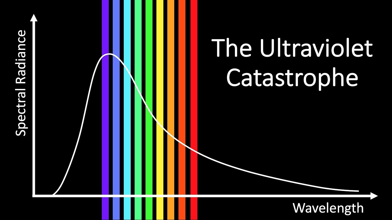
What is the Ultraviolet Catastrophe? — Physics Explained

Physics Explained

Classical physics predicted infinite radiation at high frequencies because thermodynamics treated energy as continuous, forcing Max Planck to restrict harmonic wave emissions to discrete energy packets.

AI-assisted summary of What is the Ultraviolet Catastrophe? — original source. Check the original for full context.

Source published:

Key ideas

  • Classical physics combined Maxwellian electromagnetism and Boltzmann thermodynamics to derive the Rayleigh-Jeans law, which predicted that a heated black body radiates infinite energy at short wavelengths—a failure termed the ultraviolet catastrophe. (0:00)
  • The classical failure stemmed from applying the equipartition theorem, which assigned an average energy of kT to every standing wave mode regardless of frequency. (25:15)
  • Max Planck resolved the crisis on December 14, 1900, by postulating that energy is exchanged in discrete packets (ε = hf), deriving an average oscillator energy that smoothly drops to zero at high frequencies. (33:09)
  • William Coblentz provided definitive experimental validation for Planck's radiation law in 1916, obtaining a measurement for Planck's constant h that closely aligns with modern accepted values. (37:45)

Detailed notes

## Background Published on YouTube by the educational channel Physics Explained on August 22, 2020, this video examines the ultraviolet catastrophe and Max Planck's revolutionary resolution of the theoretical crisis. Following the pedagogical structure of Eisberg and Resnick's textbook 'Quantum Physics of Atoms, Molecules, Solids, Nuclei, and Particles', the presentation walks through the classical derivations of Lord Rayleigh and Sir James Jeans before detailing Planck's quantum postulate.

## TL;DR At the turn of the 20th century, physicists attempted to explain black-body radiation by merging Maxwellian electromagnetism with classical thermodynamics, leading Lord Rayleigh and Sir James Jeans to calculate the density of standing wave modes inside a reflective cavity. Because the classical equipartition theorem assigned an average energy of kT to every harmonic mode regardless of frequency, their model predicted that total energy density diverged to infinity at short wavelengths—a theoretical failure termed the ultraviolet catastrophe. Recognizing that empirical spectra dropped to zero at high frequencies, Max Planck resolved the crisis by discarding continuous energy integration in favor of discrete energy packets proportional to frequency, ε = hf. Planck's discrete statistical derivation successfully matched empirical black-body curves across all wavelengths while reproducing the Rayleigh-Jeans limit at long wavelengths, sparking the birth of quantum mechanics.

## Atmosphere & style The presentation carries the methodical, cerebral cadence of an advanced university lecture, grounded in quiet intellectual focus and detailed mathematical transparency. Watching the video feels like working through a classic blackboard derivation, where geometric constraints, boundary conditions, and calculus proofs are built out with patient, step-by-step clarity. The measured, analytical narration imbues the narrative with a sense of historical gravitas, transforming what could be dry textbook equations into the dramatic unraveling of classical physics and a reluctant genius's desperate leap into the quantum realm.

## Bulletin - [00:00](https://www.youtube.com/watch?v=rCfPQLVzus4&t=0s) Classical physics combined Maxwellian electromagnetism and Boltzmann thermodynamics to derive the Rayleigh-Jeans law, which predicted that a heated black body radiates infinite energy at short wavelengths—a failure termed the ultraviolet catastrophe. - [25:15](https://www.youtube.com/watch?v=rCfPQLVzus4&t=1515s) The classical failure stemmed from applying the equipartition theorem, which assigned an average energy of kT to every standing wave mode regardless of frequency. - [33:09](https://www.youtube.com/watch?v=rCfPQLVzus4&t=1989s) Max Planck resolved the crisis on December 14, 1900, by postulating that energy is exchanged in discrete packets (ε = hf), deriving an average oscillator energy that smoothly drops to zero at high frequencies. - [37:45](https://www.youtube.com/watch?v=rCfPQLVzus4&t=2265s) William Coblentz provided definitive experimental validation for Planck's radiation law in 1916, obtaining a measurement for Planck's constant h that closely aligns with modern accepted values.

## Key takeaways - [00:00](https://www.youtube.com/watch?v=rCfPQLVzus4&t=0s) By the end of the 19th century, applying thermodynamics and electromagnetism to thermal radiation produced an unphysical prediction of infinite emitted energy at high frequencies, known as the ultraviolet catastrophe. - [02:08](https://www.youtube.com/watch?v=rCfPQLVzus4&t=128s) An ideal black body is a perfect absorber and emitter whose radiation intensity distribution depends solely on temperature, independent of material or geometry. - [02:08](https://www.youtube.com/watch?v=rCfPQLVzus4&t=128s) The Jeans cube uses a metallic cavity with a pinhole to trap and thermalize radiation, ensuring that the sampled emission reflects internal equilibrium radiation. - [05:14](https://www.youtube.com/watch?v=rCfPQLVzus4&t=314s) Empirical radiation laws established that total intensity scales as T⁴ (Stefan-Boltzmann law) and peak wavelength shifts inversely with temperature (Wien's displacement law). - [07:51](https://www.youtube.com/watch?v=rCfPQLVzus4&t=471s) Rayleigh and Jeans tackled the problem by calculating the electromagnetic standing-wave density of states inside a cavity and multiplying it by the average thermal energy per mode. - [13:29](https://www.youtube.com/watch?v=rCfPQLVzus4&t=809s) Electromagnetic boundary conditions on metallic cavity walls require tangential electric fields to vanish, quantizing allowed wavelengths to λ = 2L/n. - [21:40](https://www.youtube.com/watch?v=rCfPQLVzus4&t=1300s) Extending standing-wave counting to a 3D spherical octant and accounting for two orthogonal polarizations yields a density of states that scales with the square of the frequency: N(f) df = (8πL³/c³) f² df. - [25:15](https://www.youtube.com/watch?v=rCfPQLVzus4&t=1515s) Classical equipartition dictates that each standing wave acts as a simple harmonic oscillator with an average total energy of kT. - [28:12](https://www.youtube.com/watch?v=rCfPQLVzus4&t=1692s) The continuous Boltzmann distribution yields an average energy of kT because energy is assumed to be infinitely divisible from zero to infinity. - [29:54](https://www.youtube.com/watch?v=rCfPQLVzus4&t=1794s) Combining the 3D density of states with average energy kT produces the Rayleigh-Jeans law, ρ(λ) dλ = (8πkT / λ⁴) dλ, which catastrophically diverges as wavelength approaches zero. - [33:09](https://www.youtube.com/watch?v=rCfPQLVzus4&t=1989s) Planck recognized that the equipartition average energy of kT works at long wavelengths but must approach zero at high frequencies, requiring average energy to depend directly on frequency. - [35:03](https://www.youtube.com/watch?v=rCfPQLVzus4&t=2103s) By replacing continuous integration with discrete summation over energy states E = nε, Planck derived the average mode energy as ε / (e^(ε/kT) - 1). - [35:03](https://www.youtube.com/watch?v=rCfPQLVzus4&t=2103s) Setting ε = hf correctly recovers the classical limit kT at low frequencies while suppressing high-frequency emission exponentially, eliminating the ultraviolet divergence. - [37:45](https://www.youtube.com/watch?v=rCfPQLVzus4&t=2265s) Planck's resulting radiation law matched empirical blackbody spectra across the entire frequency range and provided the conceptual foundation for Bohr's quantum model of the atom. - [38:53](https://www.youtube.com/watch?v=rCfPQLVzus4&t=2333s) Planck described the introduction of energy quantization as an 'act of desperation' after six years of attempting to solve the radiation equilibrium problem within classical thermodynamics.

## Detailed walkthrough ### [00:00](https://www.youtube.com/watch?v=rCfPQLVzus4&t=0s) The Triumph of 19th-Century Physics and the Emission Dilemma

By the close of the 19th century, physics seemed to be reaching its zenith. The established principles of thermodynamics had powered the Industrial Revolution, Michael Faraday had unraveled the generation of electricity, and James Clerk Maxwell’s unification of electric and magnetic fields had uncovered that light is fundamentally an electromagnetic wave. Confident in the sweeping explanatory power of these frameworks, physicists turned their sights to remaining foundational puzzles. Among the most prominent was explaining how heated matter radiates light.

It was a matter of everyday observation that heating a piece of metal alters its glow: it transitions from a dull red to orange-red, to yellow, and ultimately to a dazzling blueish-white, growing steadily brighter along the way. Explaining how the brightness (intensity) of emitted radiation depended on wavelength (color) meant probing the fundamental mechanics of how matter interacts with light. However, applying Maxwellian electromagnetism alongside classical thermodynamics produced an absurd result: theory demanded that any hot body should radiate an infinite amount of energy at short wavelengths and high frequencies. Because this runaway emission lay in the high-frequency ultraviolet spectrum, the theoretical breakdown was coined the "ultraviolet catastrophe."

```mermaid flowchart TD accTitle: The Ultraviolet Catastrophe Failure Path accDescr: Classical theory combines Maxwell's equations and thermodynamics, predicting infinite energy at high frequencies.

subgraph Classical_Foundations ["Classical Foundations"] A["Maxwellian Electromagnetism<br/>(Light as continuous wave)"] B["Classical Thermodynamics<br/>(Equipartition theorem)"] end

subgraph The_Breakdown ["The Theoretical Crisis"] C["Combined Classical Prediction"] D["Infinite Energy at High Frequencies<br/>(Ultraviolet Catastrophe)"] end

A --> C B --> C C --> D D --> E["Planck's Energy Quantization<br/>(Discrete packets / chunks)"] ```

The narrator emphasizes that this disaster signaled the utter collapse of the classical worldview:

> “It represented a complete failure of classical physics and it was in attempting to solve this problem that Max Planck was forced to introduce the revolutionary concept of energy quantization the idea that energy is transferred discretely in chunks rather than continuously after Planck's work on this topic the world would never be the same again.”

[02:08](https://www.youtube.com/watch?v=rCfPQLVzus4&t=128s) Black Bodies, Thermal Equilibrium, and the Jeans Cube

When incident radiation strikes an object, portions of it are reflected, transmitted, or absorbed. Dark surfaces absorb significantly more incident light and reflect far less than lighter surfaces, explaining both their visual darkness and why black surfaces heat up much faster in direct sunlight. An idealized physical object that absorbs 100% of incident radiation without reflecting or transmitting any is termed a black body. A black body in an environment cooler than itself radiates energy away until thermal equilibrium is established; if placed in a warmer environment, it absorbs ambient energy until their temperatures match. Consequently, an ideal black body is both a perfect absorber and a perfect emitter of radiation.

Crucially, experimental investigations revealed that black-body emission profiles are universal: the intensity distribution across wavelengths depends solely on the temperature of the body, completely independent of its physical shape, geometry, or material makeup. To study this phenomenon under controlled conditions, physicists utilized an idealized apparatus known as the Jeans cube—named after Sir James Jeans, who, alongside Lord Rayleigh, made the first major theoretical push to explain black-body spectra.

```mermaid flowchart LR accTitle: Jeans Cube Cavity Absorption and Emission accDescr: Radiation enters through a tiny hole in a cubic metallic box, reflects until absorbed, and thermal radiation leaks out in identical profile.

subgraph Cavity_Mechanism ["Jeans Cube Mechanism"] IN["Incident Outside Radiation"] -->|"Enters pinhole"| HOLE["Small Aperture (Black Body)"] HOLE -->|"Internal bounces"| WALLS["Conducting Metallic Walls"] WALLS -->|"Absorbs & re-emits"| EQUIL["Thermal Equilibrium Radiation Inside Cavity"] EQUIL -->|"Small fraction escapes"| OUT["Emitted Black-Body Radiation"] end ```

The Jeans cube is constructed as a metallic hollow cubic box featuring a tiny pinhole on one face: - Radiation entering through the pinhole bounces repeatedly between internal conducting walls until fully absorbed, leaving almost zero probability of escaping back out; thus, the hole itself acts as an ideal absorber. - When the cavity walls are heated uniformly, they populate the enclosure with internal thermal radiation. A small fraction continually escapes through the pinhole. - Because the aperture samples the internal radiation field, the emitted beam shares the exact universal black-body intensity profile present throughout the interior of the cavity.

[05:14](https://www.youtube.com/watch?v=rCfPQLVzus4&t=314s) Empirical Radiation Laws: Lummer, Pringsheim, Stefan-Boltzmann, and Wien

Precision measurements of black-body cavity spectra carried out by Otto Lummer and Ernst Pringsheim supplied the empirical bedrock for theorists. Their experiments tracked spectral radiance—defined as the emitted intensity per unit wavelength, having physical units of watts per cubic meter ($\text{W}/\text{m}^3$)—as a function of wavelength across various temperatures. The total emitted intensity corresponds to the area under the spectral radiance curve, obtained mathematically by integrating spectral radiance over all wavelengths.

Lower temperatures yield broad, flat curves, whereas rising temperatures sharply elevate the curve area and shift its peak. From these experimental curves, two foundational empirical laws were verified:

1. **The Stefan-Boltzmann Law**: States that the total radiated intensity is directly proportional to the fourth power of absolute temperature ($I \propto T^4$). Graphically, as the temperature increases, the total area under the spectral curve expands dramatically. 2. **Wien’s Displacement Law**: Describes the shift in peak emission wavelength ($\lambda_{\text{max}}$) toward shorter wavelengths as the temperature rises ($\lambda_{\text{max}} \propto 1/T$). This matches the everyday experience of heated metal shifting its visible glow from red to orange to yellow.

Despite the elegance of these two empirical summaries, physicists remained unsatisfied. They wanted a complete mathematical function for the spectral radiance curve and demanded a first-principles derivation rooted directly in the fundamental laws of nature.

[07:51](https://www.youtube.com/watch?v=rCfPQLVzus4&t=471s) Rayleigh and Jeans' Theoretical Strategy

Lord Rayleigh and Sir James Jeans took on the challenge of deriving the black-body curve from the ground up by combining the two crowning pillars of late-19th-century physics: - **Maxwell's Electromagnetism**: Characterizing light as continuous, self-propagating electromagnetic waves traveling through a vacuum at speed $c$. - **Boltzmann's Statistical Thermodynamics**: Formulating temperature as a statistical average of the microscopic energies distributed across the constituent particles of a physical system.

Rather than calculating the outgoing spectral radiance directly, Rayleigh and Jeans streamlined their approach by first determining the spectral energy density, $u(f, T)$, inside the volume of the cavity. The spectral energy density represents the thermal radiation energy stored per unit volume at temperature $T$ within the frequency bracket between $f$ and $f + df$. Because the cavity radiation is isotropic and continually samples the pinhole, the exterior spectral radiance is proportional to this internal energy density by a geometric factor of $c / (4\pi)$.

To derive this energy density, Rayleigh and Jeans formulated a clear three-step program: 1. Determine the total number of electromagnetic standing-wave modes that can physically fit inside the boundary conditions of the cubic cavity within a frequency range. 2. Calculate the classical average energy assigned to each individual wave mode under thermal equilibrium. 3. Multiply the mode density by the average mode energy to establish the total energy density across the frequency spectrum.

[10:18](https://www.youtube.com/watch?v=rCfPQLVzus4&t=618s) Traveling Waves and the Principle of Superposition

To mathematically describe electromagnetic radiation trapped within an enclosed cavity, the radiation must first be treated as classical waves. A wave traveling to the right along the $x$-axis is represented by the sinusoidal displacement function $y(x, t) = A \sin(kx - \omega t)$. Here, $y$ specifies the displacement at position $x$ and time $t$. Because the maximum value of the sine function is 1, the prefactor $A$ defines the amplitude, representing the maximum physical displacement from equilibrium—comparable to the peak height of a vibrating rope. The minus sign governing the phase shift ensures that as time increases, the wave profile propagates toward the right.

The spatial and temporal properties of this wave are governed by two fundamental constants. The parameter $k$ is the wave number, defined explicitly as $k = \frac{2\pi}{\lambda}$ where $\lambda$ is the wavelength, signifying the spatial frequency of the oscillation. In contrast, $\omega$ represents the angular frequency, directly proportional to the temporal frequency—the count of complete wave cycles traversing a given point per second. Inverting the direction of motion requires simply changing the relative sign: a wave moving to the left is written as $y(x, t) = A \sin(kx + \omega t)$.

When two counter-propagating waves occupy the same region, they obey the principle of superposition, which dictates that the resulting spatial displacement is the arithmetic sum of the individual waveforms. Adding the right-moving and left-moving waves yields $y_{\text{net}} = A \sin(kx - \omega t) + A \sin(kx + \omega t)$. Applying the standard trigonometric identity $\sin(a - b) + \sin(a + b) = 2 \sin a \cos b$, with $a = kx$ and $b = \omega t$, collapses this sum into a single separated expression: $y_{\text{net}} = 2A \sin(kx) \cos(\omega t)$. This produces a stationary wave—or standing wave—pattern where the spatial envelope remains entirely fixed in place, oscillating solely up and down rather than traveling across space.

- As the speaker summarizes the behavior of this combined pattern: “It's called a stationary wave pattern for obvious reasons because the pattern isn't moving left or right, it's just moving up and down.”

---

[13:29](https://www.youtube.com/watch?v=rCfPQLVzus4&t=809s) Standing Waves and Boundary Conditions in the Jeans Cube

Applying this wave picture to the radiation enclosed in a Jeans cube requires establishing physical boundary conditions. Assuming a metallic cube with sides of length $L$ aligned along the $x$, $y$, and $z$ axes, any electromagnetic wave reflecting between opposite faces decomposes into directional components. Electromagnetic radiation consists of transverse vibrations whose electric field oscillates perpendicularly to the direction of propagation. For radiation propagating along the $x$-axis toward a boundary wall, the propagation vector is perpendicular to the wall, meaning the electric field lies entirely parallel to the metallic surface.

Because metal contains mobile electric charges that shift instantaneously to neutralize any tangential electric fields, a conducting wall cannot sustain a parallel electric field at its boundary. Consequently, the electric field strength $E$ must strictly vanish at the walls. Translating the standing displacement function into an electric field mode yields $E(x, t) = 2A \sin(kx) \cos(\omega t)$. At the front boundary $x = 0$, the condition $E(0, t) = 0$ is automatically satisfied since $\sin(0) = 0$. However, enforcing zero amplitude at the opposing boundary $x = L$ requires that $\sin(kL) = 0$.

```mermaid flowchart TD accTitle: Standing Wave Boundary Condition Flow accDescr: Flowchart illustrating how metallic boundary conditions restrict allowed wavelengths and frequencies in a cavity. subgraph Boundary ["Boundary Constraints"] A["Metallic Cube Wall at x = L"] --> B["Tangential E-field vanishes: E(L) = 0"] B --> C["sin(kL) = 0"] end subgraph Quantization ["Mode Quantization"] C --> D["kL = n * pi"] D --> E["k = n * pi / L"] E --> F["Wavelength: lambda = 2L / n"] F --> G["Frequency: f = n * c / (2L)"] end ```

The sine function equals zero only when its argument is an integer multiple of $\pi$ radians, leading directly to $kL = n\pi$, or $k = \frac{n\pi}{L}$ for integers $n = 1, 2, 3, \dots$. Substituting $k = \frac{2\pi}{\lambda}$ reveals that the permitted wavelengths inside the cube are strictly quantized: $\lambda = \frac{2L}{n}$. When $n = 1$, the longest allowed wavelength is $\lambda = 2L$; when $n = 2$, $\lambda = L$; when $n = 3$, $\lambda = \frac{2L}{3}$, and so forth. Only discrete standing wave modes with nodes located at both boundaries can exist within the cavity walls.

- “Therefore the electric field must be zero at the walls of the container that is the stationary wave associated with the x component of the radiation must have a node aka zero amplitude at x equals zero and x equals l.” - Allowed wavelengths: $\lambda_n = \frac{2L}{n}$, where $n \in \{1, 2, 3, 4, 5, 6, \dots\}$. - Allowed frequencies: $f_n = \frac{c}{\lambda_n} = \frac{n c}{2L}$.

---

[18:00](https://www.youtube.com/watch?v=rCfPQLVzus4&t=1080s) Density of States in One Dimension

To count the total number of standing modes allowed within any given frequency interval, the discrete integer values of $n$ can be mapped onto a linear state diagram. Rearranging the frequency relation $f = \frac{n c}{2L}$ gives the mode index as a linear function of frequency: $n = \frac{2L}{c} f$. Defining the distance from the origin on this axis as $d = \frac{2L}{c} f$, every integer increment of $n$ corresponds to one allowed standing wave state.

To determine the number of allowed states $N(f) df$ within an incremental frequency range from $f$ to $f + df$, one computes the difference in distance along the axis between the two frequency limits: $$N(f) df = \frac{2L}{c}(f + df) - \frac{2L}{c}f = \frac{2L}{c} df$$ Because the mode points are uniformly distributed along the $n$-axis, the number of available modes in one dimension depends strictly on the bandwidth $df$ and is entirely independent of the center frequency $f$.

This preliminary density of states must be corrected to account for physical wave properties. Because electromagnetic waves are transverse, every spatial mode can support two independent, orthogonal polarization states. Multiplying by this polarization factor of 2 yields the complete one-dimensional density of states: $$N(f) df = \frac{4L}{c} df$$

- “Since the points are distributed uniformly along the n axis it is apparent that the number of points falling between the two limits will be proportional to df but will not actually depend on f.” - Polarization factor: 2 independent states per frequency mode. - Final 1D mode count: $N(f) df = \frac{4L}{c} df$.

---

[19:30](https://www.youtube.com/watch?v=rCfPQLVzus4&t=1170s) Generalizing Standing Waves to Two and Three Dimensions

Extending this counting technique to the realistic three-dimensional Jeans cube begins with a two-dimensional case across the $x$ and $y$ planes. Radiation with wavelength $\lambda$ propagating in an arbitrary direction can be defined by the direction angles $\alpha$ and $\beta$ measured relative to the $x$ and $y$ axes. Because both directional components independently reflect between opposing walls to set up standing waves, the oblique wave itself forms a stationary wave pattern throughout the interior.

The nodes of this oblique standing wave appear as a sequence of parallel planes perpendicular to the propagation vector, spaced by half a wavelength ($\frac{\lambda}{2}$). The projections of this wave onto the respective coordinate axes create effective component wavelengths $\lambda_x$ and $\lambda_y$. Through basic right-triangle trigonometry on the geometry of the nodal planes: $$\frac{\lambda}{2} = \frac{\lambda_x}{2} \cos\alpha \implies \lambda = \lambda_x \cos\alpha \implies \lambda_x = \frac{\lambda}{\cos\alpha}$$ $$\frac{\lambda}{2} = \frac{\lambda_y}{2} \cos\beta \implies \lambda = \lambda_y \cos\beta \implies \lambda_y = \frac{\lambda}{\cos\beta}$$

Connecting these projected wavelengths to the cavity dimensions requires enforcing the box boundary conditions along each axis: $\lambda_x = \frac{2L}{n_x}$ and $\lambda_y = \frac{2L}{n_y}$. Equating these relations reveals the mode integers in terms of the direction cosines: $$n_x = \frac{2L \cos\alpha}{\lambda}, \quad n_y = \frac{2L \cos\beta}{\lambda}$$ This formulation extends directly to three dimensions by introducing the angle $\gamma$ relative to the $z$-axis, yielding $\lambda_z = \frac{2L}{n_z}$ and $n_z = \frac{2L \cos\gamma}{\lambda}$. Summing the squares of all three mode numbers establishes a single governing relation: $$n_x^2 + n_y^2 + n_z^2 = \left(\frac{2L}{\lambda}\right)^2 \left(\cos^2\alpha + \cos^2\beta + \cos^2\gamma\right)$$

- “The radiation in this arbitrary direction must form a stationary wave since we've already seen that the x and y components form stationary waves.” - Direction cosine relation in 2D: $\lambda_x = \frac{\lambda}{\cos\alpha}$, $\lambda_y = \frac{\lambda}{\cos\beta}$. - 3D mode relations: $n_x = \frac{2L \cos\alpha}{\lambda}$, $n_y = \frac{2L \cos\beta}{\lambda}$, $n_z = \frac{2L \cos\gamma}{\lambda}$.

[21:40](https://www.youtube.com/watch?v=rCfPQLVzus4&t=1300s) Deriving the 3D Density of States in Frequency Space

The derivation begins by recalling the three-dimensional directional cosine relation, which is the 3D geometric extension of Pythagoras' theorem:

$$\cos^2\alpha + \cos^2\beta + \cos^2\gamma = 1$$

Applying this to standing waves inside a cubic cavity of side length $L$ yields:

$$n_x^2 + n_y^2 + n_z^2 = \left(\frac{2L}{\lambda}\right)^2$$

Rearranging for the wavelength gives:

$$\lambda = \frac{2L}{\sqrt{n_x^2 + n_y^2 + n_z^2}}$$

Converting this relation into frequency via $f = c / \lambda$ results in:

$$f = \frac{c}{2L}\sqrt{n_x^2 + n_y^2 + n_z^2}$$

To calculate the density of states within a frequency band, the system is mapped onto a coordinate space defined by integer grid axes labeled by $(n_x, n_y, n_z)$. Standing wave states are represented as points in this grid. Geometrically, states with a total radius $r = \sqrt{n_x^2 + n_y^2 + n_z^2}$ correspond to a sphere centered at the origin. Because physical wave modes require positive integers for $(n_x, n_y, n_z)$, the physical domain occupies only the positive octant—exactly one-eighth ($\frac{1}{8}$) of the total sphere's volume.

```mermaid flowchart TD accTitle: Counting 3D Cavity Wave Modes accDescr: Pipeline showing geometric transformation from discrete mode numbers into a continuous frequency density of states. subgraph Geometry["Spherical Octant Geometry"] A["Radius: r = √(nx² + ny² + nz²)"] --> B["Relate to frequency: r = 2Lf / c"] B --> C["Segment volume: (1/8) × 4πr² dr = (π/2) r² dr"] end subgraph FrequencyConversion["Frequency Substitution"] C --> D["Substitute r and dr in terms of f and df"] D --> E["Single polarization count: N(f) df = (4πL³ / c³) f² df"] end subgraph TotalDensity["Final Density of States"] E --> F["Multiply by 2 for EM polarizations"] F --> G["Total states: N(f) df = (8πL³ / c³) f² df"] end ```

Expressing the radius $r$ in terms of frequency yields $r = \frac{2Lf}{c}$, which when differentiated gives $\frac{dr}{df} = \frac{2L}{c}$, or $dr = \frac{2L}{c}\,df$. The number of mode states $N(r)\,dr$ contained within a spherical shell segment between radius $r$ and $r + dr$ is the volume of the shell restricted to that positive octant:

$$N(r)\,dr = \frac{1}{8} (4\pi r^2\,dr) = \frac{\pi r^2\,dr}{2}$$

Substituting $r = \frac{2Lf}{c}$ and $dr = \frac{2L}{c}\,df$ into this geometric shell volume gives:

$$N(f)\,df = \frac{\pi}{2} \left(\frac{2L}{c}\right)^3 f^2\,df = \frac{4\pi L^3}{c^3} f^2\,df$$

Because electromagnetic radiation contains two independent orthogonal transverse polarization states for each mode, this expression must be multiplied by a factor of 2. The total number of states in the frequency interval $df$ becomes:

$$N(f)\,df = \frac{8\pi L^3}{c^3} f^2\,df$$

The speaker emphasizes the physical consequence of this algebraic scaling: “Notice that the number scales with $f$ squared, indicating that the number of states grows rapidly at high frequency or short wavelength.”

- Directional cosine relation: $\cos^2\alpha + \cos^2\beta + \cos^2\gamma = 1$ - Mode index radius relation: $r = \sqrt{n_x^2 + n_y^2 + n_z^2} = \frac{2Lf}{c}$ - Shell differential: $dr = \frac{2L}{c}\,df$ - Octant geometry factor: $\frac{1}{8}$ of full spherical volume $4\pi r^2\,dr$ - Electromagnetic polarization multiplier: factor of $2$

---

[25:15](https://www.youtube.com/watch?v=rCfPQLVzus4&t=1515s) Classical Equipartition and the Average Energy per Mode

Having established the count of allowed modes inside the cavity, the analysis turns to determining the average energy carried by each individual wave. Lord Rayleigh and Sir James Jeans drew on classical thermodynamics, specifically invoking the equipartition theorem. In a classical gas in thermal equilibrium consisting of vast numbers of randomly moving particles, thermal energy is shared equally among every available degree of freedom.

In a monatomic gas, each individual atom can be visualized as a tiny rigid sphere bouncing randomly within a container. Its kinetic motion is resolved into three translational modes along the $x$, $y$, and $z$ axes. Because of the vast statistical ensemble of atoms, the kinetic energy distributes symmetrically: if $x$ joules are added to the box, precisely $\frac{x}{3}$ joules partition into kinetic energy along each coordinate axis. In thermal equilibrium, every individual degree of freedom possesses an average energy equal to:

$$\langle E \rangle = \frac{1}{2}kT$$

The speaker points out an intuitive way to understand the physical role of Boltzmann's constant $k$: “You can think of Boltzmann's constant as representing the exchange rate between the currencies of energy and temperature.” For a monatomic gas having 3 translational degrees of freedom, the average energy per particle is $3 \times \frac{1}{2}kT = \frac{3}{2}kT$, giving a total energy of $N \times \frac{3}{2}kT$ for $N$ particles.

Rayleigh and Jeans extended this logic directly to the electromagnetic standing waves in the cavity. Classical physics asserted that the equipartition theorem should govern any classical system in thermal equilibrium containing a large number of identical entities. For the cavity, these entities are standing waves, each possessing a single degree of freedom defined by its electric field amplitude. While the average kinetic energy of each wave is $\frac{1}{2}kT$, each standing wave is a simple harmonic oscillator oscillating sinusoidally in time. Because the time-averaged potential energy equals the time-averaged kinetic energy in a simple harmonic oscillator, the total average energy per standing wave is twice its kinetic energy:

$$\langle E \rangle = 2 \times \left(\frac{1}{2}kT\right) = kT$$

- Equipartition theorem origin: Classical statistical mechanics for ensembles in thermal equilibrium - Energy per quadratic degree of freedom: $\frac{1}{2}kT$ - Translational kinetic degrees of freedom for a monatomic gas: 3 (yielding $\frac{3}{2}kT$) - Cavity standing waves: 1 harmonic degree of freedom per mode - Standing wave total energy: Kinetic plus potential energy equals $kT$

---

[28:12](https://www.youtube.com/watch?v=rCfPQLVzus4&t=1692s) The Boltzmann Distribution and the Origin of $kT$

To understand where the ultraviolet catastrophe fundamentally originates, the speaker isolates the statistical mechanical foundation that produces the $\langle E \rangle = kT$ result: the continuous Boltzmann distribution. The Boltzmann distribution provides the probability density of finding a subsystem with continuous energy $E$ at temperature $T$, allowing the calculation of the ensemble average energy:

$$\langle E \rangle = \frac{\int_0^\infty E\,e^{-E / kT}\,dE}{\int_0^\infty e^{-E / kT}\,dE}$$

The speaker unpacks the physical intuition behind this quotient: “The integrand in the numerator can be thought of as the energy weighted by the probability that the entity will be found with this energy.” Integrating over all possible values yields the total weighted energy, while the denominator represents the total normalization probability across all energy states.

The evaluation of both integrals proceeds via elementary calculus: 1. **Denominator Integral**: Direct integration of the decaying exponential: $$\int_0^\infty e^{-E / kT}\,dE = \left[ -kT\,e^{-E / kT} \right]_0^\infty = 0 - (-kT) = kT$$ 2. **Numerator Integral**: Solved via integration by parts using the product rule identity $\frac{d}{dE}\left(E e^{-E/kT}\right) = e^{-E/kT} - \frac{E}{kT}e^{-E/kT}$: $$\int_0^\infty E\,e^{-E / kT}\,dE = (kT)^2$$

Taking the ratio of the two results confirms the equipartition expectation:

$$\langle E \rangle = \frac{(kT)^2}{kT} = kT$$

This classical derivation relies entirely on the continuous integration over all energy values from zero to infinity, an assumption that proves to be the ultimate point of failure in classical physics.

- Normalization integral (denominator): $\int_0^\infty e^{-E / kT}\,dE = kT$ - Expectation integral (numerator): $\int_0^\infty E\,e^{-E / kT}\,dE = (kT)^2$ - Classical average oscillator energy: $\frac{(kT)^2}{kT} = kT$

---

[29:54](https://www.youtube.com/watch?v=rCfPQLVzus4&t=1794s) Combining Results: The Rayleigh-Jeans Law in Frequency and Wavelength

With both the mode counting density and the average energy per mode established, the full energy density inside the cavity can be assembled. Energy density, denoted $\rho(f)\,df$, is defined as the total electromagnetic energy per unit volume within the frequency interval $df$. Multiplying the density of states $N(f)\,df$ by the average energy per state $\langle E \rangle = kT$, and dividing by the cavity volume $V = L^3$, gives:

$$\rho(f)\,df = \frac{N(f)\,df \times \langle E \rangle}{L^3} = \frac{\left(\frac{8\pi L^3}{c^3} f^2\,df\right) \times kT}{L^3} = \frac{8\pi f^2 kT}{c^3}\,df$$

To express the energy distribution in terms of wavelength $\lambda$ rather than frequency $f$, energy conservation across the equivalent spectral intervals requires matching energy densities:

$$\rho(\lambda)\,d\lambda = -\rho(f)\,df$$

The negative sign is physically essential: because frequency and wavelength are inversely related via $f = \frac{c}{\lambda}$, an increase in frequency corresponds to a decrease in wavelength. Differentiating $f$ with respect to $\lambda$:

$$\frac{df}{d\lambda} = -\frac{c}{\lambda^2} \implies df = -\frac{c}{\lambda^2}\,d\lambda$$

Substituting this differential and $f = \frac{c}{\lambda}$ into the energy density relation gives:

$$\rho(\lambda)\,d\lambda = \frac{8\pi \left(\frac{c}{\lambda}\right)^2 kT}{c^3} \left(\frac{c}{\lambda^2}\,d\lambda\right) = \frac{8\pi kT}{\lambda^4}\,d\lambda$$

This expression is the classical Rayleigh-Jeans law. The speaker concludes the derivation by posing the critical question about its functional behavior: “Rho of lambda $d\lambda$ equals $8\pi kT$ over lambda to the 4 $d\lambda$, and this represents the energy density in terms of the wavelength. So what does this function look like?” The sharp $\lambda^{-4}$ dependence sets up the inevitable mathematical divergence known as the ultraviolet catastrophe.

- Total spectral energy density in frequency space: $\rho(f)\,df = \frac{8\pi f^2 kT}{c^3}\,df$ - Frequency-wavelength derivative: $\frac{df}{d\lambda} = -\frac{c}{\lambda^2}$ - Final Rayleigh-Jeans law in wavelength: $\rho(\lambda)\,d\lambda = \frac{8\pi kT}{\lambda^4}\,d\lambda$ - Functional consequence: Diverges toward infinity as wavelength approaches zero ($\lambda \to 0$)

[32:02](https://www.youtube.com/watch?v=rCfPQLVzus4&t=1922s) The Ultraviolet Catastrophe and Rayleigh–Jeans Breakdown

When the spectral energy density is plotted on the $y$-axis against the wavelength on the $x$-axis, experimental measurements produce a smooth, peaked curve that rises and then rolls over toward zero at short wavelengths. However, when Lord Rayleigh and Sir James Jeans plotted their theoretical energy density function derived strictly from classical electrodynamics and thermodynamics, they arrived at an alarming divergence. At small wavelengths, their predicted energy density shoots up rapidly toward infinity.

```mermaid flowchart TD accTitle: The Ultraviolet Catastrophe Divergence accDescr: Flowchart illustrating how classical mechanics predicts infinite energy density at short wavelengths. subgraph ClassicalTheory["Classical Rayleigh-Jeans Model"] A["Equipartition of Energy: Average Energy = kT"] --> B["Density of States proportional to 1 / lambda^4"] B --> C["Energy Density proportional to kT / lambda^4"] end subgraph Divergence["The Catastrophe"] C --> D["Short Wavelengths: lambda approaches 0"] D --> E["High Frequencies: f approaches infinity"] E --> F["Energy Density tends to infinity (Ultraviolet Catastrophe)"] end ```

The mathematical reason for this divergence is embedded directly in the Rayleigh–Jeans formula. Because the energy density function is proportional to $\lambda^{-4}$, shrinking the wavelength $\lambda$ causes the denominator $\lambda^4$ to become vanishingly tiny, forcing the resulting energy density to become colossal. Framed in terms of frequency, small wavelengths correspond to high frequencies; since there is no upper frequency boundary inside an enclosed cavity or radiator, as frequency approaches infinity, the energy density likewise tends to infinity. This catastrophic breakdown of classical theory at short wavelengths earned the name the "ultraviolet catastrophe." The narrator notes the gravity of this theoretical failure:

> “Rayleigh and Jeans had demonstrated that the best understood classical laws of physics were incapable of describing even the most commonplace phenomena, namely the radiation properties of hot objects.”

- Experiments reveal a smooth distribution that drops to zero at both extremely short and extremely long wavelengths. - Classical theory yields an energy density proportional to $\lambda^{-4}$, predicting an explosive blowup in the ultraviolet and beyond.

---

[33:09](https://www.youtube.com/watch?v=rCfPQLVzus4&t=1989s) Max Planck and the Quantum Hypothesis

Out of the wreckage of classical physics emerged a revolutionary new theoretical framework. Max Planck, an unassuming German physicist who had dedicated the majority of his career to thermodynamics, tackled the blackbody radiation problem after wrestling with it for years and frequently despairing at the mathematical roadblocks. On December 14, 1900, Planck presented a landmark lecture announcing that the Rayleigh–Jeans breakdown could be eliminated, and the ultraviolet catastrophe averted, if one assumed that energy is exchanged only in discrete packets called *quanta*.

Planck began by comparing the Rayleigh–Jeans curve with the empirical data. While the Rayleigh–Jeans prediction fails catastrophically at short wavelengths, it matches real experimental measurements remarkably well at long wavelengths. This suggested that the classical equipartition theorem—which assigns an average energy of $kT$ to every standing wave mode—remains valid in the long-wavelength limit. Conversely, experimental data proved that the average energy must drop toward zero at very short wavelengths (high frequencies). Planck realized that the average energy of a standing wave cannot be a universal constant ($kT$); it must depend directly on frequency, meaning the equipartition theorem had to be abandoned.

To implement the required high-frequency cutoff, Planck modified Ludwig Boltzmann’s statistical distribution calculation. Instead of treating energy as a continuous variable where any arbitrary value is permitted, he treated it as a discrete quantity. He postulated that the total energy of an oscillator can only assume integral multiples of a basic discrete energy packet $\varepsilon$. Mathematically, this transition from continuous to discrete states required replacing the continuous integrals of classical statistical mechanics with discrete summations.

- Planck announced his quantum hypothesis to the German Physical Society on December 14, 1900. - Long-wavelength radiation empirically confirms an average energy of $\bar{\mathcal{E}} \approx kT$. - Short-wavelength radiation requires the average energy to approach zero ($\bar{\mathcal{E}} \to 0$), demanding an explicit frequency dependence. - Energy is restricted to discrete multiples: $E = n\varepsilon$, where $n = 0, 1, 2, 3, \dots$.

---

[35:03](https://www.youtube.com/watch?v=rCfPQLVzus4&t=2103s) Deriving the Quantized Average Energy

Switching to discrete energy packets fundamentally changes the average energy calculated via the Boltzmann distribution. The continuous integrals over energy are replaced with sums over state index $n$:

$$\bar{\mathcal{E}} = \frac{\sum_{n=0}^{\infty} n\varepsilon e^{-n\varepsilon / kT}}{\sum_{n=0}^{\infty} e^{-n\varepsilon / kT}}$$

Evaluating this expression involves two steps. The denominator is a standard infinite geometric series with ratio $e^{-\varepsilon / kT}$, which evaluates neatly to:

$$\sum_{n=0}^{\infty} \left(e^{-\varepsilon / kT}\right)^n = \frac{1}{1 - e^{-\varepsilon / kT}}$$

The numerator requires a calculus trick. Defining $f(\varepsilon)$ as the denominator sum, the numerator can be rewritten in differential form as $-kT \frac{df}{d(1/kT)}$ or by differentiating with respect to $\varepsilon$. Computing the derivative yields what the speaker jokingly calls a “rather ghastly expression,” but combining the numerator and denominator simplifies the entire average energy down to:

$$\bar{\mathcal{E}} = \frac{\varepsilon}{e^{\varepsilon / kT} - 1}$$

Analyzing the asymptotic limits of this equation confirms Planck’s intuition: 1. **Limit of small $\varepsilon$ ($\varepsilon \ll kT$):** The exponential $e^{\varepsilon / kT}$ can be expanded as a Taylor series, $e^{\varepsilon / kT} \approx 1 + \frac{\varepsilon}{kT} + \dots$. Substituting this into the denominator gives $(1 + \varepsilon / kT - 1) = \varepsilon / kT$. The $\varepsilon$ terms cancel out, leaving $\bar{\mathcal{E}} = kT$, exactly reproducing the classical equipartition result. 2. **Limit of large $\varepsilon$ ($\varepsilon \gg kT$):** The exponential in the denominator grows exponentially faster than the linear $\varepsilon$ in the numerator, driving the average energy $\bar{\mathcal{E}}$ smoothly to zero.

Because experimental data shows $\bar{\mathcal{E}} \to kT$ as frequency $f \to 0$, and $\bar{\mathcal{E}} \to 0$ as $f \to \infty$, Planck concluded that the energy packet $\varepsilon$ must be a strictly increasing function of frequency. Numerical curve-fitting led him to hypothesize a direct linear proportionality, introducing a new fundamental constant of nature, $h$:

$$\varepsilon = hf$$

Substituting this relation gives the final Planck formula for average energy:

$$\bar{\mathcal{E}} = \frac{hf}{e^{hf / kT} - 1}$$

---

[37:45](https://www.youtube.com/watch?v=rCfPQLVzus4&t=2265s) Planck’s Radiation Law and Experimental Confirmation

Equipped with this frequency-dependent average energy, Planck multiplied it by the classical density of states function inside a cavity to obtain the complete energy density distribution. Written as a function of wavelength $\lambda$, Planck's radiation law takes the form:

$$\rho(\lambda) \, d\lambda = \frac{8\pi hc}{\lambda^5 \left(e^{hc / \lambda kT} - 1\right)} \, d\lambda$$

When plotted, Planck's formula matches the experimental blackbody radiation curves across all wavelengths without diverging. At very long wavelengths, applying a Taylor series expansion to the exponential denominator reduces the equation directly back to the classical Rayleigh–Jeans formula, preserving the successes of classical physics where they were valid while cutting off the catastrophic high-frequency tail.

Definitive empirical validation followed. In 1916, American physicist William Coblentz performed precise, detailed experimental measurements on thermal radiation. Plotting Planck's theoretical curve as a solid line alongside experimental data points represented as circles showed remarkable, near-perfect agreement across the entire spectrum. Using his blackbody data, Coblentz determined an experimental value for Planck’s constant $h$ that sits remarkably close to the modern accepted value.

- The density of states combined with the quantized average energy resolves the ultraviolet catastrophe at all wavelengths. - A Taylor series expansion shows that Planck’s distribution naturally simplifies to the Rayleigh–Jeans distribution as $\lambda \to \infty$. - William Coblentz's 1916 experiments provided conclusive empirical proof for Planck's law and an accurate measurement of $h$.

---

[38:53](https://www.youtube.com/watch?v=rCfPQLVzus4&t=2333s) The Birth of Quantum Mechanics and Planck's "Act of Desperation"

Although Planck’s derivation originated as a targeted thermodynamic solution to blackbody cavity radiation, the quantum hypothesis triggered the birth of modern quantum mechanics. The core physical revelation was that any physical system undergoing simple harmonic motion cannot exchange energy continuously; its energy must satisfy the quantization condition:

$$E = n h f$$

In classical mechanics, an oscillator vibrating sinusoidally at frequency $f$ can take on a continuous spectrum of energy states. In Planck's formulation, energy is discrete, restricted to a ladder of allowed states where $n$ is an integer quantum number. Thirteen years after Planck’s breakthrough, in 1913, Niels Bohr adapted this energy quantization principle to construct his orbital model of the hydrogen atom, firmly establishing the quantum revolution.

Despite the monumental legacy of his discovery, Planck did not set out to overthrow physics. In a reflective quote from his later years, he candidly characterized his radical mathematical invention as a last resort:

> “Briefly summarized what I did can be described as simply an act of desperation. By nature I am peacefully inclined and reject all doubtful adventures, but by then I had been wrestling unsuccessfully for six years with the problem of equilibrium between radiation and matter, and I knew that this problem was of fundamental importance to physics. A theoretical interpretation therefore had to be found at any cost no matter how high.”

- Classical systems possess continuous energy distributions; quantum systems feature discrete energy levels indexed by quantum number $n$. - Niels Bohr leveraged Planck's discrete energy hypothesis in 1913 to create his quantum model of the atom. - Planck considered the quantum postulate an "act of desperation" after six grueling years of unsuccessful work within classical thermodynamics.

## Notable quotes > [25:15](https://www.youtube.com/watch?v=rCfPQLVzus4&t=1515s) You can think of Boltzmann's constant as representing the exchange rate between the currencies of energy and temperature. — Physics Explained

> [32:02](https://www.youtube.com/watch?v=rCfPQLVzus4&t=1922s) Rayleigh and Jeans had demonstrated that the best understood classical laws of physics were incapable of describing even the most commonplace phenomena, namely the radiation properties of hot objects. — Physics Explained

## Mentioned Michael Faraday, James Clerk Maxwell, Max Planck, Sir James Jeans, Lord Rayleigh, Otto Lummer, Ernst Pringsheim, Ludwig Boltzmann, William Coblentz, Niels Bohr, Quantum physics of atoms, molecules, solids, nuclei and particles, Robert Eisberg, Robert Resnick, The Quantum Story, Jim Baggot, Quantum Physics for Dummies, Steven Holzner, Thirty Years that Shook Physics, George Gamow, Inward Bound, Abraham Pais, German Physical Society

## Video description This video provides a detailed explanation of the ultraviolet catastrophe and Max Planck's solution to the problem following the presentation of Esiberg and Resnick in their textbook 'Quantum physics of atoms, molecules, solids, nuclei and particles'. The work of Rayleigh and Jeans is discussed in detail, as well as the quantum hypothesis proposed by Planck.

References for this video:

Quantum physics of atoms, molecules, solids, nuclei and particles - Eisberg and Resnick The Quantum Story - Jim Baggot Quantum Physics for Dummies - Steven Holzner Thirty Years that Shook Physics - Gamow Inward Bound - Abraham Pais

You can help support this channel via the Physics Explained Patreon account: https://www.patreon.com/physicsexplained

You can follow me on instagram: https://www.instagram.com/physics_explained_ig

You can follow me on Twitter: https://twitter.com/PhysicsExplain1

[Source](https://www.youtube.com/watch?v=rCfPQLVzus4)

中文简报

普朗克引入能量量子化以消除经典黑体发散 由于经典热力学将能量视为连续的,经典物理学预测高频辐射会趋于无限大,这迫使马克斯·普朗克将谐波辐射限制为离散的能量包。 20世纪初,物理学家试图结合麦克斯韦电磁学与经典热力学来解释黑体辐射,瑞利勋爵和詹姆斯·金斯爵士据此计算了反射腔内的驻波模式密度。由于经典能量均分定理无论频率高低都赋予每个谐波模式kT的平均能量,他们的模型预测总能量密度在短波长处发散至无穷大——这一理论崩溃被称为“紫外灾难”。马克斯·普朗克认识到实验光谱在高频处会降至零,通过舍弃连续能量积分,转而引入与频率成正比的离散能量包(ε = hf)解决了这一危机。普朗克的离散统计推导成功拟合了所有波长的黑体实验曲线,并在长波极限下还原了瑞利-金斯定律,由此开启了量子力学的诞生。 经典物理学结合麦克斯韦电磁学与玻尔兹曼热力学导出了瑞利-金斯定律,该定律预测受热黑体在短波长处辐射出无限能量——这一理论失败被称为“紫外灾难”。 (0:00) 经典理论的失败根源于能量均分定理的应用,该定理不考虑频率差异,赋予每个驻波模式kT的平均能量。 (25:15) 1900年12月14日,马克斯·普朗克提出能量以离散能量包(ε = hf)的形式进行交换,从而化解了危机,推导出的振子平均能量在高频下平滑趋近于零。 (33:09) 威廉·科布伦茨于1916年为普朗克辐射定律提供了决定性的实验验证,其测得的普朗克常数h与现代公认值高度吻合。 (37:45)

Reading summary

Physics Explained details how classical physics failed to explain black-body radiation, predicting an impossible infinite energy emission at short wavelengths known as the ultraviolet catastrophe. The breakdown was resolved when Max Planck introduced energy quantization, replacing classical continuous radiation models and establishing the foundation for quantum mechanics. Cavity Boundary Conditions and State Density (21:40) To model black-body radiation independently of material shape or composition, theorists evaluated thermal radiation within a reflective metallic enclosure known as the Jeans cube. Because mobile electric charges in conducting walls neutralize tangential electric fields, electromagnetic standing waves require nodes where the electric field strictly vanishes at the boundaries. This condition constrains allowed wavelengths along each axis to λ = 2L / n, establishing discrete resonant frequencies fn = n c / (2L). Extending these constraints to three dimensions using directional cosines maps wave modes onto an integer grid (nx, ny, nz) within the positive octant of a sphere of radius r = 2Lf / c. Evaluating the differential volume of this spherical shell and accounting for two independent transverse polarization states yields the 3D density of states: N(f) df = (8π L³ / c³) f² df. This geometric result demonstrates that the number of permissible standing-wave states inside the cavity grows quadratically with frequency. Classical Equipartition and the Rayleigh-Jeans Breakdown (25:15) To determine cavity energy density, classical thermodynamics applied the equipartition theorem, which dictates that thermal energy distributes equally among all active degrees of freedom in thermal equilibrium. Because each standing wave mode behaves as a simple harmonic oscillator with equal average kinetic and potential energy (½kT each), classical theory assigned each mode an average energy of <E> = kT. Evaluating continuous Boltzmann probability integrals appeared to rigorously justify this mode energy. Multiplying the mode density by <E> = kT and converting from frequency to wavelength produced the Rayleigh-Jeans law: ρ(λ) dλ = (8π kT / λ⁴) dλ. While this formula matched empirical data at long wavelengths, its inverse fourth-power dependence on wavelength meant that as λ approached zero, the predicted energy density diverged toward infinity. Termed the ultraviolet catastrophe, this unphysical prediction revealed that combining Maxwellian electrodynamics with classical equipartition completely failed to describe thermal emission. Energy Quantization and Planck's Distribution Law (35:03) Max Planck eliminated the runaway high-frequency divergence by abandoning the assumption that oscillators absorb and emit energy continuously. Postulating that energy is exchanged only in discrete integer packets (E = nε), Planck replaced classical continuous integrals with discrete summations over energy states. This revised statistical mechanics produced a modified average energy per mode, E-bar = ε / (e^(ε / kT) - 1), which approaches kT when ε is small but drops toward zero when ε is large. To ensure that high-frequency modes were suppressed while low-frequency modes retained classical behavior, Planck set the energy packet directly proportional to frequency: ε = hf, introducing the fundamental constant h. Combining this frequency-dependent average energy with the classical density of states produced Planck's radiation law: ρ(λ) dλ = [8π hc / (λ⁵ (e^(hc / λkT) - 1))] dλ. Through Taylor series expansion, this expression reduces to the Rayleigh-Jeans law at long wavelengths while eliminating the short-wavelength divergence. Empirical Verification and Broader Quantum Implications (37:45) Precision experiments firmly corroborated Planck's theoretical formula. In 1916, American physicist William Coblentz conducted thermal radiation measurements that demonstrated near-perfect agreement with Planck's curve across all wavelengths and yielded an empirical estimate for Planck's constant h close to modern values. This confirmed that Planck's law successfully integrated the earlier empirical findings of the Stefan-Boltzmann law and Wien's displacement law. Although Planck later described his discrete mathematical postulate as an "act of desperation" after six years of failed attempts within classical thermodynamics, the assumption that oscillators operate on quantized ladders (E = n h f) transformed modern physics. Thirteen years later, in 1913, Niels Bohr adapted Planck's energy quantization principle to formulate his quantum model of the hydrogen atom, permanently departing from classical continuity. While Planck's formulation resolved the black-body paradox by introducing energy quanta as an emergency mathematical remedy, it simultaneously exposed the fundamental limits of classical continuous field theories, initiating the development of modern quantum mechanics.

精炼阅读摘要

节目指出,19世纪末经典电磁学与热力学的结合在解释黑体辐射时得出了高频能量发散的荒谬结论,即“紫外灾难”;马克斯·普朗克通过打破经典连续性假定、提出离散的能量量子化假设,成功消除了发散并奠定了量子力学的基础。 黑体辐射的实验规律与经典理论设想 (2:08) 在日常生活中,加热金属时其发光颜色会随温度升高从暗红、橙红、黄色转变为蓝白色,且亮度持续增加。物理学将能够百分之百吸收外来辐射且不发生反射或透射的理想物体定义为黑体,在达到热平衡时它同样是最理想的辐射体。奥托·卢默(Otto Lummer)与恩斯特·普林斯海姆(Ernst Pringsheim)等人的精确测量证实,黑体辐射的光谱辐射度分布与物体的几何形状或材料构成无关,仅取决于绝对温度。这一实验基础确立了两个关键经验定律:总辐射强度与温度四次方成正比的斯忒藩-玻尔兹曼定律(Stefan-Boltzmann Law),以及峰值波长与温度成反比的维恩位移定律(Wien's Displacement Law)。 瑞利-金斯定律的推导与紫外灾难的爆发 (7:51) 为了从第一性原理推导黑体光谱,瑞利勋爵(Lord Rayleigh)与詹姆斯·金斯爵士(Sir James Jeans)结合麦克斯韦电磁学和玻尔兹曼统计热力学,以金属空腔(Jeans cube)为模型展开推导。由于空腔导电金属壁在边界处的切向电场必须为零,腔内电磁驻波的波长和频率被离散化。经三维空间计算并计入电磁波的两种正交偏振态,腔内单位频率间隔的状态数正比于频率平方,即 N(f)df = (8πL³/c³)f²df。随后,他们利用经典能量均分定理,将每个驻波模式视为简谐振子,认为其在热平衡下的平均能量恒为 kT(基于连续玻尔兹曼分布积分得出)。二者相乘并除以体积后,得到的波长能量密度分布为 ρ(λ)dλ = (8πkT/λ⁴)dλ。当波长趋于零(频率趋于无穷大)时,分母中的 λ⁴ 导致辐射能量密度爆炸式趋于无穷大,即所谓的“紫外灾难”,暴露出经典物理在解释微观辐射问题时的彻底崩溃。 普朗克的能量量子化假设与均分定理的废除 (33:09) 瑞利-金斯定律在长波区域与实测数据高度吻合,而在短波区域严重失效。这一对比促使马克斯·普朗克意识到,经典均分定理中驻波模式平均能量恒为 kT 的假设在高频端并不成立,振子的平均能量必须依赖于频率,并在高频端趋近于零。1900年12月14日,普朗克在向德国物理学会演讲时提出了一项革命性假说:能量不能以连续任意量进行交换,而必须以离散的能量包(即量子)形式存在,振子总能量只能是基元量 ε 的整数倍(E = nε)。在统计计算中,普朗克以离散求和代替了经典的连续积分,从而推导出依赖于量子大小的新平均能量表达式:Ē = ε / (e^(ε/kT) - 1)。 普朗克辐射定律的实证与量子力学的开端 (37:45) 普朗克发现,若令量子能量与频率成正比,即 ε = hf(其中 h 为普朗克常数),那么在低频时通过泰勒级数展开可自然退化为经典均分结果 kT,而在高频时分母指数项迅速膨胀,拉动平均能量滑向零,从而完美消除了高频发散。将该平均能量与腔体态密度相结合,普朗克给出了完整的辐射定律:ρ(λ)dλ = [8πhc / λ⁵(e^(hc/λkT) - 1)]dλ。1916年,美国物理学家威廉·科布伦茨(William Coblentz)通过高精度的热辐射实验,在全光谱范围内证实了该理论曲线与测量数据的高度吻合,并据此测定了极接近现代值的常数 h。此后,尼尔斯·玻尔于1913年借用能量量子化概念构建了氢原子模型,正式拉开了现代量子力学的大门。 普朗克本人在晚年回顾时将提出量子假设称为一次“孤注一掷的行动”,他原本仅试图在经典热力学框架内化解黑体辐射的数学危机,却最终颠覆了经典物理学对能量连续性的认知基石。

Detailed notes — zh

## Background 该视频由 YouTube 频道“Physics Explained”于 2020 年 8 月 22 日发布。根据页面简介,视频主要依据 Eisberg 与 Resnick 所著的经典教材《Quantum physics of atoms, molecules, solids, nuclei and particles》,详细梳理了物理学史上著名的“紫外灾难”危机、瑞利与金斯的经典推导,以及马克斯·普朗克提出量子假说化解危机的完整物理与数学历程。 ## TL;DR 19 世纪末,经典物理学结合麦克斯韦电磁理论与玻尔兹曼统计力学推导黑体辐射谱时,得出了高频短波处辐射能量发散至无穷大的荒谬结论,即“紫外灾难”。瑞利与金斯通过计算金属空腔驻波态密度并应用经典能量均分定理(每个模式平均能量为 kT),推导出能量密度与波长四次方成反比的瑞利-金斯定律,宣告了经典大厦在微观热辐射领域的崩溃。面对这一僵局,马克斯·普朗克打破能量连续性的传统信条,大胆引入离散玻尔兹曼分布,提出能量以单元 ε = hf 的量子形式进行传递,成功给出了高频衰减的普朗克黑体辐射定律,不仅完美契合实验,更为现代量子力学奠定了基石。 ## Atmosphere & style 整部视频散发着严谨、沉稳且极具学术沉浸感的硬核讲堂气息。讲者以条理清晰、抽丝剥茧的语调,带领读者从基础波动方程、三维空间态密度积分一步步推演至玻尔兹曼级数求和,黑板式的数学推导与直观的物理几何图像相得益彰。叙事中既有经典物理大厦面对紫外发散时无能为力的窒息感,又在普朗克“绝望之下的孤注一掷”中迸发出革命性突破的壮丽感,让观众深刻体会到科学范式转换背后的惊心动魄与思想张力。 ## Bulletin - [00:00](https://www.youtube.com/watch?v=rCfPQLVzus4&t=0s) 19 世纪末经典电磁理论与统计热力学结合推导黑体辐射时,得出了高频/短波区域辐射能量趋向无穷大的荒谬结论,即“紫外灾难”,宣告了经典物理大厦在微观热辐射问题上的失效。 - [29:54](https://www.youtube.com/watch?v=rCfPQLVzus4&t=1794s) 瑞利与金斯通过计算三维空腔内的电磁驻波态密度(正比于 f²)并结合能量均分定理(单模平均能量恒等于 kT),推导出能量密度与波长四次方成反比的瑞利-金斯定律,导致高频积分发散。 - [35:00](https://www.youtube.com/watch?v=rCfPQLVzus4&t=2100s) 马克斯·普朗克打破能量连续性假设,提出能量以离散单元 ε = hf 进行交换,从而在离散玻尔兹曼分布下导出单模平均能量 <E> = hf / (e^(hf/kT) - 1),成功引入高频截断机制。 - [37:45](https://www.youtube.com/watch?v=rCfPQLVzus4&t=2265s) 普朗克辐射定律在短波处消除了紫外灾难,在长波极限下平滑退化为瑞利-金斯公式,随后在 1916 年由科布伦茨的高精度实验全面验证,正式开启了量子力学革命。 ## Key takeaways - [00:00](https://www.youtube.com/watch?v=rCfPQLVzus4&t=0s) 炽热物体的颜色随温度升高经历暗红、橙红、黄色至蓝白的变化,且整体亮度递增,黑体辐射谱仅取决于温度而与物体材质及形状无关。 - [02:13](https://www.youtube.com/watch?v=rCfPQLVzus4&t=133s) 开有极小孔洞的金属空腔“金斯立方体”在物理上成为理想黑体模型,射入光线被反复吸收,受热时小孔漏出的微量辐射可作为标准黑体辐射源。 - [05:14](https://www.youtube.com/watch?v=rCfPQLVzus4&t=314s) 斯特藩-玻尔兹曼定律(辐射总强度正比于 T⁴)与维恩位移定律(辐射峰值波长与温度成反比)定量总结了黑体辐射的实验特征。 - [07:27](https://www.youtube.com/watch?v=rCfPQLVzus4&t=447s) 瑞利与金斯采用先求空腔内辐射能量密度、再乘以 c/(4π) 转换光谱辐射度的策略,将问题拆解为驻波模态数计算与模态平均能量求解两步。 - [13:29](https://www.youtube.com/watch?v=rCfPQLVzus4&t=809s) 金属腔壁对自由电荷的电场边界条件要求表面平行电场为零,迫使空腔各方向只能形成波长受离散整数约束的电磁驻波。 - [23:52](https://www.youtube.com/watch?v=rCfPQLVzus4&t=1432s) 通过三维状态空间正八分体几何与横波双偏振态计算,三维空腔内的驻波态密度被证明严格正比于频率的平方(8πL³f² / c³ df)。 - [28:12](https://www.youtube.com/watch?v=rCfPQLVzus4&t=1692s) 依据经典统计力学能量均分定理及玻尔兹曼连续能量积分,热平衡状态下每个驻波简谐振子模式分得的平均能量恒为 kT,与频率完全无关。 - [32:02](https://www.youtube.com/watch?v=rCfPQLVzus4&t=1922s) 瑞利-金斯定律显示辐射能量密度正比于 8πkT/λ⁴,在波长趋近于零时导致辐射能量积分无限发散,形成了无法调和的“紫外灾难”。 - [33:19](https://www.youtube.com/watch?v=rCfPQLVzus4&t=1999s) 实验数据表明平均能量在高频区必须趋于零,普朗克据此断定能量均分定理失效,单模能量必须依赖于振荡频率本身。 - [35:00](https://www.youtube.com/watch?v=rCfPQLVzus4&t=2100s) 普朗克将玻尔兹曼分布中的连续积分替换为离散求和,推导出单模平均能量闭式解为 ε / (e^(ε/kT) - 1),并确立了量子假设 ε = hf。 - [37:45](https://www.youtube.com/watch?v=rCfPQLVzus4&t=2265s) 普朗克公式成功架起高频量子截断与低频经典物理的桥梁,并在 1916 年被科布伦茨通过实测精准确定了普朗克常数 h 的基准值。 - [37:45](https://www.youtube.com/watch?v=rCfPQLVzus4&t=2265s) 振子能量量子化 E = nhf 构想彻底改变了物理学范式,直接启发了玻尔原子模型等后续理论,推动了量子力学体系的建立。 ## Detailed walkthrough ### [00:00](https://www.youtube.com/watch?v=rCfPQLVzus4&t=0s) 19 世纪末的物理学繁荣与“紫外灾难”的浮现 19 世纪末,物理学正处于极度繁荣的黄金时期。热力学原理推动了工业革命的爆发,迈克尔·法拉第(Michael Faraday)发现了电磁感应并掌握了发电的方法,而詹姆斯·克拉克·麦克斯韦(James Clerk Maxwell)对电与磁的宏伟统一,更是带来了“光是一种电磁波”这一震撼人心的认知。在这些理论展现出的强大威力与适用范围鼓舞下,物理学家开始尝试用它们解决当时一些悬而未决的重大问题,其中之一便是解释炽热物体是如何发光的。 众所周知,加热一块金属时,它会先发出暗淡的红光,随后逐渐变为橙红、黄色,最终变成蓝白色,同时亮度也不断增强。物理学家希望弄清楚,辐射的强度(亮度)与波长(颜色)之间究竟有着怎样的定量关系。这在根本上涉及物质(金属块)与辐射(所发射的光)在微观层面如何相互作用。然而,当学者们结合麦克斯韦电磁理论与经典热力学去推导炽热物体的辐射谱时,却得出了一个匪夷所思的荒谬结论:所有此类物体在短波长(即高频)区域所释放的能量都应该是无限大的。高频光被称为紫外光,鉴于该预测明显违背事实且带来了理论崩溃,这一问题便被称为“紫外灾难”(Ultraviolet Catastrophe)。它象征着经典物理学遭遇的彻底惨败;而为了化解这一危机,马克斯·普朗克(Max Planck)被迫提出了能量量子化这一颠覆性构想——能量并非连续转移,而是一份份离散的“块状”包裹。 - **颜色随温度的变化序列**:暗红(dull red) $\rightarrow$ 橙红(orangey red) $\rightarrow$ 黄色(yellow) $\rightarrow$ 蓝白(bluey white),且伴随整体亮度递增。 - **理论矛盾的根源**:经典电磁学结合经典热力学,预言高频区辐射能量趋向无穷大。 - **划时代意义**:“After Planck's work on this topic, the world would never be the same again.” 普朗克指出能量以离散方式传输,彻底重塑了人类对物理世界的理解。 --- ### [02:13](https://www.youtube.com/watch?v=rCfPQLVzus4&t=133s) 黑体概念与金斯立方体(Jeans Cube) 要理解普朗克的解决方案及其在科学史上的转折意义,必须先从黑体辐射的基础物理概念谈起。当光线照射到物体表面时,一部分会被反射,一部分透射,还有一部分被吸收。深色物体比浅色物体吸收更多、反射更少,这也是它们呈现深色并在夏天比白色表面升温更快的原因。在物理学中,能够吸收所有入射光的理想物体被称为“黑体”(black body)。若黑体温度低于周围环境,它会吸收能量直到二者温度一致;反之,若黑体温度高于环境,它则会向外辐射能量直至降温并达到热平衡。因此,黑体不仅是完美的吸收体,也是完美的辐射体。 更为关键的是,实验表明黑体的波长-强度辐射谱具有普适特征(universal character):它完全不取决于黑体的形状或材料成分,而仅仅取决于其温度。这种简洁性使其成为物理学家研究热辐射特性的理想切入点。为了在实验与理论上构造一个真实的黑体模型,物理学家采用了由詹姆斯·金斯爵士(Sir James Jeans)命名的“金斯立方体”(Jeans cube)。该装置是一个侧壁开有极小孔洞的金属立方空腔。从外部射入小孔的光线会在内壁反复反射并最终被完全吸收,由于小孔极小,内部辐射能够逃逸出来的几率微乎其微。因此从小孔的视角来看,它吸收了所有入射辐射,行为等同于一个黑体。反过来,若将立方体内壁均匀加热,内壁发射的辐射会充满腔体,从小孔漏出的微量辐射也就精准反映了腔内热辐射的本性,小孔因而成为一个标准的黑体辐射发射源。 ```mermaid flowchart TD accTitle: Jeans Cube Mechanism accDescr: Diagram showing how a hollow metallic cube with a small aperture acts as an ideal black body for absorption and emission. subgraph Absorption ["吸收过程 (外部光射入)"] InLight["外部入射辐射"] --> Hole1["立方体小孔"] Hole1 --> WallReflect["内壁反复反射并被吸收"] WallReflect --> CavityTrap["极微小几率逃逸(表现为完美吸收体)"] end subgraph Emission ["发射过程 (空腔受热发光)"] HeatedWalls["腔壁均匀加热到温度 T"] --> FillCavity["辐射场充满空腔并达到热平衡"] FillCavity --> Hole2["小孔向外微量漏光采样"] Hole2 --> BlackBodySpectrum["输出理想黑体辐射谱"] end ``` --- ### [05:14](https://www.youtube.com/watch?v=rCfPQLVzus4&t=314s) 实验谱线、斯特藩-玻尔兹曼定律与维恩位移定律 奥托·卢默(Otto Lummer)与恩斯特·普林斯海姆(Ernst Pringsheim)在理想黑体辐射特性方面开展了开创性的实验研究,为理论物理学家提供了不可或缺的关键数据。他们通过测量黑体的光谱辐射度(spectral radiance)随波长变化的曲线,描绘出了不同温度下的特征辐射谱:温度越低,曲线整体越平缓;温度越高,曲线隆起越高。光谱辐射度的物理定义为每秒、每单位面积、每单位波长所发射的能量,也就是单位波长上的辐射强度。由于辐射强度本身定义为单位面积的功率,因此光谱辐射度的单位为瓦特每立方米($\text{W}/\text{m}^3$)。要计算总辐射强度,只需计算该曲线下方的面积,即对光谱辐射度在全波长范围内积分。 面对这些实验数据,物理学家总结出了两条极为醒目的经验定律: 1. **斯特藩-玻尔兹曼定律(Stefan-Boltzmann law)**:直观上,随着温度升高,曲线下方的总面积迅速膨胀,这意味着辐射强度急剧增加。该定律定量给出了这一关系,指出辐射总强度正比于热力学温度的四次方($I \propto T^4$)。 2. **维恩位移定律(Wien's displacement law)**:该定律关联了光谱辐射度峰值所对应的波长与黑体温度。温度升高时,辐射峰值所对应的波长会向短波方向偏移。这与加热金属时的实际感受完全一致——随着金属温度上升,其发光颜色从红向橙、再向黄转变,波长逐步缩短。 - **光谱辐射度的物理量纲**:$\text{Energy} / (\text{Time} \times \text{Area} \times \text{Wavelength}) = \text{Intensity} / \text{Wavelength}$,单位为 $\text{W}/\text{m}^3$。 - **总强度积分关系**:曲线下面积对应总强度 $I = \int R(\lambda) \, d\lambda$。 - **实验与现实呼应**:加热物体波长变短的现象被严格记录在维恩位移定律中。 --- ### [07:27](https://www.youtube.com/watch?v=rCfPQLVzus4&t=447s) 瑞利与金斯的理论切入:麦克斯韦、玻尔兹曼与能量密度策略 尽管斯特藩-玻尔兹曼定律与维恩位移定律提供了宝贵的经验规律,但理论物理学家并不满足于此。他们迫切希望达成两个目标:“Firstly, they wanted to know what the spectral radiance function was, and secondly, they wanted to be able to derive an expression for the spectral radiance using the known laws of physics.” 瑞利勋爵(Lord Rayleigh)与詹姆斯·金斯率先展开行动,运用当时最顶尖的物理学理论来推导金斯立方体内的辐射机制。他们仰赖的两大基石分别是麦克斯韦电磁学(确认光是在真空中以光速传播的自持电磁波)以及路德维希·玻尔兹曼(Ludwig Boltzmann)的统计热力学(明确物体的宏观温度本质上是构成该物体的微观粒子能量的统计平均值)。 满怀信心的瑞利与金斯制定了一套清晰的推导策略。首先,他们意识到直接处理腔内的能量密度(energy density)要比直接推导光谱辐射度更为简明方便。能量密度定义为:在温度为 $T$ 的金斯立方体内,频率处于 $f$ 至 $f + df$ 之间、单位体积腔体所包含的辐射能量。一旦确立了能量密度,便能极其简单地换算出光谱辐射度,因为二者严格成正比——光谱辐射度等于能量密度乘以 $c / (4\pi)$(其中 $c$ 为光速)。基于此,瑞利与金斯将整个推导方案划分为三步: 1. 计算能够容纳在立方体腔内的电磁驻波模态数量; 2. 计算系统在热平衡状态下这些电磁波的平均能量; 3. 将二者结合,求解特定频率区间内的能量密度。 ### [10:18](https://www.youtube.com/watch?v=rCfPQLVzus4&t=618s) 行波与驻波叠加的数学描述 为了从数学上描述立方体内部的电磁辐射,首先需要建立波动的数学语言。由于立方体中的电磁辐射本质上是由电磁波构成的,我们可以用正弦函数来描述向右传播的行波。其数学表达式为 $y = A \sin(kx - \omega t)$,其中 $y$ 代表在给定空间坐标 $x$ 和时间坐标 $t$ 处的波位移。正弦函数的最大可能值为 1,因此大写字母 $A$ 代表振幅,也就是波偏离平衡位置的最大位移;如果是绳子上的波,它就代表绳子偏离平衡位置的最大高度。式中的负号表明该波正在向右运动。常数 $k$ 被称为波数,定义为 $k = \frac{2\pi}{\lambda}$(其中 $\lambda$ 为波长),它代表波的空间频率;而 $\omega$ 与波的频率成正比,代表时间频率,即每秒通过某一点的完整波的数目。 ```mermaid flowchart LR accTitle: 驻波形成的叠加原理 accDescr: 展示了向右运动的波和向左运动的波通过叠加原理结合,并利用三角恒等式化简形成驻波的过程。 subgraph Waves["行波输入"] R["右行波: A sin(kx - ωt)"] L["左行波: A sin(kx + ωt)"] end subgraph Superposition["叠加与化简"] S["叠加原理: y_net = y_右 + y_左"] T["三角恒等式化简"] end subgraph Output["形成驻波"] W["驻波表达式: 2A sin(kx) cos(ωt)"] end R --> S L --> S S --> T T --> W ``` 同理,向左传播的波可以通过将负号替换为正号来描述,即 $A \sin(kx + \omega t)$。当向右传播的波与向左传播的波在同一空间区域相遇时,需要遵循叠加原理。讲者指出:“叠加原理表明,空间中某处的净位移就是该点处各个独立位移的代数和。”因此,只需将向右和向左传播的两个波的位移直接相加。利用和差化积的三角恒等式 $\sin(a - b) + \sin(a + b) = 2\sin a \cos b$,令 $a = kx$ 且 $b = \omega t$,总位移便可化简为 $2A \sin(kx) \cos(\omega t)$。 在动画可视化中,向左传播和向右传播的波叠加在一起形成一条合成波。若去掉向左和向右传播的行波,仅观察净位移,就会得到一个纯粹的驻波图样。之所以称为驻波,原因显而易见:波形没有向左或向右移动,而仅仅是在原地上下振动。 ### [13:29](https://www.youtube.com/watch?v=rCfPQLVzus4&t=809s) 金斯立方体中的金属边界条件与一维模式限制 将驻波概念推广到金斯立方体(Jeans cube)内部的电磁辐射中:假设立方体沿着 $x$、$y$、$z$ 轴放置,每条边的长度均为 $L$。在腔体内来回反射的电磁辐射可以分解为三个独立方向的分量。以 $x$ 方向分量为例,所有沿此方向入射到腔壁上的辐射都会被墙壁反射,入射波与反射波叠加,在 $x$ 方向上形成驻波。由于电磁辐射是横波,振荡电场垂直于传播方向,而传播方向垂直于墙壁,因此电场方向必定平行于墙壁表面。 然而,金属壁的物理特性对电场施加了严格的边界限制。金属壁内部存在自由移动的电荷,能够迅速流动以抵消和中和表面电场,因此金属表面无法维持平行于表面的电场。讲者强调:“因此,在容器壁处电场强度必须为零。也就是说,与辐射的 $x$ 分量相关的驻波在 $x = 0$ 和 $x = L$ 处必须存在波节(即振幅为零)。” - 电磁波的电场驻波函数可由之前的位移公式直接替换得到:$E(x, t) = E_0 \sin(kx) \cos(\omega t)$。 - 在边界 $x = 0$ 处,因为 $\sin(0) = 0$,电场强度自然恒等于 0,满足边界条件。 - 在边界 $x = L$ 处,电场也必须为零,这意味着必须满足 $\sin(kL) = 0$。 - 正弦函数为零的充要条件是 $kL$ 为 $\pi$ 弧度的整数倍,即 $kL = n\pi$($n$ 为正整数 $1, 2, 3, \dots$)。 - 将波数定义 $k = \frac{2\pi}{\lambda}$ 代入,解得允许存在的波长必须满足:$\lambda = \frac{2L}{n}$。 这说明腔体内只能容纳特定波长的电磁波。波长被整数 $n$ 离散化:当 $n = 1$ 时,$\lambda = 2L$;当 $n = 2$ 时,$\lambda = L$;随着 $n = 3, 4, 5, 6 \dots$ 依次递增,波长依次缩短。这意味着空腔或立方体内部只能存在特定波长与对应特定频率的驻波模式。 ### [17:48](https://www.youtube.com/watch?v=rCfPQLVzus4&t=1068s) 一维态密度的推导 既然频率与波长通过光速满足 $f = \frac{c}{\lambda}$,那么腔内允许的驻波频率也只能取特定的离散值,即 $f = n \frac{c}{2L}$。为了计算在任意频率范围内允许的状态数,可以构建一个几何示意图:在由整数 $n$ 构成的坐标轴上,每一个正整数点都对应一个允许的物理状态。从原点到某一点的距离可以表示为 $n = \frac{2L}{c} f$。 计算从频率 $f$ 到 $f + \mathrm{d}f$ 范围内所包含的允许状态数,相当于计算 $n$ 轴上相应两点之间的距离之差。由于这些离散状态点在 $n$ 轴上是均匀分布的,落在区间内的点数显然只与区间宽度 $\mathrm{d}f$ 成正比,而与中心频率 $f$ 本身无关。其一维状态数推导过程如下: $$\begin{aligned} N(f)\,\mathrm{d}f &= \left[\frac{2L}{c}(f + \mathrm{d}f) - \frac{2L}{c}f\right] \\ &= \frac{2L}{c}\,\mathrm{d}f \end{aligned}$$ 然而,电磁波具有横波偏振特性。对于每一个被允许的频率,电磁波都存在两个相互正交的独立偏振态,因此必须在上述结果的基础上乘以额外的因子 2。最终得到一维腔体内的态密度为: $$N(f)\,\mathrm{d}f = \frac{4L}{c}\,\mathrm{d}f$$ ### [19:30](https://www.youtube.com/watch?v=rCfPQLVzus4&t=1170s) 二维及三维驻波的几何推广 一维情况下的推导为求解三维金斯立方体中的驻波总数提供了清晰的基础框架。在直接进入复杂的三维立体几何之前,先将其推广到二维($x$ 和 $y$ 方向)的情形。设辐射波长为 $\lambda$,其波矢的传播方向与 $x$ 轴夹角为 $\alpha$,与 $y$ 轴夹角为 $\beta$。由于 $x$ 和 $y$ 两个分量各自独立形成驻波,该倾斜方向上的辐射同样必然形成驻波图样。 二维驻波图样中,一系列垂直于波传播方向的平行线代表了该驻波的波节线(nodal lines)。正如所有驻波规律一样,沿传播方向相邻波节线之间的垂直距离恒为半个波长,即 $\frac{\lambda}{2}$。波节线在 $x$ 轴和 $y$ 轴上的截距分别对应分量波节间距 $\frac{\lambda_x}{2}$ 和 $\frac{\lambda_y}{2}$。由几何投影关系可知: $$\frac{\lambda}{2} = \frac{\lambda_x}{2} \cos\alpha \implies \lambda = \lambda_x \cos\alpha \implies \lambda_x = \frac{\lambda}{\cos\alpha}$$ 同理在 $y$ 方向上有: $$\lambda_y = \frac{\lambda}{\cos\beta}$$ 利用之前推导的一维驻波波长与腔长、模式整数之间的关系 $\lambda_x = \frac{2L}{n_x}$ 和 $\lambda_y = \frac{2L}{n_y}$,可以反解出对应的模式量子数: $$n_x = \frac{2L\cos\alpha}{\lambda}, \quad n_y = \frac{2L\cos\beta}{\lambda}$$ 这一几何规律展现出向三维空间推广的自然逻辑。对于三维金斯立方体,波矢与 $z$ 轴的夹角设为 $\gamma$,则沿 $z$ 方向波长满足 $\lambda_z = \frac{2L}{n_z}$,相应模式数则为 $n_z = \frac{2L\cos\gamma}{\lambda}$。将三个方向模式数的平方相加,便可提取公因式: $$n_x^2 + n_y^2 + n_z^2 = \left(\frac{2L}{\lambda}\right)^2 (\cos^2\alpha + \cos^2\beta + \cos^2\gamma)$$ 这为接下来借助方向余弦平方和的几何性质计算三维空间内的总模式数奠定了数学基础。 ### [21:40](https://www.youtube.com/watch?v=rCfPQLVzus4&t=1300s) 三维驻波几何与态密度的几何推导 在推导三维驻波的频率与几何关系时,方向余弦满足 $\cos^2\alpha + \cos^2\beta + \cos^2\gamma = 1$,这实质上就是“勾股定理的三维版本”。将各方向模式数代入后可得: $$n_x^2 + n_y^2 + n_z^2 = \left(\frac{2L}{\lambda}\right)^2$$ 对其进行移项变形,波长可表示为 $\lambda = \frac{2L}{\sqrt{n_x^2 + n_y^2 + n_z^2}}$。再利用电磁波的基本频率关系 $f = \frac{c}{\lambda}$,即可求得腔体内驻波的允许振动频率: $$f = \frac{c}{2L}\sqrt{n_x^2 + n_y^2 + n_z^2}$$ 为了计算立方体内单位频率范围内的态密度,可以沿用一维模型的计数思路。在以模式数 $n_x, n_y, n_z$ 为坐标轴构成的状态空间中,所有可能的模式对应离散的整数格点。由于物理上驻波模式数 $n_x, n_y, n_z$ 必须取正整数,几何上这对应着一个以原点为球心、半径为 $r$ 的三维球体在第一卦限内的部分,即整个球体体积的八分之一($\frac{1}{8}$)。 - 状态空间中的球体半径与模式数关系为:$r = \sqrt{n_x^2 + n_y^2 + n_z^2}$ - 将频率公式代入半径表达式,得到半径与频率的简洁正比关系:$r = \frac{2Lf}{c}$ - 对频率微分求出半径微分厚度:$\frac{dr}{df} = \frac{2L}{c}$,即 $dr = \frac{2L}{c}df$ ```mermaid flowchart LR accTitle: 状态空间几何与态密度推导 accDescr: 展示从模式数正八分体到频率态密度的推导步骤 subgraph Geometry["几何模型"] A["球壳体积元 4πr²dr"] --> B["限制在第一正八分体 (×1/8)"] end subgraph Substitution["频率代换"] B --> C["代入 r = 2Lf/c 与 dr = (2L/c)df"] C --> D["得到初始模式数 4π(L/c)³ f² df"] end subgraph Polar["偏振修正"] D --> E["乘以 2 计入双偏振态"] E --> F["态数 N(f)df = 8π(L/c)³ f² df"] end ``` ### [23:52](https://www.youtube.com/watch?v=rCfPQLVzus4&t=1432s) 态密度公式与高频快速发散特性 落在半径 $r$ 到 $r + dr$ 薄球壳内的状态数 $N(r)dr$,对应于厚度为 $dr$ 的球壳体积。完整球体的薄球壳体积为其表面积 $4\pi r^2$ 乘以微元厚度 $dr$,但由于限制在正八分卦限内,必须乘以八分之一: $$N(r)dr = \frac{1}{8} \times 4\pi r^2 dr = \frac{1}{2}\pi r^2 dr$$ 将之前推导出的 $r = \frac{2Lf}{c}$ 及 $dr = \frac{2L}{c}df$ 代入,即可消去几何半径 $r$,转而用电磁波频率 $f$ 表达: $$N(f)df = \frac{\pi}{2}\left(\frac{2L}{c}\right)^3 f^2 df = \frac{4\pi L^3}{c^3} f^2 df$$ 由于电磁辐射属于横波,每一个空间驻波模式都包含两个相互独立的偏振方向。为了准确反映真实的电磁场状态,必须将上式乘以 2: $$N(f)df = \frac{8\pi L^3}{c^3} f^2 df$$ 主讲人特别提醒注意该函数的频率依赖关系:“Notice that the number scales with $f$ squared, indicating that the number of states rapidly grows at high frequency or short wavelength.”(注意该数量与 $f^2$ 成正比,这表明在高频或短波长端,状态数呈现出剧烈的快速增长)。这一平方依赖性直接为经典理论走向崩溃埋下了伏笔。 ### [25:15](https://www.youtube.com/watch?v=rCfPQLVzus4&t=1515s) 经典能量均分定理与单模能量 确定了立方体内允许存在的驻波频率数量后,接下来的核心问题是求出每个波模的平均能量。瑞利(Rayleigh)与金斯(Jeans)采用了经典热力学中根基深厚的能量均分定理(Equipartition Theorem)。根据该定理,处于热平衡状态、包含巨量做无规则运动粒子的气体系统,其可用的热能将在系统所有自由度之间进行均分。 例如,在一个由单原子分子构成的盒装气体中,经典物理将每个原子视作无规则运动并发生碰撞的微小刚球。每个原子在 $x$、$y$、$z$ 三个坐标方向上的平动构成了三个独立的自由度。在处于热平衡的经典系统中,每一个自由度所分配到的平均动能均为 $\frac{1}{2}kT$。主讲人给出了一个非常形象的比喻:“You can think of Boltzmann's constant as representing the exchange rate between the currencies of energy and temperature.”(你可以将玻尔兹曼常数视为能量与温度这两种‘货币’之间的兑换汇率)。 瑞利与金斯认为,同样的统计规律完全适用于立方体内的驻波: - 能量均分定理被普遍认为适用于任何包含大量同类实体且处于热平衡的经典系统。 - 腔体内的驻波在其电场振幅方向上具有单一自由度,平均动能均为 $\frac{1}{2}kT$。 - 对于随时间做简谐振动的驻波系统,其总能量是平均动能的两倍,因此每个独立波模的总平均能量为: $$\bar{\epsilon} = kT$$ ### [28:12](https://www.youtube.com/watch?v=rCfPQLVzus4&t=1692s) 玻尔兹曼分布对平均能量 $\bar{\epsilon}=kT$ 的推导 平均能量严格等于 $kT$ 并非经验猜测,而是植根于统计力学中更为严密的玻尔兹曼分布(Boltzmann Distribution)。玻尔兹曼分布函数提供了系统内各组态能量概率的完备信息,系综平均能量可以通过连续能量积分精确计算: $$\bar{\epsilon} = \frac{\int_0^\infty \epsilon \, e^{-\epsilon / kT} d\epsilon}{\int_0^\infty e^{-\epsilon / kT} d\epsilon}$$ 分子表示按粒子处于各能量状态的概率加权的能量积分,分母则是所有能量状态概率的归一化总和。计算过程如下: - **分母积分**:积分 $\int_0^\infty e^{-\epsilon / kT} d\epsilon$ 是基础指数积分,结果直接等于 $kT$。 - **分子积分**:利用分部积分法与乘积求导法则展开: $$\int_0^\infty \epsilon \, e^{-\epsilon / kT} d\epsilon = \left[ -kT \epsilon \, e^{-\epsilon / kT} \right]_0^\infty + kT \int_0^\infty e^{-\epsilon / kT} d\epsilon = 0 + kT(kT) = (kT)^2$$ 两者相除,最终得到严格的经典统计平均能量: $$\bar{\epsilon} = \frac{(kT)^2}{kT} = kT$$ 主讲人强调,在此处深入剖析玻尔兹曼连续积分推导十分必要,因为当后续探讨紫外灾难的深层物理根源时,这一连续可微的经典假设正是问题的关键症结所在。 ### [29:54](https://www.youtube.com/watch?v=rCfPQLVzus4&t=1794s) 瑞利-金斯辐射定律的推导(频率与波长形式) 将立方体内的态密度与单个模式的平均能量结合,便可得出腔体内的能量密度。总能量由态密度乘以每个模式的平均能量确定,再除以立方体体积 $V = L^3$,即得到单位体积单位频率间隔内的能量密度 $\rho(f)df$: $$\rho(f)df = \frac{N(f)df \cdot \bar{\epsilon}}{V} = \frac{1}{L^3}\left(\frac{8\pi L^3}{c^3} f^2 df\right)(kT) = \frac{8\pi f^2 kT}{c^3} df$$ 物理学中常常需要将该能量密度以波长 $\lambda$ 为变量来表达。频率与波长满足 $f = \frac{c}{\lambda}$,二者呈反比关系,即频率随波长增大而减小,微分关系伴随负号: $$\frac{df}{d\lambda} = -\frac{c}{\lambda^2} \implies df = -\frac{c}{\lambda^2} d\lambda$$ 因为能量密度谱元积分在物理上必须保持正定,微元转换关系写作 $\rho(\lambda)d\lambda = -\rho(f)df$。将 $f = \frac{c}{\lambda}$ 与 $df$ 代入频率能量密度公式: $$\rho(\lambda)d\lambda = -\left(\frac{8\pi (c/\lambda)^2 kT}{c^3}\right) \left(-\frac{c}{\lambda^2} d\lambda\right)$$ 负号相消并化简后,最终得到了著名的瑞利-金斯定律(Rayleigh-Jeans Law)波长形式: $$\rho(\lambda)d\lambda = \frac{8\pi kT}{\lambda^4} d\lambda$$ 该公式揭示出:能量密度与波长的四次方成反比($\lambda^{-4}$)。在波长趋近于零(高频紫外波段)的极端极限下,辐射能量密度将不可遏制地发散至无穷大。 ### [32:02](https://www.youtube.com/watch?v=rCfPQLVzus4&t=1922s) 瑞利-金斯定律与灾难性的紫外发散 如果将黑体辐射的能量密度绘制在纵轴($y$ 轴),波长绘制在横轴($x$ 轴),实验所揭示的应当是一条光滑连续的单峰曲线。然而,当瑞利(Rayleigh)和金斯(Jeans)根据经典电磁理论与热力学绘制出他们的函数时,却得出了令人震惊的结果。在短波长区域,该公式预测的能量密度会发生不可思议的暴增。从数学表达式中可以清晰地看出:当波长 $\lambda$ 趋近于极小时,分母中的 $\lambda^4$ 将变得无穷小,从而直接导致整体能量密度飙升至难以想象的巨大数值。 ```mermaid flowchart LR accTitle: Rayleigh-Jeans Ultraviolet Catastrophe accDescr: Diagram showing how shorter wavelength leads to infinite energy density under classical theory. A["极小波长 / 极高频率\n(lambda -> 0, f -> infinity)"] --> B["分母 lambda^4 趋于零\n(无上限的驻波模式)"] B --> C["能量密度趋向无穷大\n(Rayleigh-Jeans 预测)"] C --> D["紫外灾难\n(经典物理学失效)"] ``` 若从频率的角度来审视这一现象,极短的波长对应着极高的频率。由于空腔内部对允许存在的电磁波频率根本没有任何上限约束,因此随着频率趋向无穷大,腔内的总能量密度也必然奔向无穷大。这一荒谬且完全违背物理现实的推论,正是物理学史上著名的“紫外灾难”(Ultraviolet Catastrophe)。瑞利和金斯的工作无可辩驳地证明了一点:当时人们理解得最透彻、最为信赖的经典物理学大厦,竟然甚至无法解释自然界中最平凡无奇的物理现象——热物体本身的辐射特性。然而,并非一切都陷入了绝境;正是在经典物理学残破的废墟之中,孕育出了一套不仅颠覆传统物理理论、更彻底重塑了人类现代生活的革命性全新框架。 - 经典理论在短波区域完全崩溃:当波长 $\lambda \to 0$ 时,$\lambda^4 \to 0$,导致辐射能量密度 $\rho(\lambda) \to \infty$。 - 腔内频率 $f$ 理论上没有上限;由于高频模式无限密集,总能量积分直接发散。 - 这一数学推论直接宣告了基于麦克斯韦电磁学与能量均分定理的经典分析方法在黑体辐射问题上的彻底失效。 --- ### [33:19](https://www.youtube.com/watch?v=rCfPQLVzus4&t=1999s) 马克斯·普朗克的量子假说与均分定理的摒弃 马克斯·普朗克(Max Planck)是一位行事低调、性格谦逊的德国物理学家,他将大半生的心血都倾注在热力学的严谨研究上。在经过多年艰难探索、屡次在重重困难中感到绝望之后,普朗克在1900年12月14日的一场著名演讲中投下了震撼弹。他宣布,只要做出一个大胆的假设——即能量只能以被称为“量子”(quanta)的离散数据包形式存在——瑞利和金斯的错误结论便能得到彻底补救,紫外灾难的威胁也将彻底消除。 普朗克仔细对比了当时的黑体辐射实验数据与瑞利-金斯曲线。他敏锐地察觉到,虽然瑞利-金斯的理论在短波长端彻底失效,但在长波长极限下,该曲线与实验测量数据吻合得相当完美。这一事实意味着,在长波长极限下,谐振子的平均能量确实如经典能量均分定理所预言的那样等于 $kT$;但在短波长(即高频率)区域,实验数据却清楚地表明谐振子的平均能量必须迅速衰减并趋于零。 基于这些无可辩驳的事实,普朗克得出了一个极具颠覆性的关键推论:每个辐射波的平均能量必须依赖于该波本身的频率,因此,作为经典统计力学基石的“能量均分定理”必须被彻底抛弃。普朗克意识到,如果他在根据玻尔兹曼分布计算平均能量时改变底层的数学假设,便能成功为高频能量引入这一急需的“截止机制”(cut-off)。他打破了经典物理学将能量视为连续变量的铁律,转而将能量视为离散变量,假定一个物理对象所拥有的总能量只能是某个基础能量单元的整数倍。 --- ### [35:00](https://www.youtube.com/watch?v=rCfPQLVzus4&t=2100s) 离散玻尔兹曼分布与平均能量的严格求解 普朗克的这一微小转变给平均能量的计算带来了天翻地覆的数学变化:在经典玻尔兹曼分布公式中,原本对能量的连续积分运算被严格替换成了离散求和运算。系统的平均能量公式写为状态能量与其玻尔兹曼权重乘积的总和除以配分函数: $$\langle E \rangle = \frac{\sum_{n=0}^\infty n\epsilon\, e^{-n\epsilon / kT}}{\sum_{n=0}^\infty e^{-n\epsilon / kT}}$$ 这一表达式的分母是一个标准的无穷几何级数(等比数列求和),由于公比为 $e^{-\epsilon / kT} < 1$,分母可以非常直观地求和化简为: $$\sum_{n=0}^\infty \left(e^{-\epsilon / kT}\right)^n = \frac{1}{1 - e^{-\epsilon / kT}}$$ 对于分子部分,普朗克运用了一个极为巧妙的数学微分技巧。若将分母定义为一个辅助函数 $f(\epsilon) = \sum_{n=0}^\infty e^{-n\epsilon / kT}$,注意到求和项中带有系数 $n$,因此可以通过对 $\epsilon$ 求导来重写分子: $$\sum_{n=0}^\infty n\epsilon\, e^{-n\epsilon / kT} = -\epsilon\, kT \frac{d}{d\epsilon}\left(\sum_{n=0}^\infty e^{-n\epsilon / kT}\right) = -\epsilon\, kT \frac{d f(\epsilon)}{d\epsilon}$$ 直接对分母求导得到其显式后,将分子分母重新组合并约分整理,普朗克最终得到了平均能量的全新精确闭式解: $$\langle E \rangle = \frac{\epsilon}{e^{\epsilon / kT} - 1}$$ ```mermaid flowchart TD accTitle: Derivation of Average Energy accDescr: Derivation steps transforming continuous integration into discrete summation for Planck's average energy. subgraph S1["离散化设定"] A["能量离散化假定: E_n = n * epsilon"] B["积分变换为级数和: Int -> Sum"] end subgraph S2["数学求和"] C["分母: 等比级数求和 -> 1 / (1 - e^(-epsilon/kT))"] D["分子: 对分母做微分技巧 -> -epsilon * kT * (df/depsilon)"] end subgraph S3["最终闭式与极限"] E["平均能量: <E> = epsilon / (e^(epsilon/kT) - 1)"] F["epsilon -> 0 极限: <E> -> kT (经典对应)"] G["epsilon -> infinity 极限: <E> -> 0 (消除紫外发散)"] end A --> B B --> C B --> D C --> E D --> E E --> F E --> G ``` 这个崭新的平均能量公式蕴含着极为深刻的物理内涵: 1. **小能量元极限($\epsilon \ll kT$)**:指数项可以通过泰勒级数展开为 $e^{\epsilon / kT} \approx 1 + \frac{\epsilon}{kT}$,代入后分母化为 $\epsilon / kT$,使得整个平均能量简化为 $\langle E \rangle \approx kT$。这完美重现了长波长下的经典能量均分结果。 2. **大能量元极限($\epsilon \gg kT$)**:当 $\epsilon$ 很大时,分母中的指数项 $e^{\epsilon / kT}$ 的增长速度远远快于分子中的线性项 $\epsilon$,导致整体平均能量迅速压低并趋近于零($\langle E \rangle \to 0$)。 通过实验已知:当频率趋于零时,平均能量趋于 $kT$;当频率趋于无穷大时,平均能量趋于零。而在理论上,普朗克证明了当 $\epsilon$ 趋于零时,平均能量趋于 $kT$;当 $\epsilon$ 趋于无穷大时,平均能量趋于零。将这两种行为两相对比,普朗克顿悟出:**能量量子 $\epsilon$ 本身必须是频率的严格递增函数**。 - 普朗克通过深入的数值拟合,确立了基础能量单元与频率成正比的假设,引入比例常数 $h$,写下了划时代的公式:$\epsilon = hf$。 - 将 $\epsilon = hf$ 重新代入后,黑体腔内每个驻波模式的平均能量修正为: $$\langle E \rangle = \frac{hf}{e^{hf / kT} - 1}$$ --- ### [37:45](https://www.youtube.com/watch?v=rCfPQLVzus4&t=2265s) 普朗克黑体辐射定律的确立与量子力学的拂晓 普朗克将这一全新的谐振子平均能量表达式,与之前推导出的腔内三维电磁波态密度函数结合起来,从而完整推导出了描述黑体辐射能量密度的普朗克公式。将其改写为关于波长 $\lambda$ 的分布形式后,公式呈现为: $$\rho(\lambda)\, d\lambda = \frac{8\pi hc}{\lambda^5 \left(e^{hc / \lambda kT} - 1\right)}\, d\lambda$$ 普朗克绘制出这条全新的能量密度曲线时,发现它与所有的实验实测数据展现出了惊人且完美的吻合。更妙的是,在长波长极限($\lambda \to \infty$)下,通过对分母中的指数函数进行泰勒展开,$e^{hc / \lambda kT} - 1 \approx \frac{hc}{\lambda kT}$,代入后约去普朗克常数 $h$ 与光速 $c$,该公式能够平滑地退化并还原为瑞利-金斯定律($\rho(\lambda) \approx \frac{8\pi kT}{\lambda^4}$)。 1916年,威廉·科布伦茨(William Coblentz)完成了极为详尽严密的实验测量,为普朗克能量密度公式提供了极具说服力的最终验证。在科布伦茨绘制的图表中,普朗克理论预测的连续实线与代表实验数据的离散圆点近乎绝对重合。科布伦茨利用实验测得的数据反向计算了普朗克常数 $h$ 的数值,其精度与当今国际科学界公认的标准值惊人一致。 | 特性维度 | 经典物理学(瑞利-金斯) | 量子假说(普朗克) | |:--- |:--- |:--- | | **能量分布方式** | 连续分布,可取任意连续实数值 | 离散分布,量子化为 $E = nhf$ | | **平均能量 $\langle E \rangle$** | 恒等于 $kT$(与频率完全无关) | $\frac{hf}{e^{hf/kT} - 1}$(随频率增加而迅速衰减) | | **短波长/高频行为** | 发散至无穷大(导致“紫外灾难”) | 受到高频能量截断抑制,平滑衰减至零 | | **长波长/低频极限** | 表现良好,与早期实验符合 | 自然退化还原为经典瑞利-金斯形式 | 尽管普朗克最初的研究立足点仅仅是解释热物体的辐射性质,但他的“量子假说”实际上宣告了整个物理学全新分支的诞生。特别是他提出的一项核心构想——任何进行简谐振动的物理系统,其能量都必须严格遵从离散关系式: $$E = nhf \quad (n = 0, 1, 2, \dots)$$ 这一结论彻底颠覆了物理学家描摹微观物质世界的方式。在经典物理系统中,以频率 $f$ 进行正弦振动的物体,其能量是连续分布的;而在普朗克的假设下,所允许的能量状态是离散分布的,只能取 $nhf$ 这一系列特定的离散值。能量不再是连续的流体,而是被“量子化”了,其中整数 $n$ 被定义为允许量子态的“量子数”。13年之后,尼尔斯·玻尔(Niels Bohr)正是借鉴了普朗克的能量量子化假说,构建出了氢原子的定态能级模型,全面引爆了量子力学革命。 多年以后,当回顾起那段改变物理学历史的峥嵘岁月时,马克斯·普朗克用极具自白色彩的语气坦陈了自己当年的真实心境。马克斯·普朗克曾这样说道:“简要概括的话,我当年的所作所为完全可以称作是一场绝望之下的孤注一掷。从天性上讲,我是个生性平和、厌恶一切冒险与不可靠事物的人;但在此之前,我已经为了辐射与物质之间的热平衡问题毫无进展地苦战了整整六年。我深知这个问题在物理学中占据着无可替代的根本重要性,因此无论付出多么沉重的代价,都必须不惜一切代价为它找到一个理论上的合理解释。” - 普朗克公式成功解决了经典物理学无法跨越的紫外灾难,架起了低频经典极限与高频量子截断之间的桥梁。 - 威廉·科布伦茨于1916年通过高精度实验,证实了普朗克黑体辐射曲线在全波段的准确性,并标定了现代普朗克常数 $h$。 - 振子能量量子化关系式 $E = nhf$ 的提出,直接促成了玻尔原子能级模型的诞生,开启了人类探索原子及微观量子世界的新纪元。 ## Notable quotes > [25:15](https://www.youtube.com/watch?v=rCfPQLVzus4&t=1515s) You can think of Boltzmann's constant as representing the exchange rate between the currencies of energy and temperature. — Physics Explained > [10:18](https://www.youtube.com/watch?v=rCfPQLVzus4&t=618s) 叠加原理表明,空间中某处的净位移就是该点处各个独立位移的代数和。 — Physics Explained ## Mentioned 迈克尔·法拉第, 詹姆斯·克拉克·麦克斯韦, 马克斯·普朗克, 詹姆斯·金斯, 奥托·卢默, 恩斯特·普林斯海姆, 斯特藩-玻尔兹曼定律, 维恩位移定律, 瑞利勋爵, 路德维希·玻尔兹曼, 威廉·科布伦茨, 尼尔斯·玻尔, 能量均分定理, 瑞利-金斯定律, 玻尔兹曼分布, Quantum physics of atoms, molecules, solids, nuclei and particles, The Quantum Story, Quantum Physics for Dummies, Thirty Years that Shook Physics, Inward Bound ## Video description This video provides a detailed explanation of the ultraviolet catastrophe and Max Planck's solution to the problem following the presentation of Esiberg and Resnick in their textbook 'Quantum physics of atoms, molecules, solids, nuclei and particles'. The work of Rayleigh and Jeans is discussed in detail, as well as the quantum hypothesis proposed by Planck. References for this video: Quantum physics of atoms, molecules, solids, nuclei and particles - Eisberg and Resnick The Quantum Story - Jim Baggot Quantum Physics for Dummies - Steven Holzner Thirty Years that Shook Physics - Gamow Inward Bound - Abraham Pais You can help support this channel via the Physics Explained Patreon account: https://www.patreon.com/physicsexplained You can follow me on instagram: https://www.instagram.com/physics_explained_ig You can follow me on Twitter: https://twitter.com/PhysicsExplain1 [Source](https://www.youtube.com/watch?v=rCfPQLVzus4)

Source quotes

[25:15] Physics Explained: You can think of Boltzmann's constant as representing the exchange rate between the currencies of energy and temperature. [10:18] Physics Explained: 叠加原理表明,空间中某处的净位移就是该点处各个独立位移的代数和。

Source quotes

[25:15] Physics Explained: You can think of Boltzmann's constant as representing the exchange rate between the currencies of energy and temperature. [32:02] Physics Explained: Rayleigh and Jeans had demonstrated that the best understood classical laws of physics were incapable of describing even the most commonplace phenomena, namely the radiation properties of hot objects.

Original transcript

[0:00] towards the end of the 19th century [0:02] physics was flourishing [0:04] the principles of thermodynamics had [0:07] helped to kick-start the industrial [0:08] revolution [0:10] and faraday had recently discovered how [0:12] to generate electricity [0:14] furthermore james clark maxwell's grand [0:16] unification of electricity and magnetism [0:19] had led to the remarkable realization [0:21] that light [0:22] was an electromagnetic wave spurred on [0:25] by the power and reach of these new [0:27] theories [0:28] physicists began using them to address [0:30] some of the big unsolved problems [0:32] of the day one such problem involved [0:35] explaining [0:36] how hot objects emit light it was well [0:39] known that if you heat a lump of metal [0:41] it will first glow dull red then orangey [0:43] red [0:44] then yellow and eventually bluey white [0:46] at the same time as getting brighter [0:49] physicists wanted to explain how the [0:51] intensity or brightness [0:53] of the emitted radiation related to the [0:55] wavelength [0:56] or color they realize that this would [0:58] involve understanding how mata [1:00] the lump of metal interacts with [1:03] radiation [1:04] the light emitted at a fundamental level [1:07] however when maxwell's theory was used [1:09] in conjunction with classical [1:11] thermodynamics [1:12] to calculate the emission profile of a [1:14] hot object [1:15] it predicted that all such objects [1:18] should be emitting an [1:19] infinite amount of energy at small [1:21] wavelengths or high frequencies [1:24] because high frequency light was dubbed [1:26] ultraviolet light [1:27] and because this prediction was clearly [1:29] problematic this issue became known as [1:31] the ultraviolet catastrophe [1:33] it represented a complete failure of [1:35] classical physics [1:37] and it was in attempting to solve this [1:39] problem that max planck was forced to [1:41] introduce [1:41] the revolutionary concept of energy [1:44] quantization [1:45] the idea that energy is transferred [1:47] discretely in chunks [1:49] rather than continuously after planck's [1:52] work on this topic [1:54] the world would never be the same again [1:57] in order to properly understand plank's [1:59] solution to the problem [2:00] and why this represents such an [2:02] important turning point in the history [2:04] of science [2:05] we first need to understand the cause of [2:07] the problem [2:08] and to understand the cause we need to [2:10] start with some basics [2:13] when you shine light on an object some [2:15] of it may be reflected [2:17] some of it may be transmitted and some [2:20] of it may be absorbed [2:22] darker objects tend to absorb more of [2:24] the light incident upon them [2:26] and reflect less than lighter objects [2:28] which is why they appear dark in the [2:30] first place [2:31] but also why they tend to heat up more [2:33] quickly think about how black surfaces [2:36] heat up in the summer compared with [2:37] white surfaces [2:40] an object that absorbs all of the light [2:42] incident upon it is referred to by [2:44] physicists as a black body [2:46] for obvious reasons if the temperature [2:49] of a blackbody is [2:50] less than the temperature of the [2:51] environment in which it is placed then [2:53] it will continue to absorb [2:54] energy from the environment until it has [2:56] reached the same temperature [2:58] at which stage it is said to be in [3:00] thermal equilibrium [3:02] if however the black body has a [3:04] temperature which is higher than its [3:05] surroundings [3:06] then it will radiate energy away until [3:08] it has lowered its temperature [3:10] sufficiently [3:11] to reach thermal equilibrium therefore [3:14] a black body is not only a perfect [3:16] absorber of radiation but also a perfect [3:18] emitter of radiation [3:21] furthermore experiment shows that the [3:23] wavelength intensity [3:24] profile of a black body has a universal [3:27] character [3:28] which does not depend on the shape or [3:30] composition of the black body [3:32] but only on its temperature it is this [3:34] relative simplicity that makes the black [3:36] body [3:37] highly appealing to physicists and the [3:39] logical starting point for any inquiry [3:42] into the radiation properties of hot [3:44] objects an example of a real black body [3:47] studied by physicists is called the [3:49] jeans cube named after the physicist sir [3:51] james jeans [3:52] who along with lord rayleigh provided [3:55] one of the first attempts to explain the [3:57] radiation emitted from a black body [3:59] a jeans cube can be thought of as a [4:01] cubic metallic box [4:03] with a very small hole in one of the [4:04] sides radiation incident upon the hole [4:07] from the outside [4:08] will enter the cube and reflect back and [4:10] forth off the walls [4:11] until it is absorbed given that the hole [4:14] is very small [4:15] only a tiny fraction of the radiation [4:17] inside the cube will ever escape [4:19] back through the hole therefore from the [4:22] holes perspective [4:23] essentially all radiation incident upon [4:26] it will be absorbed [4:27] and therefore the hole acts like a black [4:29] body [4:31] we can also consider the reverse process [4:33] in which the walls of the cube are [4:35] uniformly heated to some temperature [4:37] such that the walls start emitting [4:38] radiation and filling the cube [4:41] given that a small fraction of this [4:42] radiation will then escape through the [4:44] hole [4:45] we see that the hole acts like an [4:46] emitter of radiation [4:48] since we have already established from [4:50] the absorption properties of the hole [4:52] that it behaves as if it is a black body [4:55] it follows that the radiation emitted [4:56] from the hole [4:57] should have the intensity profile of a [4:59] black body [5:00] furthermore since the hole is simply [5:02] sampling the thermal radiation inside [5:04] the cube [5:05] it is clear that the radiation inside [5:07] the cube should also have [5:09] the wavelength intensity profile of a [5:12] black body [5:14] groundbreaking experimental work into [5:16] the radiation properties of [5:17] idealized black bodies was carried out [5:19] by otto lummer [5:21] and ernst pringsheim and these [5:23] experiments provided [5:24] valuable data for theoretical physicists [5:27] to investigate [5:29] the experimental work involved measuring [5:31] the spectral radiance of the black body [5:33] as a function of wavelength [5:35] this resulted in characteristic curves [5:37] which varied with temperature [5:39] the lower the temperature the flatter [5:41] the curve [5:43] the spectral radiance is defined as the [5:46] energy [5:47] per second per unit area per unit [5:50] wavelength [5:51] which is simply the intensity per unit [5:54] wavelength [5:55] and since intensity is defined as power [5:57] per unit area [5:59] it follows that the units of spectral [6:00] radiance are watts per cubic meter [6:04] to find the intensity from one of these [6:06] graphs you simply have to find the area [6:08] beneath the curve [6:10] in other words the intensity is the [6:12] integral of the spectral radiance [6:14] with respect to wavelength experiments [6:18] like these reveal patterns in the data [6:20] in particular two striking empirical [6:22] laws emerged [6:24] the first of these was the stefan [6:25] boltzmann law which related the [6:28] intensity of the emitted radiation with [6:30] the temperature [6:31] you can clearly see from the graph that [6:33] as the temperature increases [6:35] the area under the corresponding curve [6:38] increases [6:39] and therefore the intensity increases [6:41] the stefan boltzmann law [6:43] quantifies this relationship and says [6:45] that the intensity is proportional to [6:47] the fourth [6:48] power of the temperature the second [6:51] empirical law [6:52] is the v in displacement law which [6:54] relates the wavelength corresponding to [6:56] peak spectral radiance [6:58] with the temperature as the temperature [7:01] increases [7:02] the wavelength corresponding to maximum [7:05] emission [7:06] reduces this fits with what we've [7:09] already seen when heating a lump of [7:11] metal [7:12] as the temperature of the glowing metal [7:13] is increased its color changes [7:16] from red to orange to yellow which [7:19] corresponds to shorter and shorter [7:21] wavelengths of light [7:22] and this is encoded in the vian [7:24] displacement law [7:27] although the stephen boltzmann law and [7:29] vian displacement law provided valuable [7:31] insights into black body radiation [7:34] theoretical physicists wanted more [7:37] firstly they wanted to know what the [7:40] spectral radiance function [7:41] was and secondly they wanted to be able [7:45] to derive an expression for the spectral [7:47] radiance [7:48] using the known laws of physics and so [7:51] this is what rayleigh and jeans did they [7:54] turned their attention to the [7:55] theoretical study of radiation [7:57] inside the genes cube and applied the [8:00] best theories of the day [8:02] to tackle this problem so [8:05] what were the known laws of physics [8:07] given that rayleigh and jeans wanted to [8:09] study the radiation properties of a [8:11] black body [8:12] it made sense that they used the highly [8:13] successful laws of electromagnetism [8:16] and in particular the recently [8:18] discovered properties of electromagnetic [8:20] radiation [8:21] as elucidated by james clark maxwell [8:24] according to maxwell light consists of a [8:27] self-propagating [8:28] electromagnetic wave that travels at the [8:31] speed of light [8:32] through a vacuum raelian genes also [8:36] turned to the statistical laws of [8:38] thermodynamics as put forward [8:40] by ludwig boltzmann according to [8:42] boltzmann [8:43] the temperature of an object is simply a [8:45] statistical average [8:46] of the energy of the particles [8:48] comprising the object [8:50] armed with maxwell's electromagnetic [8:52] waves and boltzmann's [8:54] statistical thermodynamics rayleigh and [8:57] genes were confident [8:58] that they could successfully derive the [9:00] spectral radiance function [9:01] for a black body they just needed a [9:04] clear strategy [9:06] firstly they realized that it would be [9:08] more useful and simpler [9:10] if they specified the spectrum of [9:11] radiation inside the genes cube in terms [9:14] of the energy density [9:15] rather than the spectral radiance and so [9:18] this is what we are going to do [9:20] the energy density is simply the energy [9:22] contained in a unit volume of the cube [9:25] at temperature t in the frequency [9:27] interval between [9:28] f and f plus df once the energy density [9:32] has been established [9:34] the spectral radiance can be calculated [9:36] very simply [9:37] since the spectral radians and energy [9:39] density are proportional to each other [9:41] in fact the spectral radians is equal to [9:44] c over four pi [9:45] times the energy density and we'll [9:47] return to this result [9:48] later okay but how do you find the [9:52] energy density [9:53] the approach of rayleigh and jeans was [9:55] three-fold [9:56] firstly you need to count the number of [9:58] electromagnetic waves that fit inside [10:00] the cube [10:02] secondly you need to calculate the [10:04] average energy of these waves [10:06] when in thermal equilibrium and finally [10:09] you combine these two results to find [10:11] the energy density [10:12] for a particular range of frequencies so [10:15] let's do this [10:17] to begin with we need to understand how [10:18] to mathematically describe [10:20] waves since we are going to describe the [10:22] radiation inside the cube in terms of [10:24] electromagnetic radiation [10:26] which as already discussed consists of [10:29] waves [10:30] we can describe a wave traveling to the [10:32] right using the following sine [10:34] function here y represents the [10:37] displacement of the wave [10:39] for a given x coordinate and time [10:41] coordinate [10:42] since the largest possible value of the [10:44] sine function is 1 [10:46] we see that capital a represents the [10:48] amplitude [10:49] and this is the maximum possible [10:51] displacement [10:52] so if for example this was a wave on a [10:55] rope [10:56] a would represent the maximum height [10:58] that the rope moves away from [10:59] equilibrium [11:00] position the minus sign tells us that [11:03] the wave is moving to the right [11:05] and if we let time flow we can see this [11:09] the constant k is referred to [11:12] as the wave number and it's defined as 2 [11:15] pi over lambda [11:17] it represents the spatial frequency of [11:20] the wave [11:21] on the other hand omega is simply [11:24] proportional to the frequency [11:26] of the wave and that's the temporal [11:28] frequency [11:29] i.e the number of complete waves passing [11:32] a point each second [11:35] now we can likewise write down an [11:37] expression [11:38] that describes a wave moving to the left [11:41] and you see that the minus sign has been [11:43] replaced with a plus [11:45] and this causes the wave to move to the [11:47] left [11:50] so what would happen if we had a right [11:52] moving wave encountering a left moving [11:54] wave [11:55] in the same region of space well in that [11:58] case we would refer to the principle of [12:00] superposition [12:01] which states that the net displacement [12:03] at a location in space [12:05] is simply the sum of the individual [12:07] displacements at that point [12:09] so if we wanted to find the net [12:10] displacement due to our right moving [12:12] wave [12:13] and left moving wave passing through the [12:15] same point in space we simply add the [12:17] individual displacements [12:20] now we can simplify this expression by [12:22] using some trigonometric identities [12:25] in particular sine of a plus b and sine [12:28] of a [12:29] minus b if we add these two trig [12:32] identities together [12:33] then we find this purple expression sine [12:36] of a minus b [12:37] plus sine of a plus b equals 2 sine a [12:40] cos b now if we match up terms we see [12:44] that a can be identified with [12:45] kx and b can be identified with [12:49] omega t and therefore [12:52] the net displacement can be written as [12:55] 2a [12:55] sine kx cos omega t [13:00] so what does this look like well we can [13:02] visualize it with the following [13:03] animation [13:05] you see that the left and right moving [13:07] waves add together [13:09] to form the green wave and if we remove [13:12] the left and right moving waves and just [13:14] focus on the net displacement [13:17] we get the following stationary wave [13:19] pattern [13:20] it's called a stationary wave pattern [13:22] for obvious reasons because the pattern [13:24] isn't moving left or right [13:26] it's just moving up and down [13:29] so how does this relate to the [13:31] electromagnetic radiation [13:32] inside the genes cube well let us assume [13:35] that the genes cube is aligned along an [13:37] x y and z [13:38] axis and that the length of each side of [13:40] the cube is l [13:42] then the electromagnetic radiation [13:44] reflecting back and forth can be [13:45] analyzed into three components [13:48] consider the x component all the [13:51] radiation along this component which is [13:53] incident upon the wall is reflected by [13:55] it and the incident and reflected waves [13:57] combine to form a stationary wave along [13:59] the x direction since the [14:02] electromagnetic radiation [14:04] is a transverse vibration with the [14:06] oscillating electric field perpendicular [14:08] to the propagation direction [14:10] and since the propagation direction is [14:13] perpendicular to the wall [14:14] it follows that the electric field is [14:16] parallel to the wall [14:18] however a metallic wall cannot support [14:21] an electric field parallel to the [14:23] surface [14:24] since electric charges can always flow [14:26] in such a way [14:27] as to neutralize the electric field [14:30] therefore the electric field [14:31] must be zero at the walls of the [14:33] container [14:34] that is the stationary wave associated [14:37] with the x component of the radiation [14:39] must have a node aka zero amplitude at [14:44] x equals zero and x equals l [14:48] these conditions put a limit on the [14:49] possible wavelengths and therefore [14:52] frequencies of the em radiation inside [14:55] the cube [14:56] clearly the same also applies the y and [15:00] z [15:00] directions to see how this works [15:03] mathematically [15:04] we need to first determine an expression [15:06] for the stationary electric field [15:07] pattern inside the cube [15:09] but this is easy because we have already [15:11] seen that a stationary wave pattern [15:13] is described by the following function [15:16] and now we just need to replace the [15:18] displacement y [15:19] with the electric field strength e [15:24] we can now apply the boundary conditions [15:26] to our stationary wave function [15:27] for example we know that when x equals [15:30] zero we are located at the side of the [15:32] cube [15:33] and therefore the electric field [15:34] strength must be equal to zero [15:37] why well for the case x equals zero we [15:39] see that this is satisfied because [15:41] sine of zero is equal to zero [15:44] however we also know that when x equals [15:47] l [15:48] we are at the edge of the cube and [15:50] therefore the field strength must also [15:51] be equal to zero [15:53] now if we set x equal l in the [15:55] stationary field function [15:57] we see that this will only be zero if [16:00] sine of k [16:00] l is equal to zero and that this will be [16:04] true whenever kl [16:05] is an integer multiple of pi radians [16:09] by rearranging this expression we see [16:12] that k [16:13] is equal to n pi over l [16:16] now if we combine this with the [16:18] definition of k which i mentioned [16:20] earlier k being equal to 2 pi [16:23] over lambda where lambda is the [16:25] wavelength [16:26] then you can see that we can rewrite the [16:29] wavelength [16:30] as 2l over [16:33] n where n is an integer one two three [16:37] what is this telling us is telling us [16:39] that the wavelength can only take [16:41] particular values [16:43] now if we rewrite this in terms of the [16:45] frequency [16:46] we see that the frequency of the wave [16:48] can also only take [16:50] certain integer values [16:53] so let's see what this looks like so [16:56] imagine we're focusing on just the x [16:58] direction [16:59] here are the two sides of the cube [17:02] separated by a distance [17:03] l and we know that the wavelength is [17:06] given by [17:06] two l over n where n is an integer [17:10] so when n equals one we see that the [17:13] wavelength [17:14] is given by two l [17:18] what about when n equals 2 well in that [17:20] case [17:21] the wavelength is given by l [17:24] and we can carry on n equals 3 [17:29] n equals 4 [17:32] n equals five and [17:35] n equals six [17:39] so we see that only certain wavelengths [17:42] can [17:42] fit inside the cavity or the cube [17:46] now we also know that we can write an [17:48] expression for the frequency [17:50] so adding the frequencies for each of [17:52] these cases [17:53] we see that the frequencies also consist [17:56] of certain [17:56] integer values we can represent [18:00] these allowed values of frequency in [18:01] terms of a diagram consisting of an [18:03] axis on which we plot a point at every [18:06] integral value of [18:06] n such a diagram allows us to count the [18:09] number of allowed states [18:11] in any given frequency range for example [18:14] we can specify the distance d from the [18:16] origin [18:17] as 2 l over c times the frequency [18:20] we can then calculate the number of [18:22] allowed states in the frequency range [18:24] f to f plus df by looking at the [18:27] difference in distance from the origin [18:30] since the points are distributed [18:31] uniformly along the n axis [18:33] it is apparent that the number of points [18:34] falling between the two limits [18:36] will be proportional to df but will not [18:39] actually depend on f [18:40] we can see this explicitly by [18:42] calculating nf df [18:45] which represents the number of states in [18:47] the interval df [18:49] now this is simply 2l over c [18:52] f plus df minus 2l over cf [18:56] which is equal to 2l over c times df [19:00] now we need to multiply this by an [19:02] additional factor of 2 [19:04] since for each of the allowed [19:05] frequencies there are actually two [19:08] independent waves corresponding to the [19:10] two possible states of polarization [19:12] of the electromagnetic wave so [19:15] our final answer for the density of [19:18] states is nf df [19:19] equals four l over c times df [19:23] now this example provides us with a [19:25] framework for how we might calculate the [19:26] number of allowed standing waves [19:28] in the three-dimensional genes cube but [19:31] before we get ahead of ourselves [19:33] let's first look at a simple [19:34] generalization to two [19:36] dimensions let's now focus on the x and [19:39] y dimensions of our cube [19:41] we will consider radiation of wavelength [19:43] lambda propagating in a direction [19:45] defined by the two angles alpha and beta [19:48] as seen in the diagram the radiation in [19:50] this arbitrary direction [19:52] must form a stationary wave since we've [19:54] already seen that the x and y components [19:56] form stationary waves [19:58] the diagram indicates the locations of [20:00] some of the fixed nodes of this standing [20:02] wave [20:02] by a set of lines perpendicular to the [20:04] propagation direction [20:06] the distance between these nodal lines [20:08] of the radiation is half a wavelength [20:10] as is true for all stationary wave [20:12] patterns we have also indicated the [20:14] locations on the two axes [20:16] of the nodes of the x and y components [20:19] as well as the corresponding wavelengths [20:20] along the x and y axes [20:23] looking at the geometry of this diagram [20:25] we see that lambda over 2 is equal to [20:27] lambda x over 2 cos alpha [20:29] which we can simply write as lambda [20:31] equals lambda x cos alpha rearranging [20:34] this expression [20:35] we find lambda x equals lambda over cos [20:37] alpha [20:38] we can do a similar thing in the y [20:40] direction lambda equals lambda y cos [20:42] beta [20:43] which we can rearrange to find lambda y [20:45] equals lambda over cos beta [20:47] we can now use the relationship we [20:49] derived earlier which links the [20:51] wavelength [20:52] to the length of the box and the integer [20:55] n [20:56] specifying this in the x direction we [20:58] find lambda x equals 2l over nx [21:00] and this means we can write n x equals 2 [21:02] l cos alpha over lambda [21:05] likewise in the y direction we can write [21:08] n [21:08] y equals 2 l cos beta over lambda this [21:11] pattern suggests a natural [21:13] generalization to 3d [21:14] where we write lambda z equals 2l over [21:17] nz [21:18] and therefore nz equals 2l cos gamma [21:21] over lambda where gamma would be the [21:24] angle between the wave normal [21:25] and the z-axis if we now consider [21:30] nx squared plus ny squared plus nz [21:32] squared [21:33] we get the following expression 2l over [21:36] lambda all squared multiplied by this [21:38] expression inside the bracket [21:40] but we know that cos squared alpha plus [21:43] cos squared beta plus cos squared gamma [21:46] is equal to one this is just the [21:48] three-dimensional version of [21:50] pythagoras theorem and so nx squared [21:53] plus ny squared plus nz squared [21:56] is simply equal to two l over lambda all [21:58] squared [21:59] if we rearrange this we find that lambda [22:01] equals two l [22:02] divided by the square root of nx squared [22:04] plus ny squared plus nz squared [22:07] and now if we express this in terms of [22:08] frequency using the fact that f equals c [22:11] over lambda [22:12] we see that f is equal to c over 2l [22:14] multiplied by the square root of nx [22:16] squared [22:17] plus ny squared plus nz squared [22:21] we now want to use this expression to [22:23] determine the density of states in our [22:25] three-dimensional cube [22:26] we will follow the same logic as with [22:28] the one-dimensional example that we [22:30] considered earlier [22:31] in that we will try to count the number [22:32] of states in a particular frequency [22:34] range [22:35] by considering axes along which we label [22:37] the integer values of [22:39] n to simplify our calculation of the [22:41] density of states [22:42] we will consider a sphere with its [22:44] center located at the origin of the nx [22:47] ny and nz axes we will focus on just the [22:51] positive values of x y and z [22:53] which represents 1 8 the volume of the [22:55] whole sphere [22:56] and then use symmetry to complete the [22:58] picture furthermore [23:00] we will consider a two-dimensional [23:02] cross-section of the octant [23:03] let's now look at this in a bit more [23:05] detail [23:07] if we assume that our sphere has radius [23:09] r then we can determine the density of [23:11] states by considering how many states [23:13] lie between radius r [23:15] and radius r plus dr where dr is a small [23:18] radius segment [23:20] we can express the radius of our sphere [23:22] in terms of nx [23:23] ny and nz using the following expression [23:27] we can then neatly combine this with the [23:29] expression that we derived earlier for [23:31] the frequency [23:32] and we see that the radius can be [23:33] written in terms of the frequency [23:36] as r equals 2lf over c [23:39] if we then differentiate this expression [23:40] with respect to f [23:42] we find that dr by df equals 2l over c [23:46] and therefore dr equals 2l over c times [23:49] df [23:52] so what is nrdr [23:55] well we see from our diagram that this [23:56] will simply be equal to the volume [23:58] of the small segment labeled dr which [24:01] for the whole sphere would be equal to [24:02] the surface area of the sphere [24:04] 4 pi r squared multiplied by the segment [24:07] length dr [24:09] however because we are only dealing with [24:11] 1 8 the volume of the whole sphere [24:13] we need to multiply our expression by 1 [24:15] 8 [24:16] and so we get nrdr equals 1 [24:20] 8 times 4 pi r squared times dr [24:24] and this simplifies to pi r squared dr [24:26] over 2. [24:28] we can rewrite this expression in terms [24:30] of the frequency [24:31] rather than the radius by using the [24:33] relationships that we previously derived [24:36] we find that nfdf equals pi over 2 [24:40] times 2l over c or cubed f squared df [24:44] and this simplifies to nf df equals 4 pi [24:47] l cubed over c [24:48] cubed f squared df again we need to [24:51] multiply this expression by 2 [24:53] to account for the two possible [24:55] polarization states [24:56] of the electromagnetic radiation and [24:59] this [25:00] now represents our final expression for [25:01] the number of states that exist within a [25:03] particular frequency range [25:06] notice that the number scales with f [25:08] squared indicating that the number of [25:10] states grows rapidly [25:11] at high frequency or short wavelength [25:15] now that we have an expression which [25:16] allows us to count the number of allowed [25:18] wave frequencies inside the cube [25:20] our next step is to calculate the [25:22] average energy of each of these waves [25:24] and to this we now turn in order to [25:27] calculate the energy of each wave [25:29] rayleigh and genes relied on a [25:30] well-established result from the [25:31] classical theory of thermodynamics [25:33] called the equi-partition theorem [25:35] according to this theorem [25:37] if you have a gas at thermal equilibrium [25:39] comprising billions and billions of [25:40] small particles in random motion [25:43] then the available thermal energy within [25:44] the system will be on average [25:47] equally distributed between the [25:48] particles within the gas [25:50] consider for example a box containing a [25:52] monatomic gas [25:54] that is each molecule consists of a [25:56] single atom [25:57] in classical physics you could think of [25:59] each atom as a tiny sphere moving [26:01] randomly within the box [26:02] colliding with other atoms in the walls [26:04] of the box [26:05] in this case the kinetic energy of each [26:07] atom can be split into three modes [26:10] corresponding to movement in the x y and [26:12] z directions [26:14] given the incredibly large number of [26:15] atoms within a gas [26:17] on average the x y and z values for [26:19] kinetic energy are the same [26:21] in other words if you were to add x [26:23] joules of energy to the box [26:25] then x over 3 joules will appear as [26:27] increased kinetic energy [26:29] in each of the three coordinate [26:30] directions [26:32] for a system in thermal equilibrium each [26:35] mode or degree of freedom has an average [26:37] energy equal to [26:38] half kt where k refers to boltzmann's [26:42] constant [26:43] you can think of boltzmann's constant as [26:45] representing the exchange rate [26:47] between the currencies of energy and [26:49] temperature [26:50] so for example a monatomic gas which has [26:54] three possible degrees of freedom [26:55] corresponding to motion in each of the [26:57] three coordinate directions [26:59] has an average energy of three times [27:01] half kt [27:02] or three over two kt to find the total [27:06] energy of the gas you would then simply [27:08] need to multiply the average energy of [27:10] each particle [27:11] by the number of particles this gives in [27:15] our example [27:16] the average energy times n [27:19] so how does this apply to waves raelian [27:22] genes reasons [27:23] that the same statistical law should [27:25] hold for the waves inside the cube [27:27] this is because the law of [27:28] equi-partition of energy was believed to [27:30] apply to any classical system containing [27:33] in equilibrium a large number of [27:35] entities of the same kind [27:37] for the case at hand these entities are [27:39] stationary waves within the cube [27:41] each with one degree of freedom [27:43] corresponding to their electric field [27:44] amplitudes [27:46] therefore on average their kinetic [27:49] energies all have the same value [27:51] half kt however each sinusoidally [27:55] oscillating standing wave [27:56] has a total energy which is twice its [27:58] average kinetic energy [28:00] in other words the total energy is [28:01] actually kt [28:03] this is a common property of physical [28:05] systems which have a single degree of [28:07] freedom [28:07] that execute simple harmonic [28:09] oscillations in time [28:12] it is worth pausing for a moment to [28:14] consider where this result originates [28:15] from [28:16] this will be particularly important [28:18] later when we try to locate the cause of [28:19] the ultraviolet catastrophe [28:22] the fact that the average energy is [28:23] equal to kt has its origin in a more [28:26] comprehensive result of classical [28:27] statistical mechanics [28:29] called the boltzmann distribution the [28:31] boltzmann distribution function [28:33] provides complete information about the [28:35] energies of the entities in our system [28:37] including of course the average value of [28:40] the energies [28:40] which can be calculated using the [28:42] following expression [28:44] although this expression looks rather [28:46] alarming it's actually quite [28:47] straightforward [28:49] the integrand in the numerator can be [28:51] thought of as the energy [28:52] weighted by the probability that the [28:54] entity will be found with this energy [28:56] by integrating over all possible [28:58] energies the average value of the energy [29:00] is obtained [29:02] on the other hand the denominator can be [29:04] thought of as representing the [29:05] probability of finding [29:06] the entity with any energy now the [29:09] integral in the denominator is [29:11] straightforward [29:12] and can be found to be equal to kt [29:16] the integral in the numerator requires [29:18] slightly more work [29:19] however we can use integration by parts [29:22] by noticing that it is possible to use [29:24] the product rule [29:25] to write the following expression [29:29] if we then integrate both sides we see [29:31] that this is equal to the following [29:32] expression [29:34] a slight rearrangement of this then [29:36] allows us to integrate [29:38] the numerator and we find that the [29:41] result is equal to kt [29:42] squared so putting this all together we [29:45] find that the average energy is equal to [29:47] kt squared divided by kt [29:50] which is simply kt as expected [29:54] we are finally in a position to combine [29:56] our results we have seen that the number [29:58] of waves in our cube can be calculated [30:00] using the density of states function [30:03] and we've just seen that the average [30:04] energy of each wave is given by the [30:06] equipartition theorem [30:08] now if we want to calculate the energy [30:10] density inside the cube [30:11] then we need to calculate the energy per [30:13] unit volume [30:15] it is clear that the total energy can be [30:17] calculated by multiplying the density of [30:19] states [30:20] by the average energy per state and then [30:23] we can divide by the volume of the cube [30:24] to find the energy density [30:27] this expression can be written as rho of [30:29] fdf [30:30] where rho represents the energy density [30:33] and df the interval [30:34] of frequencies under investigation we [30:37] can simplify this expression [30:39] and arrive at our final answer for the [30:41] energy density [30:42] expressed in terms of frequency but what [30:45] if we want to express the energy density [30:47] in terms of the wavelength [30:49] in that case we can relate the energy [30:51] density in terms of wavelength to the [30:52] energy density in terms of frequency [30:54] using the following [30:55] expression where in this expression both [30:58] rho of [30:58] f and rho of lambda are positive the [31:02] minus sign originates from the fact that [31:04] df is equal to minus d lambda and why is [31:07] this true [31:08] well this is true because as the [31:10] frequency of a wave increases [31:11] the wavelength decreases and this is [31:14] signified by the minus sign [31:16] now we know that the frequency is given [31:18] by the speed of light divided by the [31:20] wavelength for an electromagnetic wave [31:22] and therefore we can write df by d [31:24] lambda equals minus [31:26] c over lambda squared and then this [31:28] allows us to write df equals minus c [31:31] over lambda squared d lambda [31:33] putting this all together we can then [31:35] write rho of lambda d [31:36] lambda equals minus 8 pi f squared kt [31:40] over c [31:40] cubed df putting in the expressions that [31:44] we've just derived [31:45] we see that this simplifies and we can [31:48] write the final answer as [31:49] rho of lambda d lambda equals 8 pi k t [31:52] over lambda to the 4 [31:54] d lambda and this represents the energy [31:56] density [31:57] in terms of the wavelength so what does [32:00] this function look like [32:02] if we plot the energy density on the [32:04] y-axis and the wavelength on the x-axis [32:06] then we know what we would like the [32:08] function to look like [32:10] because we have seen from experiment the [32:12] following smooth [32:13] curve however when rayleigh and jeans [32:16] plotted their function [32:17] they found the following alarming result [32:20] we see that at small wavelengths the [32:23] energy density rapidly increases [32:26] this rapid increase can be seen from the [32:27] energy density function [32:29] we see that when lambda is small then [32:31] lambda to the power of 4 is going to be [32:33] tiny [32:34] and therefore the energy density is [32:36] going to be huge [32:38] if we think about this in terms of [32:39] frequency then small wavelength [32:41] corresponds [32:42] to high frequency and since there is no [32:44] upper limit to the frequency inside our [32:46] cube [32:47] as the frequency tends to infinity so [32:49] does the energy density [32:51] and it is this catastrophic result that [32:54] is known as the ultraviolet catastrophe [32:57] raelian genes had demonstrated that the [32:59] best understood classical laws of [33:01] physics [33:01] were incapable of describing even the [33:04] most commonplace phenomena [33:06] namely the radiation properties of hot [33:07] objects [33:09] but not all was lost out of the ashes of [33:12] classical physics [33:13] would emerge a new revolutionary [33:15] framework that would not only change the [33:17] laws of physics [33:19] but life on earth itself max planck was [33:22] an unassuming german physicist [33:24] who dedicated most of his life to the [33:25] study of thermodynamics [33:27] in a now famous lecture delivered on the [33:29] 14th of december 1900 [33:31] planck announced that the conclusions [33:33] obtained by rayleigh and jeans [33:35] could be remedied and the danger of the [33:37] ultraviolet catastrophe [33:38] avoided if one postulates that energy [33:40] can only exist in the form of certain [33:42] discrete packets [33:44] called quanta in order to reach this [33:46] conclusion [33:47] plank had worked tirelessly on the [33:49] problem for several years [33:50] at times despairing at the difficulties [33:53] that he encountered [33:54] planck decided to focus in on the [33:56] experimental results [33:58] and compare these with the rayleigh [33:59] gene's curve although the rayleigh genes [34:01] result break down at small wavelength [34:04] it actually matches the experimental [34:05] data quite well for long wavelengths [34:08] suggesting that the average energy may [34:10] indeed be equal to kt [34:11] in the limit of long wavelengths on the [34:14] other hand [34:15] it is clear from the experimental data [34:17] that the average energy should tend to [34:19] zero for short wavelengths or high [34:20] frequencies [34:22] planck concluded from the data that the [34:25] average energy of each wave [34:27] should depend on the frequency of the [34:28] wave and therefore [34:30] the equipartition of energy should be [34:33] abandoned [34:34] planck's great contribution came when he [34:36] realized that he could obtain the [34:38] required cutoff in energy [34:39] if he modified the boltzmann [34:41] distribution calculation [34:42] of the average energy he did this by [34:45] treating the energy [34:46] as if it were a discrete variable [34:48] instead of the continuous variable of [34:50] classical physics [34:51] in particular he imagined that the [34:53] energy could only take certain discrete [34:55] values [34:56] and that the total energy of an object [34:58] would be an integral multiple [35:00] of a basic amount of energy so what [35:03] effect does this have [35:04] well it turns out this has a profound [35:06] effect on the average energy calculated [35:09] using the boltzmann distribution in [35:11] particular [35:12] the change from continuous to discrete [35:14] energy corresponds [35:16] to the replacement of integrals with [35:18] sums in the average energy equation [35:22] so how do we evaluate this expression [35:24] well the sum in the denominator is [35:26] relatively straightforward [35:27] since we see that this is simply a [35:29] geometric sum [35:30] and so we can write this as 1 over 1 [35:33] minus e to the minus epsilon [35:35] over kt the numerator requires a little [35:39] more work [35:40] notice that we can implement a neat [35:42] trick and rewrite the sum [35:44] in differential form where we have [35:46] defined f of epsilon [35:47] as the same sum appearing in the [35:49] denominator of the average energy [35:51] expression [35:53] if we then calculate df by d epsilon we [35:56] find the following rather ghastly [35:58] expression [36:00] putting everything together we find the [36:02] following expression for the average [36:03] energy [36:05] so what does this all mean well firstly [36:08] notice that when [36:09] epsilon is much smaller than kt e to the [36:13] epsilon over kt is very small [36:15] and so we can approximate the [36:16] exponential by the first few terms of [36:19] the taylor series expansion of the [36:20] exponential [36:22] this shows us that in the limit of small [36:24] epsilon the average energy [36:26] is simply equal to kt [36:29] on the other hand we see that in the [36:30] limit of large epsilon [36:32] the exponential in the denominator tends [36:35] to infinity faster than epsilon does in [36:37] the numerator [36:38] and therefore the average energy tends [36:40] to zero [36:42] now as we've already seen from an [36:44] analysis of the experimental data [36:46] the average energy tends to kt as the [36:49] frequency tends to zero [36:51] and the average energy tends to zero as [36:53] the frequency tends to infinity [36:56] and we have just seen that from a [36:57] theoretical analysis the average energy [37:00] also tends to kt [37:01] as epsilon tends to zero whereas the [37:04] average energy tends to zero [37:06] as epsilon tends to infinity and so by [37:09] comparing these two sets of observations [37:12] planck realized that whatever epsilon [37:14] was [37:15] it must be an increasing function of [37:17] frequency [37:19] detailed numerical work by planck led [37:22] him to propose that the energy [37:23] epsilon is proportional to the frequency [37:27] he then introduced a constant of [37:28] proportionality so that he could write [37:31] epsilon equals hf he was then finally [37:35] able to rewrite the average energy [37:37] as hf over e to the hf [37:40] over kt minus one [37:45] armed with this new calculation of the [37:46] average energy [37:48] planck was able to combine this result [37:50] with the density of state's function [37:52] to derive a new expression for the [37:54] energy density of a blackbody radiator [37:57] rewriting this in terms of wavelength he [37:59] derived the following energy density [38:02] function [38:04] so what does this look like when plank [38:06] plotted his new energy density function [38:09] he found remarkable agreement with the [38:11] experimental data [38:13] furthermore his function had the added [38:15] bonus of reducing to the rayleigh gene's [38:18] energy density function [38:19] in the limit of long wavelength as can [38:21] be seen by looking at the first few [38:23] terms of the taylor series expansion [38:25] of the exponential appearing in the [38:27] denominator [38:30] detailed experimental work in 1916 by [38:32] william koblenz provided wonderful [38:34] confirmation of planck's energy density [38:36] function [38:37] the solid line in this graph represents [38:39] planck's theoretically predicted curve [38:41] and the circles represent the [38:43] experimental results [38:44] koblenz used his results to determine a [38:47] value for planck's constant [38:48] h which is remarkably close to today's [38:51] accepted value [38:53] despite plank's work being grounded in [38:55] the radiation properties of hot objects [38:57] his quantum hypothesis would signal the [38:59] birth of an entire new branch of physics [39:02] in particular his realization that any [39:05] physical system [39:06] undergoing simple harmonic motion can [39:08] only possess energy satisfying the [39:10] relation [39:10] e equals nhf would revolutionize how [39:13] physicists [39:14] described the structure of matter by way [39:17] of visualizing this [39:19] consider the allowed energies in a [39:20] classical system oscillating [39:22] sinusoidally with frequency [39:24] f in this case the energy is [39:26] continuously distributed [39:28] as can be seen in the diagram whereas [39:30] the allowed energies according to [39:32] planck's postulate [39:33] are discretely distributed since they [39:35] can only assume the values nhf [39:38] we say that the energy is quantized with [39:40] n being the quantum number [39:42] of an allowed quantum state thirteen [39:44] years later [39:45] niels bohr would use planck's energy [39:47] quantization hypothesis [39:49] to develop his energy level model of the [39:51] atom and kickstart the field of quantum [39:54] mechanics many years later [39:57] planck described his state of mind [39:58] during those productive years as follows [40:01] briefly summarized what i did can be [40:04] described as simply an act of [40:05] desperation [40:06] by nature i am peacefully inclined and [40:08] reject all doubtful adventures [40:10] but by then i had been wrestling [40:11] unsuccessfully for six years [40:13] with the problem of equilibrium between [40:15] radiation and matter [40:17] and i knew that this problem was of [40:18] fundamental importance to physics [40:21] a theoretical interpretation therefore [40:23] had to be found [40:24] at any cost no matter how high