Jelvis Uses Z3 Solver to Replace Manual Rules in Compiler Optimization
Compose Conference
Translating code into bounded SMT logic formulas eliminates the need for handcrafted optimization passes by letting solvers verify equivalence and synthesize faster instructions directly.
AI-assisted summary of Analyzing Programs with Z3 — original source. Check the original for full context.
Source published:
Key ideas
- Compiling imperative code into declarative SMT formulas requires inlining functions, unrolling loops up to a bound, and translating variable updates into Single Static Assignment (SSA) form. (14:05)
- Because compiled SMT formulas lack directional bias, solvers can be queried forward as regular interpreters, backward as non-deterministic reverse interpreters, or bidirectionally for bounded invariant verification. (8:48)
- Counterexample-guided inductive synthesis (CEGIS) pairs a solver-based synthesizer with a verifier to iteratively optimize code and prune massive search spaces using concrete edge-case counterexamples. (32:27)
- SMT program verification uses an inverted satisfiability model: asserting that outputs diverge means a SAT result is a failed test yielding a counterexample, while UNSAT formally proves equivalence within the unrolling bound. (31:52)
Detailed notes
## Background Published by the Compose Conference on YouTube on July 21, 2016, this talk features speaker Tikhon Jelvis presenting on the practical use of SMT solvers for program analysis and verification. The session demonstrates how to compile a toy imperative language into an SMT formula using Haskell Z3 bindings, enabling exhaustive invariant checking, bounded equivalence verification, and advanced techniques like program synthesis.
## TL;DR Tikhon Jelvis explains how to bridge imperative programming and formal logic by compiling a minimal language (IMP) into declarative SMT constraints evaluated by Z3. By inlining functions, unrolling loops up to a finite bound, and converting code to Single Static Assignment (SSA) with symbolic if-then-else phi nodes, programs can be analyzed bidirectionally as symbolic execution traces. Jelvis illustrates how bounded model checking turns temporal properties into simple boolean logic, demonstrates how inverted satisfiability verifies program equivalence, and explores how Counterexample-Guided Inductive Synthesis (CEGIS) powers superoptimization, program sketching, and custom DSL tooling.
## Atmosphere & style Delivered as the closing talk of the conference, the presentation strikes an approachable, demystifying tone that transforms an intimidating branch of formal methods into an intuitive developer toolkit. Jelvis speaks with conversational ease and dry programmer humor, punctuating deep compiler theory with witty asides about Emacs keybindings, scope errors, and the black-box nature of solver heuristics. The atmosphere is that of an engaging academic workshop made practical, leaving listeners with an accessible mental framework and tangible enthusiasm for experimenting with SMT solvers.
## Bulletin - [14:05](https://www.youtube.com/watch?v=ruNFcH-KibY&t=845s) Compiling imperative code into declarative SMT formulas requires inlining functions, unrolling loops up to a bound, and translating variable updates into Single Static Assignment (SSA) form. - [08:48](https://www.youtube.com/watch?v=ruNFcH-KibY&t=528s) Because compiled SMT formulas lack directional bias, solvers can be queried forward as regular interpreters, backward as non-deterministic reverse interpreters, or bidirectionally for bounded invariant verification. - [32:27](https://www.youtube.com/watch?v=ruNFcH-KibY&t=1947s) Counterexample-guided inductive synthesis (CEGIS) pairs a solver-based synthesizer with a verifier to iteratively optimize code and prune massive search spaces using concrete edge-case counterexamples. - [31:52](https://www.youtube.com/watch?v=ruNFcH-KibY&t=1912s) SMT program verification uses an inverted satisfiability model: asserting that outputs diverge means a SAT result is a failed test yielding a counterexample, while UNSAT formally proves equivalence within the unrolling bound.
## Key takeaways - [00:12](https://www.youtube.com/watch?v=ruNFcH-KibY&t=12s) SMT extends classical Boolean SAT by introducing high-level domain theories such as bit-vectors, integers, reals, and arrays, allowing constraints to be solved without manually decomposing logic to bit-level operations. - [04:43](https://www.youtube.com/watch?v=ruNFcH-KibY&t=283s) Z3 stands as an industry-standard SMT solver with broad language support across Haskell, OCaml, and .NET, made widely accessible for commercial deployment via its MIT open-source license. - [06:22](https://www.youtube.com/watch?v=ruNFcH-KibY&t=382s) Compiling software to SMT formulas maps inputs, intermediate execution states, and outputs into symbolic execution traces, expressing constraints over all possible execution paths. - [07:15](https://www.youtube.com/watch?v=ruNFcH-KibY&t=435s) Turing completeness and Rice's theorem make unbounded semantic analysis undecidable, necessitating bounded verification via loop unrolling to a fixed iteration limit. - [08:48](https://www.youtube.com/watch?v=ruNFcH-KibY&t=528s) Declarative formula encodings enable bidirectional execution, serving as standard interpreters, non-deterministic reverse interpreters, or invariant checkers. - [11:44](https://www.youtube.com/watch?v=ruNFcH-KibY&t=704s) The minimal imperative language IMP cleanly divides syntax into pure, side-effect-free expressions and state-mutating, non-value-producing commands. - [17:27](https://www.youtube.com/watch?v=ruNFcH-KibY&t=1047s) Translating imperative logic into first-order logic requires Single Static Assignment (SSA) to represent mutation, using phi functions to resolve variable values across branch joins. - [19:38](https://www.youtube.com/watch?v=ruNFcH-KibY&t=1178s) Writing an SMT formula compiler closely mirrors building an AST interpreter, swapping concrete primitive evaluations for symbolic bit-vector AST nodes and solver assertions. - [25:00](https://www.youtube.com/watch?v=ruNFcH-KibY&t=1500s) Incremental solving allows compilers to push new assertion constraints without invalidating previous solver state or paying full re-computation overhead. - [27:52](https://www.youtube.com/watch?v=ruNFcH-KibY&t=1672s) Branching conditionals compile by evaluating both branches simultaneously and selecting the active variable version using Z3's symbolic if-then-else (`ite`) primitive. - [29:33](https://www.youtube.com/watch?v=ruNFcH-KibY&t=1773s) Temporal safety properties like 'always' and liveness properties like 'eventually' map directly to large conjunctions and disjunctions over unrolled SSA execution slices. - [31:52](https://www.youtube.com/watch?v=ruNFcH-KibY&t=1912s) Program verification reverses traditional satisfiability intuitions: a SAT result indicates a bug or divergent behavior, whereas UNSAT proves equivalence. - [32:27](https://www.youtube.com/watch?v=ruNFcH-KibY&t=1947s) Counterexample-guided inductive synthesis (CEGIS) iteratively discovers optimal programs by alternating between synthesizing candidate code and verifying against counterexamples. - [34:15](https://www.youtube.com/watch?v=ruNFcH-KibY&t=2055s) Superoptimization via sliding-window peepholes and program sketching allows developers to synthesize optimized code fragments without manually writing complex compiler transformation rules. - [36:27](https://www.youtube.com/watch?v=ruNFcH-KibY&t=2187s) Domain-specific languages (DSLs) represent the ideal application area for SMT tooling due to their bounded scopes, smaller semantics, and absence of unbounded general-purpose language complexities. - [41:20](https://www.youtube.com/watch?v=ruNFcH-KibY&t=2480s) Modeling software execution using fixed-width bit vectors rather than unbounded mathematical integers avoids undecidability and erratic solver performance profiles.
## Detailed walkthrough ### [00:12](https://www.youtube.com/watch?v=ruNFcH-KibY&t=12s) Introduction to SMT Solvers and the Z3 Ecosystem
The session begins with the conference host introducing Tikhon Jelvis for the final talk of the day, focusing on the Z3 SMT solver. Jelvis acknowledges that SMT solvers have become something of an informal sub-theme at the conference, positioning his presentation as an introductory guide to leveraging them in practice. Although his demonstrations use Haskell alongside Z3, Jelvis clarifies that the concepts translate cleanly to any programming language paired with any SMT solver.
SMT (Satisfiability Modulo Theories) traces its lineage to the classical Boolean satisfiability problem (SAT). While SAT is famously NP-complete, modern SAT solvers can solve real-world instances surprisingly quickly. Furthermore, encoding practical engineering problems into SAT formulas is often much easier than targeting other NP-complete problems. A standard SAT instance comprises Boolean variables joined by ANDs, ORs, and NOTs; the solver determines whether an assignment of truth values exists that makes the overall formula evaluate to true. If such an assignment exists, it returns the model; if not, it reports that the formula is unsatisfiable (UNSAT).
An SMT solver extends SAT by introducing richer data types beyond pure booleans, allowing users to express constraints over numbers, arrays, and other structures. Jelvis highlights that SMT operates at a much higher abstraction level: “In some sense you could think of SAT as being a lower-level version of this where you have to do everything literally bit by bit, where SMT lets you do things at a higher level.” SMT solvers embed domain-specific theory solvers, enabling them to evaluate constraints far more rapidly than equivalent bit-level encodings.
```mermaid flowchart TD accTitle: Evolution from SAT to SMT accDescr: Diagram showing how Boolean SAT scales into SMT with high-level domain theories and solvers. subgraph SAT["Boolean SAT"] B["Boolean Variables (True/False)"] L["Logic Gates: AND, OR, NOT"] S["SAT Engine (Bit-level solving)"] B --> L --> S end subgraph SMT["SMT (Satisfiability Modulo Theories)"] T1["Bitvectors / Machine Words"] T2["Integers & Reals"] T3["Floating-Point Numbers"] T4["Arrays & Data Structures"] SMTEngine["SMT Engine (Domain-Specific Theories)"] T1 & T2 & T3 & T4 --> SMTEngine end SAT -->|"Enriched with domain theories"| SMT ```
- Standard SAT formulations search for a truth assignment to variables combined with logical conjunctions, disjunctions, and negations. - Z3 provides support for upwards of thirty distinct theories to handle diverse problem domains. - Machine words are modeled via bit-vector theories, natively implementing signed/unsigned arithmetic (addition, multiplication, division) and standard bitwise logic. - Modern SMT solvers incorporate formal floating-point theories, representing floats down to their exact bit patterns rather than approximating them with continuous real numbers.
[04:43](https://www.youtube.com/watch?v=ruNFcH-KibY&t=283s) The Z3 Solver and Language Bindings
Jelvis describes Z3 as the industry standard, noting that “unless they have a good reason, they're probably going to depend on Z3 because it has a sort of sterling reputation and a lot of different theories.” Historically, its adoption was mostly limited to academic settings due to a restrictive license from Microsoft Research. However, Microsoft subsequently open-sourced the entire solver under the permissive MIT license, clearing the way for commercial deployments.
The solver features broad cross-language support, exposing APIs for OCaml,.NET/C# (which can be used from F#), and Haskell. Within the Haskell ecosystem, Jelvis points to two prominent packages: - **SBV**: A high-level domain-specific language that abstracts over multiple underlying solvers. - **z3 (Haskell bindings)**: A lower-level, direct binding offering deeper integration with Z3-specific internals and features.
Jelvis selects the direct Haskell `z3` library for his examples and GitHub repository to demonstrate tool-building workflows that depend on native solver capabilities.
[06:22](https://www.youtube.com/watch?v=ruNFcH-KibY&t=382s) Compiling Programs into Symbolic SMT Formulas
To analyze a piece of software using SMT, Jelvis outlines the process of compiling source code into a logical formula. The variables in this compiled formula are partitioned into three fundamental sets: 1. **Inputs**: The arguments or initial memory state of the program. 2. **Intermediate States**: The values assumed by local variables across every step of execution. 3. **Outputs**: The final return values or terminal memory state.
Viewed this way, an SMT formula represents a symbolic execution trace over the software: “A good way of thinking about it is that by solving this formula, we can make statements about all possible computation traces that your code can take.”
```mermaid flowchart LR accTitle: Program to Formula Encoding accDescr: Mapping input variables, intermediate state transitions, and output variables into an SMT formula. subgraph Trace["Symbolic Execution Trace"] In["Inputs"] --> S1["Intermediate State 1"] S1 --> S2["Intermediate State 2"] S2 --> Out["Outputs"] end Trace --> Formula["SMT Logical Formula"] ```
However, arbitrary programs introduce unbounded computation paths and potential non-termination. Unrestricted loops directly trigger the limitations of Turing completeness and Rice's theorem, meaning general semantic properties cannot be decided algorithmically. To make the problem tractable, Jelvis adopts bounded verification: loops are unrolled to a predetermined maximum threshold (such as 1,000 or 10,000 iterations). By bounding and unrolling loops, the compiler strips away the unbounded complexity of termination, allowing standard SMT techniques to analyze the resulting formula exhaustively.
[08:48](https://www.youtube.com/watch?v=ruNFcH-KibY&t=528s) Bidirectional Execution and Program Analysis
Because the compiled program exists purely as a declarative logic formula, it has no intrinsic directionality. This allows developers to query the formula from different perspectives:
- **Forward Interpreter**: By asserting fixed values on the input variables and solving for the output variables, the solver acts as a standard interpreter. - **Reverse Interpreter**: By fixing the output variables and asking the solver to produce valid inputs, the solver runs the program backward. Because multiple inputs can yield identical outputs, reverse execution is inherently non-deterministic. The solver can supply these counter-images individually or enumerate all valid input assignments. - **Invariant Checking**: Developers can assert safety invariants across every intermediate program state. The solver can then verify whether the property holds universally or surface a specific execution trace where the invariant breaks. - **Bounded Verification**: A program can be verified against a reference specification (such as an alternate, trusted implementation) by proving that both programs produce identical outputs for all permissible inputs within the iteration bound.
Jelvis compares this approach to property-based testing: “It's sort of like a symbolic QuickCheck where with QuickCheck we have our little specification and we just randomly generate tests and hope to hit one that fails if there is a failure; here we have the same idea of having a specification as a program, but we actually use the solver to symbolically test every single possible input and every single possible output.”
[10:48](https://www.youtube.com/watch?v=ruNFcH-KibY&t=648s) The IMP Language and Operational Semantics
To demonstrate how a program is translated into an SMT formula, Jelvis selects **IMP**, a quintessential toy imperative language widely used in programming language theory to teach operational semantics.
IMP represents the minimal imperative language capable of expressing interesting behavior while remaining easy to interpret and reason about. Because writing a formula compiler amounts to embedding the operational semantics of a language into mathematical logic, choosing IMP avoids superfluous syntactic overhead and highlights the foundational compilation pipeline clearly.
[11:44](https://www.youtube.com/watch?v=ruNFcH-KibY&t=704s) The IMP Toy Language: Syntax and Separation of Concerns
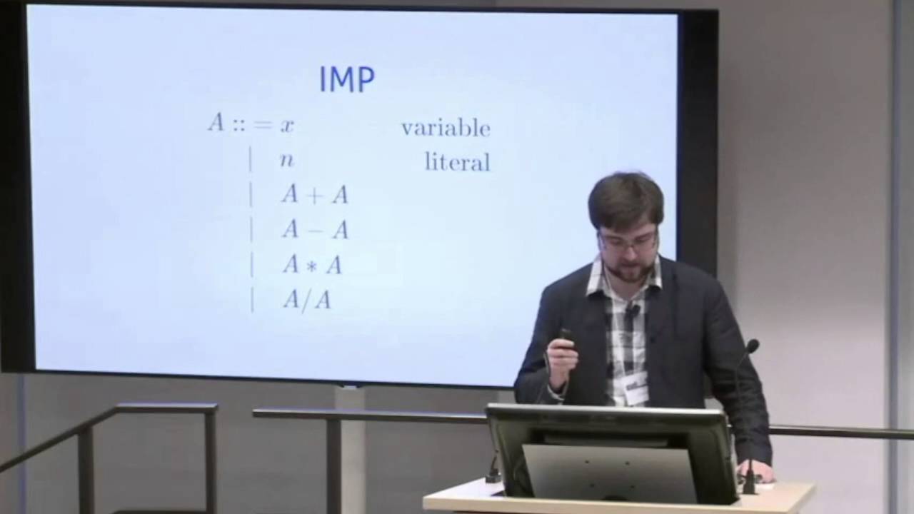
Tikhon Jelvis introduces the language he will be working with—a simple toy imperative language often known in the academic literature as Imp. The design goal is extreme minimalism: the simpler the source language can be kept, the simpler the formula compiler will be, making the whole analysis pipeline significantly easier to implement. Imp cleanly partitions execution into two distinct semantic categories: expressions and commands. Expressions evaluate strictly to values (either booleans or integers, which for simplicity are always represented as 32-bit integers) and are entirely free of side effects. Commands, on the other hand, produce no values whatsoever; their sole purpose is to produce side effects by mutating program state. The commands in Imp consist of variable assignments, `while` loops, conditional `if` statements, and sequential composition (`seq`) to chain commands together.
```mermaid flowchart TD accTitle: Imp Language Structural Split accDescr: Diagram showing the separation between pure expressions and state-modifying commands in the Imp language. subgraph Expressions["Expressions (Pure / Value-Producing)"] A["Arithmetic Expressions (AExpr)"] --> C["Produce Values (32-bit Ints / Bools)"] B["Boolean Expressions (BExpr)"] --> C C --> D["No Side Effects / Cannot Mutate Scope"] end subgraph Commands["Commands (Imp / State-Mutating)"] E["Assign (Set)"] --> H["Mutate State"] F["Conditionals (If) & Loops (While)"] --> H G["Sequencing (Seq) & No-Op (Skip)"] --> H H --> I["Produce No Value / Return Unit"] end ```
Traditionally, Imp is defined via an abstract grammar specifying arithmetic expressions with variables, literal constants, and standard arithmetic operators. Jelvis points out how naturally functional programming languages handle this representation: in Haskell, OCaml, or F#, abstract grammars translate almost directly into algebraic data types. The mapping is so direct that comparing the textbook BNF grammar to Haskell data constructors is almost trivial. For audience members less familiar with Haskell syntax, he highlights that constructors can be written as custom infix symbols (such as using `:+:` or `:-:`), mirroring mathematical notation. The grammar for commands follows the exact same pattern, introducing an explicit `Skip` constructor to serve as an empty block for things like empty branches in `if` statements.
- Expressions consist exclusively of side-effect-free evaluations of booleans and 32-bit signed/unsigned integers. - Commands change variable state and never return a value; they include assignment, sequencing, conditionals, loops, and no-ops (`Skip`). - The abstract grammar maps 1-to-1 onto algebraic data type definitions in Haskell.
---
[14:05](https://www.youtube.com/watch?v=ruNFcH-KibY&t=845s) Types as Skeletons and the Three Steps to SMT Compilation
Having established the data type for commands, Jelvis shares his mental model for compiler implementation: the algebraic type acts as a structural skeleton, while the implementation code is a layer of skin draped over it that naturally takes the skeleton's shape. Because the compiler functions pattern match against every constructor defined in the grammar, the overarching compilation challenge decomposes cleanly into small, isolated sub-problems. Rather than having to compile an entire monolithic language all at once, the developer simply solves the independent tasks of compiling `Skip`, compiling variable assignment (`Set`), compiling sequencing (`Seq`), and so on.
As Jelvis summarizes this decomposition strategy: “The way I like to visualize this is that the type is a sort of skeleton and the code is a sort of layer of skin which we lay on top of the skeleton and it naturally assumes that the shape that the types provide and this means that our problem is immediately broken up into a whole bunch of small pieces.”
Translating an imperative Imp program into an SMT-compatible logic formula requires three consecutive transformations: 1. **Inlining functions**: Any user-defined function calls are flattened by generating fresh variable names and substituting the function body directly at each call site—resembling the C preprocessor, though with proper hygienic naming. Unbounded recursion is handled by imposing a hard cutoff bound, matching the loop iteration bound. Once inlined, the compiler can treat the entire program as straight-line sequential code. 2. **Unrolling loops**: `while` loops are eliminated by unrolling them into nested conditional statements (`if` blocks) up to an arbitrary bound (such as 100 or 1,000 iterations, depending on the application). While this causes the textual footprint of the code to explode, modern SMT solvers process these large formulas surprisingly well. 3. **Single Static Assignment (SSA) conversion**: Because pure mathematical logic lacks an inherent notion of sequential time or programmatic mutation, the code must be translated into a purely declarative representation where every assignment creates a new versioned variable.
Jelvis adds a candid warning regarding SMT solver performance. Even among experts who have spent years writing and analyzing formulas with solvers like Z3, performance characteristics remain largely a black box. While size serves as a rough rule of thumb—larger formulas generally take longer to solve—solvers can behave counterintuitively, making performance difficult to predict when formulas differ in structure.
---
[17:27](https://www.youtube.com/watch?v=ruNFcH-KibY&t=1047s) Bridging Time and Logic: Single Static Assignment (SSA) and Phi Functions
The core intellectual challenge of compiling an imperative language into first-order logic lies in translating directionality. Programs execute step by step over time, with variables holding different values at different points. SMT formulas, however, have no chronological order; an SMT solver views a formula as a static, unordered collection of simultaneous constraints. Single Static Assignment (SSA) bridges this gap by creating an immutable, uniquely named variable for every variable mutation at each step in execution. For example, updating a variable $x$ generates constraints between versioned variables: $x_1 = x_0 + a_0$.
The primary difficulty with SSA arises when handling control-flow joins after conditional statements (`if` blocks). Because it cannot be determined statically which branch will execute at runtime, the variable $x$ could hold the value produced by the `then` branch ($x_1$) or the value produced by the `else` branch ($x_2$). Standard compiler theory solves this with a "phi function" ($\phi$), which acts like a magical oracle selecting the appropriate variable version based on which branch condition held true:
$$\phi(\text{condition}, x_1, x_2) = x_3$$
While SSA phi functions can feel like a compiler hack, they translate directly into conditional expressions inside SMT logic formulas.
---
[19:38](https://www.youtube.com/watch?v=ruNFcH-KibY&t=1178s) Compiling vs. Interpreting: The Scope and Z3 Assertions
Jelvis draws an illuminating parallel between writing an AST interpreter and writing a formula compiler for Z3: if you squint slightly, compiling an imperative language to SMT formulas looks nearly identical to writing an interpreter. Both architectures maintain a scope map to track variable states and both break down into three matching functions for arithmetic expressions, boolean expressions, and commands. However, the data returned by these functions diverges based on their objectives:
| Pipeline Component | Interpreter Return Type | Formula Compiler Return Type | |:--- |:--- |:--- | | **Arithmetic Expressions** | Evaluated concrete value (`Int`) | Unbound SMT AST fragment (Bit-vector AST) | | **Boolean Expressions** | Evaluated concrete value (`Bool`) | Unbound SMT AST fragment (Boolean AST) | | **Commands** | Updated scope mapping (`Scope`) | Solver state mutation / assertion (`Z3 ()`) |
In the interpreter, pure expressions evaluate directly into concrete primitives, whereas the SMT compiler produces syntax tree fragments that are not yet constraints on their own, but rather building blocks for larger formulas. In the interpreter, commands mutate and return a new scope environment. In the SMT compiler, executing a command pushes a logical assertion directly into Z3's state. As a result, the Imp command compiler in Haskell has the monadic return type `Z3 ()`. Jelvis jokes that to avoid excessive scope-checking plumbing in this presentation, he assumes all programmers write flawless code: “Similarly for the sake of simplicity I'm assuming that the programmer is perfect—yeah I am so fine—and that nobody ever makes any scope errors so I just you know the variable is always going to be in scope.”
---
[22:18](https://www.youtube.com/watch?v=ruNFcH-KibY&t=1338s) Explicit SMT Typing: Translating Bit Vectors
Moving into concrete code generation, Jelvis illustrates how an arithmetic expression such as `5 + x` compiles into an SMT formula. The compiler must translate this addition into bit-vector arithmetic, generating an AST node that adds two 32-bit bit vectors: an explicit 32-bit literal integer 5 and a 32-bit bit-vector variable representing the current SSA version of $x$ (for example, $x_0$).
Jelvis observes that SMT-LIB formulas require painful explicitness. Unlike high-level languages that infer representations or supply defaults, the SMT solver requires the compiler to specify exact bit widths for every literal and variable, as well as whether arithmetic operations are signed or unsigned. With this foundation established, compiling arithmetic expressions becomes an exhaustive pattern match over the AST constructors, emitting corresponding Z3 bit-vector primitives at every step.
[23:14](https://www.youtube.com/watch?v=ruNFcH-KibY&t=1394s) Compiling Expressions to Z3 Formulas
In a standard interpreter, evaluating a literal simply yields that raw number, and looking up a variable retrieves its final integer value from an evaluation scope. Compiling expressions into a Z3 formula follows an identical structural shape, but with symbolic targets. A literal integer becomes an explicit 32-bit bitvector node in the SMT abstract syntax tree. Similarly, the compiler’s scope maps source identifiers to symbolic variable names that the solver recognizes. When performing arithmetic operations such as addition, an interpreter simply recurses on both subexpressions and sums the results. In Z3, the translation is slightly more involved because the AST construction is managed inside a dedicated `Z3` monad in Haskell; the compiler must explicitly extract the results from the recursive monadic computations before constructing an addition AST node.
Arithmetic and boolean expressions follow this uniform structure across the board. Instead of generating addition nodes, operations like subtraction produce subtraction nodes, and boolean literals generate boolean solver nodes. Jelvis points out an aesthetic detail in his presentation code: he uses Unicode subscripts for indexed variables, which GHC accepts as valid Haskell identifiers. As Jelvis quips about configuring text editors: “You could actually use names like this in your code and you can configure Emacs to make it easy to type and then all non Emacs users will hate you but they had it coming.”
[25:00](https://www.youtube.com/watch?v=ruNFcH-KibY&t=1500s) Compiling Assignments and Managing State with Incremental Solving
Imperative state transitions, represented by assignment commands (`set`), require turning state modifications into assertions. Rather than mutating a memory cell, the compiler creates a fresh variable (such as $x_1$) and emits an assertion stating that this new variable equals the compiled representation of the right-hand side expression. Conceptually, compiling a sequence of statements produces a large conjunction of logical equality constraints. Handing these assertions to Z3 incrementally allows the solver to track them step-by-step rather than requiring the compiler to build a single massive `and` expression manually.
Breaking constraints into discrete assertions aligns naturally with incremental solving. When a solver operates incrementally, new constraints can be pushed onto an existing set of assertions without discarding the solver's internal state or invalidating previous reasoning. This enables users to refine specifications and add constraints efficiently without paying the performance penalty of re-solving from scratch. To implement this without maintaining manual integer counters (like $x_1, x_2, \dots$), the compiler relies on Z3’s built-in capability to generate distinct fresh variables from a given base name, keeping an internal lookup map so subsequent variable references resolve to the most recently generated fresh symbol.
- Variable assignment translates into allocating a fresh symbolic variable via Z3's native fresh variable API and asserting AST equality with the compiled right-hand side. - An internal scope map tracks the mapping from source-level identifier names to the latest active fresh Z3 symbol. - Incremental solving retains internal solver state across newly added assertions, avoiding full re-computation when adding assertions.
[27:52](https://www.youtube.com/watch?v=ruNFcH-KibY&t=1672s) Handling Branches with Symbolic If-Then-Else Expressions
Branching logic exposes the primary architectural difference between an interpreter and a symbolic formula compiler. An interpreter evaluates the guard condition and executes only the selected branch. A symbolic compiler cannot evaluate the guard at compile time, so it must compile both branches unconditionally. Reconciling the differing variable states produced by the two paths mirrors the $\phi$ (phi) functions used in Static Single Assignment (SSA) form. Z3 provides a direct equivalent through its native `ite` (if-then-else) symbolic expressions.
For every variable modified in either branch of an `if` statement, the compiler introduces a fresh variable defined by an `ite` assertion. The condition of the `ite` expression is the compiled boolean guard; if the condition holds, the solver chooses the variable instance resulting from the `then` branch, and if false, the instance from the `else` branch. Because loops were previously eliminated via bounded unrolling, the entire imperative language is reduced to just literals, assignments, and conditionals.
```mermaid flowchart TD accTitle: Branch compilation to SMT if-then-else accDescr: Diagram showing how both branches of an if statement compile simultaneously and merge via an ite node.
subgraph Inputs["Branch Analysis"] Cond["Compile Guard Condition: C"] B1["Compile Then-Branch: x_then"] B2["Compile Else-Branch: x_else"] end
subgraph SolverMerge["Z3 Phi Function"] ITE["Z3 Assert: x_fresh = ite(C, x_then, x_else)"] end
Cond --> ITE B1 --> ITE B2 --> ITE ```
[29:33](https://www.youtube.com/watch?v=ruNFcH-KibY&t=1773s) Bounded Model Checking and Temporal Invariants
Once an imperative program is compiled into a Z3 formula, it can be repurposed in several ways. While running it as a standard or reverse interpreter is mostly an entertaining sanity check, its primary analytical value lies in bounded model checking. Bounded model checking allows developers to specify program invariants using temporal logic, quantifying properties over execution time. Because loops have been unrolled into finite, discrete slices (represented by the sequence of SSA variable versions $x_1, x_2, x_3, \dots$), time is modeled as a discrete progression over execution steps.
Safety and liveness properties translate cleanly into boolean operations over these unrolled state slices: - An "always" temporal property ($\square P$) asserts that an invariant holds across every single iteration slice, compiling down to a large conjunction: $P(x_1) \land P(x_2) \land P(x_3) \land \dots$. - An "eventually" temporal property ($\lozenge P$) asserts that a condition will be satisfied at some point during execution, compiling down to a large disjunction: $P(x_1) \lor P(x_2) \lor P(x_3) \lor \dots$. - The temporal operators "always" and "eventually" act as duals, mapping onto the logical duality between conjunction (`and`) and disjunction (`or`).
[31:52](https://www.youtube.com/watch?v=ruNFcH-KibY&t=1912s) Program Verification and Inverted Satisfiability
To verify two programs against each other—such as checking an optimized implementation against an unoptimized reference specification—the solver checks whether there exists any valid input for which their outputs diverge. The compiler asserts that the inputs to both programs are identical while asserting that their final output variables are explicitly *not* equal:
$$\text{Assert: } \text{Output}_A \neq \text{Output}_B$$
When the solver runs on this formula, the interpretation of satisfiability is reversed relative to traditional test suites. If the solver reports `SAT` (satisfiable), the verification has failed: the solver found an assignment of inputs that produces differing outputs, yielding a concrete counterexample illustrating the bug. Conversely, if the solver returns `UNSAT` (unsatisfiable), the programs are proven equivalent within the unrolling bound because no input can cause them to disagree. Jelvis reflects on the mental hurdle this inversion presents: “Honestly this is a bit confusing at first because normally used you're used to the fact that something is satisfied means the result was true but here it's exactly the opposite.”
[32:27](https://www.youtube.com/watch?v=ruNFcH-KibY&t=1947s) Counterexample-Guided Program Synthesis and Optimization
Extending verification leads directly to program synthesis. By symbolically encoding program components—such as instruction choices, register slots, or AST operator nodes—as variables, the solver can search for an instruction sequence that matches desired input-output behaviors. Rather than solving for an exhaustive specification in one massive pass, synthesis uses counterexample-guided inductive synthesis (CEGIS).
The process operates as a feedback loop between a synthesizer and a verifier. First, the synthesizer finds a candidate program satisfying a single input-output pair. Because a single test case leaves room for incorrect edge-case behaviors, the candidate program is passed to the verifier, which attempts to find an input where the candidate diverges from the specification. When the verifier finds a counterexample, that input-output pair is fed back into the synthesizer. The synthesizer now finds a program that satisfies both constraints, and the loop repeats. While this loop might seem computationally prohibitive, each counterexample uncovers a fundamental algorithmic boundary or edge case, allowing the solver to prune vast swaths of the search space in remarkably few iterations. Jelvis highlights this as an ideal tool for code optimization: “In some sense this is like the most direct way to optimize something because we say well here's a program find a faster one and then the solver finds one.”
```mermaid flowchart LR accTitle: Counterexample-Guided Inductive Synthesis Loop accDescr: The iterative synthesis loop between a Z3 synthesizer and a Z3 verifier using counterexamples.
subgraph SynthesisLoop["CEGIS Iteration"] Synth["Synthesizer: Find program matching known points"] Verify["Verifier: Assert Program!= Spec"] end
Synth -->|"Candidate Program"| Verify Verify -->|"Counterexample (New Edge Case)"| Synth Verify -->|"UNSAT"| Verified["Verified Optimal Program"] ```
[34:15](https://www.youtube.com/watch?v=ruNFcH-KibY&t=2055s) Superoptimization and Program Sketching
Because SMT-driven program synthesis is computationally slow, running it on entire large programs is impractical. Instead, practical systems apply it over a sliding window across the code, behaving much like peephole optimization. Tikhon Jelvis argues that building an optimizer around an SMT solver can actually be far easier than writing an optimizing compiler like GCC from scratch because it eliminates the need to manually encode intricate optimization rules. As Jelvis explains: “I mean I can actually sort of say this confidently because I worked on a compiler that use this to optimize and there's no way I could have written all the rules by hand and in fact like I understood the architecture we were compiling to well enough to like simulate it but not well enough to write real programs by hand but that was totally fine because all we need is a formula compiler.”
Beyond peephole optimization, another technique to sidestep program size limits is program sketching. In this paradigm, developers already understand the high-level skeleton of their code—knowing where a loop, branch condition, or variable binding belongs—without knowing every implementation nuance. The programmer writes the code containing explicit "holes" alongside logical assertions, and an SMT-backed synthesizer automatically fills in the missing fragments to satisfy the constraints. Jelvis mentions an existing sketching compiler out of UC Berkeley designed for a Java-like language, but highlights a more compelling project called Synquid. Synquid takes refinement types (akin to Liquid Haskell) and automatically synthesizes complete function implementations directly from their type specifications, allowing users to experiment with type-driven synthesis online.
```mermaid flowchart TD accTitle: Program Synthesis Approaches accDescr: Diagram contrasting sliding window superoptimization and program sketching with SMT solvers.
subgraph Window["Sliding Window Superoptimization"] W1["Large Program Window"] --> W2["Sliding Peephole Slice"] W2 --> W3["Translate to SMT Formula"] W3 --> W4["Synthesize Optimized Fragment"] end
subgraph Sketch["Program Sketching"] S1["Program Skeleton with Holes"] S2["Refinement Types & Assertions"] S1 --> S3["SMT Solver Synthesis Engine"] S2 --> S3 S3 --> S4["Completed Valid Implementation"] end ```
[36:27](https://www.youtube.com/watch?v=ruNFcH-KibY&t=2187s) Developer Tooling and Domain-Specific Languages
SMT solvers offer broad utility across interactive developer workflows. They can model concurrency, construct execution traces during live coding (a technique known as angelic programming), and assist in debugging. A particularly high-leverage application is automated test case generation: since test suites are generated infrequently but executed repeatedly across continuous integration builds, developers do not need to worry if generating the test cases takes hours or even days. Additionally, synthesis techniques can power smarter code completion engines that infer intent and provide predictive suggestions directly within editors.
Implementing these systems for full-scale, general-purpose languages is immensely challenging because real-world programming languages are messy and complex. However, domain-specific languages (DSLs) represent the sweet spot for SMT tooling. DSLs are typically small, tightly scoped, and often lack features like unbounded loops or full Turing completeness. Because their operational boundaries are restricted by design, bounded verification can provide complete or practically sufficient guarantees. Furthermore, developers designing their own DSLs understand the language semantics intimately, making them far easier to formalize than general-purpose platforms.
- Jelvis initially studied these techniques in a graduate-level program synthesis course at UC Berkeley; although the professor moved to another institution, lecture slides and reference materials remain archived online. - Slides and bibliographic links to synthesis papers are hosted on Jelvis's personal site at `jelv.is/talks/compose-2016`. - Jelvis invites conference attendees to experiment with SMT solvers alongside him during the upcoming unconference weekend.
[39:50](https://www.youtube.com/watch?v=ruNFcH-KibY&t=2390s) Q&A: Real-World Specifications, Security Exploits, and Bit Vectors
During the audience Q&A, an attendee asks what problem specifications Jelvis used in his synthesis compiler. Jelvis explains that the project targeted an unusual, bespoke hardware architecture: rather than expressing specifications in high-level formal logic, the compiler simply took naively generated code fragments written in a low-level, specialized dialect of Forth and used those fragments directly as the semantic specification to synthesize faster, functionally equivalent code.
Another attendee from the security domain remarks that reverse interpreters could be immensely useful for generating malicious exploit payloads: knowing the expected exploit payload at an execution sink, a reverse interpreter could infer what input string must be supplied upstream to bypass filters. Jelvis acknowledges the utility while warning of unpredictable performance: running a program backward is fundamentally harder than executing it forward. However, SMT solvers often find satisfying counterexample inputs very quickly if one exists; the true computational bottleneck arises when trying to prove exhaustively that no exploit input exists. In practice, security analysts can impose a timeout: “...if you don't care about having like 100% verification you could just say well I'm going to run it for ten minutes and if it gives me a counter example it's good and if it doesn't well you know it's probably fine.”
An audience member comments on math foundations—noting that without conditional branches, program synthesis resembles polynomial or rational function interpolation in algebraic geometry, whereas adding branching conditionals requires cylindrical algebraic decomposition over the reals. Jelvis clarifies that his talk relied entirely on fixed-width bit vectors (such as standard 32-bit integers) rather than mathematical reals or unbounded integers. While SMT solvers include decision procedures for unbounded integers, doing so leads directly into undecidability and erratic performance profiles. Fixed-width bit vectors paired with bounded loop unrolling allow developers to enforce finite termination times while retaining practical verification capabilities.
## Mentioned Tikhon Jelvis, Z3, Microsoft Research, Haskell, OCaml, .NET, C#, F#, SBV, IMP, Liquid Haskell, QuickCheck, Synquid, GCC, UC Berkeley, Forth
## Video description Tikhon Jelvis C◦mp◦se :: Conference http://www.composeconference.org/ February 5, 2016
SMT solvers are widely used in research to analyze and verify programs. This lets us check invariants and compare programs against a spec exhaustively, with bounds on the number of loop iterations and the size of the heap. SMT solvers are also useful for other sorts of analysis including sophisticated type checking (like refinement types in Liquid Haskell) and fields other than program analysis (like security research where they can be used to analyze cryptographic algorithms and protocols).
I’ll demonstrate how to compile a simple language to an SMT formula and analyze programs using the Haskell Z3 bindings. Z3 has bindings in other languages including OCaml and .NET, so these ideas will be immediately useful to everyone even if the details are slightly different from the Haskell code. The underlying ideas will also help people approach other problems with Z3.
[Source](https://www.youtube.com/watch?v=ruNFcH-KibY)