3Blue1Brown Derives Backpropagation Gradients via Chain-Rule Sums
3Blue1Brown
Backpropagation calculates parameter updates by multiplying upstream neuron activations with downstream error sensitivities, requiring a sum across all outgoing pathways to propagate corrections recursively through earlier layers.
AI-assisted summary of Backpropagation calculus | Deep Learning Chapter 4 — original source. Check the original for full context.
Source published:
Key ideas
- Backpropagation formalizes the intuitive adjustment of weights and biases through the calculus chain rule, calculating how sensitive the final cost is to small nudges in each parameter along the computational pipeline. (0:38)
- The derivative of the cost with respect to a weight depends directly on the activation of the preceding neuron (∂z/∂w = a^(L-1)), mirroring the Hebbian learning principle that connections between active neurons undergo stronger updates. (3:56)
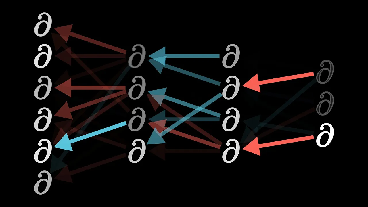
- Extending backpropagation to multi-neuron layers requires summing partial derivatives across all downstream neurons, because each neuron in a preceding layer influences the final cost through multiple simultaneous paths. (6:42)
- Evaluating cost sensitivity with respect to prior-layer activations (∂C₀/∂a^(L-1)) provides the necessary recursive bridge to propagate gradients backwards through the entire depth of the network. (5:39)
Detailed notes
## Background Published by 3Blue1Brown on YouTube on November 3, 2017, this video is the fourth chapter in the Deep Learning series. According to the page description, it offers a symbol-heavy, formal representation of the intuition behind backpropagation presented in part three, connecting conceptual animations to standard equations and codebase implementations.
## TL;DR Grant Sanderson derives the calculus of the backpropagation algorithm using a toy neural network where each layer contains a single neuron. By viewing the chain rule as a sequence of sensitivity ratios along a computational pipeline, he shows how to calculate the cost function's sensitivity with respect to weights, biases, and previous activations. He reveals that computing a single weight derivative constitutes most of the work, with prior neuron activations and prediction errors dictating weight adjustments in a manner mirroring Hebbian learning. Finally, he scales the formulation to multi-neuron architectures, showing that tracking indices and summing across parallel branching pathways enables identical equations to propagate recursively through the entire network.
## Atmosphere & style The presentation is patient, pedagogical, and calm, characterized by Grant Sanderson's trademark gentle and encouraging delivery. Despite tackling intimidating layers of subscripts and nested derivatives, the tone remains reassuring as viewers are urged to pause, ponder, and let the formalisms settle. It feels like an illuminating bridge between visual intuition and rigorous mathematical mechanics, culminating in a quiet sense of triumph upon uncovering the computational engine powering deep learning.
## Bulletin - [00:38](https://www.youtube.com/watch?v=tIeHLnjs5U8&t=38s) Backpropagation formalizes the intuitive adjustment of weights and biases through the calculus chain rule, calculating how sensitive the final cost is to small nudges in each parameter along the computational pipeline. - [03:56](https://www.youtube.com/watch?v=tIeHLnjs5U8&t=236s) The derivative of the cost with respect to a weight depends directly on the activation of the preceding neuron (∂z/∂w = a^(L-1)), mirroring the Hebbian learning principle that connections between active neurons undergo stronger updates. - [06:42](https://www.youtube.com/watch?v=tIeHLnjs5U8&t=402s) Extending backpropagation to multi-neuron layers requires summing partial derivatives across all downstream neurons, because each neuron in a preceding layer influences the final cost through multiple simultaneous paths. - [05:39](https://www.youtube.com/watch?v=tIeHLnjs5U8&t=339s) Evaluating cost sensitivity with respect to prior-layer activations (∂C₀/∂a^(L-1)) provides the necessary recursive bridge to propagate gradients backwards through the entire depth of the network.
## Key takeaways - [00:00](https://www.youtube.com/watch?v=tIeHLnjs5U8&t=0s) Chapter 4 aims to translate the high-level intuition of backpropagation from previous lessons into formal calculus and standard mathematical notation. - [00:38](https://www.youtube.com/watch?v=tIeHLnjs5U8&t=38s) Machine learning practitioners interpret the chain rule as a sequence of sensitivity ratios tracking how small nudges propagate through intermediate variables to the final cost. - [01:15](https://www.youtube.com/watch?v=tIeHLnjs5U8&t=75s) In a simplified single-neuron-per-layer network, superscripts are reserved for layer indexing, keeping subscripts available for individual neuron indexing in larger models. - [02:58](https://www.youtube.com/watch?v=tIeHLnjs5U8&t=178s) The chain rule expands the sensitivity of cost C₀ to weight w^(L) into three distinct factors: ∂z/∂w, ∂a/∂z, and ∂C₀/∂a. - [03:56](https://www.youtube.com/watch?v=tIeHLnjs5U8&t=236s) The derivative ∂C₀/∂a^(L) equals 2(a^(L) - y), scaling proportionally with the prediction error so larger mistakes induce stronger corrective updates. - [04:45](https://www.youtube.com/watch?v=tIeHLnjs5U8&t=285s) The derivative ∂z^(L)/∂w^(L) equals the activation of the preceding neuron a^(L-1), reflecting Hebbian learning where active inputs cause greater weight adjustments. - [05:15](https://www.youtube.com/watch?v=tIeHLnjs5U8&t=315s) The gradient for the overall network requires averaging individual cost derivatives across the entire training dataset or mini-batch. - [05:39](https://www.youtube.com/watch?v=tIeHLnjs5U8&t=339s) Deriving cost sensitivity with respect to a bias b^(L) uses the exact same chain structure, replacing the input factor with ∂z/∂b = 1. - [06:12](https://www.youtube.com/watch?v=tIeHLnjs5U8&t=372s) Computing the derivative of the cost with respect to preceding activation a^(L-1) is essential for recursively repeating the chain rule into earlier layers. - [06:42](https://www.youtube.com/watch?v=tIeHLnjs5U8&t=402s) Weight indexing uses w_jk^(L), listing the destination neuron j first and source neuron k second to align naturally with standard matrix-vector multiplication. - [08:25](https://www.youtube.com/watch?v=tIeHLnjs5U8&t=505s) In multi-neuron networks, a neuron's activation feeds forward into multiple destinations, requiring a summation across all connected neurons in the next layer to capture total cost sensitivity. - [09:13](https://www.youtube.com/watch?v=tIeHLnjs5U8&t=553s) Together, these iterative calculus expressions assemble the full gradient vector that guides gradient descent steps to minimize network error.
## Detailed walkthrough ### [00:00](https://www.youtube.com/watch?v=tIeHLnjs5U8&t=0s) Setting Up the Simple Network and the Chain Rule
Grant Sanderson begins by noting that this walkthrough assumes the viewer has watched chapter 3, which established the intuitive picture of the backpropagation algorithm. The purpose here is to formalize that intuition through calculus and notation, bridging the conceptual animations with the standard equations found in textbooks and code. He acknowledges that this material is dense and symbol-heavy: “It's normal for this to be at least a little confusing, so the mantra to regularly pause and ponder certainly applies as much here as anywhere else.” The perspective ML practitioners adopt toward the chain rule feels distinct from introductory calculus courses, viewing it as a sequence of sensitivity ratios along a computational pipeline.
```mermaid flowchart LR accTitle: Single Neuron Computational Flow accDescr: Computational pipeline showing how inputs, weights, and bias determine the intermediate value z, activation a, and cost C. subgraph LayerInputs["Inputs & Parameters"] A["a^(L-1)"] W["w^(L)"] B["b^(L)"] end subgraph ForwardPass["Forward Evaluation"] Z["z^(L)"] AL["a^(L)"] end subgraph LossEval["Evaluation"] Y["y (target)"] C["C_0 (Cost)"] end
A --> Z W --> Z B --> Z Z --> AL AL --> C Y --> C ```
To make the mechanics manageable, Sanderson strips the architecture down to a minimal toy model: a network where every layer contains exactly one neuron. Such a network with three hidden layers is governed by three weights and three biases. The goal is to see how sensitive the final cost is to adjustments in these parameters so the network can alter them to efficiently minimize error. Isolating the connection between the final two layers, the activation of the final neuron is labeled $a^{(L)}$ and the activation of the penultimate neuron is labeled $a^{(L-1)}$. Sanderson emphasizes that superscripts represent layer indices rather than algebraic exponents, keeping subscripts open for neuron indexing later.
For a single training example with desired target value $y$ (such as $0$ or $1$), the squared error cost is defined as $C_0 = (a^{(L)} - y)^2$. The final activation is produced by taking the weighted sum $z^{(L)} = w^{(L)} a^{(L-1)} + b^{(L)}$ and passing it through a non-linear activation function $\sigma$ (such as the sigmoid or ReLU), giving $a^{(L)} = \sigma(z^{(L)})$. Thinking of every variable as having its own number line, Sanderson traces the causal chain: a small nudge $\partial w^{(L)}$ causes an intermediate nudge $\partial z^{(L)}$, which triggers a nudge $\partial a^{(L)}$, which finally nudges $C_0$. Applying the chain rule translates this sequence into a product of three localized derivatives:
$$\frac{\partial C_0}{\partial w^{(L)}} = \frac{\partial z^{(L)}}{\partial w^{(L)}} \frac{\partial a^{(L)}}{\partial z^{(L)}} \frac{\partial C_0}{\partial a^{(L)}}$$
- **Target notation**: $y$ represents the ideal output value for a given training example. - **Cost expression**: $C_0 = (a^{(L)} - y)^2$ evaluates performance on that single example. - **Weighted input**: $z^{(L)} = w^{(L)} a^{(L-1)} + b^{(L)}$ bundles the linear combination before activation.
---
[03:56](https://www.youtube.com/watch?v=tIeHLnjs5U8&t=236s) Computing Derivatives and Their Intuitive Meaning
Sanderson breaks down each individual factor of the chain rule product to reveal what the algebra actually computes. Evaluating from the output backward: 1. The derivative of the cost with respect to the final activation is $\frac{\partial C_0}{\partial a^{(L)}} = 2(a^{(L)} - y)$. Its magnitude scales directly with the gap between the actual output and the desired target, meaning severe prediction errors produce large derivatives that exert strong corrective pressure. 2. The derivative of the activation with respect to the pre-activation input is $\frac{\partial a^{(L)}}{\partial z^{(L)}} = \sigma'(z^{(L)})$, simply the slope of the chosen activation function evaluated at $z^{(L)}$. 3. The derivative of the weighted sum with respect to the weight is $\frac{\partial z^{(L)}}{\partial w^{(L)}} = a^{(L-1)}$.
Sanderson urges viewers not to lose the big picture in the algebra: “In the case of this last derivative, the amount that the small nudge to the weight influenced the last layer depends on how strong the previous neuron is.” This directly reflects the classic Hebbian learning principle that neurons that fire together wire together: when the feeding neuron $a^{(L-1)}$ has a high activation, changing its connecting weight produces a far more pronounced effect on downstream computations.
He clarifies that this product gives the gradient component of the cost $C_0$ for just one training instance. Because the overall network cost function $C$ is the average of individual costs across all training examples, the true partial derivative with respect to any weight requires averaging that expression over the full dataset (or a mini-batch). This single term forms just one component of the full gradient vector, which packages the partial derivatives of the cost with respect to every single weight and bias across the entire network.
---
[05:39](https://www.youtube.com/watch?v=tIeHLnjs5U8&t=339s) Sensitivity to Biases and Propagating Backward
Even though calculating one weight derivative seems like a tiny fraction of the whole network, Sanderson points out that “even though that's just one of the many partial derivatives we need, it's more than 50% of the work.” Determining sensitivity to the bias $b^{(L)}$ requires swapping only the final term in the chain: replacing $\frac{\partial z^{(L)}}{\partial w^{(L)}}$ with $\frac{\partial z^{(L)}}{\partial b^{(L)}}$. Because $z^{(L)} = w^{(L)} a^{(L-1)} + b^{(L)}$, the partial derivative with respect to $b^{(L)}$ evaluates to $1$:
$$\frac{\partial C_0}{\partial b^{(L)}} = \frac{\partial z^{(L)}}{\partial b^{(L)}} \frac{\partial a^{(L)}}{\partial z^{(L)}} \frac{\partial C_0}{\partial a^{(L)}} = 1 \cdot \sigma'(z^{(L)}) \cdot 2(a^{(L)} - y)$$
```mermaid flowchart TD accTitle: Backpropagation Iteration Cycle accDescr: Flow diagram showing how cost sensitivity flows from Layer L activations back to weights, biases, and the prior layer activations. subgraph LayerL["Layer L Derivatives"] dC_daL["∂C₀ / ∂a^(L)"] dC_dzL["∂C₀ / ∂z^(L) = σ'(z^(L)) · ∂C₀ / ∂a^(L)"] end subgraph LayerLParams["Parameter Updates"] dW["∂C₀ / ∂w^(L) = a^(L-1) · ∂C₀ / ∂z^(L)"] dB["∂C₀ / ∂b^(L) = 1 · ∂C₀ / ∂z^(L)"] end subgraph PriorLayer["Propagation Step"] dC_daLprev["∂C₀ / ∂a^(L-1) = w^(L) · ∂C₀ / ∂z^(L)"] end
dC_daL --> dC_dzL dC_dzL --> dW dC_dzL --> dB dC_dzL --> dC_daLprev ```
Crucially, this framework also reveals how sensitive the cost function is to the activation of the preceding neuron, $\frac{\partial C_0}{\partial a^{(L-1)}}$. Evaluating the initial sensitivity of $z^{(L)}$ to $a^{(L-1)}$ yields the weight itself: $\frac{\partial z^{(L)}}{\partial a^{(L-1)}} = w^{(L)}$. While the network cannot directly tweak an activation value—since activations are determined strictly by earlier layers—computing this sensitivity is essential. It serves as the launchpad for the recursive step: once the sensitivity to $a^{(L-1)}$ is known, the exact same chain rule pattern propagates backwards to assess sensitivity to all preceding weights $w^{(L-1)}$ and biases $b^{(L-1)}$.
---
[06:42](https://www.youtube.com/watch?v=tIeHLnjs5U8&t=402s) Scaling to Layers with Multiple Neurons
Moving from a single-neuron chain to real networks with multiple neurons per layer might seem daunting, but Sanderson reassures the viewer that “honestly, not that much changes when we give the layers multiple neurons, really it's just a few more indices to keep track of.” In a multi-neuron architecture: - Subscript $k$ indexes neurons in the prior layer $L-1$. - Subscript $j$ indexes neurons in the current layer $L$. - The activation of the $j$-th neuron in layer $L$ is written as $a_j^{(L)}$. - The connection strength between neuron $k$ in layer $L-1$ and neuron $j$ in layer $L$ is designated $w_{jk}^{(L)}$.
Sanderson admits that indexing the weight as $w_{jk}^{(L)}$ (destination index first, source index second) can feel backward at first glance, but explains that this convention is deliberate: it matches standard matrix multiplication, where row $j$ of a weight matrix multiplies the activation vector to produce the $j$-th entry of the output.
```mermaid flowchart LR accTitle: Multi-Neuron Branching Influence accDescr: Diagram illustrating how a single neuron in layer L-1 branches out to influence multiple neurons in layer L, requiring a summation in backprop. subgraph LayerPrev["Layer L-1"] ak["a_k^(L-1)"] end subgraph LayerCurr["Layer L"] zj0["z_0^(L)"] --> aj0["a_0^(L)"] zj1["z_1^(L)"] --> aj1["a_1^(L)"] end subgraph FinalCost["Cost Function"] Cost["C_0 = Σ (a_j^(L) - y_j)²"] end
ak -->|"w_0k^(L)"| zj0 ak -->|"w_1k^(L)"| zj1 aj0 --> Cost aj1 --> Cost ```
The overall cost function for a single example sums the squared errors across all output neurons:
$$C_0 = \sum_{j} (a_j^{(L)} - y_j)^2$$
The pre-activation weighted sum for neuron $j$ is $z_j^{(L)} = \sum_k w_{jk}^{(L)} a_k^{(L-1)} + b_j^{(L)}$, followed by $a_j^{(L)} = \sigma(z_j^{(L)})$. The derivative of the cost with respect to an individual weight $w_{jk}^{(L)}$ maintains an identical structure to the single-neuron case:
$$\frac{\partial C_0}{\partial w_{jk}^{(L)}} = \frac{\partial z_j^{(L)}}{\partial w_{jk}^{(L)}} \frac{\partial a_j^{(L)}}{\partial z_j^{(L)}} \frac{\partial C_0}{\partial a_j^{(L)}} = a_k^{(L-1)} \cdot \sigma'(z_j^{(L)}) \cdot 2(a_j^{(L)} - y_j)$$
The key mathematical difference appears when computing the derivative with respect to an activation in the previous layer, $a_k^{(L-1)}$. Because activation $a_k^{(L-1)}$ branches out and feeds into every neuron in layer $L$, it influences the cost function through multiple distinct pathways simultaneously. To capture its total impact, the sensitivities through each pathway must be summed together:
$$\frac{\partial C_0}{\partial a_k^{(L-1)}} = \sum_j \frac{\partial z_j^{(L)}}{\partial a_k^{(L-1)}} \frac{\partial a_j^{(L)}}{\partial z_j^{(L)}} \frac{\partial C_0}{\partial a_j^{(L)}} = \sum_j w_{jk}^{(L)} \cdot \sigma'(z_j^{(L)}) \cdot \frac{\partial C_0}{\partial a_j^{(L)}}$$
Once this aggregated sensitivity for each neuron $k$ in layer $L-1$ is computed, the exact same equations iterate backwards through the entire depth of the network. Sanderson celebrates reaching this milestone: “If all of this makes sense, you have now looked deep into the heart of backpropagation, the workhorse behind how neural networks learn.” These mathematical expressions systematically populate the gradient vector, providing the exact numerical direction needed to minimize cost by repeatedly stepping downhill. He concludes with an encouraging note to let the concepts settle, acknowledging that tracking these nested layers of indices and derivatives takes time to fully digest.
## Notable quotes > [06:42](https://www.youtube.com/watch?v=tIeHLnjs5U8&t=402s) honestly, not that much changes when we give the layers multiple neurons, really it's just a few more indices to keep track of. — Grant Sanderson
## Mentioned 3Blue1Brown, Grant Sanderson, Vincent Rubinetti, Влад Бурмистров, Omer Tuchfeld, ReLU, Sigmoid
## Video description Help fund future projects: https://www.patreon.com/3blue1brown An equally valuable form of support is to share the videos. Special thanks to these supporters: http://3b1b.co/nn3-thanks Written/interactive form of this series: https://www.3blue1brown.com/topics/neural-networks
This one is a bit more symbol-heavy, and that's actually the point. The goal here is to represent in somewhat more formal terms the intuition for how backpropagation works in part 3 of the series, hopefully providing some connection between that video and other texts/code that you come across later.
For more on backpropagation: http://neuralnetworksanddeeplearning.com/chap2.html https://github.com/mnielsen/neural-networks-and-deep-learning http://colah.github.io/posts/2015-08-Backprop/
Music by Vincent Rubinetti: https://vincerubinetti.bandcamp.com/album/the-music-of-3blue1brown
Thanks to these viewers for their contributions to translations Звуковая дорожка на русском языке: Влад Бурмистров. Hebrew: Omer Tuchfeld
------------------ Video timeline 0:00 - Introduction 0:38 - The Chain Rule in networks 3:56 - Computing relevant derivatives 4:45 - What do the derivatives mean? 5:39 - Sensitivity to weights/biases 6:42 - Layers with additional neurons 9:13 - Recap ------------------
3blue1brown is a channel about animating math, in all senses of the word animate. And you know the drill with YouTube, if you want to stay posted on new videos, subscribe, and click the bell to receive notifications (if you're into that): http://3b1b.co/subscribe
If you are new to this channel and want to see more, a good place to start is this playlist: http://3b1b.co/recommended
Various social media stuffs: Website: https://www.3blue1brown.com Twitter: https://twitter.com/3Blue1Brown Patreon: https://patreon.com/3blue1brown Facebook: https://www.facebook.com/3blue1brown Reddit: https://www.reddit.com/r/3Blue1Brown
[Source](https://www.youtube.com/watch?v=tIeHLnjs5U8)