Mill Scraps Registers for Conveyor Belt to Cut Processor Power Drain
The Mill CPU Architecture - the Belt (2 of 13) — Mill Computing, Inc.

Mill Computing, Inc.

Replacing traditional register files with a temporal conveyor belt eliminates renaming hardware and slashes bypass multiplexer sources, enabling 33 operations per cycle at digital signal processor efficiency levels.

AI-assisted summary of The Mill CPU Architecture - the Belt (2 of 13) — original source. Check the original for full context.

Source published:

Key ideas

  • Mill Computing introduced the Belt, an alternative CPU operand model that replaces conventional register files and dynamic register renaming with a temporal FIFO queue. (20:55)
  • By shifting from spatial registers to temporal addressing, the Mill core slashes routing sources from approximately 450 to 64, cutting the interconnect power overhead that accounts for nearly half of modern superscalar consumption. (32:28)
  • The flagship Mill Gold configuration targets 33 MIMD operations per cycle at 1.2 GHz and 28 W, offering up to 80 GOPS peak through compiler-driven exposed-pipeline scheduling. (3:12)
  • Software compatibility across diverse Mill microarchitectures is achieved via an install-time specialization model derived from IBM AS/400 rather than fixed instruction bit patterns. (76:05)

Detailed notes

## Background Published on YouTube by Mill Computing, Inc. on July 29, 2013, this video is the second installment in a 13-part lecture series detailing the company's novel CPU architecture. The presentation focuses on the Belt, introducing a conveyor-belt machine model designed to eliminate register renaming, false hazards, and bypass routing overhead.

## TL;DR Ivan Godard presents the Mill CPU architecture and its central mechanism, the Belt, which replaces conventional general-purpose registers with a temporal FIFO structure where functional unit outputs drop at the front and age off the back. He illustrates how standard out-of-order superscalar processors squander over 90 percent of their power and silicon area on register renaming and massive bypass multiplexer trees to handle transient data. By exposing execution latencies directly to the compiler and leveraging temporal addressing, the Mill eliminates write-after-read and write-after-write hazards, drops instruction destination encodings, and achieves up to 33 MIMD operations per cycle at DSP-level energy efficiency.

## Atmosphere & style The presentation carries the dynamic feel of an advanced Silicon Valley engineering colloquium, marked by dry humor, intellectual candor, and technical irreverence. Ivan Godard speaks with the easy confidence of a veteran systems architect, poking fun at industry conventions and openly conceding the design's trade-offs and 'vaporware' status with lines like admitting he is 'lying through his teeth' to simplify complex multiplexer math. The mood is intellectually stimulating and grounded, transforming abstract microarchitectural theory into a lively, first-principles critique of mainstream processor design.

## Bulletin - [20:55](https://www.youtube.com/watch?v=QGw-cy0ylCc&t=1255s) Mill Computing introduced the Belt, an alternative CPU operand model that replaces conventional register files and dynamic register renaming with a temporal FIFO queue. - [32:28](https://www.youtube.com/watch?v=QGw-cy0ylCc&t=1948s) By shifting from spatial registers to temporal addressing, the Mill core slashes routing sources from approximately 450 to 64, cutting the interconnect power overhead that accounts for nearly half of modern superscalar consumption. - [03:12](https://www.youtube.com/watch?v=QGw-cy0ylCc&t=192s) The flagship Mill Gold configuration targets 33 MIMD operations per cycle at 1.2 GHz and 28 W, offering up to 80 GOPS peak through compiler-driven exposed-pipeline scheduling. - [01:16:05](https://www.youtube.com/watch?v=QGw-cy0ylCc&t=4565s) Software compatibility across diverse Mill microarchitectures is achieved via an install-time specialization model derived from IBM AS/400 rather than fixed instruction bit patterns.

## Key takeaways - [06:33](https://www.youtube.com/watch?v=QGw-cy0ylCc&t=393s) Modern superscalar processors expend over 90% of their power and silicon area on control logic, prediction, renaming, and bypass crossbars rather than actual computation. - [11:20](https://www.youtube.com/watch?v=QGw-cy0ylCc&t=680s) Bypass crossbars on architectures like Intel Haswell require routing paths among roughly 500 sources and 100 sinks, scaling multiplexer latency and consuming about half of the total core power. - [18:28](https://www.youtube.com/watch?v=QGw-cy0ylCc&t=1108s) Empirical studies by Yale Patt indicate that 80% of temporary values are referenced only once, serving strictly as point-to-point dataflow connections between instructions. - [20:55](https://www.youtube.com/watch?v=QGw-cy0ylCc&t=1255s) The Belt provides a conveyor-belt machine model using relative temporal addressing (B0, B1, etc.) where newest results enter at the front and older values naturally drop off. - [20:55](https://www.youtube.com/watch?v=QGw-cy0ylCc&t=1255s) Temporal addressing eliminates explicit destination register fields in instruction encodings, significantly shrinking machine code size. - [23:56](https://www.youtube.com/watch?v=QGw-cy0ylCc&t=1436s) Values that must survive past their belt residency are transferred into a non-addressable, frame-local SRAM scratchpad using static-offset spill and fill operations. - [27:01](https://www.youtube.com/watch?v=QGw-cy0ylCc&t=1621s) Operations producing multiple results, such as division generating both quotient and remainder, drop both outputs onto the belt in one cycle without special registers or glitches. - [28:24](https://www.youtube.com/watch?v=QGw-cy0ylCc&t=1704s) Function calls and returns execute in a single cycle with zero prologue or epilogue overhead, passing arguments directly on the belt and returning intact caller state. - [35:00](https://www.youtube.com/watch?v=QGw-cy0ylCc&t=2100s) Mill pipelines expose exact execution latencies to the compiler, allowing multi-cycle operations to remain in flight across calls and retire directly into their issuing frame. - [40:26](https://www.youtube.com/watch?v=QGw-cy0ylCc&t=2426s) Hardware interrupts are handled identically to spontaneous, involuntary function calls, avoiding duplicate supervisor registers or destructive pipeline flushes. - [42:17](https://www.youtube.com/watch?v=QGw-cy0ylCc&t=2537s) A two-stage segregated crossbar interconnect directly couples single-cycle ALUs while routing multi-cycle functional units through a secondary network, reducing multiplexer depth to 1–2 levels. - [01:00:39](https://www.youtube.com/watch?v=QGw-cy0ylCc&t=3639s) Advancing the belt is implemented by broadcasting an index offset increment across tagged output registers rather than physically shifting data between flip-flops. - [55:56](https://www.youtube.com/watch?v=QGw-cy0ylCc&t=3356s) Security and privilege rings are eliminated; protection is enforced purely through memory addressing boundaries, dispensing with supervisor modes and privileged instructions. - [01:16:05](https://www.youtube.com/watch?v=QGw-cy0ylCc&t=4565s) Programs are distributed as an abstract intermediate representation and specialized into native machine instructions at installation to adapt to specific belt sizes and issue widths. - [01:19:28](https://www.youtube.com/watch?v=QGw-cy0ylCc&t=4768s) Aggressive software pipelining and if-conversion allow complex control flows like the Unix wc loop to compile into branchless single-cycle kernels issuing up to 25 operations concurrently.

## Detailed walkthrough ### [00:00](https://www.youtube.com/watch?v=QGw-cy0ylCc&t=0s) Introduction and the Tale of Two Architectures

Ivan Godard opens the talk by thanking Google for providing the venue and the invitation. He introduces this lecture as part of an ongoing series detailing the Mill general-purpose CPU architecture, focusing specifically on internal data structures, inter-operation data communication, the programmer's execution model, and an overview of the underlying physical implementation.

To frame the problem, he contrasts two contemporary top-of-the-line processors from major manufacturers representing polar opposite design philosophies: 1. **Out-of-Order Superscalar CPU:** A 4-core desktop/server chip operating at 3.3 GHz, issuing a peak of 4 operations per cycle per core. It consumes 130 W, delivers 52 giga-operations per second (GOPS), and sells for $885 in quantities of 1,000. 2. **In-Order VLIW DSP:** A single-core embedded digital signal processor operating at 500 MHz (0.5 GHz) that issues 8 operations per cycle peak. It consumes a mere 1.1 W, delivers 3.6 giga-instructions per second (GIPS), and costs only $17 in 1,000-unit quantities.

Comparing their power and cost efficiencies reveals a staggering gap: the out-of-order superscalar provides 406 MIPS per watt and 59 MIPS per dollar, whereas the in-order DSP operates in a completely different efficiency realm. Normalizing the comparison to a per-core basis underscores this penalty: the superscalar core provides roughly 3.5× higher performance than the DSP core, but it costs 30× as much power and 13× as much money.

| Metric | Out-of-Order Superscalar (4 cores) | In-Order VLIW DSP (1 core) | Superscalar vs DSP (Per-Core Ratio) | |:--- |:--- |:--- |:--- | | **Clock Frequency** | 3.3 GHz | 0.5 GHz (500 MHz) | ~6.6× frequency | | **Peak Issue Width** | 4 ops/cycle/core | 8 ops/cycle/core | 0.5× issue width | | **Power Dissipation** | 130 W total (~32.5 W/core) | 1.1 W | ~30× power per core | | **Throughput** | 52 GOPS total (13 GOPS/core) | 3.6 GIPS | ~3.6× performance per core | | **1k Unit Price** | $885 (~$221/core) | $17 | ~13× cost per core | | **Power Efficiency** | 406 MIPS/W | High DSP efficiency | Severe superscalar penalty | | **Cost Efficiency** | 59 MIPS/$ | High DSP efficiency | Severe superscalar penalty |

---

[03:12](https://www.youtube.com/watch?v=QGw-cy0ylCc&t=192s) The Efficiency Disparity and the Mill Objective

Addressing why such a dramatic commercial disparity persists without being arbitraged away, Godard explains that the DSP is a 32-bit architecture whereas the superscalar is a 64-bit machine. Furthermore, users seeking absolute single-thread horsepower cannot extract it from a DSP. Most crucially, their target workloads are fundamentally incompatible: “Signal processing is just not the same as general purpose code.” A DSP VLIW tasked with running a typical general-purpose desktop operating system and software would perform terribly. Conversely, running DSP workloads on a superscalar is technically feasible, but only “as long as you had enough Freon to keep it cool.”

The founding challenge for Mill Computing was to bridge this gap: achieve DSP-level energy and cost efficiency on general-purpose software workloads. Following nearly a decade of research and development, Godard presents the projected figures for the **Mill Gold**: - **Configuration:** 2 cores on a single chip. - **Issue Width:** 33 operations per cycle peak per core. - **Clock Frequency:** 1.2 GHz (roughly one-third the clock rate of high-end superscalars). - **Power Consumption:** 28 W. - **Throughput:** Just under 80 GOPS peak. - **Projected Price:** $225.

Godard is candid about the current status of the project: “Now, this is vaporware. We are several years still away from having something with pins on the bottom.” The power numbers represent engineering estimates derived from multi-year cycle-accurate simulations, while the projected price is an estimate given that they intentionally operate without a marketing department: “and the longer that lasts, the happier I'll be.”

Comparing the Mill Gold core against the baseline processors shows: - **Mill vs. DSP (per core):** The Mill achieves 11× the performance at 12× the power, demonstrating successful linear scaling of DSP-like efficiency up to high performance. - **Mill vs. Superscalar (per core):** The Mill achieves nearly 2.5× the performance while requiring nearly 2.5× less power and costing roughly half the price.

---

[06:33](https://www.youtube.com/watch?v=QGw-cy0ylCc&t=393s) 33 Operations per Cycle: Why and How?

No existing production processor issues 33 operations per cycle. Godard clarifies that these 33 operations are independent MIMD instructions—not SIMD lanes or packed vector elements where operations inside a vector are inflated into separate counts. If the Mill counted SIMD execution that way, the Gold configuration would claim over 500 operations per cycle peak. Instead, these are 33 distinct, concurrent instructions—branches, loads, adds, and logical operations—that strictly match the chip's functional unit population. On the Gold core, this includes up to 8 integer adds simultaneously alongside other operations.

Explaining why 33-wide issue is desirable, Godard points out that the vast majority of executed instructions reside inside loops. DSP loops are conventionally software pipelined, and software pipelines possess unbounded instruction-level parallelism (ILP). While realized instructions per cycle (IPC) is capped by the number of physical functional units (such as available adders), the potential ILP in loops is enormous. General-purpose loops rarely achieve software pipelining on conventional architectures due to control flow, branches, and function calls.

```mermaid flowchart TD accTitle: Superscalar Resource Breakdown accDescr: Diagram illustrating that functional units occupy only eight to nine percent of superscalar area and power while control and data distribution consume the rest. subgraph ChipBudget["Superscalar Area & Power Budget"] direction TB Control["Control & Data Routing (~91-92%)<br/>• Next-op prediction<br/>• Instruction decode & dispatch<br/>• Execution staging<br/>• Result bypass crossbars"] ALUs["Execution Units (~8-9%)<br/>• Adders, multipliers<br/>• Vector units, shufflers"] end ```

The Mill incorporates architectural mechanisms allowing software pipelining across nearly all loops, including those with embedded calls and irregular branches, driving loop execution overhead down below 15% of cycles. This approach pays off because functional units are cheap: - “An adder is a tiny, tiny little thing.” - On modern processors, all functional units combined (adders, shifters, multipliers, vector engines) account for only 8% to 9% of total chip area and power dissipation. - Nearly the entire area and energy budget of an out-of-order superscalar is squandered on overhead: determining what to execute next, preparing operands, and dynamically routing results to subsequent consumers.

Adding vast arrays of functional units is straightforward and cheap. The real bottlenecks to achieving a 33-issue machine are instruction decoding and data distribution. Godard notes that the decode mechanism—handling variable-length, x86-like instruction bundles at 33 operations per cycle—was addressed in a previous talk at Stanford's EE 380 seminar. The central problem of this lecture is data routing: how to feed data between operations at a rate exceeding 30 operations every single cycle.

---

[11:20](https://www.youtube.com/watch?v=QGw-cy0ylCc&t=680s) The Interconnect Explosion: Sources, Sinks, and Multiplexers

Godard cautions that hardware descriptions at this level are an intentional simplification to provide an intuitive understanding of the engineering challenge: “Any of you who actually do do chip design know I'm lying through my teeth, but at least you'll get a sense of the order of magnitude of the problem.” Modern out-of-order processors suffer from an extreme producer-consumer fan-out problem: - In an architecture like Intel Haswell, there are nearly 500 distinct internal data sources (functional unit outputs, rename registers, bypass buffers). - Haswell contains nearly 100 data sinks (functional unit operand ports, reservation stations, memory queues). - Supporting universal routing—allowing any source to feed any sink across full data-path widths—requires an interconnect fabric with up to 50,000 possible cross-point connections.

```mermaid flowchart LR accTitle: Source to Sink Multiplexer Tree Routing accDescr: Diagram showing how multiple data sources are selected via multiplexer trees driven by control lines to feed a single consumer sink. subgraph Sources["Sources (~500 on Haswell)"] S0["Source 0"] S1["Source 1"] S2["Source..."] SN["Source 499"] end

subgraph MuxTree["Multiplexer Tree"] M1["Mux Layer 1"] M2["Mux Layer 2"] MFinal["Final Mux"] Ctrl["Control Lines"] -.-> M1 Ctrl -.-> M2 Ctrl -.-> MFinal end

subgraph Sink["Operand Sink (~100 total)"] Consumer["Functional Unit Input"] end

S0 --> M1 S1 --> M1 S2 --> M2 SN --> M2 M1 --> MFinal M2 --> MFinal MFinal --> Consumer ```

The fundamental circuit component used to route this data is the 2-to-1 multiplexer (mux). It takes two data inputs at the top, a control select line at the side, and routes one chosen input to its single output. To feed a single sink from hundreds of candidate sources, designers cascade multiplexers into large decoding trees. The control logic configures the select signals across each layer of the tree, guiding the appropriate data word down through the levels of logic until it lands at the destination functional unit input port. Scaling this conventional bypass network up to 33 issue slots causes an unmanageable explosion in multiplexer complexity, wire routing congestion, latency, and power dissipation.

[13:59](https://www.youtube.com/watch?v=QGw-cy0ylCc&t=839s) The Interconnect Tax: Latency, Power, and the Superscalar Limit

Even simplifying away the intricate hardware implementations down to multiplexer trees, the physics of connecting functional units together remains unforgiving. Latency—the time required to route data from a producer source to a consumer sink—scales with the depth of the connection path, which is logarithmic to the number of sources. Power consumption is even harsher, scaling roughly with the product of sources and sinks. A pool of roughly 500 sources yields nine multiplexer levels, adding at least three whole pipeline stages just to traverse the bypass network. The real-world consequence inside modern high-performance superscalars is staggering: on a chip like Intel's Haswell, routing data through this internal interconnect network consumes approximately half of the core's total electrical power.

Engineers have devised countless clever workarounds and routing topologies over decades of chip design, many of which ship in commercial processors today. Yet while these mitigations help around the edges, they cannot alter the fundamental scaling problem. A traditional VLIW processor can achieve high compute density at a fraction of the energy because it only needs to route around eight sources, whereas an aggressive superscalar routes among hundreds. The ceiling on modern processing performance is not functional unit math, but the raw power and timing budget required for data distribution.

> “And when it all comes down to it, this interconnect tends to on a superscalar such as the Haswell will tend to consume around half of the overall power of the chip of the core.”

- **Latency scaling**: Proportional to connection depth, or $\log_2(\text{sources})$; 500 sources require 9 multiplexer levels, adding at least 3 pipeline stages. - **Power scaling**: Proportional to $\text{sources} \times \text{sinks}$. - **Architecture comparison**: Superscalars pay roughly 30 times the interconnect power penalty of an 8-source VLIW machine. - **Root barrier**: The primary performance ceiling is the power-times-delay cost of operand delivery.

---

[15:34](https://www.youtube.com/watch?v=QGw-cy0ylCc&t=934s) Hazards and Register Renaming: Why Processors Need 500 Sources

The sheer volume of sources raises an obvious paradox: if an instruction set architecture only defines 32 architectural registers, why do modern chips contain hundreds of physical sources? The culprit is register renaming. When a naive compiler translates two completely independent source code statements into machine instructions, it frequently reuses temporary registers. For example, if expression one computes an addition into temporary register `RT` and increments it, while expression two independently computes a subtraction into `RT` and adds to it, there is no genuine data dependency between the two calculations. In theory, both initial operations could execute concurrently in cycle one, and both finishing operations could execute in cycle two.

```mermaid flowchart TD accTitle: False Dependency Hazard vs Register Renaming accDescr: Diagram contrasting how reusing temporary register RT creates a hazard, which hardware resolves by renaming to RT1 and RT2.

subgraph Hazard ["Architectural Register Hazard"] direction TB H1["Cycle 1: Add -> RT"] H2["Cycle 1: Sub -> RT"] HZ{{"Hazard: Which RT value survives?"}} H1 --> HZ H2 --> HZ end

subgraph Renamed ["Hardware Register Renaming"] direction TB R1["Cycle 1: Add -> RT1"] R2["Cycle 1: Sub -> RT2"] R3["Cycle 2: Inc RT1 -> Res1"] R4["Cycle 2: Add RT2 -> Res2"] R1 --> R3 R2 --> R4 end ```

The problem arises at the cycle boundary: if both instructions assign to `RT` simultaneously, the processor encounters a write-after-write hazard. When the subsequent instructions reference `RT`, the hardware cannot know which value to read, risking a bit-merged corruption of both results. To allow parallel execution without stalling, out-of-order processors dynamically remap those architectural register names onto a vast internal pool of rename registers, converting `RT` into distinct physical registers `RT1` and `RT2`. Compilers are forced into this reuse because 32 registers are insufficient, architectures lack clean mechanisms to mark when an operand has seen its final use, and calling conventions obscure whether downstream functions will preserve register contents.

> “This is called a hazard, and rename is a device used to avoid hazard in processors.”

- **The false dependency problem**: Compilers running out of registers emit false write-after-write (WAW) and write-after-read (WAR) dependencies between unrelated expressions. - **Hardware renaming overhead**: The CPU must dynamically track and rename architectural names into separate physical registers so instructions can issue in parallel. - **The compiler's dilemma**: Compilers cannot easily communicate the "last use" of an operand, forcing hardware to conservatively keep register allocations alive.

---

[18:28](https://www.youtube.com/watch?v=QGw-cy0ylCc&t=1108s) The Anatomy of Temporaries and the Failure of Stacks

Analyzing how programs actually utilize temporary registers exposes how mismatched conventional register files are to actual execution needs. Academic research conducted by Yale Patt and one of his students revealed that an overwhelming 80% of all temporary values are referenced exactly once. These single-use values exist for no other reason than to serve as ephemeral plumbing—forwarding the output of an adder into the input of a multiplier, never to be touched again. A modest 14% of values are referenced two or more times, behaving as true local fast memory to stash data for short-term reuse. The remaining 6% of produced temporaries are never referenced at all.

Instead of forcing a single, bloated register mechanism to handle both dataflow plumbing and temporary storage, an architecture ought to decouple them. Historical architectures managed dataflow without named general registers: accumulator machines implicitly used the accumulator for results and inputs, eliminating hazards at the cost of strict serialization. Stack machines similarly took both inputs from the top of the stack and pushed results back, naturally avoiding hazards and renaming. However, because a classic stack machine only exposes a single stack top, it can only execute a single operation at a time, entirely defeating wide instruction issue. The ideal machine model requires several interleaved stacks whose entries can be accessed by multiple functional units simultaneously.

> “80% are referenced exactly once. They are used solely to indicate the data flow connection from one operation to another.”

- **Yale Patt temporary value distribution**: - **80% single-use**: Pure dataflow connections between operations. - **14% multi-use**: Reused two or more times as local fast scratch memory. - **6% zero-use**: Computed results that are never read. - **Accumulator machines**: Implicitly reference the accumulator; hazard-free, but structurally limited to single-operation serial throughput. - **Stack machines**: Implicit operands eliminate rename hardware entirely, but a single stack head prevents parallel multi-issue.

---

[20:55](https://www.youtube.com/watch?v=QGw-cy0ylCc&t=1255s) The Belt: Conveyor-Belt Execution and Temporal Addressing

The Mill architecture realizes this interleaved multi-operand model through a construct called the Belt. Conceptually, the Belt operates as a fixed-length FIFO conveyor belt. Functional units read their inputs from any position along the belt and perform their operations. When results are produced, they drop onto the front of the belt simultaneously, shifting all existing entries down the line and letting the oldest values fall off the back end. It is vital to understand that the conveyor belt is the programmer's conceptual execution model rather than a literal giant physical shift register in the silicon.

```mermaid flowchart LR accTitle: Conceptual Diagram of the Mill Belt accDescr: A conveyor belt showing new operation results dropping at the front, pushing older values toward the back where expired values drop off.

subgraph Inputs ["Functional Unit Inputs"] FU["Functional Units\n(Add, Sub, Mul)"] end

subgraph BeltSlots ["The Belt (FIFO)"] direction LR B0["B0 (Newest)"] B1["B1"] B2["B2"] B3["B3"] B4["B4"] B5["B5 (Oldest)"] B0 --> B1 --> B2 --> B3 --> B4 --> B5 end

DropOff["Drop Off / Expire"] B5 --> DropOff

FU -->|"Read Any Slot (e.g. B3, B5)"| BeltSlots FU -->|"Drop Results at Cycle Boundary"| B0 ```

Belt addressing abandons fixed spatial register locations in favor of relative temporal addressing. In Mill assembly, an instruction specifies its input operands but specifies no destination address whatsoever, because results implicitly land at the front of the belt. Operands are indexed by how recently they were produced: `B0` is the most recent result, `B3` is the fourth most recent, and `B5` is the sixth most recent. As subsequent operations retire and drop new values onto the belt, the names of existing values change dynamically cycle by cycle. An operand sitting at `B3` will slide down to `B6` once three new results drop into position. While this temporal address shifting would make writing raw machine assembly by hand agonizing for a human, it represents an ideal, mathematically clean target for compiler instruction scheduling.

> “Writing hand code for this is not a pleasant exercise. It is ideal for a compiler code generator, however.”

- **No destination registers**: Instructions drop results at the belt head implicitly, eliminating destination operand fields and radically compressing instruction encoding. - **Temporal vs. spatial addressing**: Operands are referenced by their age (`B0`, `B1`, `B2`...) rather than fixed physical pigeonholes. - **Dynamic re-indexing**: An operand's Belt address shifts downward by exactly the number of results dropped in intervening cycles. - **Parallel drop**: All operations retiring in a single cycle drop their results onto the front of the belt together.

---

[23:56](https://www.youtube.com/watch?v=QGw-cy0ylCc&t=1436s) "Use It or Lose It" and the Frame-Local Scratchpad

Because the Belt is a finite FIFO, values that slide past the end drop off into oblivion: it is strictly "use it or lose it." To maximize code efficiency, the compiler schedules producer instructions as close as possible to their consumers, ensuring transient values are picked up while still riding the belt. Across the Mill family—which spans from compact embedded cores up to massive high-performance implementations, mirroring the architectural breadth of the IBM System/360—belt capacities are typically configured at 8, 16, or 32 positions. This design ensures that the 80% of single-use temporaries are consumed directly off the belt without ever requiring physical register allocation or renaming.

For the 14% of values that must persist across longer spans of code or survive multiple reads after falling off the belt, the architecture provides a dedicated hardware scratchpad. The scratchpad is an on-chip SRAM structure that is completely separate from main memory: it cannot be indexed, carries no memory pointers, and exists purely to hold statically referenced temporaries. A program preserves an item by issuing a `spill` instruction from the belt into a static scratchpad offset, and retrieves it later via a `fill` instruction that drops the value back onto the front of the belt. The scratchpad is strictly frame-local, allocating each function call its own private storage budget with an efficient hardware-managed illusion of infinite capacity, and operates with a fixed three-cycle spill-to-fill latency.

> “The scratchpad is a hardware, actually SRAM structure. It is not addressable as memory.”

- **Family belt capacities**: Typically 8, 16, or 32 positions, replacing the 300+ physical rename registers required by equivalent superscalars. - **Scratchpad characteristics**: - Pure on-chip SRAM; not part of the unified memory address space. - No pointer arithmetic or dynamic indexing; addressed strictly via static byte offsets. - Frame-local allocation: each function invocation receives a private scratchpad context. - **Spill and fill mechanics**: - `spill`: Copies a value from a belt position into a scratchpad slot. - `fill`: Reads from the scratchpad and drops the value onto the head of the belt. - Latency: 3 cycles from spill to fill availability.

[27:01](https://www.youtube.com/watch?v=QGw-cy0ylCc&t=1621s) Multi-Result Operations and the Canonical Pain of Divide

The Mill belt architecture naturally solves the awkward problem of operations that produce multiple outputs. In standard instruction set design, integer division is a notorious nuisance: while operations like add or multiply take two inputs and produce one output, divide naturally produces both a quotient and a remainder. Most conventional architectures resort to kludges to accommodate this mismatch. As the speaker explains:

> “And if you look at the instruction set of any machine of your choice, you will discover horrible clues called divide. Sometimes they're special registers, sometimes they're register pairs, sometimes there's this, sometimes there's that, but it's always a glitch.”

On the Mill, the functional unit for division takes two items off the belt just like any other unit. It computes over several cycles across internal pipeline boundaries, and when it finishes, it simply drops two results simultaneously onto the belt without special register pairs or side channels.

```mermaid flowchart LR accTitle: Multi-Result Divide Operation Flow accDescr: Divide reads two inputs from the belt and writes quotient and remainder directly to the belt. subgraph Inputs["Inputs"] BIn["Belt Inputs (2 Operands)"] end subgraph Execution["Execution"] Div["Divide Unit (Multi-Cycle Pipeline)"] end subgraph Outputs["Outputs"] BOut1["Belt Output 0: Quotient"] BOut2["Belt Output 1: Remainder"] end BIn --> Div Div --> BOut1 Div --> BOut2 ```

[28:24](https://www.youtube.com/watch?v=QGw-cy0ylCc&t=1704s) Function Calls and Multi-Valued Returns

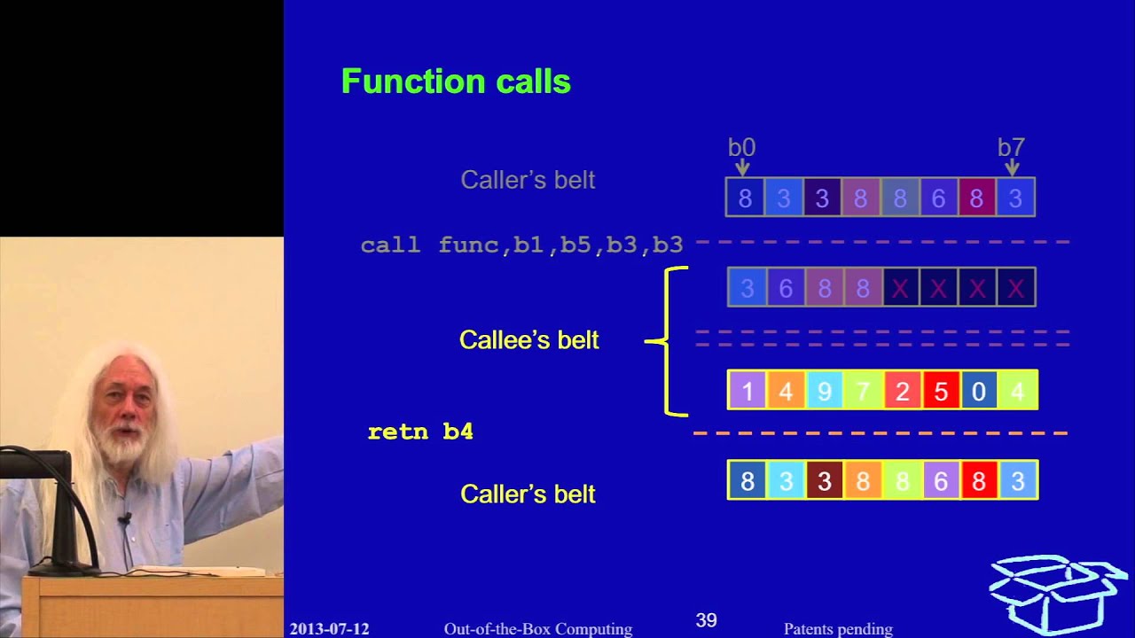
Calling a function on the Mill requires no tedious register saving, reloading, or stack warm-up protocols. The caller simply issues a `call` operation specifying the target function and the belt positions of the arguments. One cycle later, execution enters the callee with an empty, fresh belt that is preloaded only with copies of the passed arguments.

When the callee finishes its work, it executes a `return` operation. Exactly one cycle later, the caller resumes with its belt completely untouched and intact, except that the callee's returned results are dropped right onto the front of the belt. Calls can return multiple values just as cleanly as single values, making a function call behave uniformly like an ordinary operation. As the speaker notes:

> “So, a call has the same effects as an operation like add. And a call can drop multiple results.”

Language features like Ada `out` parameters or C++ `std::pair`—constructs invented to work around the linear, left-to-right constraints of human programming languages that obscure true dataflow graphs—are transformed directly by the toolchain into clean, multi-result functions.

- Function calls require zero prologue/epilogue register saving or restoring instructions. - Caller arguments are copied directly into the callee's brand-new belt. - Callee returns drop single or multiple values directly onto the restored caller belt in a single cycle.

[30:46](https://www.youtube.com/watch?v=QGw-cy0ylCc&t=1846s) Belt Save/Restore and the Spiller

The seamless reappearance of the caller's belt after a function returns is managed automatically by a dedicated background hardware engine called the spiller. Similar in purpose to SPARC register windows or Intel Itanium register stack engines, the spiller operates entirely behind the programmer's back without requiring explicit save/restore instructions.

Every value residing on the belt is tagged with a hardware frame ID (for example, frame 742) in addition to its positional belt index. A running function can only reference values whose frame tag matches the current execution frame ID. Switching frames on a call instantly hides the old values, leaving the new function with an empty belt, while the physical data remains stored in background buffers to be saved and restored by the spiller at leisure. Because arguments are passed by copy, they are stamped with the callee’s new frame ID; the caller cannot touch them during the call, and the callee cannot see the caller's older values.

[32:28](https://www.youtube.com/watch?v=QGw-cy0ylCc&t=1948s) Functional Unit Pipelines and Mux Sources

Functional units such as ALUs and shifters are grouped into clusters, slots, or pipelines that share common input wiring. Each pipeline on the Mill has exactly two data inputs shared across all internal units, while output connections are separated by operation latency. A single-cycle `add` routes out through latency-one outputs, whereas a three-cycle `mul` routes through latency-three outputs.

Each latency output feeds an internal, non-addressable capture register. Because operations like divide can produce multiple outputs per latency, every capture register constitutes an internal source that can be routed back as an input to other functional units. Encoding constraints dictate that the total number of physical sources must be at least twice the belt length. On the large "Gold" configuration of the Mill, the native outputs do not quite reach that threshold, so additional buffering is added to bring the machine to 64 total sources—an astonishingly small number when compared to the roughly 450 sources typical of an out-of-order superscalar design. As the speaker emphasizes:

> “This is the major reason why we are showing DSP power rather than superscalar power consumption.”

| Architecture Metric | Typical Superscalar | Mill "Gold" | |:--- |:--- |:--- | | **Bypass / Operand Sources** | ~450 sources | 64 sources | | **Power Profile** | High superscalar dissipation | Low DSP-level dissipation | | **Pipeline Input Ports** | Dynamic rename crossbars | 2 shared inputs per pipeline |

[35:00](https://www.youtube.com/watch?v=QGw-cy0ylCc&t=2100s) Wide Issue and Exposed Pipeline Execution

The Mill uses a wide-issue, statically scheduled model reminiscent of VLIW or Itanium. A single instruction word contains multiple operations packed into slots, which are issued simultaneously to corresponding functional pipelines.

Because it is an exposed-pipeline architecture, operation latencies are directly visible to software rather than being hidden behind out-of-order scheduling hardware:

> “What that means is that the latency of operations is visible to the program.”

If an operation takes three cycles, its result simply will not appear on the belt until three cycles later. For an expression like `(A + B) - (C * D)`, an adder and a multiplier can issue in parallel in cycle one. If the add completes in one cycle while the multiply requires three, the add result could sit on the belt waiting for the multiply, but letting idle results occupy belt positions wastes slots. Instead, code schedules best when producers feed directly into consumers: starting the multiply first, starting the add two cycles later, and issuing the subtract precisely when both results emerge together. This leaves the adder slot open during earlier cycles to perform unrelated work for other operations.

```mermaid flowchart TD accTitle: Producer-to-Consumer Scheduling accDescr: Scheduling multi-cycle multiply before single-cycle add so both complete simultaneously for subtraction. subgraph Cycle0["Cycle 0"] Mul["Multiply (Latency: 3 Cycles)"] end subgraph Cycle1["Cycle 1"] Other["Other Work (Adder Slot Free)"] end subgraph Cycle2["Cycle 2"] Add["Add (Latency: 1 Cycle)"] end subgraph Cycle3["Cycle 3"] Sub["Subtract (Consumes Add and Mul Results)"] end Mul --> Sub Add --> Sub ```

[38:43](https://www.youtube.com/watch?v=QGw-cy0ylCc&t=2323s) In-Flight Operations Across Calls

An exposed pipeline raises a subtle design question: what happens if a multi-cycle operation is in flight when a function call occurs? If code issues a signed integer multiply (`mulS`) and immediately calls another function on the next cycle, the multiply's result will become ready while execution is inside the callee.

The hardware does not drop the caller's multiply result into the middle of the callee's belt. Instead, the operation remains bound to the frame in which it was issued. The callee executes to completion, returns, and restores the caller's belt frame. Only then does the in-flight multiply retire into the caller's restored frame:

> “So, the multiply retires in the frame in which it was issued. Intervening calls are like intervening adds. Nothing happened.”

[40:26](https://www.youtube.com/watch?v=QGw-cy0ylCc&t=2426s) Interrupts as Involuntary Function Calls

An audience member interrupts with a critical question regarding in-flight operations over a function call: where does an in-flight operation's result go in the meantime? The questioner points out that it cannot remain stuck in the multiplier, or else the system would be ruined. The speaker reassures the audience that the answer is coming right up, explaining that fundamentally the mechanism relies on a hardware component called the "spiller."

Calls on the Mill architecture are atomic, and in-flight operations retire after the called function returns. This exact mechanism provides an elegant, unified way to handle hardware interrupts. On conventional processors, an interrupt requires complex context switching, dedicated shadow registers, or pipeline flushing. On the Mill, an interrupt is handled identically to a normal function call. As the speaker explains:

> “And is on a Mill nothing but a spontaneous function call that you didn't have to code.”

They are simply involuntary function calls. The processor hardware automatically vectors execution to the interrupt service routine's entry point and supplies the interrupt arguments directly onto the handler's belt. Because this follows standard call semantics, there is no duplicated hardware state (such as separate register banks for application and interrupt contexts), no task switch overhead, and no need to flush the pipeline. When the handler completes and returns, execution resumes without any restart penalty.

The only penalty incurred during an interrupt stems from branch prediction. Because the instruction decoder was busily decoding along the application's instruction stream and was not expecting the interruption, the arrival of an interrupt registers as a misprediction. On the Mill, an instruction mispredict costs only four clock cycles plus the top-level cache access time, and that is the entirety of the interrupt delay.

- Interrupts are treated identically to hardware-initiated function calls with arguments deposited directly onto the handler's belt. - No duplicate register sets for supervisor or interrupt modes are required. - No pipeline flushes or task-switch overhead occur on interrupt entry or exit. - Mispredict recovery cost on the Mill is strictly four cycles plus top-level cache access time.

---

[42:17](https://www.youtube.com/watch?v=QGw-cy0ylCc&t=2537s) Data Forwarding via a Two-Stage Crossbar

The belt is not implemented in silicon as an enormous, power-hungry shift register. Moving massive quantities of bits physically across silicon on every clock tick would be prohibitively expensive. Instead, internal data forwarding is handled by a two-stage crossbar interconnect. While software engineers often treat physical implementations conceptually, leaving specific multiplexer tree topologies to hardware designers, the underlying hardware model relies on segregating operations by latency.

Results produced by single-cycle operations—such as basic integer adds, shifts, and bitwise logical operations—must reach their consumers immediately to sustain tight back-to-back operational dependencies. To achieve single-cycle throughput without stalling, the Mill features a dedicated single-cycle crossbar linking all single-cycle producers (primarily the ALUs) directly to all potential consumers. This single-cycle path incurs a delay of only one or two multiplexer levels.

Longer-latency units—such as floating-point units and byte/vector shufflers—route through a separate latency-$N$ crossbar. This crossbar narrows down the broad array of multi-cycle operational outputs into two inputs, which are then fed into the latency-1 crossbar to reach execution consumers.

```mermaid flowchart TD accTitle: Two-Stage Crossbar Data Forwarding accDescr: Diagram showing how single-cycle ALU operations feed directly to consumers while multi-cycle units funnel through a latency-N crossbar first.

subgraph Producers ["Execution Units"] ALU["Single-Cycle ALUs<br/>(Adds, Shifts, Bitwise)"] Multi["Multi-Cycle Units<br/>(FPUs, Shufflers, Multipliers)"] end

subgraph Crossbars ["Interconnect Network"] LatN["Latency-N Crossbar<br/>(Windows down to 2 outputs)"] Lat1["Latency-1 Crossbar<br/>(1-2 mux levels)"] end

Consumers["Execution Unit Consumers"]

Multi --> LatN LatN --> Lat1 ALU --> Lat1 Lat1 --> Consumers ```

- System clock timing is defined by the duration of a 32-bit addition plus the traversal through the latency-1 crossbar. - The single-cycle crossbar introduces only one to two levels of mux latency depending on the number of ALUs. - Multi-cycle operations span several internal clock boundaries and borrow a portion of the trailing cycle slack because the latency-$N$ crossbar does not require an entire cycle.

---

[45:31](https://www.youtube.com/watch?v=QGw-cy0ylCc&t=2731s) Retiring Operations of Differing Latencies

The Mill instruction encoding specifies exactly one operation per pipeline issue slot per clock cycle. Once issued into a pipeline, an operation matures internally within its functional unit and retires onto the belt an exact number of cycles later matching its specific latency.

To illustrate how varying latencies interact, the speaker traces a sequence issued into a single pipeline across sequential clock cycles: 1. **Cycle 0:** A binary floating-point add (`addB`), which has a 4-cycle latency, issues. Its intermediate state begins advancing through the floating-point pipeline. 2. **Cycle 1:** A signed integer multiply (`mul`), a 3-cycle operation, issues into the integer multiplier unit while the floating-point add continues processing. 3. **Cycle 2:** A vector widening operation (`widenM`), which takes a vector of shorts, converts it into two vectors of 32-bit words, and has a 2-cycle latency, issues into its functional unit. 4. **Cycle 3:** A standard unsigned integer add (`add`), a 1-cycle latency operation, issues into the ALU.

Because each successive operation had a latency exactly one cycle shorter than the operation issued before it, all four operations complete at the very same instant. On Cycle 4, every one of these operations retires to the belt simultaneously.

- Each functional unit maintains its own internal pipeline stages, allowing different units within the same pipeline to advance simultaneously. - Multiple operations issued across consecutive cycles can retire together in the exact same cycle if their latency countdowns align. - An operation can produce multiple retirement outputs simultaneously, such as `widenM` producing two distinct result vectors.

---

[48:13](https://www.youtube.com/watch?v=QGw-cy0ylCc&t=2893s) Output Registers, Daisy-Chaining, and the Spiller

Every functional pipeline contains output registers designated by latency (`lat1`, `lat2`, `lat3`, `lat4`). If an instruction stream executes repeated single-cycle adds back-to-back, the first add moves into the `lat1` register after one cycle. When the next add completes, `lat1` is occupied. However, the `lat2` register is guaranteed to be vacant because the only way `lat2` could contain a value is if a 2-cycle operation had been issued a cycle earlier—which the program did not do.

Consequently, results daisy-chain upward across the latency registers without hazard or collision: the existing value steps up from `lat1` to `lat2`, and the newest result enters `lat1`. This progression continues along the chain as more adds execute. When values must be preserved, hardware only needs to extract data spilling off the end of the highest-latency register (`lat4`).

When the latency registers become entirely saturated, the processor routes the overflowing value off `lat4`. The data may be directed to a vacant register in another pipeline or moved into a dedicated bank of buffer registers managed by the spiller. This answers the audience's earlier question about where values live over function calls: an in-flight multiply that matures over a call shifts down the daisy-chain into the spiller's buffer registers. The spiller moves these values into fast internal SRAM, and, if the call chain runs deep enough, out into DRAM and the broader memory hierarchy, eventually replaying them back into top-level registers upon return.

Hardware implementations can vary—utilizing a register file, implementing the belt as a Content-Addressable Memory (CAM), or applying other circuit topologies—provided there are sufficient latency and buffer registers to match belt positions. Software remains completely agnostic to these physical trade-offs.

---

[52:16](https://www.youtube.com/watch?v=QGw-cy0ylCc&t=3136s) Architectural Summary: The In-Order, Exposed Pipeline

The speaker summarizes the core architectural principles that differentiate the Mill from traditional out-of-order processors. The Mill operates strictly in-order: instructions execute in program order, and execution scheduling is handled statically by the compiler rather than dynamically by silicon schedulers. Because the compiler controls issue timing and pipeline latencies are fully exposed, the compiler knows the exact cycle in which every result retires.

General-purpose architectural registers are completely eliminated; transient values live entirely on the temporary belt. Because every belt position adheres strictly to Static Single Assignment (SSA) form, values are immutable and cannot introduce write-after-read (WAR) or write-after-write (WAW) hazards. As a direct consequence, register renaming is completely unnecessary.

Without the overhead of complex hardware renaming, dynamic issue scheduling, and out-of-order retirement, the Mill pipeline is remarkably compact:

> “The Mill has only four, which means that a mispredict is a third of the cost of a mispredict on a different machine.”

While modern superscalar microarchitectures like Intel Haswell feature deep stacks of pipeline stages (and historical designs like Pentium 4 NetBurst reached over thirty stages), the Mill requires only four pipeline stages. Furthermore, because result destinations are implicitly assigned to the front of the belt, instructions omit explicit destination addresses, resulting in dense, compact binary code.

| Architectural Feature | Conventional Modern Out-of-Order (e.g., Haswell) | Mill CPU Architecture | |:--- |:--- |:--- | | **Execution Ordering** | Dynamic, out-of-order hardware scheduling | Static, in-order compiler scheduling | | **Pipeline Latency** | Hidden / dynamic | Fully exposed to the compiler | | **Intermediate Storage** | Named general-purpose register files | Implicit FIFO-like temporal belt | | **Hazard Resolution** | Dynamic register renaming hardware | SSA representation on belt (no renaming) | | **Pipeline Depth** | Deep (14–20+ stages; 30+ on NetBurst) | 4 stages | | **Branch Mispredict Penalty** | High (typically 14–20+ cycles) | 4 cycles plus top-level cache access time | | **Result Addressing** | Explicit destination register encoded in instruction | Implicit push to the head of the belt |

[53:46](https://www.youtube.com/watch?v=QGw-cy0ylCc&t=3226s) Function Calls, Argument Passing, and Upcoming Talks

Because the Mill architecture eliminates register specifiers in favor of temporal belt positions, instruction encodings remain exceptionally compact, saving substantial silicon footprint, wire routing, and power within the instruction cache. The architecture naturally handles multi-result operations without awkward register-pairing workarounds. Furthermore, function calls and returns take only a single cycle and a single operation, eliminating the traditional compiler-generated prelude and postlude entirely. Callers can pass up to an entire belt's worth of arguments directly. If a routine requires more parameters than fit on the belt, or if it passes massive structs or variable argument lists (`varargs`), those spill over into memory just as they do on conventional platforms. For the vast majority of software, however, parameters remain entirely on the belt. As Ivan Goddard puts it:

> “Anything you could pass to the registers you can pass to the belt.”

Additional technical resources, white papers, and recorded presentations are hosted on the project website. The team maintains a strictly technical mailing list focused on publishing notifications for upcoming white papers and appearances. Scheduled presentations include upcoming sessions with the IEEE, two presentations at Stanford University, and a planned event at Microsoft, with each talk exploring distinct facets of the architecture. Goddard notes that the immediately following talk will examine the memory hierarchy, detailing how the Mill avoids pipeline stalls—a challenge that historically hobbles statically scheduled machines.

- Calls and returns execute in a single cycle and a single instruction with zero prelude or postlude code. - Argument passing supports up to a full belt capacity; oversized structs and `varargs` fall back to standard memory passing. - Upcoming technical presentations announced for IEEE, Stanford, and Microsoft, including an in-depth session on memory hierarchy design.

---

[55:56](https://www.youtube.com/watch?v=QGw-cy0ylCc&t=3356s) Task Switching, OS Protection, and Multithreading vs. Multicore

When asked how the architecture coordinates thread scheduling, process contexts, and operating system state saves, Goddard clarifies that raw hardware has no intrinsic concept of an operating system. The Mill is engineered as a general-purpose processor capable of hosting standard operating systems like Linux and Windows. Task switches function under the exact same mechanics as standard function calls: the operating system executes a call into a context-switch routine, which subsequently returns into the target thread, leaving the hardware spiller to transparently save and restore the underlying belt state.

Addressing security and isolation, Goddard previews the Mill’s unique protection architecture. Rather than relying on hardware protection rings, supervisor modes, or privileged instructions, all system protection is enforced directly through the memory addressing environment:

> “The Mill does not have rings. It has no supervisor mode. There are no privileged operations. All protection is done through the memory addressing environment.”

On the subject of hardware multithreading, Goddard reveals that current Mill chips intentionally omit simultaneous multithreading (SMT). Extensive architectural simulations demonstrated that dedicating chip area and electrical power to additional physical cores yields vastly superior performance compared to multiplexing multiple threads onto a single core. Conventional superscalar designs implement multithreading primarily to keep execution units occupied during high-latency L2 cache misses. Because the Mill’s architecture fundamentally experiences far fewer cache misses and incorporates alternative stall-hiding mechanisms, it avoids the memory latency bottlenecks typical of conventional processors. Goddard notes that while random lookups across massive hash tables exceeding cache size will inevitably run at raw memory speeds on any architecture, the Mill hides typical latencies without the structural baggage of SMT.

```mermaid flowchart TD accTitle: Mill Protection and Thread Model accDescr: Diagram illustrating how the Mill processor relies on memory addressing for protection and favors multicore scaling over hardware multithreading.

subgraph ProtectionModel["Protection Model"] direction TB P1["Uniform Execution Mode"] --> P2["No Rings / No Supervisor Bit"] P2 --> P3["Memory Addressing Capability Enforces Security"] end

subgraph CoreStrategy["Core Allocation Strategy"] direction TB C1["Avoid SMT / Hyperthreading"] --> C2["Eliminate Thread-Switching Overhead"] C2 --> C3["Dedicate Die Area & Power to Multiple Physical Cores"] end ```

- Hardware has no supervisor rings or privileged opcodes; access control is mediated entirely by whether software possesses a valid, usable address. - Simultaneous multithreading is omitted; hardware simulations proved that silicon area and power budgets deliver higher throughput when allocated to additional cores. - SMT on out-of-order chips exists primarily to hide L2 cache miss penalties, which the Mill mitigates through internal pipeline and memory designs.

---

[01:00:39](https://www.youtube.com/watch?v=QGw-cy0ylCc&t=3639s) Hardware Implementation: Pipeline Latencies and Associative Belt Tagging

An audience member asks for clarification regarding the relationship between functional pipeline latency stages (latencies one through four) and specific belt positions, inquiring whether the machine relies on an out-of-order core, CAM lookups, or centralized crossbar routing. Goddard emphasizes that the belt is not a monolithic physical shift register, register file, or SRAM block. Instead, discrete pipeline output registers hold values that are explicitly tagged with a frame ID, producing operation ID, and current belt position. When an instruction requests an operand, the consumer functional unit broadcasts a request for a specific frame and belt offset, prompting the matching physical register to provide the data. Belt advancement is accomplished simply by broadcasting an offset update across the tagged registers:

> “The way we advance the belt is we tell all of those registers, ‘Add two to your belt number.’ It’s that easy.”

Addressing crossbar interconnects, Goddard explains that the pipeline employs two daisy-chained crossbars. Time-critical single-cycle operations utilize only the primary latency-one crossbar to meet aggressive clock targets, whereas multi-cycle operations traverse both crossbars in succession. Hardware implementers can realize operand routing in several ways: designers can either implement content-addressable memory (CAM) where matching registers self-identify, or use decode and issue logic to track operand locations statically and drive crossbar multiplexers directly.

```mermaid flowchart LR accTitle: Belt Operand Resolution accDescr: Flow diagram showing how consumer instructions match tagged registers or route through crossbars to obtain operands.

subgraph BeltState["Tagged Registers"] R1["Register A<br/>Frame: 742 | Belt: B3"] R2["Register B<br/>Frame: 742 | Belt: B1"] end

subgraph Query["Consumer Request"] C["Consumer Op<br/>Needs Frame 742, B3"] end

subgraph Interconnect["Routing"] X1["Latency 1 Crossbar<br/>(Clock Critical)"] X2["Latency 2+ Crossbar<br/>(Chained)"] end

C -.->|"Broadcast Target"| R1 R1 -->|"Match Found"| X1 X2 --> X1 ```

- Belt storage does not use a central register file; values sit in pipeline output registers tagged with frame ID, generating operation, and belt index. - Advancing the belt does not shift data physically; the controller commands active registers to increment their belt index tags. - Routing utilizes two daisy-chained crossbars, isolating latency-one operations onto a high-speed routing stage to prevent clock cycle degradation. - Operand matching can be implemented either associatively via CAMs or deterministically via instruction decode tracking logic.

---

[01:02:58](https://www.youtube.com/watch?v=QGw-cy0ylCc&t=3778s) Crossbar Contention and Multi-Consumer Data Distribution

In response to questions regarding whether inputs ever compete over crossbar sinks or experience dynamic congestion, Goddard states that input routing is completely deterministic. Each execution pipeline requires two operand inputs, and the compiled instruction bundle specifies the exact belt locations feeding those inputs. Because input requirements are scheduled in advance, structural collisions cannot occur at the sink. Multiple functional units can freely read from the exact same belt location in the same cycle without conflict, mirroring how multiple ALUs in an out-of-order machine can read the same physical source register.

Managing outputs requires ensuring that multi-cycle results do not overwrite older values that must remain accessible to subsequent operations. Goddard explains that pipeline stages move results along daisy-chained intermediate registers within functional pipelines until they reach their final retirement latency, after which they migrate into staging buffers. When asked if the architecture relies on multi-ported SRAM—particularly for managing wide execution configurations where 30 parallel operations might simultaneously read from a single belt position (creating up to 60 concurrent reads)—Goddard clarifies that the core avoids complex multi-ported SRAM arrays. Instead, broadcast values drive functional units directly from flip-flop registers, while the background memory spiller relies on standard single-ported SRAM banks. Goddard highlights the extreme fan-out requirement handled by the design:

> “It is required that a single belt position be able to feed data to every possible consumer of of a particular cycle.”

- Instruction streams explicitly dictate operand origins, preventing input port collisions and eliminating runtime routing contention. - A wide 30-wide instruction packet with two inputs per operation represents up to 60 concurrent operand reads from the belt in a single clock cycle. - Extreme fan-out scenarios (all units reading the same belt position) are sourced directly from dedicated flip-flop register outputs rather than heavily ported SRAM arrays. - Backing buffers and spiller hardware rely on efficient, single-ported SRAM structures rather than costly multi-ported storage.

[01:05:45](https://www.youtube.com/watch?v=QGw-cy0ylCc&t=3945s) Compiler Simplicity and Time-Reversed Scheduling

An audience member asks what a compiler targeting the Mill architecture must optimize compared to compilers targeting conventional superscalar processors. Ivan Godard answers from the perspective of an industry veteran who has written nearly a dozen compilers over his career. He notes that chip architects often pass the buck by claiming the compiler will work out all the difficult hardware complexities, leaving the hardest optimization problems as an afterthought. Determining to avoid that trap, the Mill team designed the machine to be fundamentally "compiler-easy," stripping away the need for exotic target-specific heuristics. Beyond standard machine-independent optimizations like constant folding—which Mill is handling by integrating with LLVM—the backend pipeline requires very little optimization.

When generating code specifically for the belt, the compiler's primary job is simply scheduling producers so that their retiring outputs align directly with when downstream consumers need them. Ivan explains that the Mill achieves this by borrowing a proven 40-year-old technique widely used in signal processing compilers: scheduling in reverse time order. The compiler examines the final consumer—such as a function return—schedules it, and then steps backward along the dataflow graph, scheduling each preceding producer according to its pipeline latency. Because the hardware offers a single, predictable way to execute each operation rather than a tangled web of specialized processor states, the compiler does not need complex case-selection logic.

“I've had much bitter experience of people who design chips and say, 'Well, the magic's in the compiler.' And they push that off until the last,” Ivan remarks, drawing knowing chuckles from compiler engineers in the room.

```mermaid flowchart TD accTitle: Time-Reversed Instruction Scheduling accDescr: Dataflow pipeline scheduled in reverse order from terminal consumer back to producers. subgraph Sched ["Reverse Time Scheduling"] direction TB Ret["1. Schedule Terminal Consumer (e.g. Return)"] Pred1["2. Step Back Latency Cycles: Schedule Immediate Producer"] Pred2["3. Step Back Latency Cycles: Schedule Source Operands"] Ret --> Pred1 Pred1 --> Pred2 end ```

[01:08:41](https://www.youtube.com/watch?v=QGw-cy0ylCc&t=4121s) Simulator Status, Toolchain Maturity, and Startup Constraints

Responding to an audience question about the public availability of the Mill compiler and architectural simulator, Ivan provides a frank assessment of where the project stands. While the architecture has been running inside an internal software simulator for several years, the surrounding toolchain remains what he politely calls "alpha grade." As a small, self-funded bootstrap startup, Mill Computing has focused strictly on the novel architectural components necessary to validate the design. Major functional blocks that are standard industry commodities—such as standard IEEE floating-point units—have not even been built internally because the company plans to license proven third-party IP rather than reinvent existing technology.

Public distribution of the simulator and tools is currently blocked by resource constraints, as supporting general public users would overwhelm their small engineering team. However, Ivan indicates that the company is open to making arrangements with qualified, self-supporting individuals or organizations who can sign non-disclosure agreements, with the caveat that any intellectual property developed around the architecture must belong to Mill Computing.

“In order to let the public play with it, we would have to be able to support the public,” Ivan admits. “And we haven't got the resources.”

- The Mill simulator has been actively running internal workloads for several years. - The software toolchain is operational for core validation but remains in an early alpha state. - Floating-point and other commodity logic blocks will be acquired as third-party IP rather than designed in-house. - Access is restricted to self-supporting partners under NDAs while the team seeks funding to expand support capabilities.

[01:10:28](https://www.youtube.com/watch?v=QGw-cy0ylCc&t=4228s) Belt Operand Uniformity: Vectors, Scalars, and Unified Types

An attendee asks whether supporting short vectors implies that individual slots on the belt can hold different operand widths, and whether differing widths restrict which functional units or instructions can consume them. Ivan confirms that each belt position is completely width- and type-agnostic. A slot can hold a single byte, a double word, a quad word, or a packed vector of half-words; every slot simply holds an operand.

Conventional processor architectures typically segregate values into distinct physical register files—such as separate register banks for integer, scalar floating-point, and SIMD/vector operations—primarily to reduce the excessive wire and port count of a massive unified register file. Ivan points out that partitioning register files introduces immense friction into compilers and hardware alike, forcing costly and awkward cross-bank moves whenever code performs operations like converting a floating-point number into an integer. The Mill avoids this entire class of problems by allowing any belt instruction to consume any operand slot regardless of its underlying format.

“The belt holds an operand, any kind of operand the machine supports,” Ivan emphasizes.

[01:11:50](https://www.youtube.com/watch?v=QGw-cy0ylCc&t=4310s) Variable Latency, Cache Misses, and Memory Timing

When asked how an in-order machine with a belt handles variable-latency operations—such as data cache hits versus misses—Ivan notes that while the exact internal mechanics of the memory hierarchy are reserved for an upcoming talk pending patent filings, he can explain the programming model's guarantees. Despite executing strictly in-order without the massive hardware reorder buffers found in out-of-order processors, the Mill architecture successfully hides the operational latency of L1 and L2 caches completely.

Furthermore, Ivan explains that the Mill can hide main DRAM latency in the exact same application profiles where an out-of-order superscalar processor could hide it. An audience member asks if this means the machine stalls on memory delays, but Ivan flatly rejects that characterization. While neither an out-of-order core nor the Mill can hide memory latency during truly unpredictable memory traversals—such as pointer chasing or random accesses across a hash table—the Mill matches out-of-order tolerance for predictable patterns while completely eliminating out-of-order hardware overhead.

“We succeed in hiding the latency of both levels of cache and can hide the latency of DRAM in those cases in which an out-of-order machine could hide the latency of DRAM,” Ivan asserts.

[01:13:47](https://www.youtube.com/watch?v=QGw-cy0ylCc&t=4427s) Patent Law Changes, Stealth Mode, and the Disclosure Schedule

Asked when Mill Computing will publish an official instruction set manual, Ivan explains that publishing the raw instruction set would prematurely disclose proprietary mechanisms whose patents are still in flight. He recounts how the company operated in complete stealth mode until September 2012, when changes to United States patent law—specifically the transition from a "first-to-invent" to a "first-to-file" system under the America Invents Act—forced an abrupt pivot. The shift made prolonged secrecy dangerous, prompting the team to rapidly write and submit over fifty distinct patent applications.

Ivan vents about the grueling effort required to document these innovations legally while simultaneously preparing deep-dive technical talks, noting that the team aims to unveil a new functional area of the machine approximately once a month. When another audience member asks if memory loads require a dedicated spill buffer to manage asynchronous arrival times, Ivan clarifies that loads behave just like any other functional operation: their results drop straight into the front of the belt, and their arrival timing is fully known and deterministically coordinated.

“With the change from first to invent to first to file, we were in a situation where, guys, we can't keep on being in stealth mode,” Ivan explains. “We are going to have to file these and now.”

- Over fifty patents have been drafted and filed by the Mill Computing team. - Public technical presentations began after an initial presentation at the USENIX conference in Vail, Colorado in June 2013. - Memory loads drop directly into the front belt position (slot 0) on arrival, behaving identically to computational functional unit results.

[01:16:05](https://www.youtube.com/watch?v=QGw-cy0ylCc&t=4565s) Binary Compatibility Across Processor Families: The AS/400 Approach

The session concludes with an audience member addressing the trade-offs of static scheduling across a diverse hardware family. If different Mill models feature varying belt capacities, pipeline depths, and functional unit counts, does every model require a completely different, recompiled binary? Ivan explains that the Mill solves this problem using the battle-tested deployment model pioneered by IBM for the System/38 and AS/400 lines, which has preserved software compatibility across four decades of radical hardware evolution.

Instead of shipping low-level hardware bit patterns directly to users, Mill software is distributed in an abstract, platform-independent intermediate representation. When a software package is installed onto a specific target device, an install-time specialization tool translates the abstract representation into the native machine code optimized for that exact processor configuration—its specific belt length, functional unit count, and execution latencies. Consequently, different chips within the Mill family remain entirely incompatible at the raw machine-instruction bit level, yet retain complete application-level portability across the entire ecosystem.

“Consequently, the individual family members at the bit level are incompatible in terms of their instructions,” Ivan explains, emphasizing that portability lives in the intermediate representation rather than an immutable legacy machine code.

[01:17:02](https://www.youtube.com/watch?v=QGw-cy0ylCc&t=4622s) Target Workloads, Peak vs. Sustained IPC, and the Gold Configuration

An audience member asks about expected performance: with 33 functional units operating in parallel, what kind of effective instruction count or instructions per cycle (IPC) does the architecture achieve across different application types? The speaker clarifies that the "Gold" configuration shown in the presentation is not designed to be an HPC (high-performance computing) chip. Instead, Gold targets general-purpose server workloads—the kind of compute infrastructure Google runs in its data centers. Because of this target, Gold offers numerous operation slots to exploit parallelism, but its vector width is modest; it includes only two floating-point units. By contrast, a high-performance compute variant intended for scientific institutions like NASA would provide eight floating-point units and process 128 bytes at a time. Performance characteristics will therefore vary substantially across different members of the Mill family depending on hardware specialization.

```mermaid flowchart LR accTitle: Mill Family Configuration Comparison accDescr: Comparing the Mill Gold server chip with an HPC chip variant. subgraph Gold["Mill Gold (Server Target)"] G1["Target: Web & Enterprise Servers"] G2["High slot count (33-issue peak)"] G3["2 Floating-Point Units"] G4["Moderate vector width"] end subgraph HPC["HPC Variant (Scientific/NASA)"] H1["Target: High-Performance Computing"] H2["8 Floating-Point Units"] H3["128-byte vector paths"] end ```

When pressed on typical server benchmarks like SPEC CPU, the speaker points out that discussing performance outside actual customer code runs often comes down to peak numbers. “That Gold can issue 33 operations per cycle sustained. But that is peak. That's not simulated performance. It can do this.” He emphasizes that hardware width delivers high performance only when the compiler can pipeline the loop bodies. If code has serial data dependencies where step B strictly requires step A, the Mill must execute operations one at a time, just like any conventional machine. “The width is intended for pipelining. Because 80% of code is pipelined.”

- **Mill Gold specification:** Server-oriented design with 33 operation slots peak issue per cycle and two FPUs. - **Mill HPC specification:** Scientific variant with eight FPUs and 128-byte vector paths. - **Serial code behavior:** Code with strict sequential dependencies falls back to executing single operations sequentially, meaning wide issue capability offers no benefit unless loops are pipelined.

---

[01:19:28](https://www.youtube.com/watch?v=QGw-cy0ylCc&t=4768s) Pipelining in Action: The Unix `wc` Optimization Example

To illustrate how software pipelining exploits the architecture's wide execution engine, the speaker references an assembly optimization contest centered around the classic Unix `wc` (word count) utility. Standard naive implementations of `wc` read an input character and dispatch it through a `switch` statement checking whether it is whitespace, a newline, or ordinary text. On modern pipelines, this approach incurs devastating branch mispredictions. On the Mill, the compiler transforms the sparse `switch` statement into a chain of `if` statements and then applies `if-conversion`. This converts conditional control flow directly into a data-flow graph using conditional operations (analogous to conditional moves on x86), eliminating internal branches entirely except for the single loop branch.

Once the control-flow branches are eliminated, all switch outcomes evaluate concurrently. For modern `wc` implementations—which track not just character, word, and line counts, but also the length of the longest line—the entire loop body compiles down to 25 operations. On the Gold chip, those 25 operations execute simultaneously in a single cycle. The Mill can therefore ingest and process one full character per cycle out of the input stream. This dramatic throughput is achieved purely through software pipelining and data-flow conversion mapped across the machine's functional units.

---

[01:22:43](https://www.youtube.com/watch?v=QGw-cy0ylCc&t=4963s) Absence of Condition Codes and Global Architectural State

When asked whether the Mill architecture features condition codes, the speaker responds with an emphatic negative. “The machine maintains no global state at all. No global application state like the condition codes have.” In traditional architectures, condition flags create hidden dependencies across instructions and complicate out-of-order execution, register renaming, and pipeline speculative state. On the Mill, comparison results and conditional operations do not set side-channel flags; instead, all comparison outputs produce standard values that are placed directly onto the belt as regular data items.

---

[01:23:18](https://www.youtube.com/watch?v=QGw-cy0ylCc&t=4998s) Stack Inspection, Garbage Collection, and the Spiller Debugging API

An attendee raises the challenge of runtime stack inspection for garbage collectors, language runtimes, and profilers. On conventional register architectures, inspecting stack frames and register state is well-understood, whereas hardware that hides activation state behind specialized mechanisms (such as register windows on SPARC) can incur severe runtime penalties when forcing that state into memory. The questioner asks if a garbage collector on the Mill must spill all belt state to main memory to perform a root scan.

```mermaid flowchart TD accTitle: Debugger and GC Stack Inspection Path accDescr: How debuggers and garbage collectors access state buffered in the hardware spiller. A["Active Frame on Belt"] --> B["Nested Function Call"] B --> C["Caller State Pushed to Hardware Spiller SRAM"] C --> D{"Debugger / GC Inspection Request"} D --> E["Spiller API Accesses Internal SRAM"] E --> F["State Flushed to Memory Lazily / on Demand"] F --> G["Garbage Collector Scans Standard Memory"] ```

The speaker explains that conventional garbage collectors already implement special cases for CPU registers, and an engine on the Mill would similarly handle the belt. For deeper stack frames beneath the current function, state is managed automatically by the hardware spiller. When deep nested calls are made, parent frames migrate into the spiller's internal SRAM. The Mill provides a dedicated hardware access mechanism and an API specifically designed for debuggers to walk and inspect non-top frames:

- **Debugger/GC API:** Exposes hardware hooks to read frame data directly from the spiller. - **Cost:** Inspecting frames through this API merely requires accessing memory. - **Flushing Behavior:** While accessing the API forces the spiller's internal SRAM to flush, that flush normally occurs lazily through the regular overhead of invoking the debugging or profiling infrastructure itself. - **SPARC comparison:** The attendee observes that on SPARC, window flushing makes GC activation significantly slower than on flat register files, but the speaker confirms that once the spiller memory is addressed, memory scanning proceeds in standard linear memory without exotic penalties.

---

[01:25:57](https://www.youtube.com/watch?v=QGw-cy0ylCc&t=5157s) Concluding Remarks and Upcoming Presentations

Noting the time has passed 9:00 PM, the speaker checks whether the audience wants to continue or wrap up, joking that he would happily talk about his "baby" all night. Seeing the signal from event organizers to conclude, he closes the session and thanks the audience for attending.

During the sign-off, an attendee asks about the location of the upcoming memory subsystem talk and whether it will take place at Stanford. The speaker clarifies that their next Stanford appearances are scheduled for October and February. For details on upcoming talks and locations outside Stanford, he directs attendees to sign up for the company's mailing list on the Mill Computing website.

## Notable quotes > [55:56](https://www.youtube.com/watch?v=QGw-cy0ylCc&t=3356s) The Mill does not have rings. It has no supervisor mode. There are no privileged operations. All protection is done through the memory addressing environment. — Ivan Godard

> [03:12](https://www.youtube.com/watch?v=QGw-cy0ylCc&t=192s) Signal processing is just not the same as general purpose code. — Ivan Godard

## Mentioned America Invents Act, AS/400, Google, IBM, IBM System/360, IEEE, Intel Haswell, Intel Itanium, Ivan Godard, Linux, LLVM, Microsoft, Mill Computing, Inc., Mill Gold, NASA, Pentium 4 NetBurst, SPARC, SPEC CPU, Stanford University, System/38, Unix wc, USENIX, Windows, Yale Patt

## Video description Please share via this link: http://MillComputing.com/docs/belt/

00:00:00  01   The Belt - a new machine model 00:00:37  02   Two architectures 00:03:12  05   Why huge cost in both power and price? 00:04:31  06   Our result - rough numbers 00:06:33  09   33 MIMD operations per cycle peak 00:07:24  10   33 operations per cycle peak ??? Why? 00:09:59  11   33 operations per cycle peak ??? How? 00:11:20  13   The problem - lots of producers and consumers 00:13:05  17   The cost - and performance limit 00:15:34  23   Why renames? 00:18:28  26   What are the temps used for? 00:19:12  27   Split the uses 00:20:33  29   What you really want... 00:20:55  30   We call it the Belt - like a conveyer belt 00:21:50  32   Multiple operation issue 00:21:58  33   Multiple operation retire 00:22:12  34   Belt addressing - temporal addressing 00:23:56  36   Use it or lose it 00:25:18  37   The scratchpad 00:27:12  38   Single operation with multiple results 00:28:24  39   Function calls 00:30:46  40   Belt save/restore 00:33:36  42   Functional unit pipelines - 64 sources vs 450 00:35:00  43   Wide issue 00:35:48  44   Exposed pipeline 00:38:43  47   In-flight over call 00:40:40  49   Interrupts, traps and faults 00:42:16  50   Data forwarding 00:44:31  51   Belt timing 00:45:30  52   Retiring ops of different latencies 00:48:12  54   Belt data location 00:52:16  57   Summary 00:54:32  60   Want more? 00:55:55               Questions 01:26:22               end 01:26:49               fin

[Source](https://www.youtube.com/watch?v=QGw-cy0ylCc)

中文简报

Mill摒弃寄存器改用传送带架构以降低处理器功耗 以时序传送带取代传统寄存器堆,消除了重命名硬件并大幅缩减旁路多路复用器源,在数字信号处理器级别的能效下实现每周期33次操作。 Ivan Godard介绍了Mill CPU架构及其核心机制Belt。Belt用时序FIFO结构取代了传统的通用寄存器,功能单元的输出从前端存入并随时间从后端移出淘汰。他阐述了标准的乱序超标量处理器如何将超过90%的功耗和芯片面积浪费在寄存器重命名以及用于处理临时数据的庞大旁路多路复用器树上。通过将执行延迟直接暴露给编译器并利用时序寻址,Mill消除了读后写和写后写冲突,省去了指令目标编码,并在DSP级别的能效下实现每周期高达33次MIMD操作。 Mill Computing推出了Belt,这是一种替代CPU操作数模型,用时序FIFO队列取代了传统寄存器堆和动态寄存器重命名。 (20:55) 通过从空间寄存器转向时序寻址,Mill核心将布线源从约450个削减至64个,大幅降低了占现代超标量处理器近半功耗的互连功耗开销。 (32:28) 旗舰级Mill Gold配置的目标是在1.2 GHz和28 W下实现每周期33次MIMD操作,通过编译器驱动的显式流水线调度提供高达80 GOPS的峰值性能。 (3:12) 不同Mill微架构之间的软件兼容性是通过源自IBM AS/400的安装时特化模型实现的,而非依赖固定的指令位模式。 (76:05)

Detailed notes — zh

## Background 本内容由 Mill Computing, Inc. 于 2013 年 7 月 29 日发布在 YouTube 平台上,是关于 Mill CPU 架构系统讲座的第二讲。根据页面说明,本期内容围绕名为“Belt”(传送带)的全新机器模型展开,详细探讨了现代芯片在功耗与价格上的困境,以及 Mill 架构如何通过革新数据流动模型实现极高能效的指令吞吐。 ## TL;DR 主讲人 Ivan Godard 对比了现代乱序超标量 CPU 与顺序执行 VLIW DSP 在能耗与架构上的巨大鸿沟,指出超标量核心由于依赖复杂的重命名机制和庞大的多路选择器互连网络,导致数据分发消耗了近一半的芯片功耗。为此,Mill 架构彻底抛弃了通用寄存器与寄存器重命名,提出了一种先进先出的时间寻址传送带模型——Belt,使算术操作结果隐式落入队列前端,并辅以硬件 Scratchpad 暂存器。通过仅 64 个源端的两级交叉开关网络、多结果原生支持以及后台静默运行的 Spiller 溢出引擎,Mill 在完全静态调度和暴露流水线下实现了单周期峰值高达 33 条 MIMD 操作的超宽吞吐,并以极低开销完成了零开销函数调用与瞬时中断响应。 ## Atmosphere & style 整场讲座兼具资深芯片架构师的硬核工程严谨与极客式的风趣幽默,主讲人以自嘲“幻灯片产品”和调侃营销部门开场,迅速拉近了与 Google 现场工程师听众的距离。在白板式的清晰逻辑推导下,复杂的底层硬件瓶颈被剥丝抽茧般剖析得透彻生动,面对传统体系结构的痼疾时言辞犀利切中要害。问答环节则火花四溅,面对关于超线程、硬件交叉开关及缓存停顿等尖锐技术追问,主讲人从容且充满信心地拆解回应,整场演讲弥漫着一种打破半个世纪传统架构教条的雄心与底层创新的技术激情。 ## Bulletin - [20:55](https://www.youtube.com/watch?v=QGw-cy0ylCc&t=1255s) Mill 架构摒弃了传统处理器的通用寄存器与寄存器重命名机制,提出先进先出定长队列心智模型的 Belt(传送带),通过时间相对寻址传递操作数,使机器指令无需显式编码结果地址。 - [04:15](https://www.youtube.com/watch?v=QGw-cy0ylCc&t=255s) 在能效与硬件规模上,主流乱序超标量 CPU 面对近 500 个数据源导致互连网络吃掉近半核心功耗,而 Mill 将数据源精简至 64 个,使双核 Gold 配置在 1.2 GHz 主频与 28 W 功耗下即可提供单核 33 ops/cycle 的峰值 MIMD 发射能力。 - [18:28](https://www.youtube.com/watch?v=QGw-cy0ylCc&t=1108s) 基于 Yale Patt 的统计,80% 的临时变量仅被消费一次,Mill 对其采用用完即从 Belt 尾端跌落的策略,剩余 14% 需要长效保留的值则通过固定 3 周期往返延迟的片上独立 Scratchpad 显式管理。 - [28:24](https://www.youtube.com/watch?v=QGw-cy0ylCc&t=1704s) 系统级交互全面简化:硬件采用 Frame ID 与后台 Spiller 引擎实现单周期无序言/结语的零开销函数调用与多返回值支持,外部中断被视作非自愿的自发函数调用,省去任务切换与流水线清空惩罚。 ## Key takeaways - [00:00](https://www.youtube.com/watch?v=QGw-cy0ylCc&t=0s) 主流乱序超标量 CPU 相比 VLIW DSP 虽单核性能高出约 3.5 倍,但功耗高出 30 倍且价格贵 13 倍,核心原因在于信号处理与通用软件负载互不兼容。 - [04:15](https://www.youtube.com/watch?v=QGw-cy0ylCc&t=255s) 双核 Mill 'Gold' 芯片目标定位于常规通用服务器,在 1200 MHz 主频和 28 W 功耗下实现单核峰值 33 MIMD 操作发射与 80 GOPS 吞吐,主打 DSP 级别的通用能效。 - [06:22](https://www.youtube.com/watch?v=QGw-cy0ylCc&t=382s) 现代超标量处理器上算术逻辑单元仅占约 8% 到 9% 的面积与功耗预算,绝大部分开销消耗在庞大的多路选择器树与数据路由调度逻辑上。 - [13:59](https://www.youtube.com/watch?v=QGw-cy0ylCc&t=839s) 超标量处理器的真正性能天花板是数据分发受制于功耗与时序;500 个源端意味着约 9 级逻辑延迟,其互连网络常消耗近 50% 的核心总功耗。 - [15:34](https://www.youtube.com/watch?v=QGw-cy0ylCc&t=934s) 寄存器重命名是为解决有限架构寄存器导致的 WAW 与 WAR 命名冒险而引入的沉重妥协,而非真实的数据依赖需求。 - [18:28](https://www.youtube.com/watch?v=QGw-cy0ylCc&t=1108s) 研究表明 80% 的临时变量仅被读取一次,仅有 14% 被使用两次以上,Mill 架构通过 Belt 和 Scratchpad 分立机制分别处理纯数据流传递与就近内存复用。 - [22:12](https://www.youtube.com/watch?v=QGw-cy0ylCc&t=1332s) Belt 采用相对时间寻址(Temporal Addressing),指令无需编码目标结果地址,从而大幅缩小指令位宽并提升指令缓存密度。 - [27:13](https://www.youtube.com/watch?v=QGw-cy0ylCc&t=1633s) 除法运算在传统架构中由于需要输出商和余数成为指令集顽疾,在原生支持多输出结果的 Belt 架构下得以自然直推表达。 - [30:46](https://www.youtube.com/watch?v=QGw-cy0ylCc&t=1846s) 函数调用与返回在 Belt 上实现零开销单指令完成,借助 Frame ID 机制逻辑隔离上下文,配合后台 Spiller 引擎完成惰性自动溢出与恢复。 - [35:00](https://www.youtube.com/watch?v=QGw-cy0ylCc&t=2100s) Mill 属于暴露流水线(Exposed Pipeline)机器,编译器精确感知各操作延迟并推迟发射,使多项运算结果能在相同周期汇聚供给下一级操作。 - [38:43](https://www.youtube.com/watch?v=QGw-cy0ylCc&t=2323s) 未完成的高延迟在途操作(In-flight ops)跨越函数调用时只会在其所属的原始 Frame ID 下退休,既不污染被调用者也不卡死流水线。 - [40:26](https://www.youtube.com/watch?v=QGw-cy0ylCc&t=2426s) 硬件中断在 Mill 中被视作‘非自愿的自发函数调用’,无需保存双重寄存器状态或刷新流水线,分支预测失败惩罚仅为 4 周期加 L1 延迟。 - [42:17](https://www.youtube.com/watch?v=QGw-cy0ylCc&t=2537s) 物理实现中 Belt 依托两级级联交叉开关矩阵(Crossbar)与输出寄存器菊花链(Daisy-Chaining)推进,而非昂贵庞大的集中式移位寄存器或 60 端口 SRAM。 - [50:14](https://www.youtube.com/watch?v=QGw-cy0ylCc&t=3014s) Mill 完全摒弃传统乱序 CPU 的发射与调度级,整机精简为 4 级静态调度顺序流水线,分支预测失败代价仅为主流乱序机器的三分之一。 - [55:56](https://www.youtube.com/watch?v=QGw-cy0ylCc&t=3356s) 架构在硅片资源权衡中果断舍弃硬件多线程(SMT),认为将晶体管预算投向更多物理核心的综合收益远高于用超线程掩盖内存延迟。 - [01:05:45](https://www.youtube.com/watch?v=QGw-cy0ylCc&t=3945s) Mill 编译器摒弃硬件层面的后置特例修补,采用 DSP 经典的‘时间逆向调度’(Time Reversal Scheduling)算法从返回值递归匹配操作延迟。 - [01:16:05](https://www.youtube.com/watch?v=QGw-cy0ylCc&t=4565s) 跨型号二进制分发借鉴 IBM AS/400 模式,软件以平台无关中间表示分发并在终端安装特化,解耦了各芯片家族成员间底层指令集编码的硬性绑定。 - [01:22:43](https://www.youtube.com/watch?v=QGw-cy0ylCc&t=4963s) 全机彻底废除全局条件码(Condition Codes),运行时栈检查与垃圾回收根扫描通过底层专用接口直接读取 Spiller 备份池完成。 ## Detailed walkthrough ### [00:00](https://www.youtube.com/watch?v=QGw-cy0ylCc&t=0s) 机器模型与主流芯片架构的鸿沟 在 Google 举办的技术分享会上,主讲人开启了关于 Mill 通用 CPU 架构系列演讲的新篇章。本次探讨的核心是 CPU 内部的数据结构、操作之间如何传递数据,以及程序员所面对的模型与内部硬件实现。为了让大家直观理解当前计算领域的现状,主讲人首先列举了当时市场上代表技术顶峰的两款芯片。 第一款是来自主流大厂的高端乱序超标量(out-of-order superscalar)CPU。该芯片采用四核心设计,每核心峰值可发射 4 条操作,主频 3.3 GHz,热设计功耗高达 130 W,峰值运算能力为 52 GOPS(每秒百亿次操作),千颗采购单价为 885 美元。 作为鲜明对比,另一款则是常用于数字信号处理(DSP)的顺序执行超长指令字(in-order VLIW)芯片。该芯片为单核心设计,每周期峰值发射 8 条操作,主频仅为 500 MHz,功耗只有区区 1.1 W,运算能力为 3.6 GIPS,而千颗采购单价仅需 17 美元。 | 指标 | 现代乱序超标量 CPU(以高端桌面/服务器为例) | 顺序执行 VLIW 芯片(以 DSP 为例) | |:--- |:--- |:--- | | **架构类型** | Out-of-Order Superscalar | In-Order VLIW | | **核心数量** | 4 核心 | 1 核心 | | **峰值发射能力** | 4 ops/cycle/core | 8 ops/cycle/core | | **主频与功耗** | 3.3 GHz / 130 W | 500 MHz / 1.1 W | | **单核算力** | 13 GOPS/core | 3.6 GIPS/core | | **能效与性价比** | 406 MIPS/W;59 MIPS/$ | 极高能效(千颗单价 17 美元) | 在单核维度上,乱序超标量 CPU 提供了大约 3.5 倍以上的单核性能,但代价极其惊人:其能耗高出整整 30 倍,采购成本高出 13 倍。主讲人指出,市场上之所以能容忍如此悬殊的能耗与价格差距而没有被市场套利机制抹平,首要原因在于 DSP 仅是 32 位机器,而超标量 CPU 是 64 位机器;更本质的原因在于两者承担的计算负载完全不兼容。信号处理与通用代码大相径庭,正如主讲人幽默地评价道:“A DSP VLIW um working to run the laptop in front of me would be truly horrible.”(拿一台 DSP VLIW 来跑我面前这台笔记本电脑,体验绝对会极其可怕。)反过来,如果硬要拿超标量架构去跑 DSP 负载,理论上行得通,“只要你有足够的氟利昂来给它降温”。 ### [04:15](https://www.youtube.com/watch?v=QGw-cy0ylCc&t=255s) Mill 的十年破局与“Gold”核心设计目标 面对这一架构鸿沟,Mill 团队确立了核心技术挑战:让通用计算负载获得堪比 DSP 的能耗与执行效率。经过近十年的研发,团队给出了阶段性的预估成果——双核心的 Mill “Gold” 芯片配置。 这颗处于设计阶段的芯片每个核心每周期峰值可发射多达 33 条操作,主频定在 1200 MHz(仅为超标量处理器的三分之一),功耗仅 28 W,峰值运算吞吐接近每秒 800 亿次操作(80 GOPS peak),目标预估成本为 225 美元。 主讲人非常坦诚地打趣这依然是“幻灯片产品”(vaporware),距离真正打样出带引脚的实体芯片还有数年之遥,功耗是专业芯片设计工程师基于多年仿真做出的最佳评估,而价格也是大致估算。主讲人打趣道:“So, the target power is our best estimate as professional design engineers based on several years of sim, and the price is anybody's guess, but we don't even own a marketing department, and the longer that lasts, the happier I'll be.”(这个目标功耗是我们专业设计工程师基于数年仿真做出的最佳预估,价格则是见仁见智的猜测;但我们甚至连市场部都没有,这种情况持续得越久,我就越开心。) 将 Mill 与两类传统架构进行单核对比,展现出优异的理论特性: - **相较于 DSP VLIW**:Mill 实现了 11 倍的性能提升,伴随 12 倍的能耗增加,实现了线性的性能-能耗扩展。 - **相较于乱序超标量**:Mill 单核性能提升近 2.5 倍,功耗降低近 2.5 倍,采购成本降低近 2 倍。 ```mermaid flowchart LR accTitle: 核心架构类型对比 accDescr: 对比传统乱序超标量、DSP VLIW以及Mill架构在通用计算上的取向 subgraph OoO["乱序超标量 (OoO)"] A["高单核算力"] --> B["极高功耗与硅片开销"] end subgraph VLIW["DSP VLIW"] C["极高能效与吞吐"] --> D["无法胜任通用负载"] end subgraph Mill["Mill 架构"] E["DSP 级执行效率"] --> F["通用程序 + 33 ops/cycle"] end ``` ### [06:22](https://www.youtube.com/watch?v=QGw-cy0ylCc&t=382s) 为什么需要且能够做到每周期 33 条操作 当主讲人展示出“每周期发射 33 条操作”的数据时,台下不免产生巨大的疑问:业界从未有芯片能每周期发射 33 条操作。主讲人特意强调,这绝非 SIMD(单指令多数据流)或向量展开,在向量展开算法下一个向量操作可能被计作数十次操作(如果那样算,Mill Gold 芯片每周期峰值相当于 500 次操作)。这里指的是 33 条完全独立的 MIMD(多指令多数据流)指令,包括跳转、整数加法等,必须与芯片上的功能单元精确匹配——例如 33 条混合操作中最多包含 8 条加法操作。 为什么要做到 33 条操作?因为程序绝大部分执行时间都消耗在循环之中。DSP 程序之所以高效,是因为其内部循环全都可以进行软件流水化(software pipelining)。从理论上说,软件流水线具有无限的指令级并行度(ILP),能否兑现为实际 IPC,仅仅取决于硬件配备了多少个加法器。 相反,在传统通用代码中,极少有循环能够被软件流水化,因为它们包含大量棘手的语言特性:嵌套函数调用、复杂的内嵌控制流等。传统线性代数计算可以很好地流水化,但像 PowerPoint 这样的通用应用程序在传统架构上根本无法有效展开。Mill 的解决方案是在底层硬件中增加针对性设施,让编译器能够对几乎所有循环执行软件流水化,哪怕包含内嵌函数调用。 主讲人指出,现代处理器在算术单元上的开销非常小,一个加法器微不足道: - 现代芯片上所有的算术逻辑单元、乘法器、向量单元与洗牌单元(shuffle units)加在一起,仅占总芯片面积和功耗预算的 8% 到 9%。 - 超标量芯片绝大部分能耗与芯片面积全花在调度开销上:“Nearly all of what that superscalar is doing is figuring out what it's going to do next, get ready to do it, actually do it, and then figure it out how to get what it just did to the guy who has to do it next.”(那颗超标量处理器所做的大部分工作,全是在推算下一步要做什么、做好准备去做、实际执行它,然后再想办法把刚算出来的结果送给下一个需要它的人。) - 通过优化这种数据分发结构,Mill 能够在几乎不显著增加面积与功耗的前提下堆叠大量功能单元,从而将大部分代码在循环内消耗的时钟周期压低到 15% 以下。 ### [10:19](https://www.youtube.com/watch?v=QGw-cy0ylCc&t=619s) 数据分发困境:数万条连接与多路选择器树 要达成每周期发射 30 条以上操作,存在两个硬核难题:一是指令解码,二是数据传递。针对变长 x86 风格指令的每周期 33 操作解码方案,主讲人曾在斯坦福大学 EE 380 研讨会上专门讲解过。而在本场演讲中,核心聚焦于第二个难题:在每一个时钟周期内,如何持续不断地将数据从一个操作喂给下一个操作? 主讲人坦言接下来的硬件模型做了高度抽象与简化,任何真正从事芯片物理设计的工程师都会觉得这是一种极度简化的描述,但它精准抓住了问题的数量级。现代处理器的核心痛点在于:存在海量的数据生产者(数据源,Sources)与海量的数据消费者(数据接收器,Sinks)。 以 Intel Haswell 架构为例,其内部能够作为加法操作源数据的输入节点接近 500 个;而等待接收消费这些数据的输入端(Sinks)也接近 100 个。为了让任何一个源能够自由地将全位宽数据送入任意一个接收端,在全互连网络下理论上可能需要构建近 50,000 条内部全位宽物理通路。 实现这种数据按需路由的基本物理单元是多路选择器(Multiplexer / Mux): - 基础的 2 选 1 多路选择器顶部有两个数据输入端,侧面有一个控制信号线,底部有一个数据输出端。 - 控制信号决定将左侧还是右侧的输入数据引导到输出端。 - 为了应对数百个可能的数据源,硬件必须将大量多路选择器逐级串联连接,在每一个消费者接收端前堆叠出庞大的多路选择器树(Multiplexer tree)。 - 控制逻辑需要协同配置整棵多路选择器树上所有控制线的通断,数据才能在复杂的树状网络中准确下落,抵达目标计算单元。 ```mermaid flowchart TD accTitle: 数据源通过多路选择器树向接收端路由 accDescr: 展示数百个数据源如何通过多级选择器树汇聚并输出到单个计算接收单元 subgraph Sources["数据生产者 (接近 500 个 Sources)"] S1["源 1"] S2["源 2"] S3["源 3"] S4["源 N..."] end subgraph MuxTree["多级多路选择器树 (Mux Tree)"] M1["Mux 第一级"] M2["Mux 第二级"] M_Final["最终级 Mux"] S1 --> M1 S2 --> M1 S3 --> M2 S4 --> M2 M1 --> M_Final M2 --> M_Final end subgraph Sink["数据消费者 (约 100 个 Sinks)"] Out["功能单元执行端口"] M_Final --> Out end ``` 这种庞大且密集的旁路转送网络(Bypass Network)和多路选择器树,构成了现代乱序执行处理器性能与功耗扩展的最大物理屏障,这也正是 Mill 试图打破的硬件瓶颈。 ### [13:59](https://www.youtube.com/watch?v=QGw-cy0ylCc&t=839s) 互连网络的功耗与性能天花板 演讲者指出,虽然硬件实现中不仅有树状多路复用器(tree multiplexer),但这里进行了简化抽象。关键在于,数据从源端(source)传输到汇端(sink)的延迟,正比于该连接路径的深度;而由于每个源端都必须能够通往每个汇端,这个深度就是源端数量的对数($\log(\text{sources})$)。功耗则与源端和汇端数量的乘积成正比。 以 500 个数据源为例,取对数大约是 9 级逻辑,在硬件中至少意味着 3 个流水线阶段,这会直接拉长处理器的流水线。在诸如 Haswell 这样的现代超标量处理器上,这种互连网络往往会吃掉整个核心近一半的功耗。尽管业界提出并尝试了无数替代方案与优化机制,且许多技术已经集成在现实芯片中,但都无法从根本上根除这一问题。 演讲者尖锐地总结道: > “The superscalar had 30x the power cost of the VLIW. The VLIW doesn't do have 500 sources, it had eight sources. So, the performance limit is the power times ceiling for data distribution.” 超标量处理器的真正性能天花板,正是数据分发所受到的功耗与时序限制。 - 互连延迟:正比于连接路径深度($\log(\text{sources})$);500 个源端约需 9 级逻辑,至少增加 3 级流水线。 - 互连功耗:正比于“源端数量 × 汇端数量”的乘积。 - 芯片功耗占比:超标量核心中,数据交叉互连网络往往消耗约 50% 的核心总功耗。 - VLIW 对比:传统 VLIW 仅有约 8 个源端,因而其数据分发功耗远低于拥有数百个源端的超标量处理器。 --- ### [15:34](https://www.youtube.com/watch?v=QGw-cy0ylCc&t=934s) 寄存器重命名(Register Renaming)与其产生的根源 既然数据源过多是功耗元凶,那为什么处理器会有多达数百个源端?指令集架构(ISA)中通常只有 32 个架构寄存器,但芯片内部却堆砌了数百个额外的物理寄存器用于“重命名”。重命名之所以必须存在,是为了解决指令并行执行时的冒险(hazard)。 ```mermaid flowchart TD accTitle: Register Renaming to Avoid WAW and WAR Hazards accDescr: Shows how naive code with shared temporary registers causes a hazard, resolved by mapping to separate physical rename registers. subgraph Naive["原始编译器生成的指令序列 (共享寄存器 RT)"] N1["Cycle 0: RT = A + B"] N2["Cycle 0: RT = C - D"] N3["Cycle 1: Res1 = RT + 1"] N4["Cycle 1: Res2 = RT + 2"] end subgraph Hazard["写入冒险 (WAW Hazard)"] H1["同一个时钟周期内两次写入 RT!<br/>Cycle 1 读取 RT 时到底取哪个值?还是产生位合并?"] end subgraph Renamed["硬件重命名后的执行序列 (消除冒险)"] R1["Cycle 0: RT1 = A + B"] R2["Cycle 0: RT2 = C - D"] R3["Cycle 1: Res1 = RT1 + 1"] R4["Cycle 1: Res2 = RT2 + 2"] end N1 & N2 --> Hazard Hazard -.->|"硬件引入重命名重写映射"| Renamed ``` 假设源代码中有两个完全独立的赋值语句,由于它们之间没有任何真实的数据依赖,按理完全可以并行执行。然而,一个天真的编译器为了节省寄存器,可能会给两段计算分配相同的临时寄存器 `RT`。如果硬件在同一个周期内同时执行这两个加法/减法操作,就会出现“在同一周期内两次向 `RT` 赋值”的严重冲突:下一周期的指令引用 `RT` 时,究竟拿到的是哪一个结果,还是两者的位混合乱码? 为了避免这种命名冒险(WAW / WAR),超标量硬件不得不维护庞大的物理重命名寄存器池,在运行时动态将对 `RT` 的两次使用分别改名为 `RT1` 和 `RT2`。编译器之所以频繁复用寄存器,是因为 32 个寄存器根本不够用;同时,硬件很难知道一个寄存器何时是“最后一次使用”(last use),即使学界提出了无数针对标记最后使用的论文与提案,在工程上均未取得理想效果;此外,寄存器还必须用于函数调用传参,硬件无法轻易判定被调用者是否还会使用这些寄存器。 --- ### [18:28](https://www.youtube.com/watch?v=QGw-cy0ylCc&t=1108s) 临时变量的使用分布与传统架构的解法 寄存器中存储的大量临时变量到底被用来干什么?演讲者引用了计算机体系结构先驱 Yale Patt 及其学生的研究统计数据: | 临时变量引用次数 | 占比 | 实际用途与行为特征 | |:--- |:--- |:--- | | **仅引用 1 次 (Exactly once)** | **80%** | **仅充当纯粹的数据流连接器**。比如这条加法的结果立即被下一条乘法消费,此后永远不再被任何指令引用。 | | **引用 2 次或更多 (Two or more)** | **14%** | **充当快速本地存储器(Fast Memory)**。作为就近存放几个周期内会被反复调用的值的暂存空间。 | | **完全未被引用 (Never referenced)** | **6%** | 死代码或未使用的传参/副效应值。 | 既然用途如此泾渭分明,理性的设计应当是将这两种用途彻底拆分:用一种机制处理本地暂存,用另一种机制处理数据流传递。 演讲者回顾了计算历史:有没有哪种机器不需要用具名寄存器来表示数据流?答案是显而易见的: - **累加器机(Accumulator machine)**:所有操作隐式以累加器为目标和源之一,不可能发生命名冒险。 - **堆栈机(Stack machine)**:加法器直接从栈顶弹出两个操作数,计算后将结果压回栈顶,操作数与结果地址完全隐式,根本不需要寄存器重命名。 然而,传统的单堆栈机存在致命缺陷:由于只有一个栈顶,每个周期只能串行执行单条操作。演讲者指出,真正理想的架构应当是拥有多个交错排列的栈,并且各功能单元能够在同一周期内并行访问其中的任意操作数。 --- ### [20:55](https://www.youtube.com/watch?v=QGw-cy0ylCc&t=1255s) Belt 架构的核心概念与操作模式 这正是 Mill 架构的破局之道——它被称为 **“Belt”(传送带)**。 在程序员的心智模型中,Belt 是一个定长的先进先出(FIFO)队列,就像一条传送带。演讲者特别澄清,这只是编程模型与概念模型,芯片硬件内部绝不是用低效的物理大移位寄存器实现的。在 Belt 模型中: 1. **完全没有通用寄存器(General Registers)**。 2. 功能单元可以随机读取 Belt 上的**任何位置**。 3. 当周期结束、操作完成时,计算结果会同步“掉落”(drop)到 Belt 的最前端(头部)。 4. 随着新结果的掉落,Belt 上的既有数据被整体向后推移,最尾端超出长度的值则直接“跌落掉出”(fall off)。 ```mermaid flowchart LR accTitle: The Belt Conceptual Model accDescr: Conceptual diagram of the Mill Belt showing results dropping at front, shifting down, and falling off back. subgraph Inputs["功能单元并行计算"] FU1["Adder / ALU"] FU2["Multiplier"] end subgraph BeltLayout["Belt (先进先出定长传送带,相对时间寻址)"] direction LR B0["B0: 最新结果"] B1["B1: 次新结果"] B2["B2"] B3["B3"] Dots["..."] Bmax["B(N-1): 最老结果"] end FU1 & FU2 -->|"每个周期新产生的结果同时掉落"| B0 B0 --> B1 --> B2 --> B3 --> Dots --> Bmax Bmax -->|"超出定长,自动丢弃"| Drop["跌落丢弃 (Fall off)"] B1 -.->|"作为操作数被读取"| FU1 B3 -.->|"作为操作数被读取"| FU2 ``` 在这个模型中,所有在同一周期退休的结果会作为一个批次同时掉落在 Belt 最前端,同时在尾端推挤掉出相同数量的老旧数据。任何运算指令在执行时,都可以跨位置自由拾取 Belt 上当前存活的任意数据。 --- ### [22:12](https://www.youtube.com/watch?v=QGw-cy0ylCc&t=1332s) 时间寻址机制(Temporal Addressing) Belt 最具颠覆性的特性在于其寻址方式:传统的寄存器寻址是“空间寻址”(Spatial addressing),就像邮局里固定编号的邮箱,`R3` 永远是 `R3`;而 Belt 采用的是**时间寻址(Temporal addressing)**。 - 在 Mill 汇编指令中,**不指定结果的目标地址**。指令无需声明将值存入哪个寄存器,因为结果必然、且隐式地降落在 Belt 的头部。这种省略结果地址的设计显著精简了指令编码宽度,大幅提升了指令缓存(I-cache)的命中率与代码密度。 - 操作数地址代表的是该数据进入 Belt 的相对时间距离。索引从 0 开始:`B0` 是刚刚降落的最鲜活结果,`B3` 代表历史上倒数第 4 个掉落的值,`B5` 则是倒数第 6 个值。 - 数据在 Belt 中的名称随着时间不断推移。假设一个砖红色的数值 `8` 当前位于 `B3`,一旦下一个周期有 3 个新结果同时掉落到 Belt 上,这 3 个新值将占据 `B0` 到 `B2`,此时原本的 `B3` 会自动顺延变为 `B6`。 演讲者幽默地坦言: > “Writing hand code for this is not a pleasant exercise. It is ideal for a compiler code generator, however.” 手写这种随时间不断变址的汇编代码简直是一场噩梦,但对编译器的代码生成器而言,这却是极其规则且理想的映射结构。 --- ### [23:56](https://www.youtube.com/watch?v=QGw-cy0ylCc&t=1436s) “用完即弃”与 Scratchpad 暂存器机制 从 Belt 尾端掉落的数据是绝对的“过期不候,用完即弃”(Use it or lose it)。为了防止关键数据意外跌落丢失,编译器的核心策略是将“生产者”(Producer)与“消费者”(Consumer)在指令调度上安排得极为紧凑。统计表明,绝大部分仅使用一次的数据(占 80%)都会在刚刚进入 Belt 的前几个周期内被立即消费。 超标量架构中动辄 300 多个的物理重命名寄存器,在 Mill 架构中被缩减为长度仅为 **8、16 或 32** 的 Belt(视具体的 Mill 家族成员规格而定,类似于 IBM System/360 家族涵盖微型嵌入式到顶级处理器的跨度)。 对于那 14% 需要长期保留或被反复引用多次的值,由于不能任由其从 Belt 尾端掉落,Mill 提供了专门的硬件结构——**Scratchpad(暂存器)**: - **物理实现与定位**:Scratchpad 是专用的片上静态存储器(SRAM)硬件结构,独立于主内存系统。它不能像常规内存那样通过指针寻址,也不支持计算基址变址寻址,其唯一目的就是廉价暂存未来需要复用的数据。 - **溢出与载入指令**: - `spill`:从 Belt 上抓取一个值,保存到 Scratchpad 的指定静态偏移位置。 - `fill`:从 Scratchpad 取回数值,该数值会重新作为全新结果掉落在 Belt 的最前端(同时将尾端旧数据挤出)。 - **帧局部性(Frame-local)**:每个函数调用都会获得自己独立的 Scratchpad 空间视图。函数在入口处必须显式声明自身需要分配多少 Scratchpad 空间,硬件以此高效营造出“无限暂存空间”的假象。 - **时序开销**:Scratchpad 的 `spill-to-fill` 往返延迟固定为 **3 个周期**。这意味着如果存入 Scratchpad,至少要在 3 个时钟周期之后才能将其重新 `fill` 回 Belt 供后续运算使用。 ### [27:13](https://www.youtube.com/watch?v=QGw-cy0ylCc&t=1633s) 多结果操作与除法痛点 在传统的指令集架构设计中,除法运算向来是一个公认的技术顽疾。Ivan Godard 指出:“指令集设计中有一个公认的眼中钉,叫做除法。”绝大多数处理器的算术逻辑单元都被设计为“双输入、单输出”,比如加法和乘法等常规操作;然而,除法运算天然要求同时产生两个结果——商(quotient)和余数(remainder)。翻看市面上任何机器的指令集,都会发现为了迁就除法而妥协出的拙劣设计:有些架构引入了专用的特殊寄存器,有些架构规定必须使用成对的寄存器,形态各异但无一例外都属于打破常规流水线的补丁机制。 而在 Mill 架构的传送带(Belt)模型下,多结果操作获得了原生、优雅的支持。Mill 的除法功能单元本身就是“两进两出”结构。取操作数时,它同普通指令一样从 Belt 上抓取两项数据;经过内部流水线若干个时钟周期的计算后,除法单元在准备就绪的那一刻,可以直接将商和余数两个结果同时放入 Belt 的前端。这种统一的无寄存器直推模型,从根本上消除了为特殊算术操作设立单独软硬件特例的必要。 ```mermaid flowchart LR accTitle: Mill 架构除法功能单元的多结果产生流程 accDescr: 展示除法单元从 Belt 消费两个输入并在若干周期后将两个结果同时推入 Belt 前端 subgraph InputStage["输入阶段"] BIn["Belt 操作数来源"] end subgraph ExeStage["执行阶段(多周期运算)"] DivUnit["除法功能单元 (2 进 2 出)"] end subgraph OutputStage["输出阶段"] BOut["Belt 前端接收两个结果:商与余数"] end BIn -->|"抓取 2 个操作数"| DivUnit DivUnit -->|"运算多个周期"| DivUnit DivUnit -->|"同时放入 2 个结果"| BOut ``` ### [28:24](https://www.youtube.com/watch?v=QGw-cy0ylCc&t=1704s) 零开销函数调用与返回值 常规架构在执行函数调用时,必须遵循繁琐的调用约定:为了传递参数需要将数据逐一搬移进指定寄存器,为了防止数据被覆盖又需要把易失寄存器压入内存栈。Mill 的函数调用模型则彻底推翻了这一机制。在调用者(caller)这一侧,一条 `call` 操作直接将所需的实参作为 Belt 上的当前槽位索引传入,无需事先加载寄存器,无需保存寄存器,更无需复杂的调用栈预热流程。“一条 call 操作,仅此而已。” 在执行 `call` 的下一个时钟周期,CPU 便无缝切换至被调用者(callee)。此时被调用者获得的是一个全新、干净的空 Belt,上面预填充了调用者所传实参的副本。被调用者自行运算任意周期,最终执行 `return` 指令退出。仅仅一个周期后,调用者原本的 Belt 便原封不动地重新恢复,而被调用者返回的新结果直接被推送到该 Belt 的最前端。不仅如此,函数返回同样支持多结果: - **多返回值原生化**:函数返回不仅限于单值,被调用者可以一次性返回多个数据落入调用者的 Belt。 - **高级语言特性的统一实现**:像 Ada 语言中的输出参数(out arguments)、C++ 标准库中的 `std::pair` 等在高级语言中为绕开传统语法限制而生的机制,在 Mill 编译工具链中均被直接编译映射为产出多结果的底层函数。 - **与普通操作地位对等**:对于调用者而言,一次包含多个返回值的函数调用,其在 Belt 上的行为表现与一条普通的加法(`add`)等常规操作没有任何本质区别。 ### [30:46](https://www.youtube.com/watch?v=QGw-cy0ylCc&t=1846s) Spiller 引擎与帧标识符(Frame ID) 调用者的 Belt 能在子函数返回后奇迹般复原,其背后的硬件实现被称为溢出引擎(Spiller)。Spiller 是一个在后台静默运行的专用硬件引擎,负责自动处理所有上下文的保存(save)与恢复(restore)。Ivan Godard 强调,这一思想并非 Mill 首创,SPARC 架构的寄存器窗口(register windows)以及 Intel Itanium(安腾)的寄存器轮转机制都曾使用类似思路,但 Mill 的关键优势在于:“最重要的是你根本无需对其进行编程。它会在幕后替你处理好一切。” ```mermaid flowchart TD accTitle: 基于 Frame ID 的 Belt 隔离与 Spiller 溢出机制 accDescr: 展示 Belt 条目附带 Frame ID 以及调用切换时通过修改当前 Frame ID 实现即时清空与后台溢出 subgraph BeltTagging["Belt 内部数据标记"] Entry["Belt 条目:数据值 + 槽位号 + 帧 ID (如 Frame ID 742)"] end subgraph FrameSwitch["执行 call 操作"] CurrentID["当前执行上下文"] -->|"切换为 Callee Frame ID"| EmptyBelt["Belt 呈现为空:无法寻址旧帧数据"] end subgraph BackgroundAction["后台硬件处理"] SpillerEng["Spiller 引擎"] -->|"按需、空闲时将旧帧数据溢出保存/恢复"| Mem["内存/备份缓冲区"] end Entry -.-> CurrentID ``` 在 Mill 内部,Belt 中的每一个数值不仅具有相对槽位编号,还被打上了生成它的调用帧标记(例如 Frame ID 742)。正在运行的程序指令在访问 Belt 时,硬件只会响应那些与当前帧 ID 严格相符的数据。因此,当发生函数调用、当前帧 ID 切换的瞬间,原本旧帧的数据瞬间从当前寻址范围中隐去,Belt 立即呈现为全新的空白状态。旧帧的数据虽然驻留在内部物理缓冲寄存器中,但由于帧 ID 不匹配而完全被隔离保护起来,等待 Spiller 引擎在后续空闲周期中从容不迫地将它们溢出到内存或备份区中。参数传递也是基于复制并赋予被调用者的新帧 ID,因此调用者无法越权引用被调用者的活跃数据。 ### [32:30](https://www.youtube.com/watch?v=QGw-cy0ylCc&t=1950s) 功能单元流水线与 64 个源端设计 为了控制硬件开销,Mill 将功能单元(ALU、移位器等)归集为功能流水线(Pipelines,亦称槽位 Slots 或簇 Clusters),流水线内部的功能单元共享相同的操作数输入端。与业界标准类似,Mill 的每条流水线拥有两个共享的数据输入端。而在输出端,硬件根据操作的实际延迟周期(latency)进行分流:延迟为 1 个周期的加法指令接入 latency-1 输出端口,延迟为 3 个周期的乘法指令则接入 latency-3 输出端口。 这些输出端口分别流入不可直接寻址的内部临时输出寄存器(Output Registers),用以捕获功能单元计算产生的数据。每种延迟、每个并发产生的结果都配备有对应的输出寄存器,所有输出寄存器本质上都是后续消费者的潜在数据源(Sources)。Ivan Godard 在对比硬件规模时详细拆解了这一关键数字: - **物理源端数量对比**:即便在较高端的 Mill“Gold”型号上,为了满足编码要求(硬件总源端数量至少达到 Belt 长度的两倍),硬件额外补充了部分缓冲,使得总源端数达到了 64 个。 - **与乱序超标量架构对比**:主流超标量处理器为了维护乱序发射、重命名表和庞大的旁路交叉开关矩阵,往往需要面对多达 450 个源端。 - **功耗优势的根源**:Ivan Godard 明确指出:“这就是我们在展现 DSP 级别功耗而非超标量功耗时的主要原因。”源端数量的大幅骤降,直接削减了绝大多数用于多路选择与互连网络的动态功耗。 ### [35:00](https://www.youtube.com/watch?v=QGw-cy0ylCc&t=2100s) 暴露流水线(Exposed Pipeline)与代码编排 Mill 属于宽发射(Wide Issue)架构,类似于 VLIW(超长指令字)或 Itanium。一条指令内部包含若干个并行的操作槽位(Slots),译码阶段直接将这些槽位按顺序派发到物理功能流水线中并行执行。不同于超标量处理器拼命向软件隐藏底层硬件延迟的做法,Mill 是一台流水线暴露(Exposed Pipeline)的机器——指令执行所需的时间延迟完全对程序和编译器可见。例如加法的结果在下一周期即可使用,而乘法的结果则需经过 3 个周期后方能就绪。 考虑表达式 `(A + B) - (C * D)` 的求值过程: 1. **第一周期**:如果加法单元和乘法单元在第 1 个周期同时发射,加法需要 1 个周期,乘法需要 3 个周期。 2. **延迟错位问题**:加法结果在第 2 个周期就已经计算完毕,但减法操作必须等待乘法在第 3 个周期产出结果后才能进行。 3. **Belt 优化准则**:加法的结果固然可以在 Belt 上闲置等待,但这样会无谓地占用 Belt 的槽位资源。因此,最优的代码排布方式是让生产者的产出时间与消费者的输入时间无缝重合。编译器会将加法推迟到乘法计算的中途周期再发射,从而让加法与乘法的结果在同一个周期恰好下落,直接作为操作数喂入下一周期的减法单元中。 由于第一周期被腾出的加法流水线槽位处于空闲状态,编译器完全可以填充其他不相关的计算任务。这种紧凑编排既最大化了硬件吞吐,又保持了 Belt 的清爽高效。 ### [38:43](https://www.youtube.com/watch?v=QGw-cy0ylCc&t=2323s) 调用跨越中的在飞操作(In-Flight over Call) 流水线暴露机制带来了一个极具挑战性的边界情况:当一个高延迟操作(如带符号整型乘法 `mulS`)尚未执行完毕时,程序执行了一条函数调用(`call`),硬件该如何处理这个仍在流水线中“在飞”(In-flight)的乘法? 假设调用者发射了乘法,紧接着在下一个周期发起了 `call`。在第三个周期,CPU 已经步入被调用者的代码空间并开始执行,而此时乘法流水线恰好计算完成准备退休(retire)。Ivan Godard 设问道,我们难道应该把这个属于调用者的乘法结果直接丢进被调用者的 Belt 空间里吗?“当然不行(Nah)。” ```mermaid flowchart LR accTitle: 在飞高延迟操作跨越函数调用的生命周期 accDescr: 展示乘法指令在 Caller 发射后跨越整个 Callee 执行过程,最终在 Callee 返回后于原 Frame ID 退休 subgraph CallerLaunch["Caller 发射阶段"] Launch["发射 mulS (延迟 3 周期)"] --> CallOp["发射 call 指令"] end subgraph CalleeRun["Callee 运行环境"] CallOp --> CalleeWork["Callee 执行自身计算任务 (乘法流水线在后台静默就绪)"] end subgraph CallerResume["Caller 恢复阶段"] CalleeWork --> RetOp["Callee 执行 return 返回"] RetOp --> MulRetire["mulS 结果在原 Frame ID 下正式退休并落入 Caller Belt"] end ``` Mill 的硬件设计严格维护了运算所属的帧上下文:“乘法只会在当初发射它的那个调用帧(Frame)中完成退休。”中间发生的子函数调用过程,在逻辑上完全等同于插在中间执行了一堆无关的加法指令;对于被调用者而言,外界的在飞指令仿佛根本不存在,它不会受到任何污染,也不会截获不属于自己的运算结果。被调用者完整运行其逻辑并最终 `return`,在调用者的上下文彻底复原后,此前在飞的乘法结果才精准落入调用者的 Belt 中供其后续消费。这种基于帧隔离的精准延迟对齐,保证了高延迟计算可以在函数调用边界上平滑流转而无需硬件强行停顿(stall)流水线。 ### [40:26](https://www.youtube.com/watch?v=QGw-cy0ylCc&t=2426s) 函数调用与中断:非自愿调用的极简处理 针对听众关于“函数调用期间乘法器内在途(in-flight)数据暂存在哪、乘法器总不能被卡住”的提问,演讲者简要回应这最终依靠溢出器(Spiller)来处理,并明确指出 Mill 架构下函数调用的本质特性:所有调用操作(calls)都是原子的,而在途操作(in-flights)会在调用返回之后才退休(retire)。 这一设计对系统中断的处理带来了极大的简化。在 Mill 架构中,中断并没有什么特殊的机制,它在硬件层面“不过是一个你无需在代码中主动写出的自发函数调用(spontaneous function call)”。中断与普通函数调用的实现方式完全一致,只是属于“非自愿调用(involuntary calls)”。发生中断时,硬件自动将控制流向量指向中断入口点,并将所需参数直接放入中断向量处理程序的传送带(Belt)中;处理程序一启动,所有由硬件提供的参数就已经就绪可用。 这种统一调用机制消除了传统架构的庞大包袱: - **无需双重状态(doubled state)**:不需要为中断处理程序单独保留一套通用寄存器,也不用为应用程序维持另一套。 - **无任务切换开销(no task switch)**:完全免去了传统操作系统在中断进入时保存现场的繁琐逻辑。 - **无需流水线刷新(no pipeline flush)**:与常规调用一样,未完成的指令无需被丢弃清空。 - **无返回重启惩罚(no restart penalty)**:中断返回后指令立即平滑继续执行。 在 Mill 架构上,发生中断时唯一需要付出的代价仅仅是指令解码器未能预料到中断的突发,此前它一直在为应用程序积极解码指令,中断到来相当于一次分支预测失败(mispredict)。演讲者指出:“Mill 上的预测失败惩罚总共只有四个周期加上顶层缓存(L1 缓存)的延迟时间。”除此之外,再无其他延迟。 ```mermaid flowchart TD accTitle: Mill 架构中断处理流程 accDescr: 展示硬件中断如何作为免除保存状态与流水线刷新的自发函数调用来执行 subgraph Trap["触发中断"] A["应用程序执行中 (含在途操作)"] --> B["外部中断到来 (非自愿调用)"] end subgraph Entry["硬件自动处理"] B --> C["硬件向量定位至中断入口"] C --> D["硬件将参数直接注入处理程序 Belt"] end subgraph Exec["执行与恢复"] D --> E["中断处理程序就绪 (无需保存寄存器/无流水线刷新)"] E --> F["中断返回: 原应用程序在途操作正常退休"] end ``` --- ### [42:17](https://www.youtube.com/watch?v=QGw-cy0ylCc&t=2537s) 数据转发:两级交叉开关网络(Two-Stage Crossbar) 关于传送带的数据转发机制,演讲者澄清 Belt 在物理上绝不是一个极其巨大的移位寄存器(shift register),因为做大规模移位寄存器的硬件开销极其高昂。在芯片内部,数据的实际转发是通过一个两级交叉开关网络(two-stage crossbar)实现的。对于硬件的具体物理结构(比如使用前文提及的多路复用器树等方案),身为软件出身的演讲者幽默地表示:“我们这些从事软件的人往往倾向于把这些选择留给那些捣鼓螺丝螺栓的硬件人员,让他们自行决定如何实现。所以我向你们展示的是其逻辑模型,而具体实现可能因芯片型号而异。” 该转发网络之所以设计为两级,是因为有一类计算结果必须以极高的速度送达消费者——即单周期操作(如加法、移位、位运算等)。如果程序要以最高吞吐连续执行背靠背的加法(`add-to-add-to-add`),硬件必须保证每个时钟周期都能直通转发一次。为此,所有能产生单周期结果的运算单元(主要是 ALU)都直接连接到一个专用的“单周期交叉开关”(latency-1 crossbar),直通所有消费者。为了支撑背靠背单周期执行,该路径所经历的信号延迟极低,取决于 ALU 的数量,通常只需要一到两级多路选择器(mux)。例如在拥有 8 个 ALU 以及两个额外单周期来源的配置下,仅需两级 Mux。 其他所有长延迟单元(如浮点运算单元、向量洗牌单元等)则接入另一侧的“长延迟交叉开关”(latency-N crossbar)。这个长延迟网络负责将众多计算单元的输出窗口化汇聚(widow down)为两路输入,再接入单周期交叉开关,最终统一分发至各个消费者。 - **时钟周期定义标准**:一个 32 位整数加法经过单周期交叉开关的总延迟,直接定义了 Mill 处理器的基本时钟周期(clock barrier)。 - **时间裕量利用**:长延迟运算(如乘法)在内部跨越多个时钟周期工作;由于 latency-N 交叉开关并不会占满一整个时钟周期,这些长周期运算单元能够利用尾随周期(trailing cycle)的部分多余时间,随后依次流经 latency-N 开关与 latency-1 开关,将结果输出到消费者。 --- ### [45:31](https://www.youtube.com/watch?v=QGw-cy0ylCc&t=2731s) 变延迟操作退休与输出寄存器菊花链(Daisy-Chaining) 在 Mill 的执行模型中,每条流水线每个周期只能发射(issue)一条操作,这一约束由指令编码的槽位(slot)严格固定;而该操作将在其延迟周期数之后退休(retire)。演讲者以单条流水线为例(时间沿纵向向下递进),生动展示了不同延迟的指令如何交错推进: 1. **周期 0**:发射一个二进制浮点加法(`addB`),该指令延迟为 4 个周期。浮点加法单元内部出现处于中间状态的分步数据。 2. **周期 1**:`addB` 继续在单元流水线内推进;此时流水线发射一个有符号整数乘法(3 周期操作),乘法单元开始运行。 3. **周期 2**:浮点加法和整数乘法均在各自单元内推进;流水线发射一个向量加宽操作(`widenM`,将向量短整数转换为两个向量字,具有两个运算结果,耗时 2 个周期)。 4. **周期 3**:此前所有操作继续向前,同时流水线发射一个单周期的无符号整数加法。 5. **周期 4**:上述具有 4、3、2、1 不同延迟周期的操作在这一刻恰好同时完成计算,它们全部可以在同一个周期内并行退休并送入 Belt。 ```mermaid flowchart LR accTitle: 不同延迟操作在同一周期同时退休示意 accDescr: 展示周期0至周期3发射的不同延迟指令在周期4汇聚退休 subgraph IssuePipeline["各时钟周期发射 (单条流水线)"] direction TB I0["周期 0: 发射 addB (4 周期浮点加)"] I1["周期 1: 发射 乘法 (3 周期有符号乘)"] I2["周期 2: 发射 widenM (2 周期向量宽化, 2个结果)"] I3["周期 3: 发射 加法 (1 周期整数加)"] end subgraph ParallelRetire["周期 4: 并行退休"] R["全部 4 项操作同时退休至 Belt"] end I0 --> R I1 --> R I2 --> R I3 --> R ``` 当一条流水线连续执行同一种操作(例如连续不断的整数加法)时,结果的处理机制格外巧妙。每个功能流水线都配备有一组延迟输出寄存器(如 latency-1 到 latency-4 寄存器): - 第一个加法产生的结果进入 latency-1 输出寄存器。 - 下一个周期紧接着发射第二个加法,此时 latency-1 寄存器被占用,但 latency-2 寄存器必然是空闲的——因为如果 latency-2 非空,意味着两个周期前必须发射了一个 2 周期操作,然而当时发射的也是加法。在逻辑上绝不可能产生冲突。 - 因此,原先位于 latency-1 的数据直接被推移到 latency-2 寄存器中,而新产生的加法结果顺畅写入 latency-1 寄存器。 这种逐级后移形成了完美的“菊花链(daisy chain)”传递。当面对保存值的需求时,每个流水线内的数据只需要在每个周期沿菊花链向下一个更高延迟的寄存器推移,因此硬件“只需要保存从最大延迟(longest latency)寄存器中溢出的值,其余所有值直接顺移即可”。 --- ### [50:14](https://www.youtube.com/watch?v=QGw-cy0ylCc&t=3014s) 寄存器满载溢出与架构总结 当一条流水线内的菊花链推移至末端,即所有延迟输出寄存器全部占满时,硬件将通过独立的专用数据通路将最长延迟寄存器(lat4)中的值移走。其流向主要有两种途径: 1. **横向转移**:利用其它流水线中当前恰好空闲的寄存器暂存。 2. **溢出器缓存**:直接移入溢出器(Spiller)所维护的专用缓冲寄存器组中。 此前听众提出的“跨函数调用的乘法在途数据存放在哪”的疑问在此得到了彻底解答:如果在途操作跨越了较长时间的调用或中断,它会顺着这条菊花链最终进入 Spiller 的缓冲寄存器;随后 Spiller 会将其推入深层暂存结构——先写入 SRAM,若存放时间极长则逐层排入更深层的内存层级架构(如 DRAM);待环境恢复时,再由 Spiller 回放(replay)重新恢复到顶层寄存器中。 演讲者强调,只要物理上的延迟寄存器数量始终多于 Belt 所需的逻辑槽位,系统中的每一个数据就永远有落脚点,必要时亦可增加硬件缓冲寄存器。除此以外,Belt 还可以通过寄存器堆(register file)或内容寻址内存(CAM)等多种硬件形式来实现。“具体如何实现对软件完全透明,硬件工程师的选择完全由功耗、主频和 EDA 设计工具的特性来决定。” 最后,演讲者对 Mill 核心流水线模型进行了清晰的对比与总结: - **顺序执行(In-order)**:所有操作严格按照程序指令顺序执行。 - **静态调度(Statically Scheduled)**:指令发射时机由编译器静态决定,而非依赖硬件在运行时做复杂的乱序分析。 - **暴露流水线(Exposed Pipeline)**:编译器精确知晓每条指令何时发射,也完全知晓其何时退休。 - **取消通用寄存器与寄存器重命名**:瞬态中间数据全在 Belt 上流转;Belt 上的所有值天生具备静态单赋值(SSA)特性,不可能引发数据冒险(hazards),因此重命名逻辑毫无必要。 - **精简流水线级数**:完全摒弃传统乱序 CPU 的发射、调度及退休级(如 Haswell 的深长流水线,以及曾有 30 余级的 Pentium 4 NetBurst 架构)。Mill 架构精简到**仅有 4 级流水线**。 这带来了极为惊人的延迟优势:在发生分支预测失败时,Mill 架构付出的代价仅为其他典型现代乱序机器的三分之一;由于计算结果写入 Belt 的位置完全隐式确定、无需在指令中对结果地址进行编码,编译出的机器代码也更加紧凑致密。 ### [53:46](https://www.youtube.com/watch?v=QGw-cy0ylCc&t=3226s) Belt 的特性总结与后续演讲预告 Ivan Godard 总结了 Belt 架构的核心优势。该架构不仅极其紧凑,显著节省了指令缓存(I-cache)的功耗和面积开销,而且天然支持多结果操作(multi-result operations)。在函数调用与返回上,它实现了单周期、单指令完成,完全无需传统架构中繁琐的函数序言(prelude)和结语(postlude)。 ```mermaid flowchart TD accTitle: Belt 参数传递机制 accDescr: 展示常规参数直接走 Belt 与超长参数退回到内存传递的逻辑分支 A["函数参数输入"] --> B{"参数是否适配 Belt 容量?"} B -->|"是 (<= 1 个 Belt 容量)"| C["直接通过 Belt 传递<br/>(单周期、无需序言/结语)"] B -->|"否 (超长结构体 / varargs)"| D["压入内存传递<br/>(与传统机器一致)"] ``` 在参数传递方面,函数最多可以直接通过 Belt 传递相当于“整整一整条 Belt”容量的参数。Godard 指出:“Anything you could pass to the registers you can pass to the belt.” 如果参数多到塞满整个 Belt,或者需要传递庞大的结构体、可变参数(varargs)等,这些极端情况则会退回到内存中传递,与现有主流 CPU 的做法相同;但绝大多数函数的参数都可以直接由 Belt 搞定。 随后,Godard 引导听众访问官方网站 `tbcomp.com` 获取更多资料。网站包含技术文档、白皮书和视频,同时还有一个技术邮件列表,用于发布新白皮书和后续系列演讲的通知。他透露,未来已规划多场演讲,包括 IEEE、斯坦福大学的两场演讲以及微软的专场分享,每场都会侧重架构的不同维度。其中下一场演讲将聚焦内存层次结构(memory hierarchy),重点揭秘 Mill 是如何彻底消除静态调度机器的致命软肋——内存停顿(stalls)的。 --- ### [55:56](https://www.youtube.com/watch?v=QGw-cy0ylCc&t=3356s) 问答开始:任务切换与多线程取舍 现场问答环节随即展开。第一位观众提问:在面对不同线程或不同进程的调度时,该架构在操作系统层面上是如何保存状态并协同工作的? Godard 首先指出,在底层机器级别,硬件本身并不感知操作系统的存在。Mill 是通用处理器,完全支持运行 Linux、Windows 等现代操作系统。就任务切换(task switch)而言,其运行机制与函数调用非常相似:系统调用进入某处,随后返回时跳入另一个上下文,底层溢出器(spiller)会自动处理上下文的状态保存与恢复。此外,Mill 拥有独特的保护机制——它没有硬件特权环(rings),没有管理者模式(supervisor mode),也没有任何特权指令,所有的保护完全依托内存寻址环境来实现:“If you can address it, you can use it.” 关于并发执行模型,Godard 明确表示,当前规格定义的芯片完全不采用硬件多线程(Simultaneous Multi-Threading, SMT / 超线程)。他给出了极具说服力的模拟测试数据与架构论证: - **硬件资源分配收益**:大量的模拟仿真(SIMs)表明,在给定的晶体管面积和功耗预算下,将硬件资源投入到“更多核心”所获得的收益,远高于在“单个核心内堆叠更多线程”。 - **传统超线程的本质目的**:超标量处理器之所以引入多线程,核心在于必须掩盖 L2 缓存未命中(L2 miss)所带来的巨大停顿惩罚。传统处理器的做法就是在核心中塞入更多硬件上下文状态,在流水线无事可做时切换状态以填补空当。 - **Mill 的应对方式**:虽然关于这部分的专利仍在加紧申报中,但 Godard 强调,Mill 架构在根本上就不会遭遇常规处理器那样高频的缓存未命中,也不认为内存停顿是自身的严重瓶颈。Godard 坦诚地补充道:“We are not not doing magic here.” 如果程序逻辑本身是对超过所有缓存容量的超大哈希表进行纯随机访问,任何芯片都只能受限于主存带宽与延迟。然而,在常规工作负载下,Mill 能够在完全不依赖多线程的前提下,掩盖掉超标量处理器通过多线程掩盖的所有延迟。因此,将硅片预算投向多核心是远比多线程更明智的选择。 --- ### [01:00:00](https://www.youtube.com/watch?v=QGw-cy0ylCc&t=3600s) Belt 硬件实现:CAM、交叉开关矩阵与无冲突调度 随后,观众就流水线各级延迟输出(latency 1, 2, 3, 4)与 Belt 数据位置的关系,以及硬件层面的交叉开关矩阵(crossbars)实现方式发起了一连串技术追问。 Godard 解释称,Belt 并不是一个物理移位寄存器,内部甚至根本不存在一个名为 Belt 的集中式寄存器堆(register file)或 SRAM 阵列。各个功能单元输出端的寄存器物理上分散在各处。每个寄存器中的值都会打上三个标签:**帧标识(frame ID)**、**产生该值的操作(operation)**以及**当前的 Belt 位置编号(belt number)**。当某个消费指令需要读取时,它会声明自己需要“frame ID 742, belt number 3”,对应的物理寄存器便会响应并供出数据。在 Belt 步进时,控制逻辑只需对所有相关寄存器下达指令:“给你们的 belt number 全部加 2”,即可瞬间完成逻辑位移。 针对交叉开关矩阵(crossbar)的路由机制以及是否采用内容寻址存储器(CAM)的疑问,Godard 进行了澄清: - **两种硬件落地途径**:采用 CAM 匹配(给出 frame ID 和 belt number,匹配的寄存器“举手”)是一种合理方案;另一种方式则是由硬件直接识别数据位置并通过 Crossbar 路由,由指令译码与发射逻辑(decode and issue logic)在静态调度时精确跟踪数据走向。 - **两级级联 Crossbar 结构**:核心内存在两个菊花链(daisy-chained)连接的 Crossbar。其中时钟极其严苛的单周期(Latency 1)操作仅通过 Latency 1 Crossbar 转发;而长延迟操作则顺次经过两级 Crossbar。 - **输入绝无冲突**:关于不同输入是否会在 Crossbar 争抢同一个接收端(sink),Godard 指出这在设计上是完全静态确定的。每个流水线有两个输入端口,编译生成的机器代码精确指定了所需 Belt 位置,这与传统机器从指定寄存器读取毫无二致,输入端不可能发生冲突。 - **输出覆盖的处理**:对于随时间流经流水线各级寄存器的计算结果,硬件会通过内部级联移动或直接排入缓冲区以防止被后续结果覆盖,具体电路实现留给芯片团队根据工艺权衡决定。 关于是否有深层多端口 SRAM 的问题,Godard 指出,在机器具有 30 路宽发射、每指令两个输入(合计约 60 个输入)的高并发场景下,硬件绝对不会去构建一个 60 端口的庞大 SRAM。相反,输入数据要么是直接来自寄存器的单端口输入,要么是由溢出器(spiller)内部配备专用的独立单端口 SRAM 模块来进行缓冲支撑。 ### [01:05:45](https://www.youtube.com/watch?v=QGw-cy0ylCc&t=3945s) 编译器的设计哲学与逆向调度 针对在 Mill 架构上生成代码与传统超标量处理器有何不同、需要进行哪些特殊优化的问题,Ivan Godard 从自己深厚的编译器背景谈起。他表示自己作为编译器开发者,已经参与编写过将近 11、12 个编译器,因此对芯片设计领域的顽疾有着深切的痛楚:“I've had much bitter experience of people who design chips and say, 'Well, the magic's in the compiler.' And they push that off until the last.”(我有着非常痛苦的经历,那些芯片设计人员总爱说‘反正编译系统里有魔法’,然后把问题一股脑推到最后)。Mill 团队坚决摒弃这种甩手掌柜的做法,从第一天起就以“编译器易于适配(compiler easy)”为目标进行硬件设计。 Ivan Godard 解释道,Mill 架构在底层几乎不需要任何黑魔法般的复杂优化。诸如常量折叠(constant folding)等常规优化与行业通用做法一致,Mill 团队也正在全面转向 LLVM,以便直接复用成熟的前端优化流水线。一旦进入感知传送带机制(belt-aware)的底层代码生成阶段,编译器唯一的核心任务就是对生产者与消费者进行调度匹配。Mill 采用的是数字信号处理(DSP)领域长达 40 年的一套经典方法——时间逆向调度(time reversal scheduling): ```mermaid flowchart TD accTitle: Time Reversal Scheduling Dataflow accDescr: 展示编译器如何从最终返回值逆向调度各层生产者操作与延迟匹配 subgraph Sink ["最终消费端"] Ret["1. 调度返回操作 (Return Op)"] end subgraph Producers ["时间逆向追踪生产者"] P1["2. 根据延迟调度直接生产该结果的操作"] P2["3. 根据延迟调度上游依赖操作"] end Ret -.->|"推导前置延迟需求"| P1 P1 -.->|"推导前置延迟需求"| P2 ``` 从数据流图最底部的返回操作(return)入手率先完成调度,随后根据该指令的执行延迟,反向安排负责产出该数值的上游生产者,再依此递归向前调度更早的生产者。该技术旨在将数据流延迟压到极致。Ivan Godard 强调,Mill 架构下对于任何特定操作通常只有一种实现途径,不需要编译器为了应对奇葩的底层硬件状态,在海量的指令组合中艰难地做特例判断(case selection),因此后端是一个极其朴素直观的“原味(vanilla)”编译器。 ### [01:08:41](https://www.youtube.com/watch?v=QGw-cy0ylCc&t=4121s) 工具链现状与初创团队的开放限制 现场听众问及目前 Mill 模拟器和编译器的公开发布进展。Ivan Godard 坦言,虽然仿真模拟器已经连续运行了好几年,但客观评价当前的工具链还处于“极度原始(off-grade)”的状态。团队的核心精力集中在验证架构可行性上,因此支持核心设计的部分已经就绪,但许多非核心硬件模块甚至从未动过工——比如浮点运算单元(FPU),他们计划未来直接采购现成 IP,不需要自己重写,因此相关硬件设计目前仍是一片空白。 软件工具链虽然走得相对靠前,但远未达到稳定可用的程度。Ivan Godard 解释了为何无法向公众开放测试:“In order to let the public play with it, we would have to be able to support the public. And we haven't got the resources.”(如果要让公众上手试玩,我们必须有能力提供技术支持,而我们根本没有这个资源)。Mill Computing 作为一个依靠自筹资金(bootstrap)艰难起步的微型初创团队,目前仅能与技术足够成熟、能够实现自我支持,并且愿意签署保密协议(NDA)和知识产权归属条款的外部机构展开个别合作。 ### [01:10:28](https://www.youtube.com/watch?v=QGw-cy0ylCc&t=4228s) 统一传送带对异构操作数与向量的支持 现场有敏锐的听众提出:如果架构原生支持短向量,这是否意味着传送带上的各个槽位具有不同的宽度?该特性是否会限制哪些指令能够消费特定的传送带槽位?Ivan Godard 赞许了这个提问,并确认传送带上的每一个条目(item)都是一个完全独立的操作数(operand)。一个槽位所容纳的既可以是一个字节(byte)、双字(double)、四字(quad),也可以是一个由半字组成的向量(vector of halves)。 Ivan Godard 明确说明指令的消费并不会受到槽位位置的限制:“They're just operands... The belt holds an operand, any kind of operand the machine supports.”(它们就只是操作数……传送带可以容纳操作数,机器支持的任何类型操作数)。绝大多数传统架构为了减少内部连线和操作数来源,不得不强行拆分出定点、浮点和向量等各自独立的物理寄存器堆(separate register banks)。这种割裂的设计在软件和硬件层面都是折磨,比如进行浮点转整型时必须在不同的寄存器堆之间倒腾搬运数据。而 Mill 架构的传送带打破了这层壁垒,用同一套传送带统一容纳机器所支持的任意类型操作数。 ### [01:11:50](https://www.youtube.com/watch?v=QGw-cy0ylCc&t=4310s) 内存层级、延迟隐藏与专利保护 针对如何处理可变延迟操作(例如数据缓存未命中 Data Cache Miss)的技术细节,Ivan Godard 委婉地拒绝透露微架构底层的具体实现,原因是这部分属于核心专利,相关保护申请尚未正式递交。不过,他明确指出了该机制在编程模型上带来的实际效果:Mill 架构能够几乎完全隐藏 L1 和 L2 缓存的访问延迟,并且在乱序执行(Out-of-Order)机器能够隐藏 DRAM 延迟的场景下,Mill 作为一台顺序执行(In-Order)架构同样能够成功隐藏 DRAM 延迟。面对听众“这意味着遇到 Cache Miss 就会流水线停顿(stall)”的猜测,Ivan Godard 断然否认:“Meaning that you will stall. No. No. We succeed in hiding the latency of both levels of cache and can hide the latency of DRAM in those cases in which an out-of-order machine could hide the latency of DRAM.”。当然,面对如哈希表随机访问这类任何乱序处理器都无能为力的物理延迟墙,Mill 同样无法违背物理规律。 当被问及何时公开指令集手册(ISA Manual)时,Ivan Godard 指出指令集规范本身就隐含了尚未提交专利的设计构想,因此暂时不能公布。团队原本处于隐秘研发状态(stealth mode),但 2012 年 9 月美国专利法从“先发明制(first-to-invent)”彻底转向“先申请制(first-to-file)”,迫使他们必须加快公开申请的步伐: - 团队已被迫提交了超过 50 项专利申请(当时已有 5 项正式下发); - Ivan Godard 对日复一日撰写繁琐的专利文件感到“无比厌烦(thoroughly sick of doing patents)”; - 准备深入讲解各模块的公开演讲耗时极长,团队计划以大约每月一场新主题分享的节奏逐步对外公开。 在回答内存加载指令(Load)的具体行为时,Ivan Godard 证实其表现与普通算术操作完全相同——计算结果最终直接出现在传送带的最前端。面对听众关于“何时返回数据不可预知”的疑虑,Ivan 斩钉截铁地回答:“Yes, you do.”(不,你完全知道它何时到达)。 ### [01:16:05](https://www.youtube.com/watch?v=QGw-cy0ylCc&t=4565s) 多形态处理器的跨平台二进制分发模型 问答环节的最后一个议题聚焦于跨机型的兼容性:Mill 是一个覆盖不同传送带长度、不同功能单元数量的处理器家族,配合高度依赖静态调度的编译器,这是否意味着每种不同的硬件配置都需要编译出一份专属的二进制文件? Ivan Godard 回应称,Mill 借鉴了 IBM 在 System/38、AS/400 及其后继产品线上延续了 40 年的经典工程方案: - **统一的分发形态**:分发给用户的安装包采用统一的平台抽象独立中间表示(platform abstract independent representation); - **本地终末绑定**:在将二进制安装到具体物理机器上的最后一步,安装程序会根据该机器确切的底层硬件参数(具体的传送带长度、执行单元数量和位编码规范),将其特化(specialize)编译为本地执行文件; - **底层硬件解耦**:“Consequently, the individual family members at the bit level are incompatible in terms of their instructions.”(因此,在底层二进制位级别上,同一家族内不同成员之间的机器指令实际上是不兼容的),但这丝毫不会影响上层软件跨机型分发的平滑体验。 ### [01:17:02](https://www.youtube.com/watch?v=QGw-cy0ylCc&t=4622s) Mill 架构在真实工作负载下的性能定位与芯片配置差异 在解答完二进制加载模块(load module)的跨型号兼容性后,听众将焦点转向了处理器的实际性能表现。一位听众提问:如果在单周期内能并行运行 33 个功能单元,那么在面对实际的应用程序代码(如典型的服务器负载或 SPEC CPU 基准测试)时,架构能达到怎样的有效指令吞吐量与 IPC(每周期指令数)? 演讲者首先澄清了不同芯片成员的市场定位差异。以演示中反复提及的“Gold”型号为例,它根本不是面向高性能计算(HPC)的芯片,其目标市场本质上是常规服务器,例如 Google 数据中心里支撑日常后端服务的机器。因此,Gold 虽拥有大量指令发射槽位,但其向量通道规模相对克制,仅配备了两个浮点运算单元。与之相对,若是要出售给 NASA 这类科研机构的高性能芯片,则会配备 8 个浮点单元,并具备单次吞吐 128 字节的能力。因此,不同芯片家族成员的实际性能存在巨大差异。 - 目标市场决定微架构配置:Gold 芯片定位于通用数据中心服务器,侧重控制流与整数吞吐;HPC 变种则大幅强化浮点单元(由 2 个增至 8 个)与向量宽度(128 字节)。 - 关于理论峰值与实际吞吐:“That Gold issue can issue 33 operations per cycle sustained. But that that is peak. That's not simulated performance.”(演讲者指出,Gold 能够在每个周期持续发射 33 条操作,但这代表的是硬件发射上限,而非仿真模拟得到的全场景平均性能)。 --- ### [01:19:28](https://www.youtube.com/watch?v=QGw-cy0ylCc&t=4768s) 案例分析:Unix `wc` 程序的编译流水线化与高吞吐实现 为具体展示这 33 条操作宽度的利用方式,演讲者援引了业界著名的 Unix `wc`(单词计数)优化竞赛案例。在这一比赛中,众多选手使用极其刁钻的手写汇编来压榨极致性能。原版 `wc` 不仅要统计字数和行数,现代版本还必须依据手册规范追踪最长行的长度。在传统编码逻辑中,处理逻辑由一个核心 `switch` 分支构成:逐个读取字符,若是空格则处理状态转移,若是换行符则累加行数并记录最大长度,分支预测器面对这种随机性极强的文本极易发生严重误预测。 在 Mill 架构上,编译器采用了一套标准的优化流水线来彻底消解控制依赖:首先消除稀疏 `switch` 并将其展开为级联的 `if` 判别链;随后执行“if 转换”(if-conversion),将其完全转化为纯粹的数据流,类似于 x86 上的条件传送指令(cmov)。这一转换消除了除外层大循环外的所有内部跳转,从而在单循环体内并行执行原先分支树上的全部路径。最终在 Gold 芯片上,优化后的核心循环实现了每周期消费 1 个字符,并在流水线虚拟时间内于单周期并行推进多达 25 条操作。演讲者强调,这种超宽指令发射本质上是为软件流水线(software pipelining)量身定制的;如果程序本身是严格串行、缺乏并行的“因果依赖链”,机器也只能像传统 CPU 那样一拍接一拍执行,但现实应用中多达 80% 的代码都可从流水线化中获益。 ```mermaid flowchart TD accTitle: Unix wc 优化转化流程 accDescr: 展示将包含多分支的复杂 switch 转换为无分支流水线并行数据流的三个阶段。 subgraph Phase1["分支与控制流重构"] A["原生 wc 字符处理<br/>(含复杂 switch 分支)"] -->|"消除稀疏 switch"| B["级联 if-else 条件链"] B -->|"if 转换 (if-conversion)"| C["纯条件数据流<br/>(无内部跳转分支)"] end subgraph Phase2["硬件流水线并行执行"] C -->|"软件流水线展开"| D["Gold 核心循环体<br/>(单周期吞吐 1 字符)"] D --> E["单周期并发执行<br/>25 条流水线操作"] end ``` - 经典编程模式重构:消除 `wc` 内部所有易发生误预测的分支,使所有状态更新计算能够在一个极宽的单层循环体中被完全展开。 - 架构宽度的用途归属:“The width is intended for pipelining. Because 80% of code is pipelined.”(演讲者强调,极宽的发射槽位就是为了服务于软件流水线技术,因为绝大多数计算密集型循环都能被流水线化并行处理)。 --- ### [01:22:43](https://www.youtube.com/watch?v=QGw-cy0ylCc&t=4963s) 无条件码设计与运行时栈检查(垃圾回收/调试)机制 随后,现场听众提出了两个深入的系统级问题:体系结构是否包含条件码(condition codes),以及垃圾收集(GC)或语言运行时如何在没有传统寄存器文件的情况下执行栈检查(stack inspection)。演讲者明确回应,Mill 完全废弃了条件码,整个机器不对应用程序暴露任何全局隐式状态,所有逻辑判断结果均以显式的 Belt 项形式流动。 针对栈检查与垃圾回收问题,提问者指出许多类似 SPARC 寄存器窗口这种将活跃状态隐藏在硬件机制中的架构,在进行 GC 根扫描或函数回溯时往往代价高昂。演讲者解释,Mill 架构下深层调用的历史状态会被溢出器(spiller)自动压入 backing store(转储池)。为此,硬件提供了一套专用的调试与自省 API。运行时或垃圾收集器不需要像传统架构那样逐个将通用寄存器或 Belt 内容强制漫游落盘,只需调用这套硬件访问接口即可直接检查调用链下层帧的状态。尽管该调用在底层会迫使溢出器内部的暂存 SRAM 执行一次写回,但这与常规函数嵌套调用链过深时的惰性溢出完全一致,其开销仅限于正常的内存访问,避免了类 SPARC 架构上频繁触发系统陷阱导致垃圾收集或性能剖析(profiling)严重降速的通病。 - 消除隐式机器状态:“The machine maintains no global state at all. No global application state like the condition codes have.”(演讲者解释道,硬件绝不维护诸如全局条件码之类的应用状态,所有中间值完全由 Belt 上的具体位置承载)。 - 运行时栈检查支持:对于处于深层调用栈中的非栈顶函数帧,垃圾收集器与调试器均通过专用的硬件底层接口访问溢出器(spiller)保存的状态,其代价仅限于标准的内存读写开销。 --- ### [01:25:57](https://www.youtube.com/watch?v=QGw-cy0ylCc&t=5157s) 现场答疑收尾与后续讲座预告 此时会议时间已过晚上 9 点,现场工作人员示意时间已到。演讲者幽默地表示自己非常乐意继续分享这一“新生儿”(指 Mill 架构),但尊重现场时间安排,随即宣布问答环节结束。 在退场前,有听众询问关于下一场专门讲解“内存子系统”(Memory Subsystem)的讲座将在何处举办,是否仍在斯坦福大学。演讲者澄清,在斯坦福大学的下一轮排期定于 10 月和次年 2 月,关于后续讲座的具体时间与场地安排,建议大家关注并订阅官方邮件列表(mailing list)以获取最新通知。 - 会程后续规划:斯坦福大学后续系列讲座安排在 10 月和 2 月;观众可通过注册 Mill 官方邮件列表追踪包括内存层次与子系统在内的后续演讲安排。 ## Notable quotes > [13:59](https://www.youtube.com/watch?v=QGw-cy0ylCc&t=839s) The superscalar had 30x the power cost of the VLIW. The VLIW doesn't do have 500 sources, it had eight sources. So, the performance limit is the power times ceiling for data distribution. — Ivan Godard ## Mentioned Mill Computing, Inc., Ivan Godard, Google, Intel Haswell, Yale Patt, SPARC, Intel Itanium, IBM System/360, IBM System/38, IBM AS/400, LLVM, Linux, Windows, NASA, Stanford University, IEEE, Microsoft, Pentium 4 ## Video description Please share via this link: http://MillComputing.com/docs/belt/ 00:00:00  01   The Belt - a new machine model 00:00:37  02   Two architectures 00:03:12  05   Why huge cost in both power and price? 00:04:31  06   Our result - rough numbers 00:06:33  09   33 MIMD operations per cycle peak 00:07:24  10   33 operations per cycle peak ??? Why? 00:09:59  11   33 operations per cycle peak ??? How? 00:11:20  13   The problem - lots of producers and consumers 00:13:05  17   The cost - and performance limit 00:15:34  23   Why renames? 00:18:28  26   What are the temps used for? 00:19:12  27   Split the uses 00:20:33  29   What you really want... 00:20:55  30   We call it the Belt - like a conveyer belt 00:21:50  32   Multiple operation issue 00:21:58  33   Multiple operation retire 00:22:12  34   Belt addressing - temporal addressing 00:23:56  36   Use it or lose it 00:25:18  37   The scratchpad 00:27:12  38   Single operation with multiple results 00:28:24  39   Function calls 00:30:46  40   Belt save/restore 00:33:36  42   Functional unit pipelines - 64 sources vs 450 00:35:00  43   Wide issue 00:35:48  44   Exposed pipeline 00:38:43  47   In-flight over call 00:40:40  49   Interrupts, traps and faults 00:42:16  50   Data forwarding 00:44:31  51   Belt timing 00:45:30  52   Retiring ops of different latencies 00:48:12  54   Belt data location 00:52:16  57   Summary 00:54:32  60   Want more? 00:55:55               Questions 01:26:22               end 01:26:49               fin [Source](https://www.youtube.com/watch?v=QGw-cy0ylCc)

Source quotes

[13:59] Ivan Godard: The superscalar had 30x the power cost of the VLIW. The VLIW doesn't do have 500 sources, it had eight sources. So, the performance limit is the power times ceiling for data distribution.

Source quotes

[55:56] Ivan Godard: The Mill does not have rings. It has no supervisor mode. There are no privileged operations. All protection is done through the memory addressing environment. [3:12] Ivan Godard: Signal processing is just not the same as general purpose code.

Original transcript

[0:00] Good evening. [0:02] And thank you very much Google for [0:05] providing the site and the invitation. [0:09] This is one of a series of talks about [0:12] the Mill general purpose CPU [0:13] architecture. [0:15] Um [0:16] this one is about the internal data [0:20] structures and how data is communicated [0:23] within the machine from operation to [0:25] operation and the programmer's model [0:28] that works on [0:30] that the programmer sees. We'll touch a [0:32] little bit about how it's implemented on [0:34] the inside as well. [0:43] To do this, [0:45] I need to touch [0:47] lightly on [0:50] the available choices for architectures [0:52] which are out there. [0:55] These are a couple of top-of-the-line or [0:57] at least they were top-of-the-line when [0:58] I went to [1:00] go get the numbers. Top-of-the-line CPUs [1:02] from major manufacturers. [1:04] This one has got four cores that are on [1:07] the chip, [1:09] each putting out four operations per [1:11] cycle peak, [1:13] 3.3 GHz, [1:16] burning 130 W, [1:21] giving you [1:23] 52 giga operations per second and [1:26] costing $885 quantity of 1,000. [1:32] Architecturally, this is a out-of-order [1:35] superscalar architecture. [1:38] You can probably guess which one, but [1:41] what constitutes top-of-the-line changes [1:43] week by week, so [1:46] look a couple of months back. [1:50] A different one [1:52] has got a single core [1:55] which can issue eight operations peak [1:57] per cycle, [2:00] half a GHz, [2:03] only 1.1 W, [2:06] and only 3.6 giga instructions per [2:10] second. [2:12] But you can buy them quantity of 1,000 [2:14] for 17 bucks. [2:16] This is an in-order VLIW that they used [2:19] for DSP work. [2:23] Now, [2:24] to compare these two, [2:27] the out-of-order is [2:29] giving you 406 MIPS per watt and 59 MIPS [2:33] per dollar purchase cost, [2:36] whereas the in-order is doing [2:39] a little different. [2:42] If you compare these two [2:44] on a per core basis, cuz if you recall [2:46] the out-of-order had four cores, [2:50] the superscalar gives you [2:52] a little bit better than 3 and 1/2 times [2:55] better performance per core, [2:59] but it costs 30 times as much power [3:02] and 13 times as much money. [3:09] Now, there's a quite a striking [3:10] disparity here, [3:12] and how is it that such a difference in [3:15] power and price is maintainable in the [3:18] marketplace? You'd think that somebody [3:20] would have arbitraged it away. [3:23] Well, one of the major reasons is is [3:24] that the DSP is only a 32-bit machine, [3:27] whereas the superscalar is a 64-bit [3:29] machine. [3:31] In addition, if you need raw horsepower, [3:33] you're not going to get it out of the [3:34] DSP, you need the superscalar. [3:38] But the major reason is that workloads [3:40] are fundamentally incompatible. [3:44] Signal processing is just not the same [3:46] as general purpose code. [3:49] A DSP VLIW [3:52] um working to run the laptop in front of [3:56] me would be truly horrible. [4:03] Now, it's true that if you have a DSP [4:06] workload, you could probably run that [4:09] superscalar against it as long as you [4:11] had enough freon to keep it cool. [4:15] So, our goal as a chip design company [4:19] and the technical challenge, [4:22] we wanted to get DSP efficiency, [4:24] but do so on general purpose workloads. [4:28] We've been at it for nearly 10 years. [4:32] This is a sample of the result. This [4:34] chip has got two cores [4:38] issuing each 33 operations per cycle, [4:42] only 1,200 MHz, a third of what the [4:45] superscalar does, [4:48] but only 28 W, too, [4:51] giving you not quite 80 giga operations [4:54] per cycle peak, [4:57] and 225 bucks. [5:00] Now, this is vaporware. We are several [5:03] years still away from having something [5:06] with pins on the bottom. [5:08] So, the target power is our best [5:10] estimate as professional design [5:12] engineers based on several years of sim, [5:15] and the price is anybody's guess, but [5:18] we don't even own a marketing [5:19] department, and the longer that lasts, [5:22] the happier I'll be. [5:25] That's the Mill gold chip or two gold [5:29] cores in one chip. [5:31] That's what you get for overall. [5:35] To make that same per core comparison, [5:39] compared to the VLIW, it's got 11 times [5:42] more performance [5:45] at 12 times more power. So, we were [5:47] successful. We had a linear scaling [5:50] compared to the VLIW. [5:55] Take the price [5:57] um difference with a grain of salt. [6:00] Compared to the out-of-order, [6:03] per core, [6:05] not quite 2 and 1/2 times the [6:06] performance, [6:08] not quite 2 and 1/2 times less power, [6:13] and not quite two times less money. [6:19] Now, [6:22] you may have noticed that line there, [6:23] issuing 33 operations per cycle. [6:28] No chip out there issues 33 operations [6:30] per cycle. [6:32] And a large part of what we had to do in [6:36] order to [6:38] get that goal was to figure out a way to [6:42] have 33 operations per cycle. [6:44] Now, these are 33 independent MIMD [6:47] instructions. We are not talking SIMD, [6:50] we're not talking vector operations [6:52] where every operation in the vector [6:54] counts as a separate one. [6:56] If you count it like that, that gold is [6:57] doing 500 operations per cycle peak, [7:01] but these are These are MIMD, completely [7:04] independent branches, adds, what have [7:05] you. [7:07] Moreover, the operations must match the [7:10] functional unit population which is [7:12] present on the chip. That's not 33 adds. [7:16] It's 33 mixed ops, which on the gold [7:19] again include up to eight adds. [7:24] So, 33 ops, why? [7:28] Well, the great majority of operations [7:31] in code are in loops. [7:34] The DSP code, [7:37] all those loops are software pipelined, [7:40] and software pipelines have unbounded [7:42] ILP. [7:44] This is instruction level parallelism. [7:46] This is the potential parallelism. It's [7:48] not the realized parallelism, which is [7:51] IPC, [7:52] um instructions per cycle, which depends [7:54] on how many adders you have. No matter [7:56] how many what your potential [7:58] parallelism, you cannot do more adds [8:00] than you have adders. [8:02] So, it has unbounded ILP, and if we um [8:06] throw more adders at it, well, we can [8:08] make use of that ILP. [8:11] The DSP loops are software pipelined, [8:14] but rather few general purpose loops can [8:17] be software pipelined. They contain [8:18] really nasty things like function calls [8:21] and embedded flow of control and [8:24] assorted other things which makes it [8:26] very difficult for them to be software [8:28] pipelined. If you're doing linear [8:30] algebra, you can software pipeline just [8:33] do a fairly well. [8:35] Um and in fact, um codes will do that, [8:38] and things like those VLIWs do quite [8:40] well in linear algebra. But the kind of [8:42] things like this PowerPoint and the [8:45] program here, which is your typical [8:46] general purpose code, um does not [8:49] pipeline very well, [8:51] at least on conventional architectures. [8:55] So, our solution was, of course, not to [8:57] be a conventional architecture and add [9:00] facilities which permit us to pipeline [9:02] across nearly all loops, including the [9:04] ones I described with embedded calls and [9:07] things like that, [9:08] and this row function hardware added. [9:11] An adder is a tiny, tiny little thing. [9:15] On a modern machine, essentially all of [9:18] the functional units, the adders, the [9:19] multipliers, the vector units, the [9:21] shuffles, all of those all together will [9:23] be 8 or 9% of the chip area and a power [9:26] budget. [9:27] Nearly all of what that superscalar is [9:30] doing is figuring out what it's going to [9:32] do next, get ready to do it, actually do [9:35] it, and then figure it out how to get [9:37] what it just did to the guy who has to [9:39] do it next. That's where all the budget [9:41] goes, and [9:43] we can add [9:46] vast quantities of more functional units [9:48] cheaply in terms of area and power. [9:50] Anybody can, we can, too. [9:54] The result, loops less than 15% of [9:56] cycles. [9:59] Now, I'm not going to say we've repealed [10:01] Amdahl's law. [10:03] It's a whole 'nother story having to do [10:05] with things which are not in loops, [10:06] which obviously once loops have been [10:08] beaten down they um uh the things which [10:10] are not in loops become the problem, but [10:12] that's not this talk. Um [10:15] we'll address that a different day. [10:19] How to do it? [10:20] The biggest problem is decode. [10:24] That's a different talk, too. In fact, [10:26] that's a talk that was already given in [10:28] May. I'm not sure if any of you Yeah, [10:29] some of you were there um at Stanford in [10:32] their EE 380 class um seminar. [10:35] Um [10:36] and talked about how we are able to [10:38] decode 33 operations per cycle, variable [10:42] length operations, x86 type variable [10:45] length. And how to do that is an [10:47] interesting story, and but it's not this [10:49] story. [10:51] However, there are videos and slides and [10:53] what have you, and that's where you go [10:55] if you want to see how we did it. This [10:57] includes a video of that presentation [11:00] and the slides from it. [11:03] So, besides the decode problem, the [11:05] other problem was data. [11:07] How do you feed data from operation to [11:10] operation for 30 plus operations per [11:12] cycle? [11:14] It ain't easy. [11:16] Every cycle. [11:20] Now, this is a What follows is a gross [11:22] oversimplification. [11:25] Most of you do not have ever seen the [11:28] inside of the guts of a CPU as it [11:33] at the designer level. They are [11:35] incredibly complex beasts. [11:37] And what I'm trying to do is convey an [11:41] intuitive understanding of the nature of [11:43] the problem. Any of you who actually do [11:45] do chip design know I'm lying through my [11:48] teeth, but [11:50] um at least you'll get a sense of the [11:52] order of magnitude of the problem and [11:54] where some of the issues lie. [11:56] CPUs are extraordinarily complicated. [12:00] And designs vary wildly between and [12:04] across lines. [12:06] So, gross simplification. [12:09] The basic problem is that there are a [12:11] lot of data sources. [12:20] The Haswell is an example. [12:22] Every one of these things can be the [12:24] source of an add or something like that. [12:29] Nearly 500 possible sources. [12:33] There are a lot of sinks. [12:34] People who will consume this data. [12:38] Again, Haswell, nearly 100 sinks. [12:43] Well, all those sources and all those [12:46] sinks need hardware to connect them. [12:49] With the data flowing full width data [12:51] flowing along each connection so that [12:53] any source can feed any sink. [12:57] It's [13:00] 50,000 connections possible. [13:05] The fundamental tool used to hook do the [13:07] hookup, well, meet the multiplexer. [13:10] A tiny circuit. [13:12] It has two inputs at the top, data [13:15] input, [13:17] and a control input to the right, and [13:19] one output. And the control input [13:22] selects either the left-hand input or [13:25] the right-hand input to route to the [13:27] output. [13:29] Now, [13:31] if we go back to our sources and sinks [13:34] and take our multiplexer, [13:37] we can hook that to one of those sinks. [13:41] And then we can hook a whole pile of [13:43] them. [13:45] And then we can route our data [13:48] by setting the control lines to the set [13:50] of multiplexers [13:52] so that it falls [13:54] correctly down the tree of multiplexers [13:56] to get to the right [13:58] the right output. [13:59] There are many other implementations [14:01] besides the tree multiplexers. I'm sim- [14:03] simplifying. [14:05] However, the important thing here [14:07] is that the latency, the length of time [14:09] it takes to get something from a source [14:11] to a sink, is proportional to the depth [14:14] of that connection path, [14:16] which is, of course, log of the number [14:18] of sources. [14:22] Because each source has to get to each [14:23] sink now. [14:25] The power is proportional to the product [14:27] of the sources and the sinks. [14:30] Again, simplifying, but [14:34] log of 500 is nine levels, which would [14:36] be at least three pipe stages, [14:39] increasing your pipeline length. [14:42] And when it all comes down to it, this [14:44] interconnect tends to on a superscalar [14:46] such as the Haswell will tend to consume [14:49] around half of the overall power of the [14:51] chip of the core. [14:55] There are solutions, there are [14:56] alternatives. [15:01] These and many more have been tried. [15:03] These and many more actually exist in [15:05] the chips you use. [15:08] They all help, but nothing really solves [15:11] the problem, which is why that the [15:14] superscalar had 30x the power cost of [15:18] the VLIW. The VLIW doesn't do have 500 [15:21] sources, it had eight sources. [15:26] So, the performance limit [15:29] is the power times ceiling for data [15:31] distribution. [15:34] Why have all those sources? [15:38] There's only 32 program registers. [15:41] All those extra registers are rename [15:43] registers. [15:45] Why do rename? [15:49] Say this is your initial source code, [15:53] which would be in a naive compiler would [15:56] produce this as your machine [15:58] instructions. [16:00] It [16:00] get a temporary register, we add the A [16:03] and B registers and put the result in [16:05] the temp. Um increment the the temp by [16:08] one and put the result in the in our [16:10] result register, and similarly for the [16:12] second expression. [16:15] Now, you'd think that because the two [16:17] expressions there, the two uh [16:19] assignments in the source are totally [16:21] independent, that they could be run in [16:23] parallel. And in fact, they can be run [16:26] in parallel because there's no data [16:27] dependency between them. [16:29] You could run the [16:32] the um [16:33] add and subtract of each one in the [16:37] first cycle, and then the increment in [16:39] the second add in the second cycle, and [16:41] all would be well. [16:43] Except for one slight problem. You [16:45] notice that the [16:46] uh above the dotted line, which is the [16:48] cycle boundary, that we are assigning [16:51] twice to RT. [16:53] Oops. [16:55] When RT is referenced in the second [16:56] line, which value does it get? Or [16:58] perhaps some bit merge of the two [17:00] values. [17:02] This is called a hazard, [17:05] and rename is a device used to avoid [17:08] hazard in processors. [17:11] Instead of doing that, the hardware [17:13] renames the two uses of RT to RT1 and [17:16] RT2, making use of this vast pool of [17:19] register rename registers it has at [17:21] hand. [17:23] And turns the code as though it it looks [17:25] as if [17:26] the compiler had said that instead. [17:29] Those don't collide. [17:31] No hazard there. [17:33] The RT1 assignment does not collide with [17:35] the RT2 assignment. The RT1 and the RT2 [17:38] use will get an honest value. Away we [17:41] go. [17:42] That's why rename is used. [17:45] Now, why does the compiler [17:47] reuse the registers like in that [17:49] example? Well, it runs out of registers. [17:51] 32 aren't enough. [17:54] Or on some machines, even if it doesn't [17:57] use rename, it still has a ton of [17:59] registers. [18:02] There's no easy way to mark the last [18:04] use, so [18:06] um [18:07] it's hard for the hardware to know that [18:09] it's safe to reuse a register. [18:12] There's been a ton of marketing [18:14] proposals, but none of them quite work. [18:17] And the registers are also used for call [18:19] arguments, and you don't really know [18:21] whether the called function is going to [18:23] use them or not all too often. [18:28] What are all these temps used for? [18:31] 80% are referenced exactly once. [18:36] They are used solely to indicate the [18:38] data flow connection from one operation [18:40] to another. The result of this add is [18:41] going to be used by that multiply, and [18:43] will never be used for anything else. [18:47] 14% are referenced two or more times. [18:51] And in this case, the registers are [18:53] simply being used as fast memory. [18:56] Convenient place to stash a value you're [18:58] going to reference a few times in the [18:59] near future. [19:01] 6% are never referenced. [19:04] This result from coming from Yale Patt [19:06] and one of his students. [19:12] So, [19:13] split those two uses. [19:16] Have one mechanism for the local memory [19:18] kind of use, and one mechanism for the [19:20] data flow connection. [19:23] Are there any machines that don't use [19:26] registers to indicate the data flow? [19:28] Well, [19:29] yes. [19:31] A accumulator machine. [19:34] Those of you who are ancient enough to [19:36] remember what an accumulator machine is, [19:39] um [19:40] well, all operations implicitly address [19:42] the accumulator. [19:44] So, the result and one source opera- [19:46] operand are implicitly addressed, and [19:49] a the kind of hazards [19:52] are impossible. [19:54] A stack machine [19:57] result in both addresses are implicitly [19:59] addressed. [20:02] Let me take that stack example. [20:07] The adder [20:09] can take two values off the top of the [20:11] stack, [20:13] add them, [20:15] and push the result back on top of the [20:17] stack. [20:18] No possible hazard there. No need for [20:20] rename whatsoever. [20:22] But you only have one type of stack, so [20:23] you can only do one operation at a time. [20:25] And our goal, of course, was to do two [20:27] operations at a time, which we couldn't [20:28] do. [20:31] Only one at a time. [20:33] What you really want is several stacks. [20:38] But [20:39] they need to be interleaved. [20:43] And you want them to be any operand [20:45] within them to be usable [20:49] by the functional units [20:53] in parallel. [20:56] Well, that's the way the Mill works. We [20:57] call it the belt. [21:00] It works like a conveyor belt. This is a [21:01] programmer's model. It's a conceptual [21:03] model. There's actually no huge shift [21:05] register in the inside, and I'll get to [21:07] how it works actually in the inside [21:08] later. [21:10] But it's a fixed-length FIFO. [21:14] Functional units can read any position. [21:18] Popping goes the adder. [21:23] Results [21:25] drop on the front, [21:28] pushing the belt along, [21:31] with the last values falling off the [21:33] back. [21:34] This is your programmer's model. This is [21:36] what you're programming into. There are [21:38] no general registers. [21:42] Your adds [21:43] take values off the belt, drop the [21:45] result in the belt, the next operation [21:47] can pick them up off the belt. [21:50] Functional units can read any mix of the [21:52] positions. [21:54] You can have as many functional units as [21:56] you want. [21:58] All results [22:00] in any given cycle [22:03] drop together at the start of the belt, [22:06] pushing as an equivalent number off the [22:08] back end. [22:12] The belt addressing [22:14] belts things instead of being registered [22:16] three and registered five, which is [22:18] fixed forever like the pigeonhole in a [22:20] post office. Instead, [22:22] belts are addressed by relative [22:25] position. [22:26] This is a Mill assembly language [22:28] statement. Note that there is no [22:31] No result address specified. You don't [22:33] say where the result is going to go. [22:36] That [22:37] makes your code more compact, which is [22:40] rather important for things like [22:43] your [22:44] instruction cache. [22:47] So, [22:48] B3 there [22:51] is the It indexes from zero. Is the [22:54] fourth most recent value to have dropped [22:56] onto the belt. [22:58] B5 is the sixth most recent value that [23:01] has dropped onto the belt. [23:04] This is temporal addressing. It is not [23:06] spatial addressing. It's temporal [23:08] addressing. [23:11] Now, take that [23:14] brick-colored value eight, which is [23:16] presently at belt position B3. [23:20] That [23:21] position and its name, its address, will [23:25] change every time a new value drops onto [23:27] the belt. [23:29] So, [23:30] if three values drop onto the belt, [23:35] B3 now refers to a different value, [23:39] and that former value is now B6 in this [23:41] cycle. [23:46] Writing hand code for this is not a [23:47] pleasant exercise. It is ideal for a [23:50] compiler code generator, however. [23:56] Now, the things I show you falling off [23:58] the back end, [24:00] they are definitely use it or lose it. [24:02] But [24:04] in order to reduce the possibility that [24:08] something you really want falls off the [24:09] back end, [24:10] it is your best code will come if the [24:13] compiler schedules producers very close [24:16] to consumers, because that means that [24:17] the produced value is likely to still be [24:19] on the belt when the consumer wants it. [24:22] In practice, the belt size is set such [24:25] that nearly all one-use values are [24:28] consumed immediately while they're first [24:30] in the belt. [24:31] But the guys which [24:34] do have to be kept for later or [24:36] referenced more than once, [24:38] well, we don't have to rename them. We [24:40] don't have to put them anywhere [24:43] while they're on the belt, but we do [24:44] need to put them somewhere [24:46] for after they fall off. [24:50] And [24:51] what was 300 rename registers in a [24:54] superscalar is belt lengths of 8, 16, or [24:57] 32, depending on the family member. The [25:00] Mill is an architectural family in the [25:02] sense that the 360 was a family, [25:05] ranging from relatively small to super [25:08] bazoo [25:10] with different belt lengths. But those [25:12] are your typical belt lengths. [25:15] Long-lived values must be saved. [25:18] The way you do that is with a scratch [25:20] pad. [25:21] The scratch pad is a hardware, actually [25:24] SRAM structure. It is not part of [25:26] memory. [25:27] It is not addressable as memory. You [25:30] can't index into it. You can't have [25:32] pointers into it. It is a device for [25:34] holding values that you're going to want [25:36] to use later. [25:38] So, for example, the spill operation [25:41] will take a value off of the belt [25:43] and put it at a location in the scratch [25:45] pad. [25:47] Later on, when you want it back again, [25:49] the fill operation will, naturally [25:51] enough, drop it at the front of the belt [25:52] and push something off the back. [25:58] The [25:58] The scratch pad is frame local. Each new [26:01] function gets its own full scratch pad. [26:05] Partly that's the illusion we provide. [26:10] It has a fixed maximum size defined by [26:13] the family member. [26:15] And the function must explicitly [26:18] allocate and say how many scratch pad [26:21] locations it wants to be able to use, [26:23] which is what permits us to have a [26:26] efficient way of [26:28] providing the illusion of infinite [26:30] scratch pad. [26:33] The addressing is static by byte. [26:36] As I say, no pointers, no computer [26:38] addresses. Purely static. Put it here, I [26:40] want it back again. [26:44] It's a three-cycle spill-to-fill [26:46] latency. [26:47] This means that if you want a value to [26:50] use again, [26:51] um the and you want to use the scratch [26:54] pad, well, you spill now and you won't [26:56] actually get the thing back for another [26:58] three cycles, which means that in turn [27:01] that we set the length of the belt so [27:05] that nearly everything lives for three [27:07] cycles on the belt. [27:13] Now, the belt naturally [27:14] lends itself to operations with multiple [27:16] results. [27:18] There's a canonical pain in the neck in [27:20] instruction set design called divide. [27:23] Divide wants to produce a quotient and a [27:26] remainder. [27:28] Whereas all the rest of the machine is [27:30] all designed for one in two in and one [27:32] out. [27:33] Adds and multiplies and what have you. [27:35] And if you look at the instruction set [27:37] of any machine of your choice, you will [27:40] discover [27:41] horrible clues called divide. Sometimes [27:43] they're special registers, sometimes [27:45] they're register pairs, sometimes [27:47] there's this, sometimes there's that, [27:49] but it's always a glitch. [27:52] There's your our divide functional unit, [27:54] two in and two out. [27:56] Well, the two in is no problem. It It [27:58] grabs two items off the belt just like [28:00] anybody else. [28:02] And of course, divide chugs for a little [28:04] while. The horizontal dotted lines are [28:06] cycle boundaries. [28:08] And [28:09] it chugs a little longer, and finally [28:11] it's about ready to produce a result, [28:14] which [28:16] it can drop two results. [28:19] No problem. [28:24] Function calls. [28:27] Assume that this is your caller's belt. [28:32] And this is the call operation. [28:34] Func is whoever we're calling, and the [28:36] other four things there are belt [28:38] positions for function arguments. [28:40] No, you do not have to load the [28:42] registers. No, you don't have to save [28:44] registers. [28:45] No, there's no warm-up protocol to get [28:48] your stack [28:49] call operation. That's all there is. [28:52] So, [28:54] one cycle later, [28:57] we are now in the callee, [29:01] and he has an empty belt. Brand new [29:03] scratch. [29:05] Except that it has been preloaded with [29:08] copies [29:10] of the actual arguments. [29:15] He operates for a while. Double dotted [29:17] lines means some some unknown numbers of [29:20] cycles. [29:22] And let's say at the end, when he's all [29:24] done, he gets this belt. [29:28] And he executes a return operation. [29:32] One cycle later, [29:34] the original caller's belt is now [29:38] available, [29:39] untouched, unchanged, [29:43] where [29:46] the new result is robbed. [29:50] Can you return more than one value? [29:53] You got it. [29:59] So, a call has the same effects as an [30:01] operation like add. [30:04] And a call can drop multiple results. [30:07] All of the things like for example, [30:10] output arguments uh [30:12] in Ada and [30:14] um standard colon pair and a colon colon [30:17] pair and all of those other things which [30:19] are clutters to get around the fact that [30:22] programming languages are devised to [30:24] mimic human languages with left to right [30:27] uh [30:30] visible things and and the inability to [30:33] um produce a true data flow graph in a [30:36] conventional programming language, [30:39] they all get turned by your tool chain [30:41] into functions with multiple results. [30:46] Now, [30:48] I said that they former the former belt [30:52] magically reappears after the call. [30:55] That magic is called the spiller. [30:58] It is a background engine that does the [31:00] save and this restore. [31:02] We didn't invent this concept. Those of [31:04] you who are familiar with the Spark [31:06] architecture and register windows or [31:09] similar engines in the Itanium or [31:11] whatever, the important thing is that [31:13] you don't have to program it. It will [31:15] take care of it before you behind your [31:17] back and the later slides will touch a [31:20] little bit on how it does it, but that's [31:22] the spiller. [31:24] The values in the belt are marked with [31:27] the originating frame. In addition to [31:30] saying you're number three, you're also [31:33] frame ID 742 or whatever. [31:37] So, [31:39] your belt access that a running um [31:42] program has is only to the values which [31:45] are tagged with the current frame. [31:49] So, consequently, if you change the [31:51] current frame ID, [31:53] your belt's empty. Bing, just like that. [31:56] Because [31:58] you no longer have any values you're [32:00] going to address with your frame ID. [32:03] But the data is still there in the [32:05] buffers in the registers and what have [32:07] you and can be spilled at leisure by the [32:09] spiller. [32:13] Arguments are passed by copy. [32:15] And of course, they get the new frame [32:18] ID, the callee's frame ID, so the callee [32:21] can reference them. Note that the caller [32:23] cannot reference them. [32:25] Wrong frame ID. [32:28] Now, [32:30] functional units get collected into [32:32] pipelines. [32:34] Um [32:36] with [32:37] there may be an ALU or and a shifter and [32:41] a few other things all in in one group [32:44] which shares a common data input. [32:47] And [32:48] um these are sometimes referred to as [32:50] slots or pipelines or clusters. [32:54] Each pipeline on the mill and on most [32:57] machines has exactly two data inputs [33:02] that are shared by all the functional [33:03] units within the pipeline. [33:07] Those functional units also share [33:09] several outputs. [33:11] But the outputs are organized by [33:13] operation latency. [33:16] So, that there's an output for each [33:19] operation latency. And a simple add [33:22] that's a one cycle operation will go out [33:24] the latency one output. Whereas a [33:27] multiply [33:29] latency three has got a different set of [33:32] outputs. [33:36] Those in turn [33:38] feed into output registers which simply [33:40] data capture the result of the [33:42] functional unit. The adder just falls [33:44] into this register. [33:47] That's an internal register. It's not an [33:48] addressable register. [33:52] There is, however, an output register [33:54] for each latency [33:57] for each result because like divide, [33:59] things can produce more than one result [34:02] that the pipeline can produce. [34:06] So, consequently, because every one of [34:08] those output registers could be an input [34:10] for some other consumer, all those [34:13] output registers are sources. [34:17] There are a few special cases that add [34:19] additional sources. [34:21] And for various reasons having to do [34:24] with encoding, we have to have at least [34:26] twice the belt length [34:28] total. [34:30] Now, it happens that the sources on a [34:33] gold do not add up to twice the belt [34:35] length. So, what we have to add extra [34:37] buffers so as to provide a total of 64 [34:41] sources [34:44] versus 450. [34:48] This is the major reason why we are [34:50] showing DSP power [34:53] rather than superscalar power [34:55] consumption. [35:00] The mill is a wide issue machine like a [35:02] VLIW or a Itanium. [35:08] A single instruction contains several [35:10] operations. [35:12] All of those operations issue [35:14] simultaneously [35:16] and are executed together. [35:20] The positions the textual position [35:23] within the instruction are referred to [35:25] as slots. This is a common terminology [35:27] in the VLIW world. [35:30] And the instruction slots in numerical [35:32] order correspond to function pipelines [35:34] in order. [35:36] So, when the decode [35:39] uh routes the ops to the corresponding [35:42] pipelines, [35:48] So, it's exposed pipeline machine. [35:51] What that means is that the [35:54] latency of operations is visible to the [35:56] program. [35:58] When you do an add, [36:00] the result of the add will be available [36:02] to an operation in the next cycle. You [36:04] do a multiply, the result of the [36:06] multiply will not be available to an [36:07] operation in the next cycle in the next [36:10] the next instruction. It will be [36:12] available three cycles later or however [36:15] long the latency is. And this is [36:17] exposed. [36:19] This is a very common um machine [36:22] organization for [36:24] um DSPs and VLIWs in general. [36:27] Um it is uh not used at all in things [36:30] like superscalars whose whole point is [36:32] to hide latency. [36:34] So, let's say that this is our original [36:36] code. A plus B minus C times D. [36:40] Well, obviously, our instruction is [36:41] going to have our first instruction is [36:43] going to have to have the add and the [36:44] multiply cuz they can be done in [36:46] parallel. We can't do the subtract later [36:48] until later. And we'll those will go to [36:50] two functional units, an adder and a [36:52] multiplier. [36:54] And a cycle later, well, a cycle later, [36:57] we're going to need to be able to make [36:58] use of the results of these guys. So, [37:00] we're going to have to have an [37:01] instruction which is a subtraction [37:02] instruction. [37:03] And it's going to need a subtract [37:05] functional unit. [37:07] And there's the result of our add and [37:09] it's ready now. [37:11] But um [37:14] the multiply is not yet ready. [37:18] So, what we will need is to recognize [37:21] the fact that it's not ready and we want [37:24] them both to be ready. So, when if we [37:27] wait for another cycle, [37:29] now they both are, they go into the [37:31] subtract and our final expression is [37:33] comes out the bottom. [37:36] Now, the question of course is [37:39] where does that thing, the A plus B, [37:40] where does it sit in the meantime? [37:42] Well, it could sit on the belt. [37:45] But that clutters up the belt. You [37:46] really don't want to have things being [37:48] sitting around in the belt. [37:50] So, [37:53] the belt usage is best when the [37:54] producers feed directly that to the [37:56] consumers. [37:59] So, this will give you better belt [38:00] consumption code. [38:03] The multiply starts. The add starts a [38:05] cycle later. [38:07] The subtract starts a cycle after that [38:09] and away we go. [38:12] Now, note that although because we only [38:14] had one multiply happening in that first [38:17] cycle now, the slot that is the pipeline [38:22] did have the add in it is now free and [38:24] and you can put a different operation in [38:27] in there to do something for somebody [38:29] else. [38:31] So, all of these things can be made use [38:33] of each cycle. But the way to lay them [38:37] out is best if the consumers go directly [38:39] to the the producers go directly to the [38:41] consumers. [38:43] Which raises the question of what do you [38:45] do with the multiplies if you have a [38:47] call while it's in the multiply is still [38:49] happening? [38:51] Well, let's say that's our belt and we [38:53] do a an integer assigned integer [38:56] multiply as what the mul S operation is. [38:59] Um there's our multiply unit. [39:03] A cycle later, [39:05] let's assume that nobody retired, so we [39:07] still have the same belt that we did [39:08] before. [39:11] And we do a call. [39:13] A cycle after that, [39:15] we're now in the callee. [39:18] And the multiply has done its thing [39:21] and it's ready to retire. [39:25] We're still in the callee. [39:28] Should we drop the new multiply result [39:30] which was started back in the caller [39:33] into the middle of the callee? [39:36] Nah. [39:39] So, let's rewind things. [39:42] We're back in the call. [39:45] We go in the call and we let the entire [39:47] call run [39:49] in full. [39:51] Eventually it comes back and let's say [39:53] this is his belt that he [39:55] that [39:56] this is our original belt with the two [39:58] which is the result of the call. [40:01] Now, [40:08] the multiply retires. [40:10] So, the multiply retires in the frame in [40:13] which it was [40:14] issued. [40:17] Intervening calls [40:19] are like intervening ads. [40:21] Nothing happened. [40:24] So, where was that result in the [40:26] meantime? Mhm? Where was that result in [40:28] the meantime? It can't be in the [40:29] multiplier or you'd be screwed. [40:31] Coming [40:31] coming up. [40:33] Fundamentally, the answer is is a [40:34] spiller, but coming up. [40:38] So, calls are atomic. [40:41] And inflates retire after the call [40:43] returns. [40:45] Which is a good thing because there's [40:46] something called an interrupt [40:48] which can be happening in the middle of [40:50] one of your multiplies [40:53] and is on a mill [40:55] nothing but a spontaneous [40:58] function call that you didn't have to [41:00] code. [41:02] It is implemented exactly the same way. [41:05] They're just involuntary calls. [41:08] The hardware vectors to the entry point. [41:11] The hardware supplies arguments in the [41:13] interrupt vector handlers belt. They [41:17] the handler arrives and there's all its [41:18] arguments supplied by the hardware. [41:22] There's no doubled state. We don't have [41:24] to have a whole set of registers for the [41:27] interrupts and another whole set of [41:29] registers for the application. [41:32] There's no task switch. [41:36] We don't have to flush the pipeline. [41:38] Just like a call. [41:41] And there's no restart penalty after the [41:43] return. [41:44] The only penalty you're going to pay on [41:47] an interrupt is because the decoder [41:50] wasn't expecting the interrupt. [41:53] And it has busily been decoding code [41:55] around your application and suddenly it [41:57] got an interrupt. So, it had [41:59] mispredicted. [42:01] And a mispredict on the mill is four [42:03] cycles plus the top level cache time [42:06] total. [42:08] And that's the only delay. [42:17] Data forwarding. [42:20] I said before this is not a whopping big [42:22] shift register. Wopping big shift [42:24] registers are rather expensive. [42:28] Instead, internally the way the data [42:30] gets forwarded is through a two-stage [42:32] crossbar. [42:36] There's a lot of ways of implementing [42:37] this crossbar including those much trees [42:39] that I described and [42:43] people who are [42:44] of the software persuasion such as [42:45] myself tend to leave [42:48] those choices up to the hardware guys [42:50] with the bolts and let them choose how [42:53] they want to implement it. So, I'm [42:54] giving you the the model of it and the [42:56] implementation may vary from chip to [42:58] chip. [43:01] It's a two-stage crossbar because one [43:04] set of results have to get to their [43:06] consumer real fast. And those set of [43:09] results are the guys who were produced [43:12] by one cycle operations, adds, shifts, [43:15] bit ops, that kind of stuff. [43:18] And if we're going to do a [43:21] back-to-back add-to-add-to-add-to-add [43:23] as fast as possible, we need those to be [43:26] able to happen once per cycle. Straight [43:29] through. So, there is a custom crossbar [43:32] from everybody who can produce a one [43:35] cycle operation which in practice is the [43:38] ALUs [43:40] to all the consumers. [43:42] That one cycle crossbar [43:47] to do that back-to-back, the cost in [43:50] terms of what the signals have to go [43:52] through is one or two latencies [43:54] depending on how many ALUs you have. The [43:57] goal there with eight and I think two [43:59] would two additional latency ones [44:02] besides the ALUs [44:05] requires two two levels of muxes, but [44:08] it's it's relatively small. [44:10] Everybody else [44:13] has to go through a separate crossbar. [44:16] The floating point units, the shuffle [44:17] units, everything else goes through the [44:19] latency end crossbar which windows all [44:22] of those inputs down to two inputs which [44:25] in turn are routed into the latency one [44:27] crossbar which routes into everything. [44:31] Now, the timing on that [44:35] looks like this. [44:37] A 32-bit add is a one cycle operation. [44:39] In fact, it defines our cycle. We [44:42] we set our our clock rate and so that a [44:45] 32-bit add plus the latency one crossbar [44:47] is one cycle. [44:52] So, there are our clock barriers our [44:54] clock barriers. [44:57] Everybody else, the multiplies and what [44:58] have you, [45:01] they're running across several clock [45:02] boundaries internally to do their thing. [45:05] They can use a little bit of that [45:08] trailing cycle [45:10] because the latency end crossbar doesn't [45:11] use the whole of the cycle. So, they can [45:14] make use of a little bit of it. Then [45:17] they go through the latency and the [45:18] results go through the latency end [45:20] through the latency one and out to the [45:21] consumers. [45:23] So, that's the way the timing works [45:25] internally. [45:31] Now, you can have multiple retires. [45:35] Each pipeline can issue one operation [45:38] per cycle, period. This is determined by [45:40] the way the operations are encoded. [45:42] There's one per slot in the encoding and [45:45] that means there's one per pipeline in [45:47] the [45:48] actually get get issued. [45:51] That operation will retire some latency [45:54] cycles later. [45:56] It it [45:57] this illustration [45:59] is describing just one pipeline, not all [46:02] the pipelines. This is just one pipeline [46:05] and time is increasing downward as I'm [46:07] showing you events as they happen one at [46:09] a time. [46:12] Now, add B, that's a binary floating [46:15] point add. [46:17] It's a four cycle op. [46:19] And that little brick colored thing [46:21] there is the partial internal state [46:24] inside the floating point add unit. [46:27] It will it's working its way down the [46:29] floating point pipeline in within that [46:31] unit. It's not working with anybody [46:33] else's [46:34] unit which is also in that pipeline. [46:36] It's only in the floating point add [46:37] unit. [46:39] One cycle later, [46:41] it is now still being worked on. It's [46:44] still in the internal state. [46:46] And we're now able to issue a signed [46:49] integer multiply with three cycle [46:51] operation. [46:52] Um and the green there is now the [46:56] internal state in the integer multiply [46:58] unit. [47:02] One cycle later, [47:04] the widen M operation actually is a [47:08] operation that is a vector operation [47:11] that [47:12] takes a vector of shorts and turns it [47:14] into two vectors of word or similar. [47:17] So, it's it has two results. [47:20] And it is a two cycle operation. [47:25] One cycle after that, [47:27] our friend the unsigned integer add, one [47:30] cycle, [47:32] the yellow over there. [47:35] Each one of these is in some state [47:38] within the um pipeline of its own [47:42] functional unit. Because each of those [47:45] functional units, I could have done four [47:46] add Bs but but but but but but and I [47:49] would have internal state of one add [47:53] that's gotten one cycle done and one add [47:55] that's gotten two cycles done and one [47:56] add that's gotten three cycles done. I'm [47:58] showing you these different ops just so [48:00] that we can see the different latencies [48:02] happen. [48:03] So, [48:04] a cycle after that, we're ready to [48:06] retire. [48:08] They all go off to the belt. [48:13] Different latencies can retire [48:15] simultaneously. [48:19] Each functional pipe has an output [48:21] register described earlier. [48:26] Let's assume that now what we're doing [48:28] is we're going to do a sequence of [48:29] integer adds. [48:31] Just one after another after another [48:33] after another. [48:35] Well, [48:37] one cycle later it goes to the latency [48:39] one output. [48:41] We do another add. [48:46] Problem is is the latency one output is [48:48] occupied. [48:49] Still in use. [48:52] But the latency two is free. [48:54] And furthermore, the latency two must be [48:57] free because the only way that we could [49:00] have something coming out of the latency [49:02] two is if we started a latency two [49:04] operation cycle ago and we didn't. We [49:07] started an add. [49:09] So, if you work it through, you see that [49:11] there cannot be a collision here. [49:13] So, that add [49:15] will go [49:16] we can move the guy that used to be in [49:18] the latency one to the latency two [49:19] register [49:20] and put our new latency one result into [49:23] that latency register. [49:26] Well, this obviously daisy chains [49:28] nicely. The next add [49:37] The effect of this is that when we need [49:40] to save values in response to saving [49:43] values [49:45] within any given [49:47] pipeline [49:50] they can always daisy chain to the next [49:53] higher latency each cycle. [49:56] So the save that we have to do, we only [49:59] have to save the values that are coming [50:02] off the longest latency [50:05] register. [50:06] Everybody else can simply [50:08] move along. [50:14] Of course [50:16] now all the latency registers are full. [50:19] Now what? [50:21] Now there are separate data paths. We [50:23] have to pull the value off that lat4. [50:27] One possibility [50:30] is there may be a vacant register in [50:32] another pipeline. [50:35] It's a different pipeline. [50:40] And we can do that. [50:42] Alternatively, the spiller maintains a [50:44] bank of buffer registers. [50:46] The save may go to that. [50:49] In response to your question about what [50:52] do we do with the multiply over the [50:53] call? It eventually through this chain [50:56] will wind up in the spiller buffer [50:57] registers and the spiller will move it [50:59] down into the spiller [51:02] save save morass that it saves things [51:05] into them. First SRAM and eventually if [51:07] it goes last long enough eventually into [51:09] DRAM or into the memory hierarchy. [51:13] And [51:15] eventually [51:16] that will wind up being replayed by the [51:18] spiller and made available at the top [51:21] level registers. [51:27] Now [51:30] if there are always [51:32] more latency registers than there can be [51:36] belt positions and everything always has [51:38] a place to go to. [51:41] If necessary add buffer registers. [51:45] There are a ton of other possible [51:46] implementations in hardware. [51:49] You can use a register file. You can [51:51] implement the belt as a cam. [51:54] There are others. [51:56] I'm giving you the conceptual model [51:58] here. [52:01] What how it is implemented is [52:02] transparent to software. [52:06] And the choice is based entirely on [52:09] power and clock and design tools CDA [52:11] tools. That's how you want to do it. [52:15] So keeping track of all this [52:19] the Mill is in order. [52:21] Operations execute in program order. [52:24] It's statically scheduled. The compiler [52:26] controls when operations issue. Not the [52:29] hardware deciding when to do things out [52:31] of order. The compiler says it. [52:34] It has an exposed pipeline so because [52:36] the compiler knows when it issued it, [52:37] the compiler also knows when it's going [52:39] to retire. [52:43] There are no general registers. [52:45] Transient data lives on the belt. [52:48] It does not do rename [52:50] because all the values on the belt are [52:52] static single assignment. [52:55] They're they cannot cause hazards so [52:58] rename is unnecessary. [53:02] Correspondingly, there are no issue [53:04] scheduler retire stages in the pipeline. [53:07] If you go and look at [53:09] an N tech or somebody else who will show [53:11] you the Haswell pipeline, you'll see [53:15] stages here, stages after stages after [53:18] stages. Not as bad as the P4 [53:21] NetBurst architecture which had 30 odd [53:23] stages but still a lot of stages. [53:26] The Mill has only four which means that [53:29] a [53:30] mispredict is a third of the cost of a [53:34] mispredict on a different machine. [53:39] We don't have to encode the result [53:41] address. It's always implicit. [53:44] And as consequently the code is more [53:46] compact. We save spits and power in the [53:49] instruction cache. [53:51] Actually handles multi-result [53:52] operations. [53:55] Calls and returns are one cycle and one [53:58] up. [53:59] It does not require either a prelude or [54:02] a postlude. [54:03] And you can have up to a belt full of [54:06] arguments. If you have more than a belt [54:08] full or if you're passing [54:12] whopping big structs or [54:15] you're passing varargs [54:17] and other such things, those get passed [54:19] to memory just like everybody does. [54:21] But the overwhelming bulk of functions [54:24] can pass their values in the belt. [54:27] Anything you could pass to the registers [54:28] you can pass to the belt. [54:32] You can get a whole lot more [54:36] at [54:37] tbcomp.com. [54:40] Two things there that you would should [54:42] look at, one of which is the docs [54:45] that'll lead you off into [54:48] other white papers, videos, what have [54:51] you. More coming. [54:53] But also there's a mailing list there [54:55] that [54:57] that will send you to. This is a [55:00] technical mailing list. We do not have [55:05] But what it will contain among other [55:07] things is the announcement of [55:08] availability of new things like white [55:10] papers and of further talks [55:14] in this series. [55:16] We know that we have talks coming up in [55:22] IEEE, two more talks at Stanford, [55:26] one talk believed to be at [55:30] Microsoft [55:32] and so forth. They'll be each on [55:35] different aspects of the machine. [55:40] I think the next one we'll be doing [55:43] actually will be on the memory hierarchy [55:46] and how we are able to [55:49] avoid stalls which are the bane of [55:52] static scheduled machines. [55:56] We're open to questions. [56:00] The question [56:01] is not particularly clear to me how does [56:04] this architecture play with [56:07] scheduling different different threads [56:08] or different processes. So what what is [56:10] involved at the level of let's say [56:12] operating system to save the state? [56:15] Well at the machine level machines don't [56:17] know about operating systems. So [56:20] the short answer is that it's a general [56:23] purpose machine. It's designed to run [56:25] multiple operating systems, Linux, [56:28] Windows, what have you. [56:30] Um [56:33] if you think about the way that the [56:35] function call works [56:37] you can probably imagine the way a task [56:40] switch works. [56:42] That is you call into something and it [56:45] returns back into somebody else. [56:48] And the spiller handles that. [56:51] Um the [56:54] not covered today, this is a different [56:56] talk, is our protection mechanism. [56:58] The Mill does not have rings. It has no [57:01] supervisor mode. There are no privileged [57:04] operations. All protection is done [57:06] through the memory addressing [57:08] environment. [57:09] If you can address it, you can use it. [57:12] Um or more correctly, you can always [57:14] address it but if you can use the [57:16] address, you can use it. [57:18] Um and [57:20] this includes task switch, thread [57:22] switch. [57:23] We do not do multi-threading in the [57:26] current being defined chips. [57:30] The reason for this is a lot of SIMs has [57:34] told us that a given amount of hardware [57:37] real estate and power is better devoted [57:39] to more cores than to more threads in [57:42] one core. [57:43] The reason why [57:45] multi-threading is used on the [57:47] superscalers is they have to be able to [57:49] hide [57:50] the cost of an L2 miss. [57:54] And [57:56] a simple way of doing this is just add [57:57] you add more state in the core and then [58:00] switch that state if [58:02] if you've got nothing else to do. [58:04] The Mill for various reasons that I [58:07] can't go into because the patents are [58:09] not yet filed but will be covered in [58:12] future talks because we're filing [58:14] patents as fast as we can. The reason [58:16] why I can talk about this is the patents [58:18] for this is in. [58:19] Um [58:21] the [58:22] the Mill fundamentally doesn't miss that [58:25] much. And [58:27] we don't see memory stall as being [58:31] as big a problem as it is on a [58:33] conventional chip for our architecture. [58:36] Now granted, we are still subject to [58:38] memory stall. If what your program does [58:40] is random references into a hash table [58:43] that's bigger than all our cache, you'll [58:45] run at memory speed and so will [58:46] everybody else. [58:48] We have not got you know, [58:50] we're not not doing magic here. [58:52] But [58:53] we are able to hide everything that a [58:57] superscaler can hide using [58:59] multi-threading but without [59:00] multi-threading. [59:02] And consequently, the hardware resources [59:04] are better put into multiple cores [59:06] rather than multiple threads. [59:08] You could do multi-threading. [59:10] It just doesn't seem to be worthwhile. [59:15] I was [59:16] a little bit confused on the [59:17] relationship between those pipeline [59:19] latency outputs. You have a latency one, [59:22] two, three, and four output per [59:23] pipeline. And what is the relationship [59:25] between those and the locations of [59:26] memory on the belt? And then um [59:29] number two question was do you have a [59:31] water design? I'll come back. Sure. [59:35] Those latencies are purely registers. [59:38] What actually happens as far as the belt [59:41] is it the belt [59:43] does not, as I say, it's not a shift [59:45] register. Sure. [59:48] There's a register here and a register [59:49] here and a register here and a register [59:51] here. The value that's in that register [59:54] is tagged with the [59:57] frame ID [59:59] the operation that produced it [60:02] and its belt number. [60:06] There isn't actually no array. There's [60:08] no [60:09] register file. There's no [60:11] SRAM, which is the belt. [60:14] Instead, one of those consumers says, [60:18] "I want frame ID 742, belt number [60:22] three." And this register over here [60:24] wakes up and says, "Oh, that's me. [60:26] Here." [60:30] The way we advance the belt is we tell [60:32] all of those registers, "Add two to your [60:34] belt number." [60:39] It's that easy. [60:41] So, so you have different crossbars, I [60:43] guess, [60:44] to track the bits and [60:46] the bit IDs, is that right? [60:48] So, how do the Sir, I'm sorry. I'm [60:50] slightly deaf and I need that louder. [60:53] So, you have different crossbars, which [60:55] is managed in the belt, is that right? [60:58] Different crossbars? [61:00] Uh that is piping to different belts. [61:03] So, how does uh [61:06] across the belt, how do they keep track [61:08] of it? [61:09] Which is belt like from the one [61:12] one layer to next layer, how they keep [61:14] track of what is a belt number [61:16] or in terms of number of [61:18] different between different crossbars? [61:21] Dave, could you take a break and repeat [61:22] the question for me? [61:24] So, I guess you have different [61:26] crossbars. [61:27] I [61:28] I'm sorry, it's my hearing. It's not [61:30] that I don't understand your question, [61:31] it's that I can't hear you. [61:32] think I understand his question either [61:33] because I know it too well. Uh [61:35] There's one crossbar. Oh, there's two. I [61:37] mean, there's two crossbars. There's [61:38] There's two, yeah. There's the two the [61:40] You're talking about the latency one and [61:41] latency two. [61:42] are daisy chained. Um [61:45] The latency one operations, which are [61:47] time critical, clock critical, only go [61:49] through the latency one crossbar. [61:52] Everybody else goes through both of [61:53] them, one after the other. [61:56] Yes. I get the idea. Your question is [61:58] similar to mine, which is how [62:02] is it is it are you determining [62:05] how to set all the muxes in the crossbar [62:08] in a central way or is it like a [62:10] CAM-like way like you're describing [62:12] where you just all the registers wake up [62:15] and As I said, the implementation in [62:17] hardware terms varies and it's up to the [62:20] the [62:21] people implementing it. A CAM is a [62:23] perfectly reasonable way to do it. I [62:24] just described it as being a CAM. You [62:27] get the [62:29] Give me a frame ID and a belt number and [62:30] the guy raises his hand. That's a CAM. [62:33] Um and it it can be implemented that [62:36] way. [62:37] A completely different way of [62:38] implementing that is that there is a [62:41] hardware recognition of who is where and [62:45] we just directly routing through through [62:48] a a crossbar and the decode and issue [62:52] logic keeps track of where things will [62:53] be. [62:54] It's can be implemented several [62:55] different ways. [62:58] Do in the crossbar, do inputs ever [63:00] compete over the same sink or is it all [63:04] statically scheduled such that never [63:06] congestion or [63:08] multiple [63:10] um [63:11] inputs want to acquire the same output [63:14] can happen? [63:16] Each pipeline has two inputs. [63:18] And the code says what which belt [63:20] position will be those inputs. [63:23] So, there cannot be any collision there. [63:26] It's just as if just like an adder on a [63:29] conventional machine Well, it takes two [63:31] input registers and you can use [63:33] the same or different registers. You can [63:35] use the same or different belt numbers [63:37] and and for your inputs. [63:39] For your outputs, [63:41] as I showed with the those values coming [63:44] down and having to be moved out of the [63:46] way from register to register, [63:49] yes, if we didn't move them, they would [63:51] be overwritten and obviously they can't [63:54] be overwritten and so they get moved. [63:56] Um and but exactly how they get moved [63:59] depends on the implementation. [64:02] I showed you one in which essentially [64:04] they simply daisy chained it through [64:06] successive registers within the same [64:08] pipeline until they finally reached the [64:11] last latency of those and then got moved [64:14] off to a buffer of some kind. That's one [64:16] way of doing it. They may simply be [64:19] moved directly to a buffer immediately. [64:21] That's another way of doing it. [64:23] Um I leave those questions up to the [64:25] hardware guys. If you want to know how a [64:28] particular one is done, I'm not the [64:30] right guy to take. [64:34] For SRAM, do you have multi-ported SRAM [64:40] buried in there [64:42] for anything? Um [64:44] Or is what for example the buffer space [64:48] that the spiller uses, is that all [64:50] single-ported? [64:51] Um [64:53] Again, you're down at the bit level of [64:55] the implementation. [64:57] Um [64:59] It is required that a single belt [65:02] position be able to feed data to every [65:06] possible consumer [65:08] of of a particular cycle. [65:10] That is every one of those functional [65:12] units may all be pulling B3 [65:15] B3 B3 B3 B3 B3. [65:18] Now, [65:19] um [65:21] when we're 30 30 operations wide and two [65:23] inputs each, so we're at that's like 60 [65:25] inputs. So, we're certainly not doing 60 [65:27] input 60-ported SRAM. [65:30] Um instead, um [65:33] what winds up actually happening is it's [65:36] a single-ported input coming directly [65:38] from a register or the spiller does have [65:41] to have SRAM. [65:42] Um [65:43] but it'll be single-ported for each of [65:45] the values that are in there. But then [65:47] that winds up going into a to [65:50] one of these crossbars and it's got [65:52] repeaters so that as it goes along the [65:54] major wires, that's all that's [65:55] necessary. Okay. [65:57] Yes. Um What are some What are some of [65:59] the things that [66:01] a compiler that's that's generating code [66:03] for this machine has to optimize that [66:07] is distinct from like your your [66:10] typical superscalar processors today? [66:13] Well, I'm a compiler writer. I've done [66:15] nearly 11. [66:16] 12. 12. [66:19] And [66:20] I've had much bitter experience [66:23] of people who design chips and say, [66:26] "Well, the magic's in the compiler." And [66:27] they push that off until the last. [66:31] I I [66:32] sounds like somebody else knows what I'm [66:33] talking about. Yes. [66:35] Um [66:36] Consequently, [66:38] we decided we weren't going to do that. [66:40] And so, this [66:42] this machine is designed to be compiler [66:44] easy. [66:45] There is in fact almost no optimization. [66:48] I mean, we do do the same constant [66:50] folding optimizations that everybody [66:52] else does. And in fact, we're in the [66:54] process of converting to the LLVM so [66:56] that we can make use of [66:58] their optimizer precisely for this [67:00] reason. [67:01] But once you get down into the stuff [67:04] that knows it's a belt, the only really [67:06] important thing that the compiler can do [67:10] is to schedule [67:13] producers so that they're tracing to [67:15] consumers. [67:16] And they [67:18] This is a very very common technique in [67:23] signal processing compilers and the way [67:25] you do it is time reversal. [67:27] You schedule [67:30] I I you have a data flow where this is [67:31] produced and used by him and then his [67:33] result is used by him and then here his [67:35] result. You take the bottom guy, the the [67:38] the return operation that's going to [67:39] return. [67:41] You schedule him. [67:43] And then whatever the latency is for [67:46] that operation, you schedule whoever [67:49] whoever is going to produce that value [67:50] and then you schedule whoever is going [67:52] to produce that value. So, you schedule [67:54] in time reverse order. [67:56] We didn't invent this. This is going [67:58] back 40 years in signal processing. It's [68:00] a compiler technique so as to [68:03] optimize the data flow latency, which of [68:07] course is critical in in signal [68:08] processing codes. [68:10] Um but [68:11] other than that, no, there's there's [68:13] almost nothing. [68:15] This in general for any given operation, [68:18] there's only one way to do it. So, we [68:19] don't have these humongous case [68:21] selections [68:22] of well, if if and only this funny kind [68:24] of state occurred, then this particular [68:25] combination of operations is slightly [68:27] better than that particular combination [68:29] of operations. [68:30] We don't do that. [68:32] Um [68:34] It's pretty much a [68:36] dirt simple vanilla compiler. So, it's [68:38] even simpler, you [68:40] Um [68:41] in fact, Uh what's the status on [68:43] availability of emulator and compiler [68:46] for public? We have Oh, for the public? [68:48] Well, that's another story. [68:51] Um [68:54] It's been running in sim for several [68:55] years. [68:57] Um [68:58] we're [69:02] I I'll be honest and say that it we we [69:04] would be polite to call the tool chain [69:06] and everything else off grade. [69:10] Um [69:13] Nevertheless, [69:14] the portions which are critical to [69:16] having [69:18] done the design are there, including on [69:20] the hardware side. The gray box [69:21] components in the heaven done. Big [69:23] chunks of the hardware never even been [69:24] touched. We haven't even touched the [69:26] floating point unit. We would go buy a [69:28] floating point unit. We don't need a [69:29] floating point unit. So, [69:31] this big hunk of hardware that we've not [69:33] done. Most of the software is is [69:34] reasonably well uh reasonably far along, [69:36] but far from stable. [69:38] Far available from other people [69:41] uh to play with. [69:43] Um [69:45] we're a tiny bootstrap startup. [69:49] Um we're doing our best to get out of [69:51] that state, but that's where we are now. [69:54] In order to let the public play with it, [69:56] we would have to be able to support the [69:58] public. [69:59] And we haven't got the resources. [70:02] Um on the other hand, people who would [70:06] know enough that they are effectively [70:07] self-supporting [70:09] and can do an NDA, [70:12] we can probably do a deal. [70:14] Um we [70:16] Anything you come up with um [70:19] we want to be ours, but [70:22] um [70:22] yeah, we we we can probably do [70:24] something. [70:28] In back Yeah, so I think you mentioned [70:30] briefly that you might have some short [70:33] vector support in the architecture. I'm [70:35] curious, does that mean that different [70:38] items on the belt might be different [70:39] widths? [70:40] Oh, you're good. [70:42] Each item on the belt is an independent [70:44] operand. I see. It can be a byte, Right. [70:48] a double, [70:50] a quad, [70:51] a vector of halves. [70:53] Does that limit which instructions can [70:56] consume which belt items? This hasn't [70:58] been filed yet, right? Mhm. You're [70:59] talking about stuff that hasn't Oh, does [71:01] that limit which instructions can [71:02] consume which belt items? Come again. [71:05] Does that limit which instructions can [71:06] consume which belt items? They're [71:09] They're just operands. I see. [71:11] But we [71:12] Whereas uh many machines, in order to [71:14] cut down the [71:17] that enormous number of sources, they [71:19] have separate register banks for [71:21] integer, floating, and vector. [71:25] The only reason for doing that is a pain [71:27] in the butt for for a lot of things. And [71:29] they uh things like oh, the conversion [71:31] of floating point to integer where [71:33] you've got to move things from register [71:35] to register. It's a pain. But in the [71:37] hardware and architecture, too. Um we [71:40] don't do that. We just [71:43] The belt The belt holds an operand, any [71:45] kind of operand the machine supports. [71:50] So, [71:51] what do you do for variable latency [71:53] operations, for example, data cache [71:55] misses? Again, please. [71:57] What What What do you do for variable [72:00] latency operations, such as data cache [72:03] misses? [72:05] So, for example, if you have a data [72:07] cache, [72:08] and you might miss or you might [72:12] succeed in one cycle, but you don't know [72:15] if it's going to miss or not until [72:16] later. How do you handle the variable [72:19] timing on that? [72:20] Well, as I said, this talk was not cover [72:23] the memory hierarchy. [72:25] And the reason for that is not filed [72:28] yet. [72:29] However, that will be the next uh block [72:32] of patents going in, and I believe that [72:35] our next talk, which will probably be [72:38] um early next month, will in fact cover [72:41] all of that area of the machine, [72:43] including the answer to that. What I can [72:45] tell you is what the programming [72:48] consequences, not how we do it, but the [72:50] programming consequences. And the [72:52] consequences are effectively we hide the [72:56] uh [72:57] L1 and L2 pretty much completely. [73:01] And [73:02] um [73:03] we hide DRAM [73:06] or at least we hide DRAM as far as what [73:08] a [73:09] out-of-order machine could. We are in [73:12] order, but we are able to do so. [73:14] Meaning that you'll stall. Mhm? Meaning [73:16] that you will stall. No. No. [73:19] We [73:20] We We We We succeed in hiding the [73:23] latency of [73:25] both both levels of cache and can hide [73:28] the latency of DRAM in those cases in [73:31] which an out-of-order machine could hide [73:33] the latency of DRAM. [73:35] Now, of course, there are many cases [73:37] like that uh [73:39] random access into a hash table where [73:41] nobody can hide the latency, and we [73:42] can't either. [73:47] Yes? [73:48] Are you close to being able to um [73:51] make public an instruction set manual [73:53] for this architecture? [73:56] Unfortunately, the instruction set [73:57] reveals [73:59] um by implication some of the things [74:01] which uh [74:03] uh haven't been filed yet. [74:05] Um but soon. [74:07] We are [74:12] Last [74:14] September, I guess it was. [74:17] We realized that we had to respond to [74:19] the fact that the US patent law was [74:22] changing. [74:24] We had been in stealth mode up until [74:26] that point. [74:28] With the change from first to invent to [74:30] first to file, [74:33] we were in a situation where, guys, we [74:36] can't keep on being in stealth mode. We [74:38] are going to have to file these and now. [74:42] Well, [74:44] let me tell you, I am so thoroughly sick [74:47] of doing patents. [74:51] We have over 50 of them filed. [74:54] Five so far. [74:57] And I am sick of them. [75:00] But on top of doing that, then [75:03] a presentation like this is not a fast [75:06] thing to create. [75:08] So, we're slowly in the process of [75:10] getting it through. We're trying to do [75:12] one presentation of a new area of the [75:14] machine a month. [75:18] This is actually a repeat of one which [75:20] was done [75:22] um in June at USENIX Fail. Uh [75:26] uh the USENIX conference in Vail, [75:28] Colorado. [75:31] Um I don't know if you can cover it, but [75:34] for memory loads, [75:37] do they go from memory eventually into [75:41] the load spill buffers [75:43] to handle the synchronization of timing [75:45] or can or [75:47] or will that be in a future talk? Load [75:49] works exactly like any other operation. [75:52] It winds up at the front of the belt. [75:55] But you don't know when they will come [75:57] in. Yes, you do. [76:00] Okay. [76:03] Next question. [76:05] So, so you're talking about a family of [76:07] processors with different belt sizes, [76:09] different but number of functional [76:10] units, and you're also talking about [76:12] statically scheduling compiler. [76:14] Does this mean you need to create [76:16] separate binaries for each different [76:18] belt size? [76:19] We use the same [76:21] device that the IBM did for the [76:23] System/38 and the AS/400 and its [76:26] descendants. [76:28] Which had a single uniform instruction [76:30] set which ran on every machine and has [76:32] been running on every machine for the [76:33] last 40 years. [76:36] And the way they do that is that the [76:39] last step of installing a binary onto [76:42] the machine is it get winds up being [76:44] specialized from a [76:47] um platform abstract independent [76:49] representation to what actually is the [76:51] bitsies on that machine. [76:53] Consequently, the individual family [76:56] members at the bit level are [76:59] incompatible in terms of their [77:00] instructions. [77:02] But at the load module level, you can [77:03] run any load module on any load. [77:08] Nice. [77:11] So, can you comment uh [77:14] about performance? Uh basically, if you [77:17] have 33 functional units working in [77:20] parallel, what kind of effective [77:24] instruction count you get and then what [77:26] type of application code and so on? [77:29] Well, Gold there is not intended to be [77:33] an HPC chip. [77:35] It's a [77:36] It's intended target market is [77:39] essentially a server. [77:41] Um [77:45] for, you know, the kinds of things that [77:47] that [77:48] um that Google would would uh that have [77:50] in its servers. [77:52] Consequently, it is [77:54] It's got a lot of operations, [77:57] a lot of slots, but um the vector height [78:01] is not very high very high. [78:03] A high performance chip intended for [78:06] selling to NASA or somebody like that [78:10] uh would have far more floating point [78:12] units. Gold's only got two floating [78:13] point units. [78:15] Um [78:17] uh [78:18] The equivalent high performance will [78:20] have eight floating point units and be [78:22] be [78:24] uh [78:24] taking uh 128 bytes at a time. [78:28] So, the performance varies [78:32] across from member to member. It depends [78:34] entirely on which chip that you're that [78:36] you're talking about. [78:38] Did I answer your question? [78:41] Well, but uh [78:43] Yes, I had a slightly different [78:45] question. Besides, I thought I had I was [78:48] Let's try again. [78:49] Uh so, let's say if you take typical [78:51] server workload, [78:53] right? [78:55] I don't know, SPEC SPEC CPU. What kind [78:58] of IPC you would get on typical member [79:02] of the family? [79:04] Well, [79:05] Is it possible [79:06] Well, you know, [79:07] the only important thing that we can do [79:09] without actually running people's code [79:12] is say what is the peak. [79:14] That Gold issue can issue 33 operations [79:18] per cycle [79:20] sustained. [79:21] But that that is peak. That's not [79:23] simulated performance. It can do this. [79:27] Now, [79:28] I'll give you an example. [79:31] A while back there was a contest, [79:33] programming contest, for who would be [79:36] able to get the best [79:38] performance out of the Unix WC [79:41] which [79:42] which is the word count utility in Unix. [79:46] And [79:48] this is this is a contest with with with [79:51] entrants with people doing this in [79:53] assembly language which is really clever [79:55] texture. We were able to do absolutely [79:57] anything in there. [79:58] It turns out that the code in the [80:00] contest, all you had to do was count the [80:03] number of words and [80:05] the number the well, the number of [80:07] characters came out of your IO but the [80:09] number of words and the number of lines. [80:11] Actual modern WC actually adds a third [80:14] item to that is it also has to keep [80:16] track of what is the longest line. You [80:19] can you [80:20] look at the man page to see what the [80:21] rules are for WC. [80:27] The naive code [80:29] for WC [80:31] is a get a character enter a switch. [80:34] If it's a blank do this, if it's a line [80:36] feed do that, etc. [80:41] What you do with that on a belt, [80:43] that gold for example, what you do with [80:45] that on a belt is that you if convert [80:48] that you first you turn the switch into [80:51] a string of ifs. [80:53] Standard compiler technique that getting [80:55] getting rid of sparse switches. [80:58] So you convert it into a string of ifs. [81:00] Then you convert the you do if [81:03] conversion and the ifs turn those into a [81:05] data flow [81:07] using what would be for example on [81:10] if you were doing this for x86 it would [81:12] turn into conditional moves. [81:15] This gets rid of the branches so that [81:16] you don't have any branches in there [81:18] except for one going around the loop [81:20] because the branches mispredict [81:21] something awful on [81:23] on WC. [81:25] So that's your basic block of code but [81:29] after you've done that process you've [81:31] got one loop with all of the this which [81:34] is essentially doing all the branches [81:35] down that switch in parallel. [81:38] WC on gold [81:42] that whole loop [81:44] one character [81:46] is [81:48] 25 [81:50] operations one cycle. [81:54] So we're processing one cycle out of one [81:57] character per cycle out of the input and [82:00] doing it with 25 ops in virtual time [82:03] each. [82:07] This is what pipelining can do for you. [82:11] What if you're talking non-pipeline code [82:14] then you got to talk about the code if [82:18] classic example if you've got a data [82:20] flow well I have to do this in order to [82:22] do that and then I have to do that in [82:23] order to do that. We're going to do one [82:25] at a time just like everybody else [82:26] because the program semantics call for [82:28] it. [82:29] All that width isn't going to buy you [82:31] anything. [82:33] The width is intended for pipelining. [82:37] Because 80% of code is pipelined. [82:39] Or not. [82:41] Others? [82:43] Does this architecture have condition [82:45] codes? Have? Does it have condition [82:49] codes? Condition codes? No, it does not. [82:53] The [82:55] the machine maintains no global state at [82:59] all. [83:02] No global application state like the [83:04] condition codes have. [83:06] Um the [83:08] the value everything is represented in [83:11] as belt pipes. [83:16] In back? [83:18] Um so in a register machine it's pretty [83:20] straightforward to inspect stack and [83:22] certainly the [83:24] parts of a language runtime often you [83:26] can inspect stack or profile or your [83:28] garbage collector [83:30] or straight up compression. [83:32] In architectures which have sort of [83:33] squirreled some of the activation state [83:35] away in hardware that inspects can be a [83:37] little more expensive than it would be [83:38] on a straightforward register machine. [83:41] So what's the implication on [83:42] architectural like yours when stack [83:45] inspection is a critical operation at [83:46] runtime? [83:48] Okay. [83:51] You want to [83:52] repeat it? So if you're going to do [83:54] garbage collection [83:55] Right. [83:56] you have to scan total program state. [83:59] Yep. A lot of architectures will spill [84:02] all internal state to memory so that you [84:05] can then scan it. [84:07] Is that the sort of operation you'd have [84:08] to do with all the belts? [84:10] Um [84:12] garbage collectors [84:14] will always wind up special handling the [84:17] registers in a conventional machine [84:19] because the registers are part of the [84:20] base state. [84:22] And similarly on our machine you would [84:25] you would special handle the belt. [84:28] More likely however what you would wind [84:30] up doing is making use of the facilities [84:33] that we have to support debugging. [84:37] When you are [84:40] when you're deep in a [84:43] a nested function [84:45] and you want to enter the debugger, you [84:47] frequently want to be able to inspect [84:49] the state [84:50] of a function which is not the top [84:53] function. [84:54] And that state is down inside the [84:56] speller [84:57] because that's what happens when you [84:59] make the call is that state gets winded [85:01] down in the speller. [85:03] There is hardware access and an API to [85:07] support access from a debugger so that [85:09] can be looked at. [85:11] And a garbage collector would make use [85:13] of that API. What's the cost? [85:18] Just memory. Just memory. [85:20] Okay. The [85:21] the [85:24] the API the API would actually wind up [85:28] flushing the speller's internal SRAM [85:32] but that would have happened anyway long [85:34] before just in the course of calling the [85:36] debugger and if calling is several other [85:38] functions that would have happened [85:39] anyway lazily. [85:41] That's where operation on the Spark [85:43] tends to make the Spark so much slower [85:45] than other architectures when you're [85:47] needing to invoke a garbage collector or [85:49] profile. You've got you've got to go [85:51] look at that. Once you're looking at [85:52] that the memory scan is well, not the [85:54] same as everybody else. [85:57] Um we're running past 9:00. Folks want [86:01] to call it or should we would you like [86:03] to me to do it? [86:04] I love to write about the baby. [86:09] I'm getting the signal over here to call [86:11] it call it a night. [86:13] Thank you FOR YOUR TIME. [86:22] DO YOU KNOW WHERE THE THE MEMORY [86:24] SUBSYSTEM talk will be? Will that be at [86:26] Stanford? Uh no, the next one at [86:28] Stanford is in October and then February [86:32] are our Stanford dates. [86:35] The next the next talk [86:40] sign up for our mailing list. [86:42] That will get you the correct [86:44] information.