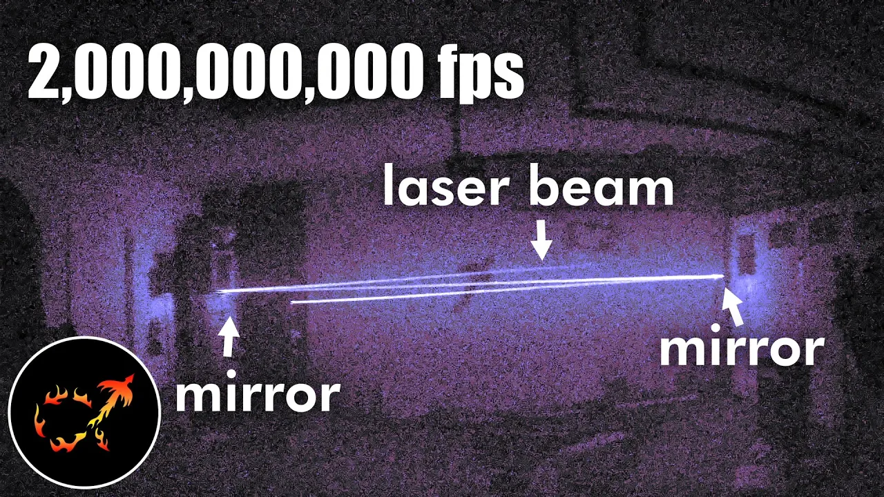
AlphaPhoenix 2B-FPS Camera Shows Geometry Alters Apparent Light Speed

AlphaPhoenix制作20亿帧/秒相机，展示几何位置如何改变光表观速度 由于有限的光子返回路径在空间中压缩或拉长了到达时间，表观光速会根据探测器位置在接近无限与减半之间波动。 AlphaPhoenix结合单像素光电倍增管、转向万向反射镜以及示波器的精确同步，制造出了一台拍摄速度达每秒20亿帧的超高速相机。拍摄在充满烟雾的车库中于多面反射镜间反弹的脉冲激光时，呈现出了一个表观悖论：背离相机传播的光看起来以半速移动，而返回的光似乎几乎瞬间穿过房间。事实证明，这一现象是来自空间不同点的光子飞行时间有限而导致的观测伪影，展示了探测器几何结构如何斜切时空。 AlphaPhoenix升级了他定制的高速成像装置，利用单像素光电倍增管搭配同步的双轴扫描镜，以每秒20亿帧（0.5纳秒间隔）捕捉高清视频。 (0:00) 该装置通过拼接由以3,000赫兹重复的同步15纳秒激光脉冲所产生的90多万个离散1x1像素时间序列，避开了对目前无法实现的数吉赫兹全画幅传感器的需求。 (2:29) 由于光的总传播时间等于到达散射体的路径加上返回镜头的路径之和，几何视角改变了表观速度：背离相机方向的光束看起来以半速传播，而返回相机的光束看起来几乎瞬间移动。 (23:09) 为了在受限于单通道模式的示波器上实现每秒20亿次采样，光电倍增管传感器测量和激光同步触发共用一条同轴线，并在时间上通过一条500纳秒的实体电缆延迟线隔开。 (20:15)

AlphaPhoenix demonstrates an upgraded custom camera capturing light propagation at two billion frames per second, revealing that observed variations in light speed across a room are optical artifacts created by finite signal travel times. Single-Pixel Scanning and HD Reconstruction (2:29) Recording full-frame video at two billion frames per second is economically and technologically inaccessible with conventional sensor arrays. To circumvent this, the setup operates by recording high-speed video at a spatial resolution of 1x1 pixel. A focused laser diode pulses roughly 3,000 times per second for 15 nanoseconds per flash, while a stationary photomultiplier tube (PMT) records a one-dimensional time trace for each pulse. A two-axis mirror gimbal sweeps the field of view across hundreds of thousands of pointing angles, allowing over 900,000 synchronized traces to be tiled into a single 1280x720 video that emulates a massive, ultra-fast array. Precision Gimbal and Magnetic Mechanical Fuse (5:40) Because each mirror pointing position becomes a single pixel, image sharpness depends entirely on angular repeatability. The yaw axis utilizes a 12-bit magnetic encoder across 1,280 positions, while the pitch axis uses a timing belt reduction to counteract reflection geometry that halves angular resolution. To protect the motor gearboxes from high-inertia stops, software velocity and acceleration ramps were implemented alongside a custom magnetic torque limiter. Unlike springs that stiffen under tension, the limiter’s interlocking 3D-printed teeth and magnets release cleanly when torque exceeds magnetic attraction, decoupling the drive before the motor gears can strip. Single-Channel Multiplexing via Coaxial Delays (20:15) Light gathered by the scanning mirror passes through a 2 mm pinhole at the lens focal length, which isolates spatial pixels, and strikes a PMT. The resulting electron avalanche is converted into a voltage across a 50-ohm resistor and sampled by an oscilloscope at 2 GSa/s (every 0.5 nanoseconds). Because the oscilloscope achieves its maximum sample rate only in single-channel mode, AlphaPhoenix multiplexed the optical signal and the synchronization trigger onto a single transmission line. An unspooled 500-nanosecond coaxial cable delays the inverted laser feedback pulse, allowing the oscilloscope to capture the optical pulse first and log the trigger pulse hundreds of nanoseconds later without cross-talk or electrical interference. Propagation Geometry and Apparent Light Velocity (23:09) Footage of a laser bouncing between parallel mirrors reveals an apparent paradox: light traveling away from the camera appears to move at half its speed, while returning light appears almost instantaneous. This distortion occurs because total transit time includes both the path from the laser to the scattering fog droplets and the path from the droplets back to the detector. When light moves away from a sensor located near the laser, the return distance continually expands, effectively doubling the light's travel path. Conversely, light traveling toward the camera shortens the return path at the same rate it advances, creating the illusion of superluminal propagation. AlphaPhoenix emphasizes that these apparent velocity shifts do not indicate anisotropic physics, but rather demonstrate that ultra-high-speed imaging captures an oblique slice through time. This garage-scale delay effect operates on the exact principles Ole Rømer used in the 1670s to calculate the speed of light by observing Jupiter's moon Io across interplanetary distances.

科普创作者 AlphaPhoenix 研发了一套每秒 20 亿帧（2 Gfps）的高清超高速成像系统，通过记录激光脉冲在车库镜面间的往复弹射，揭示了光线在远离或迎向观测者时产生的“视速度”剧烈变异，证明这种反常现象并非物理光速发生变化，而是探测器接收信号的有限传播速度在几何空间中切出的时间投影效应。 单像素扫描与精密运动控制架构 (2:29) 在现有的民用技术与成本限制下，使用大面积二维感光阵列以每秒 20 亿帧的速度进行高清实时录制几乎无法实现。该系统采用单像素（1×1）时间序列拼贴技术，激光器每秒发射约 3,000 次脉冲，每次脉冲仅持续 15 纳秒，占空比仅为 0.01%，但在峰值瞬时亮度比肉眼所见高出约 7,000 倍。光电探测器保持静止朝向天花板，由上方安装的双轴反射镜云台精确偏转光路，通过逐点扫描将超过 90 万条严格同步的单像素时间序列拼合成分辨率为 1280×720 的高清视频。 为确保每个扫描角度准确对应一帧视频中的一个空间像素，偏航轴（Yaw）采用 12 位磁编码器，将 360 度圆周细分为 4,096 个位置，在 112 度的广角视场内提供 1,280 个独立扫描位；俯仰轴（Pitch）因反射镜倾角会使光线偏转角翻倍，因而引入同步带减速机构以提升角分辨率与结构刚度。针对扫描停止时高惯性云台打磨伺服电机塑料齿轮的问题，除在软件上调整速度曲线与 PID 参数外，系统还设计了一套由六个 3D 打印部件和四枚磁铁构成的磁性扭矩限制器作为机械保险丝。利用磁力随间距拉大而急剧衰减的特性，当轴向扭矩超标时互锁轮齿会瞬间脱开，避免了传统弹簧受拉力增强而卡死的缺陷。 纳秒级光学系统与单通道示波器复用 (13:51) 光路系统由单枚透镜与小孔光阑组成，透镜安装在螺纹调节柱内，通过在焦平面衬入白纸校准成像清晰度。针对视场角分辨率，理论计算最佳孔径为 1 毫米，但实际选用了 2 毫米激光切割小孔，以牺牲轻微清晰度为代价让四倍的光子通过。探测端核心为高灵敏度光电倍增管（PMT），即使完全密封在黑色外壳内，微弱的电脑屏幕背光泄漏也曾导致过载噪声，必须在全黑环境下工作。光子撞击光阴极经光电效应激发单电子，在倍增级真空级联约 22 纳秒后雪崩放大为约 100 万个电子，再经 50 欧姆负载电阻转换为电压信号。 为达到每秒 20 亿次采样的极限速率，数字示波器必须以 0.5 纳秒间隔在单通道模式下运行。为解决单通道同时记录光信号与激光同步触发脉冲的冲突，该方案采用外接 50 欧姆同轴电缆构建双向传输线路：PMT 信号经过示波器的高阻探针后向下游电缆耗散，而激光器发射瞬间拾取的反馈电流在反相放大后，被注入一条长达 500 纳秒的卷盘同轴延迟电缆。反向传输的延迟触发脉冲在测量光信号数百纳秒后才抵达示波器，在时域上彻底分离了触发噪声与微弱的光学强度波形，避免了高昂的多通道工业仪器成本。 光程几何与光速变异的视觉佯谬 (23:09) 在 2 Gfps 的帧率下，光在每帧（0.5 纳秒）内仅前行约 15 厘米（6 英寸）。当激光在车库两侧的平行反射镜之间多次折射并照射悬浮雾滴时，改变相机位置会引发反直觉的视觉异常：远离相机而去的激光束看起来移动极慢，而反弹朝向相机而来的光束却似乎以接近无穷大的速度瞬时穿过空间。AlphaPhoenix 强调，这种现象并不违背光速不变原理，相机记录的画面并非空间中某一绝对时刻的静态截面，而是探测器沿时间轴斜切出来的投影。 当光线射向远离相机的雾滴时，光子不仅需要完成从激光器到散射点的正向传播，其散射光还必须跨越相同增加的距离返回相机，导致探测器记录到的往返光程增加了一倍，视觉上的“视速度”因而降低至物理光速的一半（c/2）。反之，当光线迎向相机反弹时，光束前行的距离增量恰好被其返回相机光程的减少量所抵消，在时间戳上产生几乎同时到达的假象。将激光在平行镜面间往复弹射并拼合在同一画面中，便形成了超光速与严重减速交替并存的光学奇观。 相对论时间切片与罗默光速实验的微观重现 (26:55) 光速有限性决定了现实中任何探测系统接收到的信号都属于“过去”，常规摄影动辄千分之一秒的曝光时间抹平了空间深度的传播延迟。系统在雾气弥漫的房间内拍摄旋转迪斯科球的实验生动展现了这一相对论延迟效应：靠近相机的散射光线几乎瞬间在画面中成型，而射向后方车库墙壁的光斑却在数帧后才明显显现，清晰暴露出空间纵深所固有的时间滞后。 这一实验所展现的几何延迟机制，在原理上完全重现了天文学家奥勒·罗默（Ole Rømer）在 1670 年代首次定量测定光速时采用的方法。罗默当时利用地球公转轨道上不同位置导致的木卫一（Io）蚀食时间偏差推算光速，而 AlphaPhoenix 的装置则在普通车库的人类日常尺度上，直接捕捉到了光线在普通物体间移动的时间切片，直观佐证了同时性的相对性与观测局限。 该系统通过单像素机械重构技术，以低成本在宏观生活尺度上可视化了光速有限性造成的时空切片畸变。但该测量方案在物理上高度依赖激光脉冲发射与物理过程的严格周期重复性，无法用于记录非可控、单次触发的瞬态光学事件。

[26:55] AlphaPhoenix: We will never know exactly what the world looks like everywhere at the same instant in time. In fact, that whole question is sort of assuming that the same instant in time exists everywhere in the world and that doesn't even work.

[0:00] This is a camera that I built last year [0:02] that shoots at a billion frames per [0:04] second. What could possibly be cooler [0:06] than that? [0:09] A camera that shoots at 2 billion frames [0:11] per second. [0:13] In HD. This camera, consisting of one [0:16] mirror, one lens, two tubes, cables, one [0:20] of the weirdest camera flash bulbs [0:22] probably ever built, and a few hundred [0:24] lines of Python, is not only fast enough [0:26] to watch light move, it's fast enough to [0:29] see the past. [0:31] Think about the weirdness that that [0:32] might cause during this first demo. [0:34] After my video about the billion frame [0:36] per second camera, there were so many [0:38] suggestions in the comments for cool [0:39] things to set up. And today in the [0:41] garage, I have the most requested [0:43] experiment. This is a high-power laser [0:46] that I have actually focused this time, [0:48] and it shoots down to the other end of [0:50] the garage where I have a mirror, where [0:52] that beam bounces back into another [0:54] parallel mirror. So, this beam of light [0:56] is going to ricochet back and forth [0:58] until it finally misses a mirror and [1:00] hits the wall down there. This is what [1:02] that setup looks like with a long [1:03] exposure photograph on a camera, very [1:05] similar to what your human eye would see [1:07] if you were standing here with me. And [1:09] this is what that looks like at 2 [1:12] billion frames per second. Light moves [1:15] about 6 in or 15 cm per frame of this [1:19] video. This beam of light is traveling [1:22] at the universe's speed limit. Light in [1:25] any reference frame will never move any [1:27] faster or any slower than this speed. [1:30] But, what happens if I move the camera? [1:38] This clip looks dramatically different. [1:40] The light traveling away from the camera [1:42] appears much slower, and the light [1:44] traveling back towards the camera looks [1:46] dramatically faster, like almost [1:48] instant. And that's like really weird, [1:51] because I just finished saying that [1:53] light always goes the same speed no [1:54] matter what. So, if you have an idea as [1:57] to why the light in that clip looks so [1:59] strange, leave it in the comments while [2:01] the title card plays. Cuz in this video, [2:04] I'm going to show you how I built the [2:06] upgraded version of my ludicrously [2:09] high-speed camera, and we're going to [2:11] get to the bottom of this light speed [2:13] mystery. [2:15] [Music] [2:29] Today, I want to take a video of the [2:32] light leaving this laser, traveling [2:34] across this room, [2:37] through all of this, I was becoming [2:39] increasingly frustrated that lidar [2:42] works. Look at that. That is so fast. [2:45] How to tastefully illuminate my entire [2:48] garage with a single laser diode. [2:50] [Music] [2:53] Since then, I've upgraded, and now I [2:54] have this. I completely overhauled the [2:57] motion stage and optics train in order [2:59] to reliably record in HD. I got better [3:02] at signal processing, and all of the [3:04] electronics necessary to move data [3:06] really, really quickly between the [3:07] sensor and the computer in order to not [3:10] only reduce the noise, but also record [3:12] at twice the frame rate. This is a [3:14] side-by-side comparison of the disco [3:16] ball shot from the first video. [3:18] [Music] [3:26] New one looks a lot better. [3:30] In order to explain what was bad about [3:32] the original camera and what's improved [3:34] about this setup, I kind of need to [3:36] explain how I'm able to record at a [3:39] billion frames per second. Basically, if [3:41] you want to record video at a billion [3:43] frames per second, you pretty much [3:45] can't. Not at any reasonable resolution, [3:49] with any reasonably accessible consumer [3:50] technology, for any remotely reasonable [3:53] price, which is why setups like this [3:55] kind of cheat. A lot of the comments on [3:57] the first video, I guess really on the [3:59] short that didn't have time to fully [4:01] explain everything, thought that this [4:03] was a stroboscopic technique, where it [4:06] was like a time lapse. I was just taking [4:08] discrete pictures and then putting them [4:10] one after each other. But, that's not [4:12] how this setup works. This camera and [4:14] the new camera over there are literally [4:17] capable of recording a video at a [4:20] billion frames per second or 2 billion [4:22] frames per second. [4:23] The catch is that it's only a one-by-one [4:26] pixel video. That's right. I can only [4:28] record one pixel at a time. So, when [4:30] that laser turns on, this camera may [4:33] record a video that looks like this. [4:36] Very exciting. [4:38] In order to build up a useful image, I [4:39] have to point the camera in a bunch of [4:41] different directions and record a bunch [4:43] of separate one-pixel videos. Every one [4:46] of these videos is a video of a distinct [4:49] event. It did not happen at the exact [4:51] same moment in time. But, if all of [4:53] these videos are synchronized, and we [4:55] take many, many, many one-pixel videos, [4:59] we can tile these videos next to each [5:01] other and play them all back at the [5:03] exact same moment and get something that [5:06] looks like a video. That tiling process [5:09] gives us a real, accurate representation [5:11] of what a true 2 billion frame per [5:14] second camera would see if, instead of [5:16] recording the data one pixel at a time, [5:19] we had like over 900,000 of these [5:22] sensors all pointed in different [5:24] directions from the camera, and we [5:26] recorded a single shot event with all [5:28] the data coming in at once. That's just [5:30] a significantly more expensive way to do [5:33] it, and it really wouldn't give us any [5:34] better of a result. [5:36] [Music] [5:40] Since the light sensor I'm using is [5:42] pretty sensitive considering what we're [5:43] asking it to do, and this whole printed [5:45] assembly is pretty heavy, I basically [5:47] just have my single pixel camera pointed [5:50] at the ceiling, and then the view from [5:51] that camera is guided around by this [5:54] gimbal-mounted mirror. Every unique [5:56] direction that I can point this mirror [5:57] in becomes its own pixel in the final [6:00] image. So, pointing precision and [6:03] repeatability are like ludicrously [6:05] important upgrades that differentiate [6:07] this camera from that camera. The [6:09] original camera had the mirror being [6:11] direct driven in both axes by these sort [6:13] of janky hobby servos, and the whole [6:16] assembly was on this, you know, wobbly [6:18] quarter-20 all-thread mount. It wobbled, [6:21] it drifted, it would break if you looked [6:23] at it funny. Now, I want to keep [6:25] improving this camera, especially the [6:26] space Oh, god, did I just snap [6:29] something? [6:31] Oh. In the last video, I asked for [6:34] suggestions, and many of you recommended [6:35] a specific type of servo with a built-in [6:38] encoder. In order to get an HD picture, [6:40] a minimum of 720 pixels tall by 1280 [6:43] pixels across, I needed to have some [6:45] pretty darn good angular resolution on [6:47] my mirror. A 12-bit encoder breaks the [6:50] 360° rotation up into 4096 different [6:54] directions. So, by direct driving the [6:56] yaw motor, I can get 1280 different [6:59] values by swinging the motor through a [7:01] 112° arc. That's a pretty reasonable [7:03] field of view, comparable to a regular [7:06] camera with a wide-angle lens, like the [7:07] one that you're viewing me on right now. [7:09] So, that works, but it just barely [7:12] works. And for the pitch motor, it won't [7:15] work. For the pitch motor that tilts the [7:17] mirror up and down, I not only needed [7:19] more stable pointing, but my angular [7:21] resolution was cut in half. Think about [7:23] a beam of light bouncing off a mirror. [7:25] If I tilt that mirror by 5°, the path [7:28] light will take bouncing off that mirror [7:31] changes by 10°. It gets doubled because [7:33] there's an angle on both sides of the [7:35] mirror normal. To handle this, I thought [7:37] about gears, I considered mechanical [7:38] linkages, I thought about getting a [7:40] higher resolution encoder on the motor, [7:42] but eventually settled on timing belts [7:45] and pulleys. I was initially worried [7:47] that belts would stretch and wouldn't be [7:49] accurate for exact pointing. But, I [7:51] actually found a paper where the [7:52] researchers tested exactly this, the [7:55] repeatability of angles achieved with a [7:57] belt drive, and they said it was cool. [7:59] Science is awesome. So, now with the [8:01] belt drive system, a large and easily [8:03] controllable motion of the motor becomes [8:05] a small and precise motion of the [8:07] mirror. I collect data in horizontal [8:09] lines, and while the mirror sweeps from [8:11] side to side, the laser light is [8:13] blinking on and off repeatedly. Using a [8:16] regular high-speed camera and some [8:18] split-screen cheating to film the [8:19] home-built ludicrous speed camera, this [8:21] is what that looks like. The mirror [8:23] spins so slowly that each time the laser [8:26] blinks on, the mirror is effectively [8:28] stationary for the duration of the [8:30] measurement. The light blinks on and off [8:31] almost 3,000 times per second, but the [8:34] laser is only on for about 15 ns at a [8:37] time. This means the light is actually [8:39] off for literally 99.99% [8:43] of the time. And while it's on, it's [8:45] about 7,000 times brighter than it [8:48] appears to a regular camera I'm filming [8:50] with now or to the naked eye. Your eyes [8:52] do an awful lot of averaging. This new [8:54] motion stage required a lot of trial and [8:56] error, mostly self-inflicted. My, let's [8:59] call it, frugality decided that these [9:02] tiny, cheap, plastic motors were [9:03] probably okay to swing around this big, [9:06] heavy assembly with a large moment of [9:07] inertia. [9:10] Go. [9:13] Geez. [9:17] God, that sounds awful. [9:19] Turns out that when you get the whole [9:21] swivel assembly swiveling, and then the [9:23] motor tries to lay on the brakes, the [9:25] big swivel assembly keeps on swiveling. [9:28] Yeah, that's broken. And in this case, [9:30] it shredded at least one of those little [9:31] tiny plastic gears inside the servo. I [9:34] shouldn't be able to pull teeth out of [9:36] my motor. I believe the correct answer [9:39] to this is actually a software fix to a [9:41] hardware problem. Hey, look at that. And [9:43] that's to just limit the acceleration of [9:45] the motor. The guts of this servo [9:47] actually can control limits for [9:49] velocity, acceleration, and some PID [9:51] tuning stuff on board, which is awesome, [9:53] even if I'm really bad at PID tuning and [9:56] I'm willing to accept some really [9:57] annoying bouncing at the end points. [10:04] And after figuring out which LLM code [10:06] snippets were useful and which LLM code [10:08] snippets were the reason I'd been [10:09] frustrated for hours, I got the motor [10:11] accelerating smoothly and decelerating [10:13] smoothly. So in normal operation, it [10:15] would never strip itself out. [10:17] Unfortunately, this is still software [10:19] fixed to a hardware problem and I was [10:20] not happy with it. There were still so [10:22] many ways for the system to crash and to [10:24] crash another motor. So I wanted a [10:26] torque limiter, but I couldn't find a [10:28] torque limiter or even a torque gauge [10:31] that went as low as the limits on this [10:32] motor. So I built both. This has been [10:35] bouncing around in my head for like the [10:36] last day and a half. I think I've got an [10:38] idea. This should be able to connect two [10:40] shafts. It should be able to unstick [10:43] smoothly and with a tunable amount of [10:47] stress because the magnets are going to [10:49] be far away. Using magnets instead of [10:51] springs means that when it starts to [10:53] spread apart, it'll spread apart much [10:55] faster, whereas springs, you know, get [10:57] tighter as you retract them. This [10:59] apparatus is made from six 3D printed [11:01] parts, four magnets, and some glue. [11:03] Really, it could have been two 3D [11:04] printed parts, but I was paranoid about [11:06] the layer lines getting stuck on each [11:07] other sideways, so I printed a little [11:09] teeth panel sideways, but the hub's flat [11:11] so the arms would be strong but [11:12] flexible. It's a whole thing. Basically, [11:14] if you ever try to turn the shaft too [11:15] hard, the bottom teeth exert a force [11:18] pushing the combs away from each other. [11:20] Once this force becomes large enough to [11:22] overcome the magnets holding them [11:23] together, the whole thing slides out and [11:25] is free to harmlessly spin. Now, with [11:27] the torque limiters installed, [11:31] even if this whole carriage crashes [11:33] somehow, the torque limiter breaks free [11:35] like a mechanical fuse and the motor [11:37] doesn't get shredded. Okay, now it's [11:39] mad. [11:40] Oh boy. [11:43] Now, all of that effort was just to [11:44] point a mirror, but all of the light [11:46] that bounces off this mirror eventually [11:49] finds its way into the optics train. [11:56] Actually, calling this an optics train [11:57] is a little aggressive. It's one lens [11:59] and one pinhole. I'm using a longer [12:01] focal length lens than I did last time, [12:03] but it's still just one lens. All the [12:05] light that comes in from one direction [12:07] then gets focused to a point by this [12:09] lens. In the last video, I equated this [12:11] pinhole to the aperture in a regular [12:13] camera lens, but [12:15] that's true, but it's really only true [12:17] for the out-of-focus light. In this [12:19] case, because I have the pinhole at the [12:22] intended focal length of the lens, it [12:24] would be more accurate to say that I'm [12:25] using this pinhole to set the pixel size [12:28] of my camera. I cut a variety of pinhole [12:30] sizes on the big laser and and they were [12:32] mostly round. [12:34] Uh [12:36] Yeah, I haven't actually fixed this yet. [12:37] So, [12:39] and although I cut out a whole bunch of [12:40] different pinhole sizes and calculated [12:42] that a 1 mm pinhole would be correct for [12:46] the amount of angular resolution that [12:48] I'm trying to achieve, I ended up going [12:50] with the bigger 2 mm one because I'm a [12:51] glutton for data and I was willing to [12:53] accept slightly fuzzier images as long [12:55] as I could cram four times as many [12:57] photons through that hole. The fun part [12:59] is that this lens is actually attached [13:01] to this big 3D printed column. You can [13:03] open it up to look at the focal plane. [13:05] You can spin the mirror up and down on [13:07] this big long thread in order to focus [13:09] the entire system. It's great. To get [13:11] the optics all trained in, you shine a [13:13] bright light at the scene, open the [13:15] doors, and set a white piece of paper [13:17] down in place of the pinhole. The light [13:18] coming in off the mirror gets focused [13:20] down to a nice little image on the paper [13:22] if you get the height of the lens just [13:23] right. And then we can lock the lens in [13:25] place with this ring. Since you want to [13:27] create as sharp an image as possible, we [13:29] want each pixel to be formed from the [13:31] light that only comes from one [13:33] direction. So we don't want to sample [13:35] the light from this entire image, just a [13:37] tiny piece of it. That's what this [13:38] pinhole is really doing. It's selecting [13:41] part of this image to analyze in each [13:44] measurement and blocking most of the [13:45] light with black cardboard. [13:47] Now, the light that does pass all the [13:49] way through the pinhole in the middle [13:50] makes it down to the sensor. [13:57] Okay, chapter two was pretty short, but [13:58] the electronics are the complicated [13:59] parts, so moving on. I'm using the same [14:01] photomultiplier tube as last time for my [14:03] light sensor. PMTs are awesome. They are [14:06] so ludicrously sensitive that they can [14:07] detect single photon events and vacuum [14:10] tubes are just gorgeous. So, when I [14:13] started adding electronics to this [14:14] project, I actually spent a couple days [14:16] thinking that my PMT was broken and I [14:19] literally had the page open to order a [14:21] new one. So last night I spent like two [14:24] hours fighting with the photomultiplier [14:26] tube and I could not figure out what was [14:28] wrong. I had like a ludicrous amount of [14:30] noise. Signal was terrible. All I wanted [14:32] to do was see a single photon show up in [14:34] the oscilloscope. I now have a single [14:37] photon showing up in the oscilloscope. [14:40] I forgot just how sensitive these things [14:43] are. Even though the entire thing is [14:46] closed off inside of opaque black [14:49] plastic, [14:51] these monitors are black, but they're on [14:55] and that's totally swamping it out. [15:01] There's a reason that last year I went [15:03] through the garage and covered every [15:05] window, every light, every little [15:06] indicator LED and I could only run [15:09] experiments at night. Once you get rid [15:11] of the vast majority of the light [15:12] though, you can get back to the world of [15:14] detecting individual photons. But for [15:16] now, just know that as light hits the [15:18] sensor, the intensity of that light is [15:20] converted to current in a wire. Current [15:23] that can be converted to a measurable [15:25] voltage with a 50 ohm resistor and fed [15:27] straight into this oscilloscope. [15:29] Oscilloscopes are really cool tools. [15:30] This is actually a brand new [15:32] oscilloscope, almost brand new after it [15:34] tried to cook itself. And if we plug [15:35] some wires into this marvelous [15:37] contraption, it can tell us the [15:39] electrical potential difference between [15:41] this probe and this clip at a rate of 2 [15:44] billion times per second. This is the [15:47] instrument that's literally collecting [15:49] and saving the data for this camera. [15:51] Imagine we have some time varying signal [15:53] passing into the scope on these wires. [15:56] Every half a nanosecond, the [15:57] oscilloscope looks at the signal, [15:59] measures it, and records the number [16:01] digitally in RAM. It's doing this all [16:03] the time, continuously saving data. But [16:06] if it receives a specific signal, like a [16:09] particularly strong or particularly [16:11] sharp signal, Woah. [16:14] then it stops recording, takes the saved [16:17] data, and plots it to the screen as a [16:19] value of voltage over time or in our [16:22] case, with data from this sensor, light [16:24] intensity over time. One really wacky [16:26] thing I want to point out is how long it [16:28] takes for information to pass through [16:31] this system. I'm going to animate over [16:32] this and I'm going to try to keep all [16:34] the speeds exact assuming that all the [16:36] signals are perfectly sharp, which [16:38] they're not, but bear with me. Imagine [16:41] that we have a photon that has left the [16:43] laser and it's traveling out into the [16:45] middle of the room at about 1 ft every [16:47] nanosecond. [16:49] That photon is going to scatter off the [16:51] droplet of fog that's suspended in the [16:53] air and it might redirect itself towards [16:57] the mirror over here. So it's going to [16:58] travel over also at about 1 ft per [17:01] nanosecond until it hits this mirror, [17:03] which is going to tilt it down and it's [17:05] going to pass through this lens. At that [17:07] point, it's inside the camera and [17:11] the lens to the sensor is almost 60 mm, [17:14] which means that it's going to take time [17:16] for that light after it has entered the [17:19] camera to reach the sensor. Four frames [17:21] of video worth of time just to move [17:24] through the camera at the speed of [17:26] light. Once that light reaches the [17:27] sensor down here, it impacts a piece of [17:30] metal, which releases a single electron [17:32] into the vacuum tube. That electron gets [17:35] bounced around between a whole bunch of [17:37] differently charged pieces of metal, [17:39] releasing a whole bunch more electrons, [17:41] turning our single event, our [17:42] instantaneous photon being absorbed [17:45] event, into a packet of like a million [17:48] electrons that all get dumped into the [17:50] wire at the same time. That whole [17:52] process inside the vacuum tube took [17:54] about 22 nanoseconds. And in the end, [17:57] that process just dumped a whole bunch [17:59] of excess electrons into this wire. Now, [18:01] since this wire already has electrons in [18:04] it and we've like crammed a whole bunch [18:06] more in one end, basically what happens [18:08] is that everybody has to take a step [18:09] forward. All the electrons in this wire [18:11] start moving and the useful information, [18:14] that signal, the rate at which all the [18:17] electrons start to take a step forward [18:20] is slightly slower than the speed of [18:22] light. I haven't actually measured the [18:23] velocity factor in this cable, but let's [18:25] assume it's like five or six [18:26] nanoseconds. At this point, I don't [18:28] actually know what the delay is, but [18:31] somehow inside that scope, it's [18:33] measuring the voltage on this wire. [18:35] Basically, the local scrunchiness of [18:37] electrons. If there's a lot of electrons [18:39] scrunched together, it's going to record [18:41] a large negative peak in voltage that we [18:43] interpret as light and that happens 2 [18:47] billion times per second and that data [18:49] is being stored digitally and then it [18:51] can be transmitted to the computer. If [18:53] we just zoom out and look at this [18:54] process, it is absurd to think about. If [18:57] we're recording a video with this camera [18:59] and we just saw recorded the fact that [19:01] the laser turned on and we call that [19:04] frame zero, the light entering the [19:06] camera lens at that moment contains [19:08] information about frame number 58. [19:11] Information about 57 frames of video are [19:14] moving through this camera at once. [19:17] Totally analog. By the time we've [19:19] recorded this frame, information about [19:22] this frame is here and at the wall, the [19:24] scene might look more like this. It's [19:26] like we're perceiving the world on a [19:28] delay. It's insane to think about. Like [19:31] if you froze time and looked at this [19:33] wire, you'd see scrunching of electrons [19:35] and say, "Ah, those are different frames [19:37] of video at the speed of electricity." [19:40] Absolutely wild. [19:42] [Applause] [19:47] To make sure that all the photon data we [19:48] record plays back properly, that all of [19:51] our one-by-one pixel videos start at the [19:54] same instant and we don't get something [19:56] like this where half the frame is on a [19:57] delay, we need an additional [20:00] synchronization or triggering signal [20:02] that can be measured by the oscilloscope [20:04] to give us a timestamp. Something to [20:06] register all of the data we collect back [20:08] to the moment that the laser turned on. [20:10] The last key leap of electronics that [20:12] allows this system to achieve 2 billion [20:15] frames per second without a truly [20:17] unreasonably expensive oscilloscope is [20:19] that I am both triggering the scope and [20:23] collecting data on the same channel. [20:26] Electrical engineers in the audience may [20:28] want to avert their eyes AT THIS TIME. [20:30] [Music] [20:32] THIS SCOPE can only hit 2 gigasamples [20:35] per second if I use a single channel. I [20:38] did not realize that when I bought this [20:39] scope, so I'm not just feeding the PMT [20:41] signal in and then terminating it with a [20:44] 50-ohm resistor. I'm actually [20:45] terminating that signal with another [20:48] 50-ohm cable pointed all the way over [20:50] there towards the laser. This means that [20:52] information from the PMT is actually [20:54] traveling down this cable [20:56] sort of past the scope and just straight [20:59] on into this cable. And as the [21:00] information scoots on by, the scope just [21:03] kind of looks at it. At the same time, [21:06] every time that laser blinks, there's a [21:08] current being fed through the laser [21:10] feedback signal that comes down one of [21:12] these wires and gets sent on to the [21:15] second board. You can see I planned [21:17] really well where that signal gets [21:18] inverted, amplified, and sent down here [21:20] into a significant quantity of coax and [21:23] then that heads over to the [21:25] oscilloscope. But that information is [21:27] traveling in on this line, so we [21:29] actually have data moving in two [21:31] directions through this piece of coax, [21:34] the at that point useless PMT data [21:36] that's just getting shot into hundreds [21:38] of feet of cable and the synchronization [21:41] data. The result of all of that is a [21:42] graph that looks like this where you get [21:44] all the PMT information about the [21:46] brightness of the light, then sometime [21:48] later a pulse that can be used to line [21:50] up all the videos after the fact. With [21:52] an added bonus that the synchronization [21:54] signal can't add noise during the [21:56] critical measurement because it's [21:57] literally too far away in time. This was [22:00] not easy to figure out and at least once [22:03] I had a literal shower thought that [22:04] became a bizarre Terminator setup. But [22:07] in the end, the answer was to invert the [22:09] timing signal so it had opposite [22:11] polarity to the PMT signal and [22:12] unfortunately eat some attenuation by [22:15] terminating both ends of the line with [22:17] 50-ohm resistors, but nothing at the [22:20] scope. In order to make these signals [22:21] reach the scope at different times, you [22:23] could design a really complicated delay [22:25] circuit to get exactly the time offset [22:27] you wanted or you could just buy another [22:29] 500 nanoseconds of cable. [22:32] I didn't even bother to unspool it. If [22:34] this cable section sounded like complete [22:36] soup to you, don't worry. I've got a [22:38] video about impedance matching that [22:40] actually got relegated to the second [22:41] channel because it was a little more [22:42] technical than the electricity waves [22:44] video that was on this channel, but you [22:46] should go check that out because I think [22:48] it's really fun. And in making that [22:50] video, I learned what I needed to know [22:52] to make this project possible. There is [22:54] no way that any of this would have come [22:56] together without me learning by making [23:00] that whole series about electricity that [23:02] I started a couple of years ago. [23:04] [Music] [23:09] Really slow. Really slow out there. Wow. [23:13] And on the way back, it's like one, [23:16] two, three. [23:19] Wow. Oh, that's perfect. I love it when [23:22] the data shows you exactly what you want [23:23] to see. Doesn't always happen. At the [23:25] beginning of this video, I said that [23:27] that camera could see the past. And to [23:30] be fair, every camera can see the past. [23:33] Your eye only ever sees the past. The [23:36] screen that you're watching this video [23:38] on right now lit up and it took a few [23:41] nanoseconds for that light to reach your [23:43] eyes before your eyes had any chance to [23:46] perceive that that light existed. But in [23:48] the vast majority of cases, this just [23:50] doesn't matter. My camera can take at [23:53] minimum 1/4000th of a second exposure. [23:56] That means that it is not only looking [23:58] at light that is immediately in front of [24:00] the camera, it also can look at light [24:03] from 50 miles away within the same [24:06] exposure. So regular cameras don't ever [24:09] have to deal with the propagation of [24:10] light because they just do too much [24:12] averaging. For all the ridiculousness of [24:14] the path that the information takes [24:15] through this camera, by the time the [24:17] information is in the camera, it's all [24:19] taking the same path, so it kind of [24:21] doesn't matter. This is not true, [24:23] however, for information traveling [24:26] outside the camera. This camera can [24:28] perceive the motion of light because [24:30] light traveling this path gets to the [24:32] camera faster than light traveling this [24:35] path. In the first case, light may take [24:37] 5 nanoseconds to get to a droplet of fog [24:40] in the air and then maybe 15 nanoseconds [24:42] to bounce all the way over to the [24:44] camera. And in the second case, maybe 15 [24:46] nanoseconds before it has hit some fog, [24:49] then 15 nanoseconds to get to the [24:50] camera. This extra path length is what [24:54] the camera perceives as a delay and it [24:56] only works perfectly because the path [24:59] back to the camera is the same length in [25:01] both cases. The camera is seeing the [25:04] light at this location and the light at [25:06] this location both 15 nanoseconds in the [25:09] past. If you look at this video and [25:11] think, "Wow, the light at the beginning [25:12] seems to be a tiny bit faster," then you [25:15] are really observant. It's slight, but [25:18] with this camera, the path light takes [25:20] to get to the camera is critically [25:22] important. When we point the camera in [25:24] different directions, what we're really [25:26] probing is this set of path lengths and [25:29] this distance to the camera is not the [25:31] same as this distance to the camera, so [25:34] things get weird. When we reposition the [25:36] camera to be behind the laser, this [25:38] effect is much more extreme. As the [25:41] light reflects from farther and farther [25:43] locations, it not only takes light [25:45] longer to get to the place where it [25:47] scatters, but it takes longer to get [25:49] back to the camera. Because we're [25:51] basically doubling the path length for [25:53] the light, the speed of light appears to [25:55] be almost half of its true value. If you [25:58] want to think about this another way [25:59] from some sort of classical objective [26:02] perspective, the camera sees things near [26:04] it with very little delay, but sees [26:07] distant objects farther and farther back [26:09] in time. The image formed by this camera [26:12] is not an objective view of the world at [26:14] a single moment in time, but a [26:16] perspective taking a slice obliquely [26:19] through time. For the light bouncing [26:21] back towards the camera or equivalently [26:23] if we put the camera at the far end of [26:25] the garage, we have the opposite effect. [26:27] If we look at the path lengths for each [26:29] position in this case, the total path [26:31] lengths are almost the same. As the [26:34] scattering location gets farther from [26:36] the light source, it also gets closer to [26:38] the camera. So we really can't detect [26:41] much of a difference in travel time. [26:43] With both mirrors set up so the light [26:45] can bounce back and forth many times, we [26:47] get to see both the artificial slowdown [26:49] effect and the artificial speed up [26:51] effect in the same clip and it looks [26:53] pretty trippy. I also need to point out [26:55] that this has nothing to do with the [26:57] actual speed of light changing or being [27:00] different in different directions. These [27:02] artifacts are the unavoidable result of [27:04] us sensing the world around us using our [27:07] eyeballs by absorbing radiation that has [27:10] a finite speed. We will never know [27:13] exactly what the world looks like [27:15] everywhere at the same instant in time. [27:17] In fact, that whole question is sort of [27:20] assuming that the same instant in time [27:22] exists everywhere in the world and that [27:25] doesn't even work. You can also see this [27:27] in the disco ball footage. The light [27:28] rays traveling towards the camera [27:30] through the fog from the disco ball show [27:32] up almost instantly and all the spots of [27:35] light where those rays actually [27:37] intersect the wall behind the disco ball [27:40] show up after a significant delay. [27:42] That's because the wall behind the disco [27:44] ball is farther from the camera, so [27:46] we're seeing it farther in the past. [27:50] [Music] [28:14] [Music] [28:18] I love this conclusion as a really weird [28:20] quirk of ultra ultra high-speed filming. [28:24] And a similar technique where the light [28:26] travel time to the observer was a [28:28] critical parameter was actually first [28:30] used to measure the speed of light by [28:32] Ole Rømer in the 1670s, but that was at [28:36] the scale of like planetary orbits and [28:38] this is at the scale of stuff in a [28:40] garage. It feels a lot more real to see [28:43] these effects play out with like human [28:45] scale objects. And now that I've got [28:47] this camera running, I'm planning on [28:49] making a whole bunch more videos with [28:51] it. So subscribe if you think that [28:52] sounds interesting and thanks for [28:54] watching. I'll see you next time. [29:02] [Music]