Stanford AI Predicts 25,000 Genes From Standard Cancer Biopsies
Stanford Online
Cross-modal foundation models can overcome clinical data shortages by accurately imputing high-dimensional molecular profiles directly from routine histology and generating synthetic volumetric radiology scans.
Stanford researchers developed Sequoia, a pipeline combining digital pathology foundation models and linearized Vision Transformers to predict expression levels of up to 25,000 genes directly from routine H&E histology patches. (7:38)
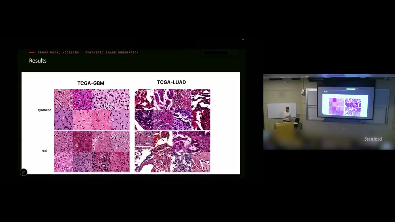
Conditioned cascaded diffusion models trained on VAE-compressed transcriptomic latents synthesized realistic H&E patches across 33 cancer types, generating over 30 million images that proved indistinguishable from real tissue to blinded pathologists. (17:09)
Standard autoencoders learned more clinically predictive latent representations from 3D brain MRIs than U-Nets, because skip connections let U-Nets bypass bottleneck compression and achieve high reconstruction similarity without capturing phenotype-rich features. (29:21)
A 3D generative framework combining conditional flow matching and Group Relative Policy Optimization (GRPO) reinforced with an external judge model improved pathology detection average precision on volumetric chest CT synthesis by up to 47%. (47:09)
Detailed notes
## Background
Published by Stanford Online on YouTube on November 3, 2026, this video records a lecture by Olivier Gevaert, an Associate Professor of Medicine and Biomedical Data Science at Stanford, delivered for the Stanford EE292R "AI and Data for Science" course. According to the page description, the session covers multimodal modeling for precision medicine, focusing on foundation models for cross-modal data imputation and synthetic data generation across spatial omics, digital pathology, and radiology to support in-silico investigations of disease mechanisms.
## TL;DR
Olivier Gevaert presents methodologies for integrating high-dimensional multi-omics, gigapixel histopathology, and 3D radiographic imaging to overcome clinical data scarcity and asymmetry. The talk highlights cross-modal biological imputation, showcasing vision transformers that predict genome-wide expression from routine H&E histology as well as diffusion pipelines that generate synthetic tissue patches from transcriptomic profiles. Gevaert also details 3D representation learning across massive brain MRI and chest CT cohorts, demonstrating how latent autoencoder embeddings, conditional flow matching, and reinforcement learning (GRPO) can simulate longitudinal disease progression and augment rare pathologies.
## Atmosphere & style
The presentation maintains a calm, intellectually rigorous, and grounded academic tone characteristic of an advanced Stanford graduate seminar. Gevaert delivers dense computational architectures with understated clarity, candidly acknowledging where models struggle, such as U-Net skip connections "cheating" past the latent bottleneck or transfer learning failing between adult and pediatric brain tumors. Interactive exchanges with the audience—probing image compression nuances, SSIM versus RMSE evaluation, and clinical validation hurdles—infuse the session with the collegial energy of active scientific debate.
## Bulletin
- [07:38](https://www.youtube.com/watch?v=GyjB3GYxEj0&t=458s) Stanford researchers developed Sequoia, a pipeline combining digital pathology foundation models and linearized Vision Transformers to predict expression levels of up to 25,000 genes directly from routine H&E histology patches.
- [17:09](https://www.youtube.com/watch?v=GyjB3GYxEj0&t=1029s) Conditioned cascaded diffusion models trained on VAE-compressed transcriptomic latents synthesized realistic H&E patches across 33 cancer types, generating over 30 million images that proved indistinguishable from real tissue to blinded pathologists.
- [29:21](https://www.youtube.com/watch?v=GyjB3GYxEj0&t=1761s) Standard autoencoders learned more clinically predictive latent representations from 3D brain MRIs than U-Nets, because skip connections let U-Nets bypass bottleneck compression and achieve high reconstruction similarity without capturing phenotype-rich features.
- [47:09](https://www.youtube.com/watch?v=GyjB3GYxEj0&t=2829s) A 3D generative framework combining conditional flow matching and Group Relative Policy Optimization (GRPO) reinforced with an external judge model improved pathology detection average precision on volumetric chest CT synthesis by up to 47%.
## Key takeaways
- [00:10](https://www.youtube.com/watch?v=GyjB3GYxEj0&t=10s) Multimodal fusion combining molecular sequencing, histopathology, and radiographic imaging consistently outperforms single-modality baselines across cancer survival prediction tasks.
- [05:13](https://www.youtube.com/watch?v=GyjB3GYxEj0&t=313s) The primary barrier to clinical translation of multimodal models is data sparsity, as routine patients rarely have matched datasets spanning radiology, digital pathology, and high-dimensional omics.
- [05:13](https://www.youtube.com/watch?v=GyjB3GYxEj0&t=313s) Because H&E histology slides are routinely collected in clinical standard of care while RNA sequencing is expensive, deep neural networks can use tissue morphology as a surrogate to impute missing molecular profiles.
- [12:59](https://www.youtube.com/watch?v=GyjB3GYxEj0&t=779s) Using domain-specific foundation model backbones like UNI paired with linearized Transformers enables accurate prediction of up to 17,000 genes from gigapixel whole-slide images.
- [12:59](https://www.youtube.com/watch?v=GyjB3GYxEj0&t=779s) Patch-level gene expression modeling allows models like Sequoia to generate spatially resolved transcriptomic maps across whole slides without requiring spatial transcriptomics pre-training.
- [17:09](https://www.youtube.com/watch?v=GyjB3GYxEj0&t=1029s) Cascaded diffusion models conditioned on 200 latent VAE parameters compressed from RNA sequencing can reverse the cross-modal direction, synthesizing high-fidelity histology patches.
- [26:48](https://www.youtube.com/watch?v=GyjB3GYxEj0&t=1608s) Pre-training diagnostic classifiers on synthetic histology images generated via diffusion outperforms training exclusively on limited real patient cohorts, specifically for rare disease subtypes and biomarkers like MSI.
- [29:21](https://www.youtube.com/watch?v=GyjB3GYxEj0&t=1761s) Evaluating multi-sequence 3D brain MRI compression across cohorts such as the UK Biobank revealed that standard autoencoders yield embeddings with far higher clinical and genetic correlation than U-Nets.
- [35:16](https://www.youtube.com/watch?v=GyjB3GYxEj0&t=2116s) Harmonizing approximately 35,000 public volumetric brain MRIs with standardized bias correction, skull stripping, and SRI24 atlas registration supports generalizable 3D foundation model encoders.
- [41:51](https://www.youtube.com/watch?v=GyjB3GYxEj0&t=2511s) Diffusion transformers conditioned on clinical parameters and flow matching simulate realistic multi-year longitudinal Alzheimer's disease trajectories, modeling structural ventricular enlargement and cortical thinning.
- [47:09](https://www.youtube.com/watch?v=GyjB3GYxEj0&t=2829s) Volumetric chest CT generative modeling utilizing flow matching and GRPO reinforcement learning surpasses NVIDIA's MAISI model across manifold coverage and pathology-specific detection metrics.
- [56:26](https://www.youtube.com/watch?v=GyjB3GYxEj0&t=3386s) Transfer learning across medical domains requires empirical validation; while representation transfer from common to rare pediatric brain tumors succeeded, transfer directly from adult glioblastoma cohorts to pediatric tumors failed.
## Detailed walkthrough
### [00:10](https://www.youtube.com/watch?v=GyjB3GYxEj0&t=10s) Agenda and Foundations of Multimodal Data Fusion
Olivier Gevaert begins by providing an overview of his lab’s research, setting up an agenda structured around three central themes: the motivation behind supervised multimodal modeling, methods for addressing missing modalities via data imputation and synthetic generation, and radiographic foundation models for 3D imaging. In biomedical data science, particularly in oncology, research initiatives have amassed extensive multi-omics databases—including RNA sequencing, microRNA profiling, clinical variables, and histopathology whole slide images—that can be synthesized computationally. Gevaert highlights an early 2019 project that applied neural network architectures to combine these disparate inputs for cancer patient prognosis. The resulting unified architecture mapped each data modality into a standardized 512-dimensional embedding vector, which was subsequently integrated to predict survival outcomes. Evaluated on large cohorts from The Cancer Genome Atlas (TCGA), this strategy proved that multimodal integration systematically outperforms unimodal baselines across multiple cancer sites.
```mermaid
flowchart TD
accTitle: Supervised Multimodal Architecture
accDescr: Multimodal inputs are passed into modality-specific neural encoders to produce 512-dimensional embeddings, which are fused to predict cancer prognosis.
subgraph Inputs["Patient Modalities"]
A["RNA-seq"]
B["microRNA"]
C["Clinical Data"]
D["Histopathology (H&E)"]
end
subgraph Fusion["Fusion Layer"]
I["Combined 512-D Embeddings"]
end
subgraph Output["Clinical Task"]
J["Patient Prognosis / Survival Prediction"]
end
A --> E
B --> F
C --> G
D --> H
E --> I
F --> I
G --> I
H --> I
I --> J
```
- TCGA represents a federally funded benchmark providing matched genomic, clinical, and imaging profiles across thousands of patients.
- Each diverse data modality was compressed into a dense 512-feature embedding vector prior to final outcome classification.
- Across multiple organ sites, combining features yielded superior survival risk stratification compared to isolated genomic or clinical models.
[02:21](https://www.youtube.com/watch?v=GyjB3GYxEj0&t=141s) Multimodal Fusion in Neuro-Oncology and Lung Cancer
Expanding beyond pan-cancer benchmarks, Gevaert details targeted applications in neuro-oncology and thoracic oncology. In adult and pediatric brain tumor studies, the lab fused RNA sequencing data—comprising the expression levels of approximately 25,000 to 30,000 human genes—with gigapixel histopathology slides measuring hundreds of thousands of pixels in each dimension. To tackle these multi-scale inputs, deep learning models were trained on hundreds of adult brain tumor cases and subsequently evaluated using transfer learning on rare pediatric brain tumor cohorts, where clinical data is inherently scarce. Gevaert outlines the classical taxonomy of data fusion paradigms: early fusion (concatenating feature representations directly prior to model layers), late fusion (training independent classifiers on each modality and aggregating their downstream decision scores), and intermediate fusion (learning joint latent representations within intermediate neural layers). In both brain tumors and a Stanford multimodal cohort of non-small cell lung cancer combining RNA sequencing, whole slide images, and 3D CT scans, multimodal fusion demonstrated a consistent advantage or clear positive trend over unimodal systems for predicting therapeutic response and overall survival.
> “Late data fusion on the other hand means that you build a separate model for each modality and then you integrate the decisions.” — Olivier Gevaert
- Molecular profiles measure gene expression activity across 25,000–30,000 protein-coding genes.
- Gigapixel whole slide images often span dimensions on the order of hundreds of thousands by hundreds of thousands of pixels.
- Transfer learning was leveraged to adapt adult brain tumor representations (trained on cohorts with hundreds of patients) to pediatric disease settings where sample sizes are severely constrained.
- In Stanford non-small cell lung cancer cohorts, tri-modal integration incorporated whole slide digital pathology, RNA sequencing, and volumetric CT radiography.
[05:13](https://www.youtube.com/watch?v=GyjB3GYxEj0&t=313s) The Challenge of Missing Modalities and Cross-Modal Imputation
Despite the proven predictive superiority of multimodal approaches, clinical translation is constrained by missing data. In real-world hospital workflows, patients rarely have complete, matched datasets spanning radiographic imaging, molecular assays, and histopathology. While high-dimensional RNA sequencing provides profound biological insight into tumor taxonomy and pharmacogenomics, it remains primarily an expensive research assay rather than a universal standard of care. Conversely, hematoxylin and eosin (H&E) histopathology slides are routinely prepared for virtually every diagnosed cancer patient worldwide. Because the molecular signatures and the stained histology originate from the very same physical tissue specimen, Gevaert’s team investigated whether deep neural networks could utilize routine H&E images as a direct surrogate to impute unmeasured molecular profiles.
> “So, we don't always have molecular data, imaging data, radiographic imaging data, clinical data for each patient. So we want to also develop methods that can either be robust against missing modalities or we want to develop methods that can impute missing data modalities.” — Olivier Gevaert
- Volumetric 3D radiographic image embeddings historically suffered from algorithmic bottlenecks and limited large-scale dataset availability, which has only recently started to improve.
- H&E histopathology is ubiquitous, cheap, and clinically mandatory, contrasting sharply with bulk and single-cell RNA sequencing.
- The fundamental premise of cross-modal histology-to-RNA imputation rests on the biological shared variance present within identical biopsy tissue sections.
[07:38](https://www.youtube.com/watch?v=GyjB3GYxEj0&t=458s) Predicting Gene Expression from Histology via Vision Transformers
To assess whether whole slide images could predict transcriptome-wide gene activity, the lab developed a Vision Transformer (ViT) pipeline capable of inferring the expression levels of approximately 25,000 human protein-coding genes directly from tissue morphology. Training was conducted across multiple organs using matched TCGA datasets (encompassing up to 10,000 cancer patients) alongside the Genotype-Tissue Expression (GTEx) portal to incorporate baseline gene expression profiles from normal, non-malignant tissues. Due to GPU memory limits, gigapixel slides (~200,000 × 200,000 pixels) were partitioned into patches of 250 × 250 pixels, which were systematically sampled across the tissue area and processed by the transformer architecture. The model was trained against bulk RNA sequencing ground truth (one continuous vector per entire histological slide) and subsequently evaluated on external validation cohorts, including proteomics datasets and spatial transcriptomics datasets that offer spatially resolved gene expression profiles across individual microscopic spots.
An audience member interjects to question the architectural necessity of tiling the images into small spatial patches:
> “200,000 by 200,000 that's a big image. Um there's a lot of ways to bring it down. I I don't know that every pixel actually matters. You're in the building where the compression people live. And so, I'm wondering are those images genuinely that big in the sense of their information content? Could they be compressed? Could you be Could you have taken them down by multi-scale resolution method compression? Was it really necessary to chop them into patches?” — Audience Member
Gevaert clarifies that while Whole Slide Images contain multi-scale pyramidal layers, pathologists routinely make definitive clinical assessments at 20× or 40× optical magnification. Consequently, preserving local high-resolution cellular architecture through patch extraction directly mimics the diagnostic standard of care while accommodating hardware memory constraints.
```mermaid
flowchart LR
accTitle: Histology to RNA Sequencing Vision Transformer Pipeline
accDescr: High-resolution histology slides are tiled into 250x250 patches and passed through a Vision Transformer to infer expression for 25,000 genes.
- TCGA provides multimodal training paired data for up to 10,000 oncologic patients.
- GTEx furnishes non-cancer reference baselines to map normative morphological-to-transcriptomic tissue relationships.
- Gigapixel slides are cut into 250 × 250 pixel patches to fit within transformer memory constraints while retaining fine-grained 20×–40× microscopic details.
- In bulk RNA sequencing training, a single global expression vector serves as slide-level supervision, whereas spatial transcriptomics provides localized coordinate-level validation.
[10:46](https://www.youtube.com/watch?v=GyjB3GYxEj0&t=646s) Multi-View Modeling and the Patch-Level Feature Extraction Pipeline
Responding to an audience question about multi-scale architectures, Olivier Gevaert affirms that multi-view models are a natural, largely untapped frontier for pathology images, drawing parallels to radiology where scans are viewed along axial, sagittal, and coronal planes. In histology, this equates to examining the tissue across different resolution levels: “I would say that multi-view models are definitely a next sort of step and have not been explored extensively.”
```mermaid
flowchart TD
accTitle: Whole Slide Image to Transcriptomic Feature Prediction Flow
accDescr: Pipeline decomposing a whole-slide histology image into patches, extracting features, clustering them to capture heterogeneity, and predicting a genome-wide expression vector.
subgraph Patches ["1. Patch Decomposition"]
WSI["Whole Slide Image (H&E)"] --> P1["250 x 250 Patches"]
end
subgraph FeatureExtract ["2. Feature Extraction"]
P1 --> F1["ResNet-50 Baseline (~200 dims)"]
P1 --> F2["UNI Foundation Model (~1,000 dims)"]
end
subgraph Clustering ["3. Heterogeneity Pooling"]
F1 --> CL["k-Means (100 Clusters)"]
F2 --> CL
end
The pipeline decomposes the gigapixel whole-slide image (WSI) into standard $250 \times 250$ pixel patches to stay consistent with ImageNet-trained backbones like ResNet. For feature extraction, the team compares a standard ResNet-50 baseline against modern digital pathology foundation models such as UNI, yielding feature vectors of roughly 200 to 1,000 dimensions per patch. Because cancer specimens exhibit high intra-tumor heterogeneity, sampling hundreds or thousands of patches per slide could overwhelm a model if not aggregated effectively; the features are therefore clustered into 100 centroids to capture distinct cell types and morphological niches before downstream inference.
- **Patch dimensions**: $250 \times 250$ pixels, maintaining parity with standard computer vision pre-training setups.
- **Feature backbones**: ResNet-50 (baseline) vs. UNI (specialized self-supervised vision backbone for pathology).
- **Heterogeneity modeling**: $k$-means clustering collapses thousands of individual patch representations into 100 representative cluster tokens.
- **Prediction heads tested**: A simple multi-layer perceptron, a standard Transformer, and a linearized Transformer.
- **Target output**: A 20,000-dimensional continuous vector representing full transcriptomic gene activity across the human genome.
---
[12:59](https://www.youtube.com/watch?v=GyjB3GYxEj0&t=779s) Benchmarking Sequoia Across Cancers and Validating Spatial Activity
When evaluating correlation between predicted and ground-truth RNA-seq profiles, domain-specific pre-training produces a marked improvement. UNI significantly outpaces ResNet, and the linearized Transformer outperforms standard neural nets and vanilla Transformers. In cancers with abundant training data—such as breast invasive carcinoma and bladder urothelial carcinoma—the architecture successfully predicts up to 17,000 individual genes with high correlation coefficients and low mean squared error. Conversely, for difficult tumors with limited sample sizes, such as glioblastoma, performance degrades:
| Cancer Type | Sample Availability | Predictive Performance |
|:--- |:--- |:--- |
| **Breast Invasive Carcinoma (BRCA)** | High (large patient cohort) | Up to ~17,000 genes predicted with high correlation and low MSE |
| **Bladder Urothelial Carcinoma (BLCA)** | High | Comparable high-accuracy genome-wide prediction |
| **Glioblastoma Multiforme (GBM)** | Low (aggressive brain tumor cohort) | Lower correlation and higher error due to limited training data |
Gevaert notes that their model, named Sequoia, outperforms prior published benchmarks on test sets from The Cancer Genome Atlas (TCGA) and sustains its predictive edge when cross-evaluated on the independent Clinical Proteomic Tumor Analysis Consortium (CPTAC) cohort. Furthermore, because Sequoia processes image tokens at the patch level, it can generate resolved gene-expression maps across the entire glass slide. Validated against a small spatial transcriptomics cohort of glioblastoma samples, the model reproduces spatial expression patterns for key marker genes across tumor tissue without ever having been explicitly trained on spatial transcriptomics.
Downstream clinical and translational use cases include:
- Imputing missing RNA profiles directly from standard-of-care hematoxylin and eosin (H&E) slides.
- Rescuing and profiling historical cohorts from concluded clinical trials where only formalin-fixed, paraffin-embedded (FFPE) glass slides remain.
- Stratifying patients into transcriptomic subtypes and feeding imputed expression profiles into established gene signatures to forecast therapeutic and drug response.
---
[17:09](https://www.youtube.com/watch?v=GyjB3GYxEj0&t=1029s) Inverting the Problem: Transcriptome-to-Histology Cascaded Diffusion
Having proven that images can predict transcripts, Gevaert turns the formulation on its head: can a genome-wide vector of 20,000–25,000 gene expressions synthesize a photorealistic, tissue-specific histology patch? Generative Adversarial Networks (GANs) frequently suffer from mode collapse and struggle to generalize across diverse tumor morphologies. To build a unified architecture covering multiple organs, the team implemented a conditioned cascaded diffusion framework inspired by text-to-image pipelines.
```mermaid
flowchart LR
accTitle: RNA-to-Image Cascaded Diffusion Architecture
accDescr: Pipeline mapping high-dimensional bulk RNA-seq data through a VAE bottleneck to condition a multi-stage cascaded diffusion model.
subgraph DiffusionStage ["Cascaded Diffusion Process"]
NOISE["Gaussian Noise"] --> D64["Base Diffusion (64 x 64 Patch)"]
LAT -.->|"Conditioning"| D64
D64 --> UP["Super-Resolution Diffusion"]
LAT -.->|"Conditioning"| UP
UP --> HRES["High-Resolution H&E Image"]
end
```
The model first compresses the 25,000-dimensional gene profile into 200 latent Gaussian parameters (means and variances) using a Variational Autoencoder (VAE). This compact vector conditions a base diffusion model that denoises Gaussian noise into an initial $64 \times 64$ pixel patch, followed by successive super-resolution diffusion stages to reach diagnostic-grade resolution. Trained across five cancer types, the generator yields histological features indistinguishable from genuine tissue: “And we showed these images to pathologists in a blinded way and they could not distinguish real versus synthetic data.”
---
[19:51](https://www.youtube.com/watch?v=GyjB3GYxEj0&t=1191s) Discussion: Information Overlap, Clinical Realities, and Spatial Limits
An audience member asks a conceptual question: if images can predict RNA-seq and RNA-seq can synthesize images, does that imply both modalities contain identical information? If so, why should medicine continue paying to measure both, and could clinicians quantify the truly orthogonal signals?
Gevaert acknowledges the apparent redundancy demonstrated by high cross-modal correlations, but clarifies that neither modality fully subsumes the other:
> “Well, sure. I agree that yes, because we are showing all this correlation between these two types of modalities. But that doesn’t mean that there’s no uniqueness about it, right? So that I think there’s still might be some value in each modality separately, especially looking at bulk RNA sequencing versus the image, right? Because we don’t have the spatial context in the molecular data model.”
He stresses that the clinical deployment reality is asymmetric: physical H&E tissue slides are ubiquitous, inexpensive, and mandatory for diagnostic pathology, whereas comprehensive RNA sequencing remains constrained by cost, laboratory infrastructure, and turnaround time. Imputing molecular data from existing glass slides bridges this diagnostic gap.
When asked whether bulk-conditioned models can resolve localized microenvironmental features—such as patches of chronic inflammation or focal immune infiltration—Gevaert clarifies that models trained on bulk RNA-seq have fundamental limitations regarding microscopic heterogeneity. Accurately untangling spatial heterogeneity requires training directly on true spatial transcriptomic datasets, which forms the basis of the ongoing research he introduces next.
[21:49](https://www.youtube.com/watch?v=GyjB3GYxEj0&t=1309s) VAE Dimensionality Reduction and Diffusion for Patch Generation
An audience member seeks clarification on the generative model architecture, asking whether a variational autoencoder (VAE) was used directly on the RNA sequencing data or whether the system behaves as a latent diffusion model. Olivier Gevaert clarifies the exact division of labor: the variational autoencoder operates as a distinct preprocessing module at the top half of the pipeline solely to compress the high-dimensional gene expression profile down to approximately 200 latent means and variances. Those latent representations are then fed directly as conditioning factors into the diffusion model to guide the synthesis of histopathology images.
```mermaid
flowchart LR
accTitle: Architecture for Conditioning Diffusion on Gene Expression
accDescr: Gene expression data is compressed through a VAE into a latent vector, which conditions a diffusion model generating histopathology patches.
subgraph Compression["Expression Encoding"]
A["Bulk / Spatial RNA-seq Data"] --> B["Variational Autoencoder (VAE)"]
B --> C["Latent Conditioning Factor<br/>(~200 means & variances)"]
end
subgraph Generation["Image Diffusion"]
C --> D["Diffusion Model"]
E["Noise"] --> D
D --> F["Synthetic Histology Patches"]
end
```
When asked whether clinicians noted missing spatial context when reviewing synthetic outputs generated from localized sequencing, Gevaert emphasizes a major technical parameter: the pipeline generates image patches rather than full whole-slide images. While synthesizing higher-resolution, full-slide images would be scientifically attractive, memory constraints and compute limitations make generating gigapixel whole slides directly via diffusion intractable, forcing the team to work at the patch scale.
[23:09](https://www.youtube.com/watch?v=GyjB3GYxEj0&t=1389s) Addressing Multimodal Data Scarcity Through In-Silico Synthesis
The discussion turns to earlier results where combining multiple modalities unexpectedly caused accuracy to drop for a specific cancer type. A student asks if this degradation stemmed from data scarcity and whether synthetic imputation could counteract the issue. Gevaert confirms this intuition directly:
> “That’s that’s exactly what we’re trying to do. So, we’re trying to one of the challenges is that multimodal cohorts are very scarce, right? So, we we it’s hard to find large amounts of data where we have exactly each modality collected for each patient.”
Because multimodal cohorts with complete paired data across every modality are rare, existing fusion benchmarks often show promising trends but lack the statistical power needed for definitive validation. Cross-modal generative models address this barrier by imputing unmeasured data, producing partially synthetic patient profiles, and generating augmented cohorts large enough to train robust supervised multimodal models.
A student then asks about the conceptual direction of the pipeline: whether the ultimate clinical goal is inferring molecular RNA sequencing directly from a standard tissue image, and why the lab is currently running the process in reverse by generating tissue images from transcriptomics. Gevaert agrees that predicting molecular properties straight from routine histology slides offers tremendous, easily deployable diagnostic utility because it uncovers molecular features invisible under standard microscopy. However, generating images from molecular data serves a complementary foundational purpose: it maps the mechanistic link from molecular states to tissue morphology, allows oversampling of rare conditions, provides high-volume data augmentation, and produces partially synthetic cohorts required to pre-train digital pathology foundation models. When asked if latent diffusion models could bypass the memory bottlenecks that prevent generating larger images, Gevaert acknowledges that performing diffusion within latent feature spaces is indeed a valid path forward.
[26:48](https://www.youtube.com/watch?v=GyjB3GYxEj0&t=1608s) Biological Fidelity Benchmarks and Scaling to 33 Cancer Types
To demonstrate that the synthetic patches preserve real biological morphology, the lab benchmarked generated images using HoVer-Net, an established segmentation and classification model that detects individual cell boundaries and identifies cell types. Comparing synthetic and genuine tissue patches across lung adenocarcinoma and kidney renal papillary cell carcinoma, HoVer-Net revealed matching cell-type distributions, verifying that the diffusion process correctly synthesizes complex microenvironments rather than generic histology textures.
```mermaid
flowchart TD
accTitle: Validation and Application of Synthetic Histology Patches
accDescr: Synthetic patches are evaluated with HoVer-Net, applied to clinical classification tasks, and scaled across 33 tissues.
subgraph Evaluation["Biological Fidelity"]
A["Synthetic Patches"] --> B["HoVer-Net Segmentation"]
B --> C["Cell Type Distribution Matches Real Tissue"]
end
subgraph Downstream["Downstream Tasks & Scaling"]
A --> D["Pre-training MSI Classifiers<br/>(Colorectal Cancer)"]
D --> E["Outperforms Real-Data Baselines<br/>in Accuracy & F1"]
A --> F["Scaled across 33 Tissues<br/>(30 Million Images)"]
F --> G["In-Silico Drug Perturbations & Rare Cohort Augmentation"]
end
```
The team tested whether synthetic data could improve downstream clinical task performance, evaluating microsatellite instability (MSI) prediction in colorectal cancer directly from H&E images. Pre-training image classifiers on increasing volumes of synthetic patches generated from RNA-seq conditioning outperformed baseline models trained strictly on real patient data in both accuracy and F1 score.
Building upon an initial version trained across five tissue types, the framework has now been scaled to 33 distinct cancer and tissue types, generating over 30 million synthetic histopathology images. Gevaert outlines the key use cases unlocked by this scale:
- **In-silico perturbation screening:** Simulating drug and molecular perturbations directly in tissue to inspect cellular alterations without physical assays.
- **Rare disease augmentation:** Oversampling scarce clinical cohorts, such as pediatric malignancies, where real-world biopsies are severely limited.
- **Treatment tracking:** Reading out morphologic responses, quantifying emerging or depleted cell types under therapeutic pressure.
- **Foundation model pre-training:** Benchmarking whether large foundation models trained on balanced mixtures of real and synthetic slides rival or surpass models trained purely on natural datasets.
[29:21](https://www.youtube.com/watch?v=GyjB3GYxEj0&t=1761s) Multimodal 3D Brain MRI Modeling and Representation Learning
Gevaert transitions to the lecture's second core theme: multimodal modeling in radiology, beginning with 3D brain MRI representations. He contrasts radiology with digital pathology, noting that while pathology now benefits from dozens of established foundation models, radiology foundation models remain nascent. Radiology faces severe heterogeneity across acquisition modalities (CT, MRI, PET), sequence protocols, and organ-specific anatomical geometries, making a single, generalizable "pan-radiology, pan-organ" model an ongoing challenge.
Brain MRI is inherently multimodal within a single examination session, acquiring multiple co-registered 3D sequences such as T1-weighted, T2-weighted, Fluid-Attenuated Inversion Recovery (FLAIR), and functional MRI (fMRI). The lab set out to train autoencoders capable of compressing these complex 3D volumes into dense feature representations—vectors containing several hundred to a few thousand values—that can be transferred to diverse downstream clinical tasks.
To ensure the learned representations generalize beyond single-institution cohorts or single disease profiles, the models were trained across large and diverse collections:
- **UK Biobank:** A population cohort of healthy volunteers, scaling from an initial 50,000 scans up to approximately 100,000 brain MRIs.
- **Neuro-oncology cohorts:** Multiple patient datasets capturing primary and secondary brain tumors.
- **ADNI (Alzheimer's Disease Neuroimaging Initiative):** Neurodegenerative disease cohorts tracking cognitive decline and structural brain atrophy.
- **Disconn cohort:** Specialized neuroimaging datasets focusing on schizophrenia and connectivity disruption.
The team evaluated four candidate architectures to compress brain MRIs: a standard autoencoder, a variational autoencoder, a U-Net, and an additional autoencoder variant. When assessing image reconstruction fidelity using the Structural Similarity Index Measure (SSIM), the U-Net substantially outperformed the other models. However, this apparent advantage exposed a fundamental flaw in using standard U-Nets for downstream representation learning:
> “And we found that not surprisingly, the U-Net is the best model to reconstruct the images in terms of the SSIM, the structural similarity index metric. But even though these models are capable of reconstructing the image, they're actually not good at learning this representation because they use these skip connections that essentially allow them to cheat and reconstruct the image, but this feature vector in the bottom neck layer doesn't really represent the [image]...”
By routing high-resolution spatial feature maps directly from encoder layers to decoder layers via skip connections, U-Nets bypass the bottleneck, producing visually sharp reconstructions while leaving the latent bottleneck vector impoverished and ineffective for downstream representation transfer.
[32:19](https://www.youtube.com/watch?v=GyjB3GYxEj0&t=1939s) Visual Perception Metrics vs. Pure Error in UK Biobank Autoencoders
An audience member interrupts to ask about image evaluation: "SSIM is a is a visual perception. And I'm wondering why you used that instead of root mean squared error." Olivier Gevaert acknowledges that they evaluate across multiple metrics, but emphasizes that their goal is to go beyond simple error calculations: "We have multiple metrics, right? But we wanted to also look at visual metrics instead of just pure error metrics." When the questioner clarifies, "In other words, you're modeling what a radiologist might see," Gevaert agrees: "Yes, exactly."
Turning to UK Biobank data, Gevaert explains how they evaluated whether the learned latent embeddings capture patient phenotypic characteristics. The UK Biobank encompasses extensive phenotypic data, including demographic information, volumetric measurements, vascular features, psychological profiles, toxic exposure data, and germline whole-genome sequencing. Comparing model variants across these diverse categories revealed that a standard autoencoder achieved the highest correlation with phenotypic traits, making it the top-performing model for capturing biological variation among participants.
- Evaluated phenotypic categories: demographics, volumetric and vascular features, psychology, toxic exposures, and germline genetic variants across the whole human genome.
- The standard autoencoder outperformed alternative variants in correlating with these diverse phenotypic categories.
---
[33:39](https://www.youtube.com/watch?v=GyjB3GYxEj0&t=2019s) Disease Prognosis and Downstream Clinical Predictions
Gevaert moves to clinical disease applications, testing how well the autoencoder embeddings generalize across patient cohorts. In an evaluation of overall survival across three independent brain tumor cohorts, the regular autoencoder proved most effective at stratifying patients into favorable and poor prognosis groups. The embeddings also predicted critical histopathological and molecular features directly from brain MRI scans without fine-tuning, including tumor grade and IDH1 mutation status (a key biomarker defining glioma subtypes).
Beyond neuro-oncology, the autoencoder representations transferred successfully to other disease areas:
- **Alzheimer's disease:** Subtype differentiation and prediction of APOE genetic variant status.
- **Schizophrenia:** Phenotypic and clinical feature prediction.
Gevaert highlights an important design trade-off: while U-Net architectures achieved superior low-level image reconstruction, the standard autoencoder was far more effective at learning condensed, biologically meaningful representations. “So while the U-Net was the best model to reconstruct these images a regular auto encoder was sort of this was the best model in terms of learning a low dimensional representation that then we can use sort of for dancing applications,” Gevaert notes. These learned brain MRI embeddings can subsequently be plugged into multimodal architectures alongside digital pathology and RNA sequencing.
---
[35:16](https://www.youtube.com/watch?v=GyjB3GYxEj0&t=2116s) Harmonizing 35,000 Brain MRI Volumes for 3D Foundation Models
Transitioning to recent work developed over the prior weeks and months, Gevaert discusses modernizing their pipeline. Earlier autoencoders were primarily limited to image reconstruction and relied on architectures that have since been superseded by vision transformers. Gevaert's lab set out to train a unified 3D encoder across massive public brain imaging cohorts, distinguishing their approach from common radiology models that still operate on 2D slices:
```mermaid
flowchart TD
accTitle: Brain MRI Harmonization Pipeline
accDescr: Flowchart illustrating the harmonization of thirty-five thousand brain MRI volumes across cohorts using standardized preprocessing.
subgraph RawData["Raw Multi-Cohort Data"]
A["35,000 Brain MRI Volumes<br>(GBM, AD, Healthy Aging)"]
end
subgraph Preprocessing["Standardized Preprocessing Pipeline"]
B["Bias Field Correction"]
C["Skull Stripping"]
D["Registration to SRI24 Atlas"]
end
subgraph StandardizedData["Harmonized Output"]
E["Standardized 3D Voxels<br>(Identical size & anatomical alignment)"]
end
A --> B
B --> C
C --> D
D --> E
```
To build this foundation model, the team assembled and harmonized roughly 35,000 MRI volumes from open-access databases spanning diverse clinical conditions—including neurodegenerative disorders like Alzheimer's disease and neuro-oncology cases like glioblastoma (GBM)—across broad age brackets. They standardized the disparate datasets using a unified preprocessing pipeline involving bias field correction, skull stripping, and spatial normalization to the SRI24 brain atlas, ensuring that corresponding voxels match the same anatomical coordinates across all patients.
- Cohort scale: ~35,000 3D MRI volumes across neurodegenerative, oncological, and normal cohorts.
- Preprocessing steps: bias field correction, skull stripping, and mapping to the SRI24 atlas for uniform voxel spacing and anatomical alignment.
- Comparable recent benchmarks mentioned: Brain-i-am (3D Vision Transformer) and NeuroChaP.
---
[37:54](https://www.youtube.com/watch?v=GyjB3GYxEj0&t=2274s) Flow Matching and Conditional Diffusion Transformers for MRI Synthesis
With harmonized volumes in hand, the team implemented a multi-stage framework. First, they trained a 3D masked autoencoder to tokenize brain MRI volumes into a low-dimensional latent embedding. To generate synthetic brain MRI scans from these latents, they replaced standard diffusion with conditional flow matching, which models the velocity vector fields from pure noise to structured latent distributions. Gevaert notes: “Instead of diffusion modeling, flow matching has been shown to be faster in terms of learning or generating realistic-looking images by learning sort of the velocity or the direction to go from noise towards real brain MRI latents.”
```mermaid
flowchart LR
accTitle: 3D Masked Autoencoder and Conditional Flow Matching Architecture
accDescr: Pipeline showing brain MRI tokenization via masked autoencoders followed by conditional flow matching image generation.
subgraph Stage1["Stage 1: Tokenization"]
A["Harmonized 3D Brain MRI"] --> B["3D Masked Autoencoder"]
B --> C["Latent Embeddings"]
end
subgraph Stage2["Stage 2: Conditional Generation"]
D["Conditioning Signals<br>(Sex, Age, Diagnosis, Scanner)"]
E["Gaussian Noise"]
C -.-> F["Conditional Flow Matching DiT"]
D --> F
E --> F
F --> G["Synthetic 3D Brain MRI Latents"]
end
```
The generation is conditioned using diffusion transformers (DiTs) informed by clinical metadata, demographic variables (such as sex and age), diagnosis status (healthy controls vs. Alzheimer's disease vs. brain tumors), and technical imaging acquisition parameters. Downstream validation confirmed that frozen representations from this 3D masked autoencoder, evaluated with a simple linear probe without fine-tuning, outperformed competing models at predicting IDH1 mutation status, tumor grade, brain age, and germline genetic variants.
Gevaert demonstrates how the conditional generative model can simulate longitudinal patient trajectories. Leveraging a dataset of approximately 25,000 training pairs and 3,000 validation pairs of longitudinal MRI scans, the model was conditioned to synthesize progressive anatomical changes over time. Starting from a baseline scan of a healthy subject, the diffusion transformer simulated the gradual transition into mild cognitive impairment and ultimately clinical Alzheimer's disease over multiple years.
Visual comparisons between normal aging controls and simulated Alzheimer's progression illustrate distinct structural patterns of progressive atrophy. Gevaert emphasizes that this work remains active and evolving: “And we're continuing to look how these model how we can validate these models. So, this is still work in progress. We have not done extensive validation yet of this generation.” He concludes by framing the broader objective: constructing robust multimodal representations across public datasets like the UK Biobank to empower downstream classification and reliably forecast future disease trajectories. He then pauses to invite audience questions before entering the lecture's final section.
- Longitudinal dataset: ~25,000 longitudinal brain MRI pairs for training; ~3,000 pairs for validation.
- Generative capability: counterfactual trajectory forecasting from healthy baseline to mild cognitive decline and Alzheimer's disease.
[43:53](https://www.youtube.com/watch?v=GyjB3GYxEj0&t=2633s) Clinical Validation and Latent Representations of Simulated Alzheimer's Brains
An audience member opens the discussion by asking about the clinical interpretability of the simulated Alzheimer's brain images. In clinical radiology, diagnosing Alzheimer's disease relies on distinct structural hallmarks, most notably the expansion of the cerebral ventricles—which the questioner points out as the prominent dark void expanding in the middle row of the slide—along with the progressive thinning of cortical gray matter. The audience member observes that while an autoencoder and U-Net architecture can capture the overall visual signature of an Alzheimer's brain, it is difficult to determine whether the network is merely mimicking known anatomical degradation or detecting subtle, previously overlooked biomarkers that human radiologists should be watching for.
Olivier Gevaert emphasizes that the longitudinal simulation project is in its infancy, having originated only months earlier, prompting lighthearted audience banter. Gevaert explains that evaluating and interpreting synthetic longitudinal scans presents significant hurdles because publicly accessible longitudinal imaging cohorts are exceedingly scarce and comparatively noisy. To validate whether synthetic aging reflects true neurodegeneration, Gevaert's lab has taken several indirect and direct approaches. First, they apply independent pre-trained diagnostic models—such as models calibrated to predict patient age—to the synthetic images to verify whether an artificially aged scan (for example, simulated 10 or 15 years forward) registers proportionally on external predictive benchmarks. Second, they plan to conduct rigorous blinded reader studies with expert neurologists and radiologists to assess whether clinicians can distinguish real from synthetic scans. Finally, they aim to implement feature attribution and backpropagation techniques to trace network activations back to the specific anatomical regions driving conditional predictions.
“So again, this is very early work. This is from a few months ago.” — Olivier Gevaert
“I'm very early in my life, too.” — Audience member
“And we deploy these models on synthetic data to see if we age a brain, let's say 10 or 15 years, do these other models that predict age, do they do they confirm sort of the synthetic data?” — Olivier Gevaert
- **Radiological Hallmarks Discussed**: Ventricular enlargement (the visible central dark fluid-filled spaces) and gray matter thinning.
- **Validation Modalities Planned**: Backpropagating model gradients to visualize salient anatomical regions corresponding to conditional disease flags.
---
[47:09](https://www.youtube.com/watch?v=GyjB3GYxEj0&t=2829s) Generative Modeling of 3D Chest CTs with Flow Matching and GRPO
Transitioning to his final topic, Gevaert presents recent work applying generative modeling to three-dimensional chest computed tomography (CT) scans. The radiology field has accelerated rapidly, driven by the release of massive public cohorts such as CT-RATE, which contains 50,000 chest CT volumes. Gevaert's team compiled and harmonized several public CT datasets into a unified pool to prevent the generative architecture from learning spurious technical artifacts across imaging sites. The core generative pipeline utilizes a frozen 3D Variational Autoencoder (VAE) to compress high-dimensional volumetric CT scans into a lower-dimensional latent representation, followed by a flow matching model conditioned on demographic variables, technical CT acquisition parameters, and clinical symptoms or disease findings such as pleural effusion.
```mermaid
flowchart TD
accTitle: 3D Chest CT Generation and GRPO Workflow
accDescr: Architecture showing 3D VAE compression, conditional flow matching, and GRPO post-training with a judge model.
subgraph Compression ["Representation Stage"]
A["3D Chest CT Scans"] --> B["3D Variational Autoencoder (VAE)"]
B --> C["Latent Space"]
end
subgraph Generation ["Generative Modeling"]
D["Conditioning Metadata<br/>(Demographics, CT Params, Findings)"] --> E["Flow Matching Model"]
C -.-> E
E --> F["Candidate Synthetic Scans"]
end
subgraph RL ["GRPO Post-Training"]
F --> G["Judge Model Scoring"]
G --> H["Relative Reward Assessment"]
H -->|"Policy Update"| E
end
```
To elevate the fidelity and anatomical correctness of specific pathology prompts, the team introduced Group Relative Policy Optimization (GRPO) reinforcement learning post-training. Given a specific prompt—such as a female patient of a particular age exhibiting pleural effusion—the generator produces multiple candidate scans, which are scored against the conditional requirements so the model learns policy adjustments that favor the most accurate samples. When evaluated against leading benchmarks, particularly NVIDIA's MAISI model, Gevaert's flow matching approach demonstrated superior distance metrics across both 2D and 3D measures, alongside higher sample density and coverage across the diverse manifold of lung CT appearances. Furthermore, GRPO post-training yielded dramatic empirical gains over baseline non-RL generation: average precision on pathology detection improved by up to 47%, while the area under the ROC curve increased by up to 24%. The team has generated and publicly released approximately 200,000 high-fidelity synthetic 3D chest CT images to augment rare pathology classes for training downstream diagnostic classifiers.
“And when we do reinforcement learning, we do improve the average precision up to 47%.” — Olivier Gevaert
- **Primary Benchmark Comparison**: NVIDIA MAISI volumetric generation model.
- **Key Dataset**: CT-RATE dataset comprising 50,000 volumetric lung CT scans.
- **Scale of Public Release**: Approximately 200,000 synthetic chest CT scans made available to the research community.
- **Downstream Utility**: Serving as targeted data augmentation for underrepresented disease findings to train robust diagnostic classifiers.
---
[52:17](https://www.youtube.com/watch?v=GyjB3GYxEj0&t=3137s) Lecture Synthesis, RL Judge Architecture, and Stanford Compute Infrastructure
Gevaert synthesizes the broader arc of his presentation by reviewing its four foundational pillars: multimodal data fusion as the core lab motivation, cross-modal biological imputation, 3D radiographic representation learning, and conditional generative modeling to synthesize volumetric radiology datasets. The lecture concludes with enthusiastic audience applause, leading immediately into a technical Q&A session focused on the mechanics of the GRPO reinforcement learning step and the computational resources behind the experiments.
An audience member asks for clarification on how the reward function is calculated during GRPO post-training and how the model determines which candidate scans are superior. Gevaert clarifies that the pipeline employs an external "judge model"—a pre-trained diagnostic evaluator that inspects each of the candidate synthetic scans generated for a given prompt, assesses how convincingly the specified finding is depicted, and supplies relative reward scores that update the generative flow policy. The conversation then turns to compute infrastructure and the heavy engineering burden underlying the research. Gevaert confirms that both the volumetric brain and lung generative models were trained on Stanford's Marla GPU cluster, noting that the BrainGen work alone consumed approximately 200 compute hours on NVIDIA H100 GPUs. In response to a final question regarding whether the immense data curation and harmonization efforts can be preserved for the broader Stanford community, Gevaert confirms that virtually all curated datasets and pipeline artifacts are being made publicly accessible online.
“Yeah, we have another judge model that actually looks at Yes. Yes. Yes, that's correct. Yeah.” — Olivier Gevaert
“I think the the brain gen work was about 200 hours on each 100s on Marla.” — Olivier Gevaert
“Yeah, I think virtually all these data sets that we have created we can make available online.” — Olivier Gevaert
- **Core Themes of Lecture**: Multimodal fusion, cross-modal imputation, 3D latent representation, and synthetic cohort generation for precision medicine.
- **RL Reward Mechanism**: An automated downstream judge model scoring candidate generations relative to conditional disease labels.
- **Hardware Footprint**: BrainGen models trained for roughly 200 hours on NVIDIA H100 GPUs hosted on the Marla cluster.
[55:18](https://www.youtube.com/watch?v=GyjB3GYxEj0&t=3318s) Data Sharing, Public Harmonization, and Clinical Deployment
The discussion begins with a dialogue around data distribution constraints and the feasibility of publishing research datasets versus providing the workflows to recreate them. Olivier Gevaert addresses the limitations imposed by republishing restrictions on public datasets, noting that releasing processing scripts allows researchers to reconstruct harmonized datasets on their own. A member of the audience suggests that outside tooling teams could assist in simplifying this process. Gevaert reflects on the evolving computational landscape, observing that recent tooling and specialized laboratory frameworks have drastically accelerated the aggregation of disparate public medical records: “I think this harmonization has been made easier using all the labs, right? It's a lot easier now to sort of harmonize public data in a fast way.”
The conversation then turns to whether multimodal algorithms are currently transitioning into active healthcare settings or if they remain distant milestones on research roadmaps. Gevaert explains that while widespread end-to-end multimodal systems are still nascent, discrete components have already found clinical utility. Segmentation models, especially within oncology pipelines designed to delineate tumors and segment healthy surrounding margins, represent clear examples of models that are actively deployed.
- Republishing restrictions frequently prevent direct dissemination of curated datasets, necessitating the distribution of pipeline scripts for reproducible local builds.
- Machine learning deployment in clinical oncology is currently anchored by automated anatomical and lesion segmentation (e.g., segmenting tumor boundaries versus normal margins).
---
[56:26](https://www.youtube.com/watch?v=GyjB3GYxEj0&t=3386s) Clinical Collaborations and Cross-Cohort Transferability
An audience member notes Gevaert's appointment in the School of Medicine and asks about direct collaboration with clinicians when evaluating synthetically generated diagnostic data. Gevaert confirms that clinical specialists actively evaluate their computational outputs, mentioning that his team has already carried out blinded reader evaluations with pathologists to evaluate synthetic tissue histology slides. He notes that comparable blind validation studies for the newer synthetic radiology models remain a near-term objective for the lab.
```mermaid
flowchart TD
accTitle: Pediatric Brain Tumor Transfer Learning Workflow
accDescr: Diagram illustrating the failure of adult GBM transfer compared to the success of transferring from common pediatric brain tumors to rare pediatric cohorts.
subgraph Adult["Adult Cohort Source"]
A["Adult Glioblastoma (GBM)"]
end
subgraph PediatricSource["Pediatric Cohort Source"]
B["Common Pediatric Brain Tumors"]
end
A -.->|"Transfer Fails (No cross-age generalization)"| Targets
B -->|"Successful Transfer (Shared pediatric biology)"| Targets
```
The Q&A shifts to model calibration and domain transfer across patient populations. When asked how one selects or calibrates which foundation architecture generalizes most effectively across neuro-oncology indications, Gevaert acknowledges the difficulty of establishing universal transfer rules. While initial hypotheses suggested that similarities in brain tumor presentation might allow models trained on adult glioblastoma (GBM) to adapt to pediatric cohorts, empirical evaluation demonstrated otherwise: “So we tried to transfer models, fusion models from GBM or adult brain tumors to these use cases which did not work, right? But, we could transfer from a more common pediatric brain tumor type to these two rare ones.” Adult tumor features failed to generalize to pediatric cases, but shared features across pediatric sub-types allowed successful transfer from common childhood brain tumors to rarer childhood diagnoses.
- Blinded reader studies have been conducted with certified pathologists to judge synthetic histology images, with radiology reader trials planned as next steps.
- Adult-to-pediatric transfer learning failed in neuro-oncology fusion models, while transfer learning across distinct pediatric tumor categories succeeded.
- Gevaert emphasizes that there is currently no simple rule of thumb to predict which medical domain transfers will perform well without empirical testing.
---
[58:15](https://www.youtube.com/watch?v=GyjB3GYxEj0&t=3495s) Data Asymmetry: Routine Histopathology vs. Molecular Profiling
An audience member raises a question about data availability, expressing surprise that the research leveraged larger volumes of imaging data than genomic or transcriptomic sequences, given the perception that sequencing data is relatively accessible. Gevaert clarifies that in real-world clinical care, imaging constitutes standard, routine patient intake, whereas comprehensive molecular assays remain exceptions due to infrastructure demands, high costs, and lack of universal insurance reimbursement: “So, the images are routine, right? So, these histopathology images are routinely collected in clinical practice versus the molecular data is not, right?”
Addressing why the group explored the inverse task—generating synthetic images from molecular profiles—Gevaert describes it as an inquiry into fundamental biological modeling. The work serves as a proof of concept for synthetic data augmentation and multi-scale systems biology, investigating whether models can bridge the hierarchical gap from cellular gene expression up to macroscopic tissue architecture. When an audience member remarks that any patient presenting with suspicious imaging would strongly desire confirmatory RNA sequencing, Gevaert agrees in principle, but underscores the practical constraints of wet-lab overhead, testing expenses, and clinical coverage policies that limit widespread sequencing in routine care. The lecture concludes with closing remarks and applause from the audience.
- Histopathology and radiology images are part of standard diagnostic workflows and are collected routinely.
- RNA sequencing and high-throughput omics remain constrained in frontline clinical settings due to turnaround time, wet-lab resource requirements, financial costs, and absent reimbursement pathways.
- Inverting the prediction pipeline (molecular profiles predicting or generating images) serves basic science goals, including multi-scale tissue modeling and algorithmic data augmentation.
## Notable quotes
> [37:54](https://www.youtube.com/watch?v=GyjB3GYxEj0&t=2274s) Instead of diffusion modeling, flow matching has been shown to be faster in terms of learning or generating realistic-looking images by learning sort of the velocity or the direction to go from noise towards real brain MRI latents. — Olivier Gevaert
## Mentioned
Olivier Gevaert, The Cancer Genome Atlas (TCGA), Genotype-Tissue Expression (GTEx), Vision Transformer (ViT), ResNet-50, UNI, Sequoia, Clinical Proteomic Tumor Analysis Consortium (CPTAC), HoVer-Net, UK Biobank, Alzheimer's Disease Neuroimaging Initiative (ADNI), Disconn cohort, U-Net, SRI24, Brain-i-am, NeuroChaP, CT-RATE, NVIDIA, MAISI, Marla, Stanford School of Medicine
## Video description
For more information about Stanford’s graduate programs, visit:
https://stanford.io/grad-ed-precision-med
This lecture is from Stanford EE292R AI and Data for Science, and it covers multimodal modeling for precision medicine, specifically focusing on using foundation models for cross-modal data imputation and synthetic data generation, and explores applications in spatial omics, digital pathology, and radiology that support in-silico study of disease mechanisms.
Follow the course schedule: https://aida4sci.stanford.edu/schedule.html#fall-2026
Speaker:
Olivier Gevaert is an Associate Professor of Medicine and Biomedical Data Science at Stanford.
Olivier Gevaert argues that while multimodal data fusion systematically outperforms single-modality baselines in clinical predictive tasks, translating these models into clinical workflows requires foundation architectures and generative models that bridge severe data asymmetry and missing modalities.
Supervised Multimodal Fusion and Domain Transfer (0:10)
Multimodal modeling in oncology combines molecular profiles, clinical metrics, and imaging data to enhance diagnostic and prognostic accuracy. Across The Cancer Genome Atlas benchmarks and Stanford non-small cell lung cancer cohorts, compressing disparate inputs—such as 25,000 to 30,000 gene expression features, microRNA profiles, and gigapixel whole-slide histology—into unified 512-dimensional embeddings yielded superior survival risk stratification compared to unimodal models.
However, real-world translation faces significant domain barriers and cohort scarcity. When evaluating transfer learning from adult glioblastoma cohorts to rare pediatric brain tumors, Gevaert's team observed that adult-trained models failed to generalize across age boundaries. Successful transfer instead required training on more prevalent pediatric brain tumor types, highlighting that biological differences can prevent cross-demographic model transfer despite shared organ anatomy.
Bi-directional Translation Between Histology and Transcriptomics (7:38)
Because routine hematoxylin and eosin (H&E) slides are universally collected whereas high-throughput RNA sequencing remains constrained by cost and infrastructure, Gevaert's lab developed methods to bridge this asymmetry. Their vision pipeline, Sequoia, decomposes gigapixel whole-slide images into 250 × 250 pixel patches, extracts features using pathology foundation models like UNI, clusters them into 100 centroids to capture intra-tumor heterogeneity, and predicts genome-wide expression vectors for roughly 20,000 genes. In breast and bladder cancers, the model accurately predicted up to 17,000 individual genes and reproduced spatial marker patterns without explicit spatial training.
Inverting the task, the team developed a conditioned cascaded diffusion framework that synthesizes photorealistic, tissue-specific histology patches directly from bulk RNA sequencing. The architecture compresses 25,000-dimensional profiles into 200 latent parameters via a variational autoencoder to guide iterative diffusion denoising. Validated using HoVer-Net cell-segmentation metrics and scaled across 33 cancer types to generate over 30 million images, synthetic patch pre-training surpassed real-data baselines in predicting microsatellite instability in colorectal cancer.
3D Brain MRI Embeddings and Progression Simulation (29:21)
Radiological foundation models face anatomical and protocol heterogeneity that makes volumetric 3D representation learning challenging. Evaluating autoencoders on the UK Biobank and neurodegenerative cohorts revealed a key representation trade-off: while U-Nets achieved the highest Structural Similarity Index Measure (SSIM) in image reconstruction, their skip connections allowed them to bypass the bottleneck layer, yielding representations that underperformed in downstream tasks. Conversely, standard autoencoders learned dense embeddings that correlated strongly with clinical phenotypes, survival outcomes, and biomarkers such as IDH1 and APOE mutations.
Building upon these latent representations, the team harmonized approximately 35,000 brain MRI volumes across cohorts using atlas registration and bias correction. Coupling a 3D masked autoencoder with conditional flow matching and diffusion transformers, the pipeline synthesized 3D volumes conditioned on age, sex, and diagnosis. Leveraging thousands of longitudinal MRI pairs, the generative framework successfully simulated structural progression—including ventricular expansion and cortical thinning—from healthy baselines to mild cognitive impairment and Alzheimer's disease.
Generative 3D Chest CTs via Reinforcement Learning (47:09)
To generate volumetric chest computed tomography (CT) scans, the lab combined 3D variational autoencoders with conditional flow matching across harmonized public datasets, including the 50,000-scan CT-RATE cohort. The generative pipeline incorporates demographic conditioning, scanner parameters, and targeted radiological findings such as pleural effusion.
To correct anatomical errors and improve prompt fidelity, the researchers introduced Group Relative Policy Optimization (GRPO) post-training. An automated external judge model scored multiple candidate synthetic volumes against specified disease labels to update the flow matching policy. This reinforcement learning step improved pathology detection average precision by up to 47% and AUROC by up to 24% over baseline non-RL generations, outperforming benchmark models like NVIDIA MAISI and enabling the public release of 200,000 synthetic 3D chest CT volumes for clinical data augmentation.
Gevaert emphasizes that while automated segmentation tools are already deployed in clinical oncology, end-to-end multimodal systems remain largely pre-clinical. Key unresolved challenges include republishing restrictions on medical datasets, the heavy compute burden of volumetric generation—such as the 200 NVIDIA H100 hours required for brain synthesis—and the need to complete formal blinded reader trials to prove clinicians cannot distinguish synthetic 3D radiology scans from genuine pathology.
[37:54] Olivier Gevaert: Instead of diffusion modeling, flow matching has been shown to be faster in terms of learning or generating realistic-looking images by learning sort of the velocity or the direction to go from noise towards real brain MRI latents.
Original transcript
[0:10] So, um I'm going to talk a little bit
[0:13] about some of the projects and some of
[0:14] the work
[0:16] we've been doing in the lab.
[0:17] And let me just dive right in.
[0:19] >> [clears throat]
[0:22] >> So, first I'm going to start with a
[0:24] little bit of background and motivation
[0:25] on supervised multimodal modeling just
[0:27] to set the stage.
[0:29] And then I'm going to already explain a
[0:31] little bit about
[0:33] missing data, especially missing data
[0:35] modalities and sort of methods that can
[0:38] be used for data imputation and
[0:40] synthetic image generation.
[0:43] And then
[0:44] the bulk of the presentation will be
[0:47] focused on our work in radiology
[0:50] and primarily in sort of developing
[0:52] models for radiographic [clears throat]
[0:54] images, 3D radiographic images, both
[0:58] foundation models and also models that
[1:00] can generate
[1:01] synthetic images.
[1:04] So, first let me give you a little bit
[1:05] of background in terms of multimodal
[1:07] modeling and multimodal data fusion.
[1:10] So, the idea of multimodal modeling is
[1:11] that you have multiple data sets of a
[1:13] patient. For example, in oncology, we
[1:16] often
[1:17] there is large databases and large
[1:19] projects that have collected data,
[1:21] multi-omics data, RNA sequencing data,
[1:24] microRNA data, clinical data, and
[1:26] images, histopathology images, that we
[1:28] can combine using machine learning. For
[1:30] example, here, this was a project we did
[1:32] a while back in 2019 where we used
[1:35] neural network models to combine all
[1:37] these different types of data for
[1:39] predicting the prognosis of cancer
[1:41] patients.
[1:43] So, essentially we developed a sort of a
[1:45] unified model that
[1:47] uses
[1:48] that learns an embedding for each of
[1:50] these different types of data that has
[1:53] 512 features, so 512 feature vector
[1:56] embedding, that then can be combined to
[1:58] make a prediction about the prognosis of
[2:00] cancer patients.
[2:01] Um
[2:02] and then we we showed that uh you can
[2:05] improve the performance
[2:07] um over single modality models across a
[2:09] number of different cancer sites, for
[2:11] example. And this is based on a large
[2:12] cohort uh from the Cancer Genome Atlas,
[2:15] which was a federally funded project
[2:16] that collected uh multiomic and imaging
[2:19] data for cancer patients.
[2:21] Similarly, um
[2:23] we have done also some uh work more
[2:25] deeply in uh certain uh diseases, in
[2:28] particular in neuro-oncology. Um this
[2:31] was a project we did on adult and
[2:33] pediatric brain tumors, where we
[2:34] combined two data sources, a molecular
[2:37] data source, which was RNA sequencing,
[2:38] and that gives you essentially
[2:40] um an activity level of all the genes in
[2:43] the human genome,
[2:44] uh which is roughly 25 to 30,000
[2:46] features, together with histopathology
[2:48] images. And these images are very
[2:50] high-resolution images. Uh often they
[2:52] have a few hundred thousand by a few
[2:54] hundred thousand um pixels. So, we uh
[2:57] were looking at these two very different
[2:58] types of uh data sources. Uh using
[3:01] essentially also uh deep learning models
[3:04] uh that can extract features from these
[3:06] uh two
[3:07] different types of data. And then we
[3:09] again want to make predictions. We want
[3:10] to um
[3:11] predict, for example, overall survival
[3:13] or prognosis. Um
[3:15] what I'm showing you here is uh three
[3:17] different cohorts because we want to
[3:19] These are complex models, so we need to
[3:21] train them on certain cohorts, we want
[3:22] to validate them on other cohorts. And
[3:24] then we also did a little bit of
[3:25] transfer learning here because we also
[3:27] wanted to show whether these models can
[3:29] transfer to pediatric disease uh because
[3:32] we have um we should train models in
[3:35] adult cancers, and you can see the
[3:37] numbers here, the patient numbers. We
[3:39] have hundreds of cases, uh but for
[3:41] pediatric disease, these are more rare
[3:43] diseases, so we don't always have enough
[3:45] data.
[3:46] Uh so, we want to test whether can we
[3:48] transfer models from one disease to
[3:50] another.
[3:52] Uh these are some uh results of this
[3:53] study where uh so, this is supervised
[3:56] data fusion, so we we essentially
[3:59] uh use early, late, and intermediate
[4:01] data fusion, where
[4:03] um
[4:03] these different types of data fusions
[4:05] are defined based on when you combine
[4:07] the data. Early fusion means that you
[4:09] concatenate the features
[4:11] and that's and you can see that each of
[4:13] these different types of data fusion
[4:16] outperform unimodal models.
[4:18] Late data fusion on the other hand means
[4:20] that you build a separate model for each
[4:22] modality and then you integrate the
[4:24] decisions.
[4:27] And then more recently we also have done
[4:28] some work on Stanford cohorts. This is a
[4:31] multimodal cohort of
[4:32] non-small cell lung cancer patients
[4:35] where we had multiple types of data.
[4:37] Similar data sets as before. We also
[4:39] have again RNA sequencing. We had
[4:42] histopathology images or whole slide
[4:44] images
[4:46] and we also had CT radiographic images.
[4:48] And again when we combine
[4:51] these images, when we combine different
[4:53] types of data to predict treatment
[4:55] response for these types of patients,
[4:58] we can show that combining the different
[5:00] modalities improves the performance or
[5:03] at least we have a
[5:05] a trend towards a better performance
[5:08] when multiple modalities are being
[5:10] combined.
[5:13] So that's sort of just to set the stage
[5:16] in terms of multimodal modeling and
[5:17] multimodal data fusion.
[5:19] But there's a number of challenges as
[5:22] was mentioned in the introduction. We
[5:24] don't always have all modalities for all
[5:25] patients. So we often lacking
[5:28] types of data. We don't always have
[5:31] molecular data, imaging data,
[5:34] radiographic imaging data, clinical data
[5:35] for each patient. So we want to also
[5:37] develop methods that can either be
[5:39] robust against missing modalities or we
[5:43] want to develop methods that can impute
[5:45] missing data modalities.
[5:48] And then secondly for a radiographic
[5:50] image data, learning embeddings of these
[5:53] types of images has been harder or has
[5:56] only recently been
[5:59] methods methods have been developed that
[6:01] are capable of extracting features
[6:04] in sort of a large scale, also due to
[6:06] the lack of data. And more and more data
[6:09] sets have been emerging recently that
[6:11] can be used to train
[6:13] complex models that can extract features
[6:15] and can be used for this type of data.
[6:21] So, first, let me
[6:22] talk a little bit about what we call
[6:24] cross-modal modeling where we impute
[6:26] missing data modalities.
[6:30] So, as I mentioned, some modalities are
[6:32] more routinely acquired than others,
[6:34] especially in routine clinical medicine.
[6:37] The use cases I will have here are in
[6:39] oncology,
[6:40] and certain modalities are routinely
[6:42] collected for each cancer patients, but
[6:44] others are not. For example, RNA
[6:46] sequencing is a molecular data modality,
[6:48] but is not routinely acquired for every
[6:51] patient. It's more of a research tool.
[6:54] But at the same time, it has a lot of
[6:57] validity and it's
[6:59] and value because it helps us subtype
[7:01] disease. It also helps us to determine
[7:03] what drugs you want to give to a certain
[7:05] patient.
[7:07] We We can get some insight into the
[7:09] biology of these patients, and so on.
[7:12] At the same time, H&E images,
[7:15] histopathology images, are part of the
[7:17] clinical cornerstone of diagnosis of
[7:19] cancer patients. So, we have these
[7:21] images clinically available for all
[7:23] patients.
[7:24] So, the question is, can we use that
[7:26] image as a surrogate for these molecular
[7:28] data? Because we know that the molecular
[7:31] features are generated from the same
[7:32] piece of tissue. How much correlation is
[7:34] there between these two types of data
[7:36] modalities?
[7:38] We developed developed a model that is
[7:40] capable of
[7:41] or that that wanted to evaluate to
[7:43] impute RNA sequencing data. And we
[7:46] tested we trained the model across a
[7:48] number of different tissues
[7:50] using a number of different databases. I
[7:52] already mentioned this database before.
[7:55] This is the cancer genome atlas
[7:57] database, which has up to 10,000
[8:00] patients with multimodal data. And
[8:02] specifically, the data modalities we are
[8:05] working with here are RNA sequencing and
[8:07] histopathology.
[8:08] And then there's another matched or
[8:11] another type of database which is called
[8:12] GTEx which has data for normal tissue.
[8:15] So, that gives us also sort of the
[8:17] normal baseline to train from. Um
[8:21] So, what the model is is essentially a
[8:23] vision transformer and it
[8:25] has as input these high resolution
[8:27] images which are again these whole slide
[8:29] images
[8:31] that are
[8:32] about 200,000 by 200,000 pixels.
[8:35] And so, we cannot fit these images in
[8:39] memory so we need to patch them. So, we
[8:41] create patches of 250 by 250 and then we
[8:44] sample across the whole slide.
[8:46] And that gets all fed into the vision
[8:48] transformer that then makes a prediction
[8:50] of about 25,000
[8:52] genes, protein coding genes that are
[8:54] known in the human genome.
[8:56] But we use some other data sets. This is
[8:58] another data set which also has protein
[9:00] data
[9:02] and has matched tissues.
[9:04] Then this is
[9:06] another data set for specifically for
[9:08] one cancer. So, these are two data sets
[9:10] we use for validation.
[9:12] And then we had some other
[9:14] data that we can use for validation in
[9:17] including a spatial transcriptomics
[9:19] cohort.
[9:20] So, in the the model is trained on what
[9:23] we call bulk RNA sequencing. That means
[9:24] that we have for the whole slide we just
[9:27] have one
[9:29] piece of ground truth. So, we have only
[9:31] one
[9:32] feature vector that captures the RNA
[9:34] sequencing.
[9:35] But in spatial transcriptomics we can
[9:37] actually also collect local ground truth
[9:39] on each spot in the slide and get a
[9:42] whole profile of all the genes in the
[9:45] human genome.
[9:46] >> Okay.
[9:47] Ask about your decision
[9:50] when you take these very large images.
[9:52] 200,000 by 200,000 that's a big image.
[9:55] Um
[9:56] there's a lot of ways to bring it down.
[9:58] I I don't know that every pixel actually
[10:00] matters. You're in the building where
[10:02] the compression
[10:04] people live.
[10:05] And so, I'm wondering
[10:08] are those images genuinely that big in
[10:10] the sense of their information content?
[10:12] Could they be compressed? Could you be
[10:15] Could you have taken them down by
[10:18] multi-scale resolution method
[10:20] compression? Was it really necessary to
[10:22] chop them into patches?
[10:23] >> So, the images are actually looked at at
[10:25] different resolution levels.
[10:29] And
[10:30] but typically pathologists look at a
[10:33] certain
[10:34] magnification, 20x or 40x, and we sort
[10:37] of mimicking that. And that's still
[10:40] means that we have a
[10:41] relatively high resolution.
[10:44] >> But but thinking for the students it
[10:46] might be a research project.
[10:47] >> Of course.
[10:49] I would say that multi-view models are
[10:52] definitely
[10:55] a next sort of step and
[10:57] have not been explored extensively.
[10:59] Similar models have been done in
[11:01] radiology where you also can do multiple
[11:02] views, actual, sagittal, coronal, and
[11:04] you could do something similar here but
[11:05] then at different resolution level.
[11:07] For sure.
[11:08] >> Thank you.
[11:09] >> I mean another aspect is that so we we
[11:11] are tiling the image into 50 by 250 just
[11:13] to be consistent with ResNet, right? So
[11:16] that's more or less just a consistency
[11:18] because then originally we were using
[11:20] sort of the the typical ImageNet based
[11:24] foundation models.
[11:28] So
[11:29] this is actually
[11:31] a little bit more detail about the
[11:32] model.
[11:34] So
[11:35] continuing with sort of these little
[11:37] patches, so these 250 patches,
[11:40] first of all, what we do is we need a
[11:42] feature structure and I just mentioned
[11:44] it so we can use ResNet 50 as a baseline
[11:47] feature extractor just to compare the
[11:48] models to.
[11:49] And then we're also using specific
[11:52] foundation models
[11:54] in the digital pathology space, for
[11:55] example, Uni,
[11:57] which recently emerged and outperformed
[12:01] a lot of the
[12:03] previous models.
[12:05] So that results then in a feature vector
[12:07] of 200
[12:09] or maybe 1,000 features, for example.
[12:12] And then because we know that the slide
[12:15] the sort of slide represents a piece of
[12:16] cancer tissue and we know that cancers
[12:18] are very heterogeneous. So, we want to
[12:20] capture the heterogeneity
[12:22] of these
[12:24] of the whole slide because we sample the
[12:25] slides maybe a few hundred or a few
[12:27] thousand times.
[12:29] So, then we get all these feature
[12:31] vectors and we cluster these into 100
[12:33] clusters.
[12:35] To capture that heterogeneity and
[12:36] potentially different cell types that
[12:38] are present in the slide.
[12:40] That is then fed into either one of
[12:42] these three models that we want to
[12:43] compare, a simple neural network, a
[12:45] transformer, and a linearized
[12:47] transformer that then has as output
[12:50] this
[12:51] 20,000 feature vector representing the
[12:53] expression or the activity of all genes
[12:55] in human genome.
[12:59] So, here are some results.
[13:01] So, we're comparing these two models.
[13:03] We're going to compare ResNet versus Uni
[13:05] each time for each of the three models
[13:08] that essentially summarize the
[13:09] expression.
[13:10] On the Y axis here, I'm showing you
[13:12] correlation coefficient. So, essentially
[13:14] how well the predicted expression for a
[13:17] single gene correlates with ground
[13:19] truth. And then on the right, I'm
[13:21] showing you how many genes
[13:23] we can predict with high correlation and
[13:25] low mean square error.
[13:28] So, what we found was that
[13:31] the Uni models or digital pathology
[13:33] specific foundation models for medical
[13:35] foundation models that trained on
[13:36] medical data on this specific type of
[13:38] data
[13:39] outperformed Uni ResNet
[13:41] significantly.
[13:43] And also the linearized transformer was
[13:45] a lot better compared to the other
[13:47] models.
[13:48] And you can see that we can actually
[13:49] predict
[13:51] many genes, thousands of genes. For
[13:53] example, this is breast cancer and these
[13:55] are bladder cancers. We can predict up
[13:57] to
[13:58] 17,000 genes with high correlation and
[14:01] low error just from the image.
[14:05] And this is true across a number of
[14:06] different tissues. There is a
[14:08] correlation with data set size.
[14:10] If you look at the breast cancer
[14:12] results, these are very good, but we had
[14:13] a lot of samples for breast cancer
[14:16] versus here glioblastoma which is the
[14:19] most aggressive brain tumor where we had
[14:21] a lot fewer samples and we see
[14:24] worse results for that cancer type.
[14:28] We also compared this model with
[14:30] previous models in this in this field
[14:32] and we showed that we can do better than
[14:34] previous work. This is on the test set
[14:36] within the TCGA and also on
[14:39] another validation data set which is
[14:41] this CPTAC data set.
[14:45] This is another
[14:47] validation where we look at how many
[14:49] genes are overlapping when we look at
[14:52] these seven tissues
[14:54] and how many genes we can actually
[14:55] validate when we train a model on one
[14:58] data set and then test it on the other.
[15:00] And and we see that the the overlap for
[15:03] the Sequoia model is a lot higher
[15:05] compared to for example the previous
[15:08] model in this space.
[15:11] And then finally
[15:13] we also because we are
[15:16] modeling actually the patch level and
[15:18] not the whole slide
[15:20] we can actually make a prediction at
[15:21] each patch. So on the whole slide we can
[15:24] actually
[15:25] visualize and look for each individual
[15:28] gene what its spatial activity is across
[15:31] a piece of tissue
[15:33] and that's what we did here for this
[15:35] glioblastoma cohort. So each first
[15:37] column here is a prediction for a
[15:39] particular gene in this row for a
[15:40] particular patient and the second column
[15:43] is the ground truth
[15:45] because we used so we had this small
[15:47] spatial transcriptomic validation cohort
[15:49] where we actually have spatial ground
[15:51] truth.
[15:52] And we found that even though the model
[15:53] was not specially trained we still could
[15:56] show a nice correlation
[15:59] across a number of cases and genes.
[16:04] So
[16:05] what can we do with this?
[16:08] So because we have routine H&E images in
[16:11] clinical practice we can now impute RNA
[16:14] sequencing data from these images and
[16:17] use that in various different use cases.
[16:19] For example, we can use it to stratify
[16:21] patients,
[16:22] to cluster patients for example, based
[16:25] on any cohort where we have these
[16:26] images.
[16:28] We can also we can impute expression in
[16:31] historical cohorts
[16:34] also from clinical trials for example.
[16:36] And we can also use it for example to
[16:37] predict drug response.
[16:39] We can look at
[16:40] computer profiles and feed them into
[16:42] expression based signatures
[16:45] of which
[16:46] there is a lot of them that reflect drug
[16:48] response.
[16:51] So to summarize, so this is what I just
[16:54] mentioned. So we developed essentially
[16:56] this vision transformer that is capable
[16:59] of
[17:00] predicting
[17:01] sequencing expression of up to 20,000
[17:04] genes and we validated that across a
[17:06] number of different tissues.
[17:09] So now we also ask the question, can we
[17:11] do the opposite? So can we use the
[17:14] feature vector of 25,000 features, these
[17:18] activity of gene expression values and
[17:21] can we generate synthetic images
[17:23] that reflect each tissue?
[17:26] And that's motivated by textual image
[17:28] models that have been popular in the
[17:30] past also in outside of medicine
[17:33] including for example generative
[17:34] adversarial neural network models
[17:37] but these some of these models have
[17:39] drawbacks. For example, guns are known
[17:41] to collapse
[17:43] and what we wanted to do to develop was
[17:45] a model that can capture many different
[17:47] tissues and single model single
[17:49] architecture that can essentially
[17:50] generate
[17:52] synthetic images across a number of
[17:53] different tissues.
[17:56] And then of course when you're
[17:56] generating these synthetic images, we
[17:58] need some ways to evaluate them. So we
[18:00] look at
[18:02] can we use synthetic data for
[18:03] pre-training for developing foundation
[18:05] models and also can we look at what
[18:08] cells are we detecting in these
[18:10] synthetic images and do they mimic real
[18:13] images?
[18:15] So we essentially
[18:16] mirrored
[18:18] the popular diffusion models which
[18:20] essentially allow to generate images
[18:21] from text
[18:23] Um and map that to sort of our use case
[18:25] where we have an RNA-seq vector
[18:28] that is being used as a conditioning
[18:30] vector in a cascaded diffusion model to
[18:32] then generate
[18:34] high resolution images that reflect that
[18:37] tissue.
[18:38] Here is the model. So first we wanted to
[18:41] reduce the dimensionality of the RNA
[18:43] sequencing data using a variational
[18:45] autoencoder
[18:46] and so we reduce the dimensionality to
[18:48] 200 means and variances that essentially
[18:51] captured the tissue from the
[18:54] transcriptome side.
[18:56] Then once we have this feature vector
[18:58] here, this 200 means and variances
[19:00] feature vector,
[19:02] we use that in a
[19:03] diffusion model where essentially we
[19:05] start from noise and we sample
[19:08] conditioned on this feature vector
[19:10] creating images and learning images of
[19:12] 64 by 64
[19:14] resolution and then up sampling this
[19:16] successively to the desired resolution.
[19:21] So we did this across initially across
[19:23] five tissues and we were able to
[19:25] generate synthetic images that
[19:28] faithfully reflected the different types
[19:30] of tissues. For example, here I'm
[19:32] showing you synthetic glioblastoma
[19:34] images, synthetic and real, and
[19:37] similarly lung adenocarcinoma images.
[19:39] And we showed these images to
[19:40] pathologists in a blinded way and they
[19:43] could not distinguish real versus
[19:45] synthetic data.
[19:47] Similarly, we then used other
[19:51] >> Sorry.
[19:53] So yes, I think it looks like you did a
[19:55] very good job predicting
[19:57] machine images. So like you
[19:59] you can predict RNA-seq from imaging and
[20:01] you can do the opposite. Does that mean
[20:04] they have the same information?
[20:06] But
[20:07] then why are we measuring both in the
[20:08] clinic? Is there a way to think about
[20:10] like
[20:11] It like it would be nice for decision
[20:13] making for clinicians that actually
[20:15] neither task is possible. They both have
[20:17] like orthogonal information.
[20:19] Is there a way to quantify that in this
[20:23] >> Well,
[20:25] Sure. I I agree that yes, because we are
[20:29] showing all this correlation between
[20:30] these two types of modalities.
[20:33] But that doesn't mean that there's no
[20:36] uniqueness about it, right? So that I
[20:38] think there's still
[20:39] might be some value in each modality
[20:42] separately, especially
[20:44] uh
[20:45] looking at bulk RNA sequencing versus
[20:47] the image, right? Because we don't have
[20:49] the spatial context in the molecular
[20:51] data model.
[20:53] Um but honestly, the the
[20:56] in current clinical practice, the the
[20:58] image is always available, right? And it
[21:00] will not go away. So we will always have
[21:02] that. It's more of the molecular side of
[21:03] things that is lacking behind in terms
[21:05] of being adopted in in routine clinical
[21:09] practice for diagnostics or for
[21:11] uh testing or biomarkers or for example.
[21:14] >> How good are you at predicting the
[21:17] heterogeneity? Like can you predict the
[21:19] areas that have a chronic inflammation
[21:23] >> So I I will talk a little bit about that
[21:25] at the end, I think. But so so the
[21:29] this model is based on bulk RNA
[21:32] sequencing.
[21:33] But if we have sufficient spatial
[21:36] transcriptomic data, we can model more
[21:39] faithfully each local structures within
[21:42] a slide.
[21:44] But that's that's work that we're
[21:46] >> So you're talking about the
[21:47] heterogeneity?
[21:47] >> Yes.
[21:48] >> The spatial heterogeneity.
[21:49] >> Spatial heterogeneity, exactly. Yes.
[21:52] >> I'm also a little confused about the
[21:54] model architecture in the previous
[21:56] slide.
[21:57] Is it a variational autoencoder used for
[21:59] the RNA sequence data or is it like a
[22:02] latent diffusion model?
[22:04] >> So the variational autoencoder is just
[22:05] to reduce the dimensionality of the
[22:07] expression data, and it's separate from
[22:09] the diffusion model, right? So the
[22:10] variational autoencoder is just is this
[22:12] first is a stop part, right? It's top
[22:14] half part. Essentially, we are using
[22:16] that just to reduce the dimensionality
[22:18] to let's say 200 means of variances, and
[22:20] then
[22:21] um
[22:22] that gets So that's that's this part
[22:24] here, right? And then this this is then
[22:26] just used here as a conditioning factor
[22:29] in the diffusion model.
[22:33] >> So,
[22:34] since this was locally sequenced,
[22:37] when you showed this to the clinicians,
[22:38] surely there's some missing spatial
[22:40] information. Did they point this out, or
[22:42] did they did they discover that, or
[22:45] I mean, did they did they see something
[22:47] which
[22:48] >> Um well,
[22:49] so we are we are not generating a whole
[22:52] slide, but we're generating patches. So,
[22:54] I think that's that's something that's
[22:55] very important to realize.
[22:57] We could potentially generate higher
[23:00] resolution images, but that's we get
[23:02] very [snorts] easily into compute
[23:04] restrictions, because it just there's
[23:06] just not enough memory.
[23:09] >> You mentioned a few slides ago that
[23:11] there's a correlation between the
[23:14] model efficacy, right? And there was a
[23:17] slight issue near the very beginning,
[23:18] right?
[23:20] And you showed [clears throat]
[23:21] improvements in in
[23:23] sessions of many different cancer types,
[23:24] but there's one specifically where a
[23:26] multimodal approach saw worse
[23:29] accuracy, I
[23:31] and I was curious if that's because
[23:33] there was like a lack of data for that
[23:35] specific cancer type, and that's why
[23:38] using different data sources
[23:41] caused a drop in accuracy, and if you
[23:42] tried any sort of this generative
[23:44] approach to improve that.
[23:47] >> That's that's exactly what we're trying
[23:49] to do. So, we're trying to
[23:52] one of the challenges is that multimodal
[23:54] cohorts are very scarce, right? So, we
[23:56] we it's hard to find
[23:59] large amounts of data where we have
[24:01] exactly each modality collected for each
[24:04] patient. So,
[24:07] and because of that
[24:09] a lot of the work in multimodal data
[24:10] fusion
[24:11] um
[24:12] it has has shown sort of like trends
[24:14] towards towards improvement and towards
[24:16] significance, and there are some success
[24:18] stories where you can really improve the
[24:20] performance,
[24:22] but there but we need more data to
[24:23] validate, and so on. So, yes,
[24:25] then these methods are
[24:27] the idea of these methods is to
[24:30] impute data to see whether we can use
[24:33] partially synthetic data or imputed data
[24:35] to increase cohorts and to
[24:38] test on larger samples for uh
[24:42] some of these supervised multimodal
[24:44] models.
[24:47] >> A quick question. So, on the at the high
[24:49] level, what do we want to do? We want to
[24:51] have a very good vision model where you
[24:53] give it a tissue image and it will give
[24:56] us a very accurate RNA sequencing of it.
[25:00] And then uh since you initially went
[25:02] this direction and then now we are
[25:04] having actually the opposite direction
[25:06] of it or are these synthetically
[25:08] generated images out of the actual RNA
[25:11] sequencing going to help us to improve
[25:13] the model
[25:15] uh
[25:15] training at the end? So, what are what
[25:18] do you
[25:18] >> Yes.
[25:18] >> opposite direction going to help us
[25:20] with?
[25:20] >> The I would say the short answer is yes
[25:22] to the first part of your question. Yes.
[25:23] So, um
[25:25] the the first part would be something
[25:27] that could be very easily deployed or
[25:30] would would have a lot of value in terms
[25:31] of generating missing or um
[25:35] uh
[25:36] features that cannot be appreciated
[25:38] using standard technologies, right?
[25:39] Which means from the image we could we
[25:41] could get uh a sense of the molecular uh
[25:45] properties of that tissue.
[25:46] Uh
[25:47] The this this work is more in terms of
[25:50] uh
[25:51] understanding the relationship going
[25:53] from molecular to to a tissue. And
[25:55] [clears throat]
[25:56] can for example help in terms of uh
[25:59] training models uh based on synthetic
[26:01] data. So, I will show this in next few
[26:03] slides. Also in terms of oversampling
[26:05] rare disease, for example. It's also a
[26:08] form of data augmentation where we could
[26:10] we can generate more synthetic data and
[26:13] partially synthetic data that can help
[26:15] in train uh train foundation models.
[26:17] Yes.
[26:18] >> Uh you mentioned running into like a you
[26:21] have to like generate patches because of
[26:23] compute issues. Have you tried using
[26:25] like a latent diffusion model to try and
[26:27] like get past some of these compute
[26:29] issues or have you guys experienced
[26:32] >> We could do some of this also in the
[26:33] latent space. Yes, that is true. Yeah.
[26:37] Let me uh continue a little bit further
[26:40] because some of this might also answer
[26:42] more or give more background on on these
[26:44] questions. Um, so this is uh one more uh
[26:48] analysis that we did to uh show the
[26:50] fidelity of these synthetic images. So,
[26:53] we used another AI algorithm called uh
[26:55] HoverNet, which is uh
[26:57] capable of uh detecting cells and
[26:59] predicting cell type. And so, what we
[27:01] wanted to do is to see whether the
[27:03] distribution of um
[27:06] cells was similar in synthetic data
[27:08] versus real data. And that's what you
[27:09] see here uh for lung uh adenocarcinoma
[27:12] and for renal cell uh papillary
[27:14] carcinomas.
[27:16] And then uh um similar to a previous
[27:18] question as well. So, we wanted to see
[27:19] can if we train a model or if we
[27:21] pre-train a model on synthetic data, can
[27:24] we improve uh um the performance of a
[27:27] classification problem? Uh, so here this
[27:29] is microsatellite instability prediction
[27:31] for colorectal cancer, which is a
[27:33] important clinical uh problem
[27:36] um from the image. And so, in blue I'm
[27:38] showing you uh a pre-trained model with
[27:40] synthetic data with increasing amounts
[27:41] of synthetic data. And we see that we
[27:43] can outperform uh models with real data
[27:47] um both in accuracy and F1 score.
[27:50] And then more recently uh we have
[27:52] extended this model. So, the original
[27:54] model was trained on five tissues and
[27:56] now we have extended this to 33 tissues
[27:59] um and we can essentially uh generate um
[28:02] faithful images for each uh tissue
[28:05] types.
[28:06] Um, so to uh mention some of the use
[28:09] cases, so
[28:10] we can uh potentially simulate
[28:11] perturbations. For example, for uh drug
[28:14] discovery, this can be important or can
[28:16] be relevant
[28:17] uh if we can faithfully capture
[28:19] perturbations with uh molecules, uh that
[28:22] would um
[28:24] allow in silico experiments. Um, we can
[28:27] also augment uh rare cohorts. For
[28:29] example, pediatric uh tumor types, we
[28:31] can oversample these um
[28:33] and we can also look at uh reading out
[28:36] response in tissue. We can look at uh
[28:38] synthetic data, look at what cells are
[28:40] there, and use that for uh tracking
[28:43] treatment.
[28:45] So, this is to summarize, um, this work.
[28:48] Um,
[28:49] so the idea here was really to, um,
[28:52] develop a model that can, uh, generate
[28:54] synthetic images, and then these can be
[28:57] used in the context, for example, of
[28:59] data augmentation. And this is something
[29:01] that we're doing right now. We have used
[29:02] this model across all these different
[29:04] tissue types to generate 30 million
[29:06] images, and we are testing whether
[29:09] mixtures of real and synthetic data can
[29:12] be used to train digital pathology
[29:14] foundation models, and how they
[29:16] benchmark, uh, with existing ones.
[29:21] So, now let me switch to the second
[29:23] part, um,
[29:24] of the presentation, which is focused on
[29:27] our work in radiology.
[29:29] Um, so first I want to give you a little
[29:31] bit of background on, uh, 3D brain MRI
[29:34] modeling. Um, and a study that we did
[29:37] already a few years ago was, uh,
[29:40] using autoencoders on radiology. And I
[29:42] already mentioned that the models for
[29:44] radiology are still nascent, so we we in
[29:48] in digital pathology space we now have a
[29:49] few dozen foundation models that have
[29:51] shown, uh, uh,
[29:53] excellent performance in various
[29:55] different tasks, whereas in radiology
[29:57] more and more models are still emerging.
[29:59] Also, because radiology is much more,
[30:01] uh, heterogeneous. Uh, we have CT, we
[30:03] have MR, there's also organ-specific,
[30:06] uh, features, and training sort of a
[30:08] pan,
[30:09] uh, radiology, pan organ model is still
[30:12] an out, uh,
[30:14] is still a challenge. Um,
[30:16] so we use sort of more older models, uh,
[30:19] autoencoders initially to represent, uh,
[30:22] multimodal brain MRI. Um, so it's
[30:25] important to mention that, uh, brain MRI
[30:26] is already multimodal. We don't just
[30:28] have one 3D image, we have multiple 3D
[30:31] images, that you want T2 flare, you can
[30:33] also have functional imaging.
[30:35] And the idea is that what what we wanted
[30:36] to do is we wanted to learn models uh,
[30:38] using autoencoders that
[30:41] represent brain MRIs in lower
[30:42] dimensional representation. For example,
[30:44] a feature vector of a few hundred or a
[30:46] few thousand features. And then we
[30:48] wanted to use that in downstream
[30:50] applications.
[30:52] And so here I'm listing the some of the
[30:53] datasets that we used
[30:55] to train these models and train various
[30:58] architectures with autoencoders.
[31:01] We used the UK Biobank, which is
[31:03] a database of healthy volunteers with up
[31:06] to 50,000 and recently has been
[31:08] increased to about 100,000 brain MRIs.
[31:11] Then we used a number of neuro-oncology
[31:13] cohorts.
[31:14] And one [clears throat] thing that we
[31:15] also did in this project, we wanted to
[31:17] show that these autoencoders can learn
[31:20] features that are relevant for multiple
[31:22] different diseases. So we tried we have
[31:26] cohorts in in oncology, but also
[31:28] neurodegenerative disease, which is this
[31:30] ADNI cohort, and schizophrenia, which is
[31:32] this disconnect cohort.
[31:35] So here are the four architectures that
[31:38] we evaluated. So we had a
[31:39] U-Net,
[31:41] variational autoencoder, regular
[31:43] autoencoder, and another one.
[31:45] So first we wanted to check whether
[31:47] these autoencoders can reconstruct
[31:49] original images.
[31:51] And we found that not surprisingly, the
[31:53] U-Net is the best model to reconstruct
[31:55] the images in terms of the SSIM, the
[31:57] structural similarity index metric.
[32:01] But even though these models are
[32:04] capable of reconstructing the image,
[32:06] they're actually not good at learning
[32:07] this
[32:09] representation because they use these
[32:10] skip connections that essentially allow
[32:12] them to cheat and reconstruct the image,
[32:14] but this feature vector in the bottom
[32:17] neck layer doesn't really represent the
[32:19] image very well.
[32:20] >> Can I just ask a quick question?
[32:22] >> Yes.
[32:22] >> Um
[32:23] SSIM is a is a
[32:25] visual perception.
[32:26] >> Yes, yes, it is.
[32:27] >> And I'm wondering why you used that
[32:29] instead of root mean squared error.
[32:31] >> We we use we use
[32:33] we have multiple metrics, right? But we
[32:35] wanted to also look at visual metrics
[32:38] instead of just pure error metrics.
[32:40] >> In other words, you're modeling what a
[32:42] radiologist might see
[32:43] >> Yes, exactly.
[32:44] >> I think I got you there.
[32:49] >> [clears throat]
[32:49] >> So now we wanted to see how well this
[32:52] embedding is capturing phenotypic data.
[32:54] So within UK Biobank a lot of phenotypic
[32:56] data is being collected. So we have a
[32:59] number of different categories,
[33:00] [clears throat]
[33:01] demographics, a lot of volumetric,
[33:04] vascular features.
[33:06] What's also important this is genetic
[33:07] database where we have germline genome.
[33:10] So we know all their
[33:13] genetic variation across the whole human
[33:15] genome. And then some other
[33:18] features such as toxics toxics and
[33:20] psychology.
[33:22] And so across all these different
[33:23] categories we found that the regular
[33:26] autoencoder in green has the best
[33:28] correlation with any of these feature
[33:30] categories.
[33:31] So this model was sort of the best in
[33:33] capturing sort of the the biology of
[33:36] these
[33:37] participants.
[33:39] So then in the second stage what we
[33:41] wanted to do is we wanted to see how
[33:42] well these models work in disease areas.
[33:44] So here I'm showing you overall survival
[33:46] prediction in three brain tumor cohorts.
[33:49] And again their regular autoencoder was
[33:51] the best model in splitting patients in
[33:54] terms of good or poor prognosis group.
[33:58] Similarly we could in the same cohorts
[34:01] we could predict some molecular features
[34:03] from the image or from the brain MRI. We
[34:05] can predict the tumor grade which is the
[34:07] histopathological feature.
[34:09] >> [clears throat]
[34:10] >> We can predict IDH1 status which is a
[34:12] genetic mutation that defines two
[34:15] subtypes in glioma
[34:17] and a few other features.
[34:21] >> [clears throat]
[34:21] >> And then in the two other disease areas
[34:24] we can predict subtypes in
[34:27] Alzheimer's disease
[34:29] and also the APOE genetic variant.
[34:32] And similarly for schizophrenia.
[34:36] So
[34:37] while the U-Net was the best model to
[34:39] reconstruct these images a regular auto
[34:42] encoder was sort of this uh
[34:45] was the best model in terms of learning
[34:47] a low dimensional representation that
[34:48] then we can use sort of for dancing
[34:50] applications.
[34:52] And we showed this across these three
[34:54] disease areas.
[34:56] And the idea now is that we can
[34:57] >> [clears throat]
[34:57] >> use these feature factors in multimodal
[35:00] models together with for example the
[35:02] model I showed you in the beginning
[35:04] on the brain tumor multimodal brain
[35:06] tumor example where we combined RNA
[35:10] sequencing with digital pathology data
[35:11] and now we can also model
[35:13] brain MRI.
[35:15] >> [snorts]
[35:16] >> So now
[35:17] continuing on the same data modality and
[35:20] this is more recent work of the last
[35:21] couple of weeks and months.
[35:24] We are continuing sort of
[35:26] developing models
[35:28] using more
[35:29] recent
[35:31] AI architectures that also are capable
[35:33] of generating
[35:35] brain MRI data, synthetic data
[35:37] essentially.
[35:38] So because so the previous model was
[35:42] essentially just reconstruction
[35:44] and also used sort of a sub-optimal
[35:46] architecture in the context of recent
[35:48] models such as vision transformers.
[35:50] So now
[35:52] we wanted to develop essentially a new
[35:54] encoder, one encoder that is pre-trained
[35:57] on all
[35:58] on large amounts of publicly available
[36:00] cohorts on more recent architectures.
[36:03] And this has been very popular in the
[36:06] last couple of years and also months
[36:08] where a lot of these similar type of
[36:10] models have been developed
[36:13] such as Brain-I-Am
[36:15] which is a vision transformer model that
[36:17] is 3D.
[36:18] A lot of work in radiology is still also
[36:20] 2D where essentially models are being
[36:23] trained actually on actual slices in 2D
[36:26] instead of 3D.
[36:28] And then also a model that was recently
[36:30] released the NeuroChaP model.
[36:33] So here are the cohorts that we
[36:35] harmonized. So we actually we did an
[36:37] effort to look at all publicly available
[36:39] data and harmonize all brain MRI across
[36:42] many different disease areas. So, this
[36:45] is about 35,000 MRI volumes
[36:48] across a wide range of diseases and age
[36:51] groups.
[36:52] So, these are neurodegenerative diseases
[36:55] such as Alzheimer
[36:58] oncology brain tumors such as GBM
[37:01] and
[37:02] other disease areas.
[37:04] You can see also that the data set size
[37:06] is variable across all these projects.
[37:09] Then we wanted to harmonize all these
[37:12] available data across
[37:14] an
[37:15] specific preprocessing pipeline. Um
[37:18] So, we
[37:20] do
[37:21] a number of steps to make sure that all
[37:23] images are being
[37:25] handled in the same way including bias
[37:27] field correction, skull stripping. This
[37:29] is often standard in brain MRI. And then
[37:33] we also map all brain MRI images to a
[37:36] common atlas, SRI 24 atlas, which then
[37:40] makes every voxel representing the same
[37:43] anatomical location in the brain.
[37:45] And that results then in these three
[37:47] volumes where each voxel has essentially
[37:49] the same size across all these cohorts.
[37:54] So, then
[37:56] then what we did is we wanted to train a
[37:57] 3D masked autoencoder style model
[38:02] based on all these cohorts
[38:04] that gives us essentially an embedding
[38:07] similar to these autoencoders but now
[38:08] using more modern models.
[38:10] And then we wanted to do two things.
[38:11] First, we wanted to use this embedding
[38:13] on a number of tasks to make predictions
[38:16] and then we also wanted to generate
[38:19] synthetic images based on some features.
[38:23] So, let me go through that.
[38:26] So, first we have the
[38:29] brain MRI cohort that is harmonized.
[38:32] Then
[38:33] we essentially wanted to
[38:35] we trained this 3D masked autoencoder
[38:38] model that essentially is a tokenizer
[38:40] that essentially learns this embedding
[38:43] of brain MRI.
[38:45] Then we trained a generator model that
[38:48] is conditioned. So, similar to that
[38:50] [clears throat]
[38:51] diffusion model that we used for digital
[38:53] pathology image generation, we now want
[38:56] to condition on demographic features and
[38:59] disease features. So, we use disease
[39:01] features
[39:03] and then demographics and some technical
[39:04] features. So, we can generate brain MRI
[39:07] models specific to these
[39:09] conditions.
[39:10] And now we're using a more
[39:13] efficient way of doing um
[39:16] synthetic image generation using
[39:19] conditional flow matching diffusion
[39:20] transformers.
[39:22] So, here is an overview of the
[39:24] architecture. So, the in the first
[39:26] stage, we train this masked autoencoder.
[39:30] And then
[39:32] once the masked autoencoder is trained,
[39:35] um
[39:36] then we have the tokenizer training in
[39:39] the second step, where we then learn a
[39:41] latent
[39:42] embedding that can then be used for
[39:45] downstream tasks.
[39:47] And then let me skip this.
[39:51] So, so briefly,
[39:54] instead of diffusion modeling, flow
[39:56] matching has been shown to be faster in
[39:58] terms of learning
[39:59] or generating realistic-looking
[40:03] um
[40:04] images by learning sort of the velocity
[40:07] or the direction to go from noise
[40:09] towards real
[40:11] brain MRI latents.
[40:13] And and this is and then we also add
[40:16] another step, which is the conditioning
[40:18] on these
[40:20] demographic and disease features,
[40:22] including also a few
[40:24] um
[40:25] technical features from the imaging
[40:27] image generation.
[40:29] And here is that in sort of a visual
[40:32] way, where essentially we have then in
[40:34] the second in the third phase, we have
[40:35] the conditional diffusion transformer
[40:37] that's essentially generating these
[40:38] these latents and these latent images
[40:41] conditioned on the all these features
[40:42] here, including for example sex,
[40:44] disease, and then disease features are
[40:46] for example a normal versus Alzheimer
[40:49] versus brain tumors.
[40:51] So, first let me show you some results
[40:53] where we look at how this latent
[40:56] embedding is
[40:58] we can use that to predict features.
[41:01] So, we again
[41:02] looked at IDH1 mutation status because
[41:04] that's
[41:05] an important diagnostic for brain
[41:07] tumors. So, we can predict that um very
[41:10] well essentially from the brain MRI
[41:12] image
[41:13] and do and we outperform some of the
[41:16] more other models that were recently
[41:17] developed. And this is using a very
[41:19] simple model linear probe on the frozen
[41:21] features. So, there's no fine-tuning
[41:22] done here. And similarly, we can also
[41:25] predict tumor grades.
[41:30] And then in neurodegenerative disease,
[41:32] we can also predict we can for example
[41:35] predict brain age. We can predict
[41:37] genetic
[41:39] germline variant
[41:41] and a number of other disease-specific
[41:43] features
[41:44] with reasonable area under curve.
[41:47] Again, using a linear probe on these
[41:49] frozen features.
[41:51] And then the other thing that we of
[41:53] course I want to show you is how we can
[41:55] use this model to generate images. So,
[41:57] here we wanted to um
[41:59] simulate a scenario where we have a
[42:01] baseline scan,
[42:03] a healthy person, and then we want to
[42:05] sample images
[42:08] where a person develops mild cognitive
[42:10] decline and then essentially Alzheimer's
[42:12] disease over a number of years.
[42:16] And so, that's
[42:18] and and essentially this model is
[42:19] trained on the number of uh longitudinal
[42:22] brain MRI data that we had in this
[42:25] cohort about 25,000 pairs and about
[42:28] 3,000 validation pairs. Um and these are
[42:31] again this is then conditioned on all
[42:33] these features.
[42:34] Um
[42:35] And so, here are is an example of this.
[42:38] So, we have on the top row, we have a
[42:40] healthy control that is aging over time.
[42:43] And then here we have an example of a
[42:45] patient that is uh
[42:47] >> [snorts]
[42:48] >> developing Alzheimer's disease and and
[42:50] how these
[42:52] images are differing from healthy
[42:55] controls. And we're continuing to look
[42:57] how these model how we can validate
[42:59] these models. So, this is still work in
[43:01] progress. We have not done extensive
[43:03] validation yet of this generation.
[43:08] And so, to summarize,
[43:10] so we're continuing sort of this work in
[43:12] representing brain MRI and multimodal
[43:16] brain MRIs for learning representations
[43:19] that can be used for downstream tasks
[43:20] across disease areas using the largest
[43:23] possible cohort that we can find
[43:25] in the public domain and also from
[43:28] projects like UK Biobank or other um
[43:32] efforts. And then similarly, we want to
[43:35] be able to
[43:36] forecast and simulate future disease
[43:39] scenarios based on training these models
[43:41] also on more longitudinal data.
[43:45] Any questions before I move on to the
[43:47] last part?
[43:50] >> Yeah. But, if anybody else, please go
[43:53] first. I I have a question.
[43:56] >> Go ahead. Go ahead.
[43:57] >> If you go back to your image of the this
[44:00] this this simulation here. In the
[44:02] clinic,
[44:04] if you were to diagnose using
[44:06] radiological data,
[44:09] Alzheimer's, there are certain things
[44:11] that you typically would look for. You
[44:13] look for as you which you can see in
[44:15] your simulated image here, the expansion
[44:17] of the ventricles. For those those who
[44:18] aren't brain people, a big black thing
[44:21] that that appears there in the middle
[44:23] row towards the right, that's a
[44:25] ventricle that's gotten really large.
[44:28] Um you typically see things like
[44:29] thinning of the gray matter.
[44:31] Um in the way you've been portraying
[44:34] your analysis with
[44:36] this autoencoder, this unit, and that
[44:38] and that so forth, um it's very hard to
[44:41] go from what it is they're picking up
[44:43] on.
[44:44] Uh so, for example, the Alzheimer's
[44:45] brains have a kind of a look to them.
[44:48] What what it is they're picking up on
[44:49] compared to what it is a radiologist
[44:52] would be picking up on. It would if
[44:53] it'll be very valuable to know if
[44:55] there's something that radiologists
[44:56] should be looking at that they haven't
[44:59] that the autoencoder has picked up. And
[45:02] so I was wondering
[45:03] >> So again, this is very early work. This
[45:05] is from a few months ago. So we we are
[45:09] >> I'm very early in my life, too.
[45:12] >> But but we want to we we still are
[45:14] looking for ways to evaluate these
[45:17] images, right? Because it's not trivial
[45:18] to look at how can we
[45:21] evaluate, interpret these synthetic
[45:23] images, especially longitudinal, because
[45:25] they're
[45:26] this is still relatively noisy, I would
[45:28] say, because the number of longitudinal
[45:30] data sets that we can train on is very
[45:32] limited. There's not a lot of
[45:33] longitudinal data in the public domain.
[45:35] But yeah, so we would be Um we are
[45:38] thinking of how what are we finding
[45:41] that's already known and what are we
[45:42] finding that's not known, right? I think
[45:43] that's what you're getting at, right? So
[45:46] Yeah, we we still we need to do all
[45:47] these experiments. And
[45:48] >> Thank
[45:51] >> Yeah.
[45:52] >> Go ahead.
[45:53] >> Thinking just following up on that. How
[45:54] would you Like I mean you've done a lot
[45:56] of analysis
[45:57] on this.
[45:58] When you learn your latent
[45:59] representation, surely you can like
[46:00] cluster that and see what groupings of
[46:02] clusters are.
[46:03] Um yeah, talk more about like
[46:06] >> So one thing we have done is we have um
[46:09] we have other models
[46:12] that for example predict age or predict
[46:15] something else. And we deploy these
[46:16] models on synthetic data to see if we
[46:19] age a brain, let's say 10 or 15 years,
[46:22] do these other models that predict age,
[46:24] do they do they confirm sort of the
[46:26] synthetic data? So that's that's like
[46:28] sort of one way. It's a bit
[46:30] indirect way and it's not it's not
[46:33] >> [snorts]
[46:33] >> And then
[46:35] we want to do some blinded tests with
[46:36] radiologists, neuro neurologists, and
[46:39] see like what how they're scoring
[46:42] blinded images, real or synthetic,
[46:44] things like that. Yeah.
[46:46] And maybe also
[46:48] looking at
[46:50] propagating back the signal and
[46:52] visualization, right? Looking at So what
[46:53] is models are looking at, what are what
[46:55] sort of areas in the image that's that
[46:57] are most related for example to one of
[46:59] these condition features, right? So
[47:01] there's lots of things that we still can
[47:02] do. Yeah.
[47:05] Any other questions?
[47:09] Okay, I have only one more story which
[47:12] is also in generative modeling but then
[47:13] for
[47:15] chest CT, another
[47:17] radiology modality. So it's very much in
[47:20] line with the previous work but now the
[47:22] focus is really on purely generative
[47:24] modeling.
[47:26] Um and so using a lot of the ingredients
[47:29] of the previous part. Um
[47:31] including some reinforcement learning.
[47:34] Also in this field the the field has
[47:36] moved very fast in the last couple
[47:39] months.
[47:40] Large cohorts have been released with
[47:42] tens of thousands of images
[47:44] and a number of other models have been
[47:46] developed recently in this space.
[47:50] So um
[47:51] one thing that we add here is this GRPO
[47:54] pre-training where
[47:57] we
[47:59] Let me first give this and go to another
[48:01] slide first. So first let me go to the
[48:04] the data set. So we did similar work as
[48:06] with random MRI data. We looked at all
[48:09] possible
[48:10] cohorts that are
[48:12] available publicly
[48:14] including this CT rate cohort which was
[48:16] released very recently
[48:18] with 50,000 lung CTs and a number of
[48:21] other large cohorts.
[48:23] They were again harmonized in a similar
[48:26] way to
[48:28] make sure that we are not learning any
[48:30] technical variation.
[48:33] And in this case we used 3D variational
[48:37] autoencoder as a main model
[48:39] on these cohorts that is frozen. Then we
[48:43] used the same sort of technique as
[48:44] before to generate
[48:47] synthetic images and then we had this
[48:49] GRPO post-training to further improve
[48:53] the model. And that's based on for
[48:56] example
[48:57] testing the model to generate for
[48:59] example a particular type of image with
[49:00] a particular uh
[49:02] uh
[49:03] finding for example plural effusion uh
[49:07] and a female of a particular age group
[49:09] then we generate a number of different
[49:10] scans which each gets scored and then um
[49:14] we let the model decide sort of um
[49:17] which ones uh helped the best in terms
[49:19] of improving uh the model.
[49:21] And there's a number of different uh
[49:24] aspects here.
[49:25] Um
[49:26] So uh this is a visual way of looking at
[49:28] it. So we first have this uh latent
[49:30] autoencoders which is a 3D variational
[49:32] autoencoder that is uh first compressing
[49:35] the image into a latent
[49:37] uh feature um
[49:39] representation then we do this uh flow
[49:42] matching very similar to the brain work
[49:44] where we do essentially exactly the same
[49:46] uh type of model um
[49:48] on conditioned on a number of uh
[49:50] uh
[49:50] >> [snorts]
[49:51] >> demographic features a number of
[49:52] technical CT acquisition features and uh
[49:56] disease findings or symptoms in the in
[49:58] the image.
[50:00] And then we have the post training uh
[50:01] that we do with GRPO.
[50:04] Um So first we look at the uh
[50:07] quality of the images, the synthesis
[50:09] quality and compare with uh primarily
[50:11] with this amazing model which was
[50:13] recently re- released by Nvidia.
[50:16] Uh and we see that our distance metric
[50:18] is uh a lot better compared to this
[50:20] previous model uh in both 3D and 2D uh
[50:24] and then we also have higher density and
[50:25] coverage uh in terms of capturing the
[50:28] search space and capturing the the
[50:30] variety of uh lung CT images.
[50:34] Uh here are some examples uh of images
[50:36] that we generate using this model with
[50:38] different types of findings uh and
[50:41] demographics uh so we can generate um
[50:44] high-fidelity uh lung CT images.
[50:47] Uh then uh we also wanted to see um how
[50:50] well we can uh predict uh each of these
[50:53] uh
[50:54] um
[50:55] findings from the from from the images
[50:57] compared to other um
[50:59] um
[51:00] models.
[51:01] Uh and then we also wanted to test
[51:03] whether the uh uh reinforcement learning
[51:05] actually improves the model.
[51:07] Um, and that's what I'm showing you
[51:08] here. Uh, so this is the baseline in
[51:11] average precision and area under the ROC
[51:13] curve
[51:14] um without reinforcement learning. And
[51:16] then when we do reinforcement learning,
[51:18] we do improve the average precision up
[51:20] to 47%.
[51:22] Um, and the area under the ROC curve up
[51:24] to 24%.
[51:26] Again, this is also very recent uh
[51:28] recent work. I would still uh continue
[51:31] to evolve this.
[51:32] Um, so very similar to the previous
[51:34] work, but in this in this case we were
[51:36] really focused only on
[51:38] uh generative modeling and and
[51:40] developing sort of a model that can
[51:42] um generate synthetic images with all
[51:44] sorts of different findings. Um, and so
[51:47] we want to uh use the synthetic uh
[51:49] cohorts to augment rare uh findings and
[51:52] then feed them to a classifier. So it's
[51:53] similar to the um previous work in the
[51:55] triple pathology where we want to use
[51:57] this maybe as a form of data
[51:58] augmentation. Um, and then extend also
[52:01] more in terms of more uh biological
[52:03] features and uh
[52:05] uh
[52:06] conditioning uh variables.
[52:08] Uh, so this is uh available and we
[52:10] generated about 200,000 synthetic CT
[52:13] images that are available
[52:15] online.
[52:17] So to summarize, so I started um
[52:20] with uh data fusion as sort of the the
[52:22] motivation for the work that we do in
[52:24] the lab. And then I showed you some work
[52:26] in terms of imputation
[52:28] uh from modalities. And then uh
[52:31] also how we represent 3D radiographic
[52:34] images.
[52:35] Uh, and finally also generating uh 3D
[52:37] radiographic images in terms of also
[52:40] generating synthetic data for radiology.
[52:42] Um, so thank you for your attention and
[52:44] happy to answer ANY FURTHER QUESTIONS.
[52:47] >> [applause]
[52:56] >> YEAH, A QUICK QUESTION ON THE RL PART of
[52:58] it for the post training.
[53:00] How are you Can you talk a little bit
[53:02] more about the reward side of it? Like
[53:04] how do you how do you actually evaluate
[53:06] the reward part of that RL? Like, what
[53:08] was the task that specifically was
[53:10] supposed to get optimized there?
[53:12] >> So, we generate a number of different
[53:14] images that then each gets scored.
[53:20] And
[53:25] Does that make sense?
[53:29] And then based on the comparison, they
[53:32] essentially get
[53:35] updated into into the model.
[53:41] >> So, in terms of the evaluating or the
[53:43] selector
[53:45] out of those four scans, who is the
[53:47] explorer here?
[53:48] I wonder if that
[53:50] if Yeah.
[53:52] Is it for example another model that is
[53:54] a scoring
[53:55] is a scan or
[53:57] >> Yeah, we have another judge model that
[53:59] actually looks at Yes. Yes. Yes, that's
[54:01] correct. Yeah.
[54:05] >> [snorts]
[54:05] >> Okay, I see. Sometimes I see
[54:09] Have have
[54:11] some of this work
[54:13] happen on Marla?
[54:14] >> Yes. Yes. So, both the last two
[54:18] models were trained on Marla.
[54:20] >> Yes, that is correct.
[54:24] >> And I thought I'd add it to my slides.
[54:26] >> You had a lot of something.
[54:29] >> I forgot to mention it. I was
[54:31] >> Which is an excellent machine that we
[54:33] would like you to all to
[54:35] >> I think the the brain gen work was about
[54:37] 200 hours on each 100s on Marla.
[54:48] >> [laughter]
[54:49] >> And you must have worked
[54:51] I'm sure many of the students know this,
[54:53] but you usually there's a massive amount
[54:56] of work that just goes into the
[54:58] data curation.
[55:01] And you went through in your slides so
[55:03] many data sets.
[55:05] I wonder is that preserved in some way?
[55:07] Is that something that could be part of
[55:08] the Stanford system?
[55:11] >> Of course.
[55:11] >> Yeah, I think
[55:13] virtually all these data sets that we
[55:14] have created we can make available
[55:16] online. Yeah, these are public data
[55:18] sets, right? Although I don't know how
[55:19] much restrictions there are on certain
[55:21] to republish data, right? Maybe we can
[55:24] release the scripts, right? And then
[55:25] maybe people can Yeah.
[55:27] >> They have to build it themselves.
[55:28] >> Yeah. Maybe that's something
[55:30] that the team at Marlo could help you
[55:32] with.
[55:35] >> But I would say I I I think this
[55:36] harmonization has been made easier using
[55:40] all the labs, right? It's a lot easier
[55:41] now to
[55:43] sort of harmonize public data in a fast
[55:47] way.
[55:48] >> Are models like these being utilized in
[55:50] clinical settings currently or is that
[55:51] sort of on the road map to uh
[55:54] >> Um I think some
[55:56] in
[55:57] I I think that's sort of still kind of
[55:59] out there. I would say there are some
[56:01] models that are being used like
[56:02] segmentation models. I didn't really
[56:03] show any of that today, but especially
[56:05] in oncology, there's uh segmenting
[56:07] tumors for example. I think that's
[56:09] definitely
[56:11] >> And then normal tissue.
[56:13] So you're segmenting normal tissue.
[56:14] >> Yep, for example. Yes, exactly. Yeah. So
[56:16] those are use cases that are definitely
[56:19] being deployed, I would say.
[56:22] I think some of them are Yeah.
[56:24] Uh
[56:24] and yeah.
[56:26] >> And this kind of on my note, it seems
[56:28] like you're in the school of medicine.
[56:29] Like do you have like clinicians that
[56:31] you're working with? It sounds like you
[56:32] do like that kind of look at your like
[56:34] like you could go back and forth with as
[56:35] you're generating these synthetic
[56:37] images.
[56:37] >> Yes, yes. Yes, yes, we do. Yeah, yeah. I
[56:40] So we did So we did already do blinded
[56:42] test with pathologists, but we haven't
[56:44] done it yet for these for these
[56:45] radiology models, yeah. But that's
[56:47] definitely something that we want to do,
[56:48] yeah.
[56:56] Yes.
[56:57] >> Okay. How do you calibrate
[56:58] >> Oh, okay, okay, okay. Yes, yes, I know
[57:00] what. I didn't I didn't actually show
[57:02] it, I have to say.
[57:03] Yes, I think this was here. Yeah.
[57:06] >> How do you calibrate
[57:07] which model works the best?
[57:10] >> Um
[57:12] I guess in this particular use case it
[57:14] was because these are neuro-oncology the
[57:16] indications, right? So, it is within
[57:19] neuro-oncology transferring from adult
[57:22] to pediatric, right? So, the
[57:24] the rationale would be is that there are
[57:26] some similarities between sort of
[57:28] how brain tumors present themselves in
[57:30] adults versus kids.
[57:32] >> But, does that not imply better
[57:33] prediction?
[57:35] >> Um we actually I I actually so
[57:38] we it didn't work.
[57:40] So,
[57:41] what we could show was we could
[57:42] transfer. So,
[57:44] so we tried to transfer models fusion
[57:47] models from
[57:48] GBM or adult brain tumors to these use
[57:53] cases which did not work, right? But, we
[57:55] could transfer from a more common
[57:57] pediatric brain tumor type to these two
[58:00] rare ones.
[58:01] Um
[58:03] So, that was sort of
[58:05] what we observed, but
[58:06] I I guess what what you're asking sort
[58:08] of is there a sort of a a rule that we
[58:10] can learn in terms of like what
[58:11] transfers and what not? I I don't Yeah,
[58:13] there's not an easy answer to that
[58:15] question.
[58:15] >> And maybe one final question.
[58:17] >> I you said something that was surprising
[58:19] to me about this work which was that you
[58:21] had more images than sequences. Is that
[58:25] right? Am I wrong? Because it seemed
[58:26] like sequences are very easy to get,
[58:29] right?
[58:29] >> Um
[58:30] >> Yet, all the work was in predicting the
[58:33] sequences from the images. And then
[58:34] somebody asked you
[58:36] >> Yes. Um
[58:38] So, the images are are routine, right?
[58:41] So, these histopathology images are
[58:42] routinely collected in clinical practice
[58:44] versus the molecular data is not, right?
[58:49] And and I know it's maybe
[58:50] counterintuitive that then we still did
[58:52] that work of using the molecular data to
[58:54] generate images.
[58:56] We
[58:57] I think this was sort of more basic
[58:58] science questions that we had there,
[59:00] right? Where can we use that for data
[59:02] augmentation? Can we use that to model
[59:03] biology, right? Can we Can we develop a
[59:05] multi-scale model where we can go from
[59:07] molecular to the tissue, for example?
[59:12] >> If I was a patient and I had an image
[59:14] like this, I would definitely want
[59:16] RNA sequencing.
[59:17] >> Sure, sure. But,
[59:19] because it it requires labs, it's it's
[59:21] it's it's expensive, right? It's not
[59:23] reimbursed.
[59:25] Uh things like that, yeah.
[59:26] >> Okay.
[59:27] >> Yeah.
[59:28] >> Okay.
[59:29] >> Well, thank you all for your questions
[59:31] and thank you to the speaker very much
[59:32] for your
[59:33] >> [applause]