Anthropic CLT Methods Advance AI Circuit Tracing Complexity
Mech Interp Discord Server Recordings
Cross-layer transcoders reveal interpretable computational graphs in large language models, though prompt-dependent circuit brittleness and feature co-activation remain key challenges.
## Background
This video was published on YouTube by the Mech Interp Discord Server Recordings channel on May 23, 2025. It records a reading group session dedicated to exploring Anthropic's research paper, "Circuit Tracing: Revealing Computational Graphs in Language Models".
## TL;DR
The session provides an in-depth breakdown of Anthropic's methodology for using cross-layer transcoders (CLTs) to automatically extract readable computational graphs from large language models. The participants examine the mathematical mechanics of CLTs, including JumpReLU activation functions, cross-layer sparsity penalties, and gradient-based attribution pathways. Through case studies on acronym prediction ("DAG") and toy addition circuits, the group discusses the practical trade-offs of feature co-activation, supernode abstractions, causal ablation experiments, and the broader philosophical challenge of circuit brittleness in mechanistic interpretability.
## Atmosphere & style
The atmosphere is highly collaborative, technical, and intellectually curious, carrying the relaxed vibe of an informal academic workshop. The presenter guides the discussion flexibly, seamlessly alternating between slides, visual web interfaces, and live technical exchanges with knowledgeable group members. The tone is balanced between enthusiastic optimism about upcoming open-source transcoder releases and grounded critical inquiry regarding the noisiness, polysemanticity, and prompt-dependency of current attribution graphs.
## Key takeaways
- [01:49](https://www.youtube.com/watch?v=Zi5aXGGeqgY&t=109s) Anthropic proposes using cross-layer transcoders (CLTs) to replace traditional MLP blocks, enabling automated circuit tracing that yields smaller, more interpretable computational graphs than neuron-level tracing.
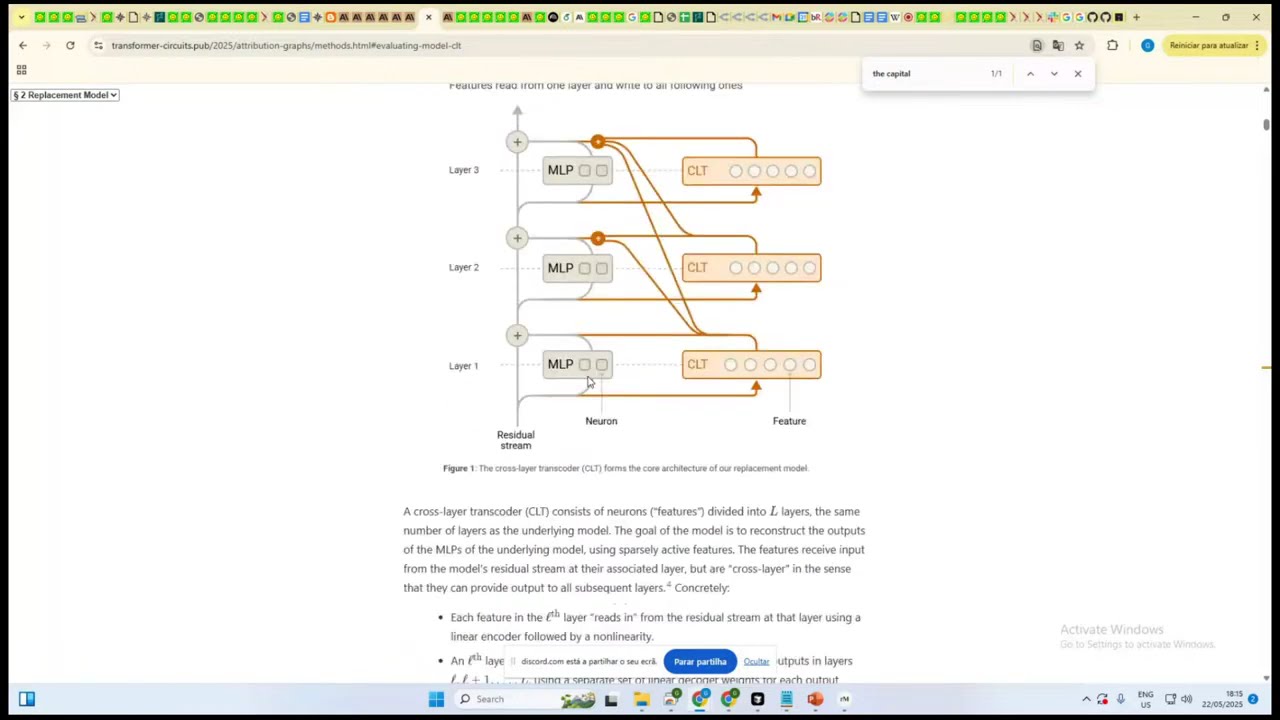
- [05:02](https://www.youtube.com/watch?v=Zi5aXGGeqgY&t=302s) Unlike standard per-layer transcoders, a single CLT reads activations from layer L via one encoder and writes predictions to layer L and subsequent downstream layers via multiple distinct decoders.
- [15:23](https://www.youtube.com/watch?v=Zi5aXGGeqgY&t=923s) Replacing MLPs with transcoders introduces prediction drift: even with massive latents, top-1 token predictions change up to 50% compared to the unperturbed base model.
- [15:23](https://www.youtube.com/watch?v=Zi5aXGGeqgY&t=923s) Despite requiring higher parameter and FLOP overhead, smaller CLTs consistently outperform larger per-layer transcoders in reconstruction and accuracy trade-offs.
- [20:55](https://www.youtube.com/watch?v=Zi5aXGGeqgY&t=1255s) Constructing computational graphs requires freezing attention patterns, inserting explicit error nodes, and computing gradient-based attribution scores backward from target output logits.
- [29:04](https://www.youtube.com/watch?v=Zi5aXGGeqgY&t=1744s) Transcoder features distinguish between input features (unconditional detectors of context strings or syntactic patterns) and output features (predictive features that promote target next-token logits).
- [27:29](https://www.youtube.com/watch?v=Zi5aXGGeqgY&t=1649s) Individual feature nodes are merged into higher-level 'supernodes' to simplify attribution graphs for human interpretation, though this abstraction can mask underlying activation messiness and edge cases.
- [31:30](https://www.youtube.com/watch?v=Zi5aXGGeqgY&t=1890s) Features frequently co-activate on the same token despite L0/L1 sparsity penalties, demonstrating that models rely on combinatorial representations rather than isolated mono-semantic units.
- [34:09](https://www.youtube.com/watch?v=Zi5aXGGeqgY&t=2049s) Node ablation experiments functionally validate graph structure by demonstrating that zeroing or suppressing specific feature nodes systematically suppresses predicted target logits.
- [34:09](https://www.youtube.com/watch?v=Zi5aXGGeqgY&t=2049s) Interventions on features at later layers produce no behavioral change if downstream components have already consumed the signal in earlier layers.
- [43:25](https://www.youtube.com/watch?v=Zi5aXGGeqgY&t=2605s) In addition tasks, CLT features organize into distinct mathematical primitives, such as exact diagonal sum bands, value range detectors, and periodic modulo strides.
- [43:25](https://www.youtube.com/watch?v=Zi5aXGGeqgY&t=2605s) Mathematical features exhibit off-diagonal polysemantic noise and activate in non-math contexts because underlying model parameters are shared with general text and code tasks.
- [01:00:44](https://www.youtube.com/watch?v=Zi5aXGGeqgY&t=3644s) Attribution graphs are highly prompt-dependent and brittle, highlighting a fundamental challenge in mechanistic interpretability regarding whether universal, prompt-invariant circuits exist.
- [01:05:36](https://www.youtube.com/watch?v=Zi5aXGGeqgY&t=3936s) The primary bottleneck for open-source circuit tracing is not the graph attribution algorithm, but access to high-quality, pre-trained cross-layer transcoders.
## Detailed walkthrough
### [00:03](https://www.youtube.com/watch?v=Zi5aXGGeqgY&t=3s) Introductory Housekeeping and Major News on Transcoders
The session opens with some brief administrative setup as the speaker checks their screen and audio feeds, noting they only have a single monitor so they won't be actively tracking the text chat. After a short musical intro pause, they share an exciting piece of industry news with the reading group and future recording viewers: Anthropic is planning an official open-source implementation release. Multiple groups are preparing to release open-source models featuring both standard transcoders and cross-layer transcoders (CLTs) soon. Additionally, there appears to be a Neuropedia-like plugin or interactive platform in development, allowing researchers to explore and play with these open models directly.
[01:49](https://www.youtube.com/watch?v=Zi5aXGGeqgY&t=109s) Core Concepts: Circuit Tracing and Cross-Layer Transcoders
Transitioning into the core presentation, the speaker recaps the central theme from Anthropic’s recent research paper (*Circuit Tracing: Revealing Computational Graphs in Language Models*): using **cross-layer transcoders (CLTs)** to perform automated circuit tracing inside large language models. The speaker connects this method to earlier mechanic interpretability techniques—such as work by St. Marks or researchers mentored by Neel Nanda—where Sparse Autoencoders (SAEs) were trained on residual streams, attention outputs, or MLP layers to discover circuits.
However, Anthropic's approach introduces key departures:
* **Linearization via Transcoders:** Instead of placing SAEs on residual streams or attention outputs, they directly replace the MLP blocks with transcoders and freeze certain elements to linearize the network.
* **Smaller, More Interpretable Graphs:** Feature attribution across transcoders yields significantly smaller graphs with far fewer nodes than traditional neuron-level circuit tracing, all while preserving model performance far better.
* **Cross-Layer Architecture:** The major architectural novelty is that CLTs don't just output to their own layer; a single transcoder encoder reads from an MLP's input at layer $L$ and uses multiple separate decoders to write to layer $L$ as well as subsequent layers.
[05:02](https://www.youtube.com/watch?v=Zi5aXGGeqgY&t=302s) How Cross-Layer Transcoders Work & The Sparsity Loss Discussion
The speaker walks through a visual diagram of the CLT architecture. In a standard model, each layer contains an MLP. A traditional transcoder reads from the input of an MLP at layer $L$ and writes to its output. In contrast, a CLT reads its input from layer $L$ via a single encoder, but maintains **distinct decoders** for every layer from $L$ onward. For example, a layer 1 CLT can write predictions to layer 1, layer 2, and layer 3 simultaneously. The overall output $Y_L$ of the MLP at layer $L$ is modeled as the sum of activations from all previous layers multiplied by their respective layer-specific decoders.
```
┌────────────────────────┐
│ CLT Encoder at Layer L │
└───────────┬────────────┘
│ (Acts via JumpReLU)
┌──────────────────────┼──────────────────────┐
▼ ▼ ▼
┌──────────────┐ ┌──────────────┐ ┌──────────────┐
│ Decoder L │ │ Decoder L+1 │ │ Decoder L+2 │
└──────┬───────┘ └──────┬───────┘ └──────┬───────┘
▼ ▼ ▼
Writes to MLP L Writes to MLP L+1 Writes to MLP L+2
```
This leads to a lively technical discussion between the speaker and group participants regarding training objectives, activation functions, and the specific sparsity penalty:
* **JumpReLU & Reconstruction:** JumpReLU is used to select active features. Transcoder weights receive gradient signals from the reconstruction losses of all downstream layers they write to.
* **The Tanh Sparsity Penalty Intuition:** A participant brings up Anthropic's use of a $\tanh$-based penalty instead of a traditional $L_1$ penalty. They explain the intuition: an ideal sparsity constraint is $L_0$ (counting non-zero activations), but $L_0$ is non-differentiable. While $L_1$ penalizes large activation values continuously, $\tanh$ acts as a smooth step function—acting like a binary switch that stays close to 1 for large positive values and 0 for near-zero values.
* **Cross-Layer Sparsity Summation:** The speaker notes an interesting detail: Anthropic calculates the sparsity penalty across all layers concatenated together (or running a joint top-$K$ constraint), forcing the entire model to optimize its total active latent count holistically rather than layer-by-layer in isolation.
[15:23](https://www.youtube.com/watch?v=Zi5aXGGeqgY&t=923s) Evaluating Model Performance & Reconstruction Trade-offs
The speaker turns to the trade-offs of replacing native MLPs with CLTs. While replacing MLPs with sparse transcoders theoretically allows clean computational tracing, reconstruction is never 100% loss-free.
Analyzing performance plots from the paper (comparing KL divergence and top-1 token prediction accuracy across cross-layer transcoders, per-layer transcoders, and thresholded native neurons), the speaker highlights several key takeaways:
* **Prediction Drift:** Even with massive CLTs containing 10 million total latents, substituting MLPs with transcoders results in the top-1 predicted token changing up to 50% of the time compared to the unperturbed base model across standard evaluation distributions.
* **CLTs vs. Per-Layer Transcoders:** CLTs consistently outperform standard per-layer transcoders. A smaller CLT (e.g., 300k features) often matches or exceeds the performance of much larger per-layer transcoders.
* **Thresholded Neurons Fall Short:** Attempting to build circuits by simply thresholding native model neurons to a comparable active count (e.g., $L_0 \approx 10,000$) yields a drastically higher error rate. Transcoders and CLTs achieve vastly superior fidelity at equivalent sparsity levels.
* **Parameter & Compute Overhead:** CLTs require more total decoder parameters—roughly $\frac{N_{layers}}{2}$ times more decoder parameters and FLOPs during training. However, because smaller CLTs outperform larger per-layer models, researchers can strike a favorable trade-off in overall network scale.
[20:55](https://www.youtube.com/watch?v=Zi5aXGGeqgY&t=1255s) Generating Computational Graphs via Attribution & Gradient Tracing
Once a model's MLPs are replaced with trained cross-layer transcoders, the speaker explains the procedural pipeline for generating a computational circuit graph for a specific prompt:
1. **Forward Pass & Caching:** Run a fixed prompt through the base model. Cache all attention pattern matrices, normalization denominators (from LayerNorm/RMSNorm), feature activation patterns across all CLT layers, and the residual error vectors between true MLP outputs and CLT reconstructions.
2. **Linearization:** Freeze attention pattern matrices and insert explicitly tracked "error nodes" into the computational stream. This linearizes the network.
3. **Gradient-Based Feature Attribution:** Perform backward attribution starting from candidate target output logits back through active CLT features down to the original token inputs. Because attention is fixed and error terms are captured as explicit offsets, direct feature-to-feature and feature-to-output contribution scores can be computed directly via gradients.
4. **Graph Pruning:** The resulting massive gradient graph is pruned by thresholding small edge weights, leaving a compact, interpretable DAG (Directed Acyclic Graph) showing the flow of information across token positions and layers.
<ElicitationsGroup message="Explore related concepts in Mechanistic Interpretability:">
<Elicitation label="Learn about JumpReLU and activation functions in SAEs" query="Explain how JumpReLU works in Sparse Autoencoders and how it compares to Top-K or L1 penalties."/>
<Elicitation label="Understand circuit tracing and attribution methods" query="How does gradient-based feature attribution work when constructing computational graphs in language models?"/>
</ElicitationsGroup>
[024:36] Tracing Latents and Attribution Graphs
The speaker walks through the scale of active latents within cross-layer transcoders (CLTs) across model layers. While there are typically around 888 tokens per layer, the number of active latents per layer fluctuates due to the jump ReLU activation function. Across all layers combined, roughly 100 to 200 latents are active for a given token. However, not all of these active latents contribute equally to the model's final output—in this specific demonstration, predicting the acronym "DAG". By tracing gradients backward from the final output token, researchers can isolate the specific computational nodes that matter most, revealing a sparse computational graph distributed across the sequence.
Most nodes in this attribution graph correspond to features activating on the target token `n`, though some activate on earlier context tokens like `digital`. Each feature node is assigned a human-interpretable label—such as `say G`, `say DA`, or `say DAG`—which were created by manually inspecting the top activating text examples and output logits. For example, a feature labeled `digital` simply fires on the literal string "digital", whereas features labeled with `say D` promote top logits that begin with the letter "D".
- **Active Latent Count:** Approximately 100–200 active latents in total across all layers for a given token.
- **Node Distribution:** Mostly centered on the current activating token, with selective context nodes on prior tokens.
- **Feature Tagging:** Node labels are manually assigned based on activating text patterns and logit distributions.
---
[027:29] Coalescing Features into Supergroups and Interventional Testing
To make these complex, highly node-dense attribution graphs readable, researchers consolidate related features into high-level "supergroups." For example, multiple individual features that all promote words starting with "D" or activate on context preceding a "D" are merged into a single "D features" supernode. This abstraction drastically simplifies the visual graph while preserving the overarching flow of information. The presenter notes a minor UI frustration during the live demonstration ("Man, why are browsers like this?") before explaining how these graph structures can be validated experimentally through causal interventions.
In theory, if an attribution graph faithfully represents the model's internal reasoning, ablating or modifying specific nodes should directly alter the final prediction. Although node-killing functionality is disabled in the live web interface being shown, the presenter explains that setting a node's activation to zero—or artificially amplifying it by a scaling factor—tests whether the sub-graph is functionally necessary or sufficient for the target output.
- **Supernodes:** Abstract clusters that merge multiple lower-level features sharing similar input or output semantics.
- **Causal Validation:** Graph fidelity is verified by zeroing out or scaling node activations and observing changes in output probabilities.
---
[029:04] Input Features vs. Output Features
The discussion shifts to distinguishing between input-side features and output-side features within the transcoders. "Input features" fire reliably whenever a specific token or pattern appears in the context, regardless of what precedes or follows it—such as a feature firing strictly on the word "digital", or a broader input feature that activates on any number ending in the digit `6`. These features encode historical context rather than directly predicting upcoming text.
Conversely, "output features" fire on current tokens to actively promote a specific next-token prediction. The presenter highlights a clear example: when looking strictly at the highlighted purple context tokens, the input pattern appears noisy and obscure; however, examining the model's top next-token prediction reveals that it consistently predicts "DAG" (or related tokens like "dog" or "wag" lower down the distribution). Other output features act at a broader semantic level—such as promoting a cluster of sports-related tokens including "football" and "netball".
- **Input Features:** Unconditional feature detectors for specific context strings (e.g., "digital") or syntactic patterns (e.g., numbers ending in 6).
- **Output Features:** Predictive features whose primary role is to drive up logits for target next-tokens or semantic categories (e.g., sports terms).
---
[031:30] Feature Co-Activation and Supernode Imperfections
A key insight highlighted by the authors is that related features frequently co-activate on the same token. Under standard sparse autoencoder (SAE) training dynamics, sparsity penalties theoretically encourage features to remain orthogonal and mutually exclusive so that a single feature handles a concept without incurring extra $L_0$ loss. However, empirical graphs show clear co-activation: for instance, four distinct features fire simultaneously on terms related to "analytics", four fire together on "digital", and up to five output features co-activate within a single group.
The presenter cautions that human-assigned supernode labels give the impression of an exceptionally clean graph, masking underlying messiness. Examining individual feature activations reveals edge cases—for instance, a feature labeled `say D` might fire two tokens after an initial trigger without activating on intermediate letters like "G", "C", or "M". Thus, while supernode abstractions make the computational graph human-interpretable, the underlying feature behaviors retain a degree of abstraction and noise.
- **Co-activation:** Multiple features routinely fire in parallel for the same input concept despite $L_0$ sparsity penalties.
- **Manual Abstraction:** Supernodes clean up visual graphs, but individual component features exhibit messier, less exact activation patterns.
---
[034:09] Node Ablation and Layer-Specific Steering Experiments
The group examines specific intervention experiments on the "National Digital Analytics Group" prompt, where the model's task is to predict the acronym "DAG". When researchers selectively suppress or "kill" the `group` feature, the dependent `say G` feature fails to activate, shifting the model's output away from "DAG" to alternative completions. Systematic ablation across different nodes reveals clear functional dependencies:
- **Killing `digital`:** Severely suppresses all downstream `say D` features and completely destroys the top-rank prediction for "DAG".
- **Killing `analytics`:** Leaves the `say D` pathway partially intact but wipes out all `say A` features, destroying the "DAG" completion.
- **Killing `say D`:** Weakens adjacent sub-nodes like `VI`, but surprisingly leaves the final "DAG" logit near baseline levels because parallel redundant pathways compensate.
The conversation touches on layer-wise feature distribution. Supernodes often contain constituent features spread across multiple layers (e.g., layer 10, 11, and 12). A participant named Gonzalo notes that steering or intervening at later layers (e.g., layer 13) has zero effect if the underlying CLT feature completed its computation at layer 12. Once downstream features have already consumed the signal, late-stage interventions cannot retroactively alter the computation.
- **`digital` Ablation:** Collapses all `D`-related nodes and eliminates the target logit.
- **`analytics` Ablation:** Selectively disables `A`-related nodes while preserving `D`-nodes.
- **`say D` Resilience:** Targeted ablation of a single `say D` node does not ruin the final "DAG" prediction due to path redundancy.
- **Layer Dynamics:** Interventions applied after a feature's final layer of influence produce no behavioral change.
---
[039:54] Cross-Layer Transcoder (CLT) Ablations and Graph Metrics
The speaker briefly highlights another case study involving the prompt "Michael Jordan plays the sport of...", where the base model surprisingly assigns only ~60% probability to "basketball", distributing the remaining probability across multiple other tokens. The conversation then turns to the architectural advantages of Cross-Layer Transcoders (CLTs) over standard pre-layer transcoders or individual SAEs.
CLTs achieve superior reconstruction loss at smaller $L_0$ sparsity values. To evaluate feature interpretability, the authors utilize automated metrics such as "sort" and "contrastive" evaluations. Additionally, CLTs produce shorter computational paths that capture a higher fraction of total influence between embedding nodes and output logits. The "replacement score" measures how much information flows from inputs to logits when keeping a minimal set of graph nodes; CLTs maximize this fidelity metric while using significantly fewer nodes than traditional sub-graphs.
- **Output Certainty:** In the Michael Jordan benchmark, the model predicts "basketball" with only ~60% confidence.
- **CLT Efficiency:** Delivers lower reconstruction loss at lower $L_0$ sparsity compared to standard transcoders.
- **Replacement Score:** Quantifies the proportion of information preserved between embeddings and logits using a pruned set of graph nodes.
---
[043:25] Case Study: Modular Arithmetic and Addition Circuits
The discussion transitions to a detailed case study on toy addition circuits, analyzing how CLT features represent mathematical operations. Instead of evaluating full attribution graphs, this experiment tracks feature activation maps when the model processes an equals sign (`=`) following an addition expression $X + Y$. Plotting feature activations across a grid of inputs ($X$ from 1–99, $Y$ from 1–99) reveals distinct functional patterns:
1. **Range Features:** Features that fire strongly on sum ranges (e.g., activating heavily when the answer falls between 50 and 60).
2. **Modulo Features:** Features whose decoder directions align with specific modular arithmetic properties—such as lighting up exclusively on numbers where $\text{sum} \equiv 5 \pmod{10}$.
3. **Exact Value/Diagonal Features:** Features that fire along sharp diagonal bands where $X + Y = K$ (e.g., exactly summing to 92 or 95).
4. **Lookup Table Features:** Conditional grid patterns that fire strictly when both $X$ and $Y$ satisfy specific discrete constraints simultaneously.
```
Y (1-99)
^
99 |........ /
|....... / <-- Diagonal Activation Band
|...... / (Sum X + Y = 95)
|..... /..
1 |.... /...
+-------------------> X (1-99)
1 99
```
A participant notes that while these visual activation grids clearly display mathematical structures (diagonals, grids, and modular strides), they also contain noticeable noise and off-diagonal "spurious" activations. For example, a feature detecting a sum of 95 might show unexpected strong activations in the upper-right corner ($X, Y \approx 90$). The group discusses why this occurs: language models do not train exclusively on pure arithmetic. Because the underlying parameters are shared across general text processing, code execution, and other reasoning tasks, arithmetic feature representations retain non-ideal side effects and overlapping functional roles.
- **Activation Grids:** Evaluated at the `=` token across a $99 \times 99$ input grid for $X + Y$.
- **Circuit Primitives:** Features split into sum ranges, exact sum diagonals ($X+Y=95$), periodic modulo strides ($\pmod 5$), and lookup grids.
- **Polysemantic Noise:** Off-diagonal activations occur because the same model weights must simultaneously support non-arithmetic tasks like natural language and code.
[50:08](https://www.youtube.com/watch?v=Zi5aXGGeqgY&t=3008s) Contextual Polysemanticity and Model "Intention" in Addition Circuits
The discussion opens with a close examination of an addition example in Anthropic's "Circuit Tracing" paper, specifically looking at how a "sum 92" feature behaves. A participant points out that when the model evaluates an equals sign after an expression like `36 + 59`, it naturally tries to sum those numbers. However, looking at the feature activations reveals that it lights up across spaces and tokens where no summation is happening at all. This suggests that the feature is doing something far broader than merely adding two specific numbers, or else the model is somehow "confused" into believing it must sum values in non-math contexts—a rather strange interpretation.
```
Prompt: "36 + 59 ="
Expected Action: Sum numbers -> Output 95
Observed Feature Behavior:
┌──────────────────────────────────────────────────────────┐
│ "Sum 92" / "Sum 95" features activate on whitespace and │
│ non-math tokens where no addition is taking place. │
└──────────────────────────────────────────────────────────┘
```
Another contributor defends the model's performance, suggesting that since it consistently outputs correct answers for two-digit addition, it deserves credit for performing a form of distributed computation or constructive interference. The conversation then turns to philosophy and methodology: how can researchers distinguish whether a model is executing a task intentionally versus experiencing accidental feature interference? A participant admits that the mechanistic interpretability community is not even close to answering whether language models possess "intentions" in what they implement. Nevertheless, in a constrained arithmetic context where the model consistently arrives at the right answer, considering it as "trying" to output the correct sum remains a useful frame.
- When inspecting SAE (Sparse Autoencoder) features in context, features that label specific mathematical outcomes (e.g., "sum 92") frequently fire on unrelated background tokens.
- The group debates whether this represents "interference" or an essential mechanism of distributed, constructive representation that enables downstream accuracy.
- "For me, the answer is that you don't know—at least we are not even close to being able to answer that question."
---
[54:37](https://www.youtube.com/watch?v=Zi5aXGGeqgY&t=3277s) Feature Ablation and Intervention Experiments
The speaker moves on to discuss feature intervention experiments, highlighting them as one of the coolest demonstrations in the paper. By artificially suppressing or disabling specific feature nodes, researchers can observe how information flows through the transformer and directly corrupt its outputs. Even if the current dictionary decomposition does not capture the true, ultimate "ontology" of the model, these interventions prove that attribution graphs provide a highly functional approximation of information pathways.
```
┌─────────────────────────────────┐
│ Prompt: "36 + 59 =" (Ans: 95) │
└────────────────┬────────────────┘
│
┌─────────────────────┴─────────────────────┐
▼ ▼
[ Suppress "Sum 95" Node ] [ Perturb Inputs / Sub-terms ]
│ │
▼ ▼
Predicts every number EXCEPT 95 Outputs 95 at wrong position, or
(spreads logit weight to 5, 15, etc.) smears probability toward 90.
```
When the model processes `36 + 59`, it naturally predicts `95`. However, suppressing the "sum 95" node causes the model to predict almost any number *except* `95`—distributing its probability across alternatives like `5` or `15`. Similarly, modifying the input inputs to `36 + 50` or `59 + 30` produces subtle failures: the model might still compute `95` but place it at the wrong sequence position, or smear its prediction probability toward `90` due to neighboring feature activations like "sum close to 92."
- Disabling feature nodes confirms that feature graphs capture real causal pathways of information flow.
- Suppressing the correct sum node eliminates the correct answer from the top logits, causing the model to output erroneous fallback numbers.
- Perturbing terms in addition prompts causes logit "smearing" and spatial displacement of the generated digits.
---
[57:27](https://www.youtube.com/watch?v=Zi5aXGGeqgY&t=3447s) The Mystery of Supernodes and Feature Superposition
A participant shifts the conversation to the phenomenon of "supernodes"—clusters of features that fire simultaneously or across related contexts—and asks why the model doesn't simply merge them during training. If redundant nodes activate at the same time in the same layer on the same token, the dictionary learning penalty should disfavor them. The group examines why these redundant groupings persist despite the L1 or sparsity penalties designed to eliminate them.
```
Layer L Token T: [Feature A (Letter 'D')] ──┐
├──> Co-activate as a "Supernode"
Layer L Token T: [Feature B (Uppercase)] ──┘
* Why aren't they merged by training penalties?
- Intersecting meanings across non-math / alternative contexts.
- Token superposition & Layer superposition.
```
The speaker explains that supernodes occur across several dimensions:
1. **Layer Superposition:** The same conceptual feature manifests across multiple adjacent layers on the same token.
2. **Token Superposition:** Related features spread across different tokens in the prompt (e.g., one node firing on a lowercase `n` and another on an uppercase letter).
3. **Contextual Combinatorics:** A feature that appears redundant in an addition context may serve a completely distinct function in another context (e.g., processing French text or calendar dates).
Because the model relies on the *combination* of active features—both upstream and downstream—to determine final behavior, sparse autoencoders struggle to find a perfectly clean 1-to-1 decomposition.
- Supernodes represent groups of co-activating features that persist despite sparsity penalties.
- Features co-activate because language models rely on combinatorial feature interactions rather than isolated, mono-semantic units.
- A single node can participate in arithmetic circuits in one context and entirely unrelated tasks (like grammar or date parsing) in another.
---
[01:00:44](https://www.youtube.com/watch?v=Zi5aXGGeqgY&t=3644s) Regularization Limits, Circuit Brittleness, and Universal Graphs
The group debates whether adding regularization penalties—such as penalizing mutual information or enforcing orthogonality between features—could eliminate feature co-activation. The speaker points out that prior attempts at forcing feature independence typically harm the SAE's reconstruction loss. Because underlying concepts in natural language are inherently correlated, forcing artificial orthogonality prevents the autoencoder from accurately reconstructing the original model activations.
"Circuits are just... you can only trace the information flow, but there's not a general, like, unique circuit for any behavior. And that's a bit sad."
This brings the discussion to a major philosophical hurdle in mechanistic interpretability: the apparent **brittleness** of attribution graphs. Anthropic’s paper focuses on single-prompt case studies rather than averaging circuits across large datasets, precisely because general, universal circuits across varied prompts may not actually exist. The current framework of transcoders and SAEs might either be an imperfect approximation with high reconstruction loss, or indicative of a reality where neural networks do not form clean, reusable computational subgraphs.
- Forcing feature independence through orthogonality penalties worsens reconstruction loss because real-world concepts are naturally correlated.
- Attribution graphs appear highly prompt-dependent; universal circuits that generalize seamlessly across arbitrary prompts remain elusive.
- Current limitations may stem from transcoder quality, imperfect L1/sparsity loss formulations, or fundamental limits of linear feature decomposition.
---
[01:05:36](https://www.youtube.com/watch?v=Zi5aXGGeqgY&t=3936s) Open-Source Replications and Community Tooling
As the session wraps up, a participant asks if any open-source replications of Anthropic’s circuit tracing work are available. The speaker shares that their team already has working internal code capable of generating and visualizing attribution graphs matching the figures in Anthropic's paper. However, running these tools requires local model access alongside trained cross-layer transcoders or cross-layer SAEs (CLTs), which are not yet widely released to the public.
The speaker notes that researchers and Anthropic fellows are actively working on public, open-source implementations expected to drop in the near future. While the mathematical logic for graph attribution is relatively straightforward to implement, the primary bottleneck continues to be training high-quality transcoders and SAEs at scale. The session concludes with warm goodbyes as the host stops the recording.
- Internal open-source implementations can already generate and render circuit tracing graphs similar to Anthropic's public artifacts.
- The main barrier to public release is not the attribution algorithm itself, but the availability of open-source, high-quality transcoders and CLTs.
- Open-source replications from Anthropic fellows and independent researchers are expected to be released shortly for community experimentation.
## Notable quotes
> [27:29](https://www.youtube.com/watch?v=Zi5aXGGeqgY&t=1649s) Man, why are browsers like this?
> [39:54](https://www.youtube.com/watch?v=Zi5aXGGeqgY&t=2394s) Michael Jordan plays the sport of...
> [50:08](https://www.youtube.com/watch?v=Zi5aXGGeqgY&t=3008s) For me, the answer is that you don't know—at least we are not even close to being able to answer that question.
> [01:00:44](https://www.youtube.com/watch?v=Zi5aXGGeqgY&t=3644s) Circuits are just... you can only trace the information flow, but there's not a general, like, unique circuit for any behavior. And that's a bit sad.
## Mentioned
Circuit Tracing: Revealing Computational Graphs in Language Models, Anthropic, Mech Interp Discord Server Recordings, YouTube, Neuropedia, St. Marks, Neel Nanda, Sparse Autoencoders, SAE, Cross-Layer Transcoders, CLTs, JumpReLU, Gonzalo, Michael Jordan
Anthropic's research on circuit tracing replaces language model MLP blocks with cross-layer transcoders to isolate compact, linearized computational graphs. While this architecture improves reconstruction and enables causal feature interventions, the resulting circuits remain prompt-dependent and exhibit noticeable feature polysemanticity and prediction drift.
Architecture and Sparsity in Cross-Layer Transcoders (5:02)
Anthropic's approach departs from standard Sparse Autoencoders (SAEs) on residual streams by directly substituting MLP blocks with cross-layer transcoders (CLTs). A CLT reads from an MLP's input at layer L using a single encoder with JumpReLU activations, but employs separate decoders to write directly to layer L as well as subsequent layers. The output at any given layer is modeled as the sum of activations from all preceding layers multiplied by their respective layer-specific decoders.
To constrain latent activations without relying on a non-differentiable L0 metric, training utilizes a tanh-based sparsity penalty. Unlike an L1 penalty that continually penalizes larger activation magnitudes, the tanh function serves as a smooth step function that stays near 1 for large positive values and near 0 for minimal activations. The speaker notes that Anthropic calculates this sparsity penalty across all layers combined, compelling the model to optimize its total active latent budget across the network rather than layer by layer.
Performance Trade-offs and Linearized Graph Extraction (20:55)
Replacing native MLPs with CLTs involves trade-offs between interpretability and fidelity. The presenter highlights that substituting MLPs with transcoders alters the top-1 predicted token up to 50% of the time relative to the base model, even in setups with 10 million total latents. Nevertheless, CLTs consistently outperform standard per-layer transcoders and drastically surpass thresholded native neurons at equivalent sparsity levels, despite requiring roughly N_layers / 2 more decoder parameters and training FLOPs.
To map computational circuits for a prompt, researchers linearize the model by freezing attention pattern matrices and LayerNorm denominators while inserting explicit error nodes to account for residual reconstruction loss. Gradients are traced backward from target output logits through active CLT features to the input tokens. Thresholding small edge weights prunes this graph into a compact Directed Acyclic Graph (DAG) that visualizes information flow across token positions and layers.
Latent Attribution, Supernodes, and Causal Validation
Tracing reveals approximately 100 to 200 active latents per token across all model layers. These latents divide into input features, which detect fixed contextual strings or syntactic patterns, and output features, which actively promote specific downstream tokens. Because multiple related features co-activate on the same token despite sparsity penalties, researchers aggregate them into human-labeled 'supernodes' (such as grouping multiple 'say D' features together) to make complex graphs readable.
Causal interventions experimentally validate the functionality of these graphs. In a demonstration predicting the acronym 'DAG' from 'National Digital Analytics Group', zeroing the 'digital' node suppresses downstream 'say D' features and destroys the top prediction. In contrast, ablating a single 'say D' feature leaves the final prediction intact due to parallel redundant paths. A participant, Gonzalo, points out that steering must respect network depth: intervening at layer 13 has zero effect if the underlying CLT feature finished its computation at layer 12.
Polysemantic Noise and Circuit Brittleness (60:44)
Case studies on two-digit addition reveal distinct arithmetic sub-circuits, including sum ranges, exact sum diagonals, and modular arithmetic strides. However, features like 'sum 92' frequently activate on whitespace and unrelated tokens. Group participants debate whether this reflects interference or constructive distributed representation, noting that mechanistic interpretability cannot currently determine whether models possess genuine computational 'intention'.
A critical limitation highlighted in the discussion is the brittleness of these computational graphs. Enforcing feature independence via orthogonality penalties harms reconstruction fidelity because natural language concepts correlate naturally. Furthermore, attribution graphs appear highly prompt-specific, and the speaker observes that universal, reusable circuits across varied prompts remain elusive.
While open-source tooling for graph attribution and visualization is already being implemented internally, public experimentation remains constrained by the computational challenge of training high-quality cross-layer transcoders at scale. Fundamental questions remain unresolved regarding whether current circuit tracing reflects an imperfect linear approximation or a deeper reality in which language models do not organize into clean, universal subgraphs.
[27:29] Man, why are browsers like this?
[39:54] Michael Jordan plays the sport of...
[50:08] For me, the answer is that you don't know—at least we are not even close to being able to answer that question.
[60:44] Circuits are just... you can only trace the information flow, but there's not a general, like, unique circuit for any behavior. And that's a bit sad.
Original transcript
[0:03] If
[0:04] people I think it should work now.
[0:09] If people want to ask any
[0:13] question they I'm I don't I only have
[0:16] one one screen so I I'm I'm not going to
[0:18] be looking at the chat. Uh but they
[0:22] can read or or that. Sure. Yeah.
[0:28] [Music]
[0:30] Let me check first that is
[0:46] working. Yeah, for for the people in the
[0:48] reading group and the almost nobody
[0:51] people that are going to watch the the
[0:54] recording. Um, yeah, you you got
[0:58] the the snoop that the scoop that uh
[1:03] yeah, there's going to be like kind of
[1:06] an official implementation from Entropic
[1:09] that's open source. A bunch of different
[1:12] people are
[1:13] releasing it both transcoders and um
[1:18] cross layer transcoders as well
[1:21] soon. And so that's that's going to be
[1:23] nice for people for people to be able to
[1:26] to use them. Um, and and there's going
[1:29] to be like an I think like a neuronedia
[1:33] kind of plugin for people to play with
[1:36] them as
[1:42] well. Okay. I don't think anybody
[1:44] watching the recordings here to get all
[1:46] the news.
[1:49] Okay. So I don't I don't think anybody
[1:52] else is
[1:53] coming. So I think I'm I'm going to
[1:56] start. So for for for the people that
[2:00] were not
[2:00] here last time or the ones that were
[2:05] here, you're going to listen to this
[2:07] again. Uh the
[2:09] idea that like one of the biggest ideas
[2:13] or that that Entropic is discussing on
[2:16] this most recent work
[2:20] is to use what they call cross layer
[2:24] transcoders to do circuit tracing.
[2:28] Um if if people are familiar
[2:31] uh this idea is is kind of
[2:34] similar to to something that that some
[2:39] marks have done already and and also um
[2:44] some people mentored by Neil uh where
[2:48] where you you take in in the case of St.
[2:52] marks you you take um SAE train strained
[2:56] on the residual stream on the output of
[2:59] attention and the output of the MLP and
[3:02] you make circuits with that uh the
[3:05] normal way that you make circuits I
[3:06] think uh which is very similar to to
[3:09] what entropic does here which we are
[3:12] going to to to to cover uh in the case
[3:15] of of the transcoder circuit artic uh
[3:18] paper um they they don't do uh residual
[3:23] stream essays or attention essays. They
[3:26] instead just substitute the MLP with the
[3:30] transcoder and and they they freeze
[3:35] um they freeze the model uh to to to try
[3:38] to linearize it. and we'll discuss what
[3:42] that means. But they they linearize the
[3:44] model and they just trace
[3:47] um the importance of of each feature uh
[3:51] of the transcoder to to the output uh
[3:55] making circuits. This is for for those
[3:57] familiar I think very very similar to to
[4:00] what we have already been doing uh like
[4:04] with neurons etc. And like the reason
[4:07] why maybe this is such a big deal is
[4:10] that
[4:11] uh yeah maybe maybe transcoders are a
[4:14] bit more interruptible
[4:17] uh doing this like you get graphs that
[4:19] are much smaller with much smaller with
[4:21] much less nodes than if you would do it
[4:24] with with with neurons uh while still
[4:27] recovering uh a good part of of the
[4:30] performance.
[4:32] Uh and the other the other advantage or
[4:35] the other novelty on this was really the
[4:37] introduction of of cross layer
[4:40] transcoders which seem to be able to
[4:44] reconstruct
[4:46] uh the model performance better uh while
[4:50] using uh the same amount or or a smaller
[4:53] amount of uh active features at any uh
[4:58] given time. So
[5:02] uh to start
[5:04] let's I
[5:06] already we already looking at this image
[5:09] but for those that are not familiar the
[5:11] idea of a cross layer
[5:13] transcoder is that uh you have a model
[5:17] which has some some layers uh and in
[5:20] each layer there's an MLP and at each
[5:24] layer you're substituting the MLP uh
[5:27] with a normal transcoder.
[5:30] uh that just reads from the input of the
[5:32] MLP and writes the output of the MLP but
[5:36] also for all layers after the first one
[5:40] um the previous transcoder also writes
[5:44] to that layer. Uh so in this case on
[5:47] layer two uh this MLP is
[5:51] reconstructed by its own layer uh
[5:55] transcoder but also by the previous
[5:57] layer transcoder. And uh while the the
[6:03] the activations of this CLT are
[6:08] are defined just by the in by a single
[6:11] encoder. So this CLT has an encoder.
[6:14] This CLT has an encoder. This CLT has an
[6:16] encoder and this encoder reads only from
[6:18] the MLP um input. Each CLT as a
[6:23] different decoder depending on the layer
[6:26] that it is writing on. So
[6:31] uh this CLT would read from this and
[6:34] with one decoder will read will write to
[6:36] layer one to a with a different decoder
[6:38] will write to layer two and with a
[6:39] different decoder it will write to layer
[6:41] three. Uh in the case of um of
[6:46] entropic they use jump ru to decide
[6:50] which of the features are active.
[6:54] uh and uh they train it with the normal
[6:57] uh reconstruction loss, MSE loss, but
[7:00] they also have uh a sparity penalty uh
[7:05] that tries to minimize
[7:10] um
[7:11] the the
[7:14] sum like
[7:16] basically you
[7:21] uh try to minimize the the total
[7:24] am amount of latent sorry of latent
[7:28] across all layers together. Um this
[7:32] means that you'll across the model
[7:34] you'll have a
[7:35] distribution of uh how many features are
[7:38] active per
[7:40] token.
[7:41] Um they yeah we train the transcoders in
[7:47] reconstruction like all of the
[7:48] transcoders are trained in with the
[7:50] reconstruction loss for all of the
[7:53] layers or at least the layers that are
[7:54] after that uh the layer transcodation
[7:58] right yeah so so
[8:01] the yeah the this this CLT will receive
[8:06] gradients also from this reconstruction
[8:09] and from this reconstruction because it
[8:11] it contributes to this reconstruction
[8:13] like uh the the Y L which is the the
[8:18] output of the MLP at layer L is the sum
[8:21] of the activations of all previous
[8:23] layers times the decoder uh of all
[8:26] previous layers as okay makes sense. So
[8:29] so you have yeah the reconstruction will
[8:31] have all the all the terms before the
[8:34] first one is train model to reconstruct
[8:37] all of the layers. Yes. The first one
[8:40] will output to all layers. Yes. Uh and
[8:43] and and it decides that it's going to
[8:46] write to all layers uh just by reading
[8:51] the first layer. So the the inc the
[8:54] encoder reads the first layer and it
[8:56] will write to all all layers but the
[9:00] decoders will be different. Yeah. Yeah.
[9:02] It has a bunch of decoders. Okay. Yes.
[9:05] Yes. Um and so
[9:09] Uh, um, yeah. Are you going to talk
[9:11] about the sparsity loss more? Because,
[9:16] um, I've seen L1 penalties and I thought
[9:18] this was really interesting that they
[9:21] have this tanh now. Um, I don't know if
[9:23] people started doing that and I only
[9:26] just found out.
[9:29] Uh, I think so. I think they they've
[9:32] they've done 10H sparity penalties
[9:36] before to be honest. I'm too dumb to
[9:39] understand this sparity penalty. Uh like
[9:42] I don't quite understand like I mean I I
[9:47] I I I don't have an intuition why it
[9:49] would have this shape uh or why why it
[9:52] is better. Uh if you want I have an
[9:54] intuition. Yeah, I have an intuition I
[9:57] can share. Um yeah. So, so if you have
[10:01] if you have no sparity penalty, okay,
[10:05] and you build some kind of autoenccoder
[10:08] where the dimensionality in the middle
[10:09] is higher,
[10:12] then it can get zero loss by just
[10:14] actually copying all the inputs with
[10:17] right with just an identity and then
[10:19] having zero for all the extra nodes,
[10:23] right? So what we really want it to do
[10:25] is to is to find these these these uh uh
[10:30] uh concept directions such that the
[10:34] number of nonzero
[10:36] values will be as low as possible on any
[10:41] given you know
[10:43] activation. Okay. So if the residual
[10:46] stream is you know dimension whatever
[10:48] you know 16,000 you you want fewer than
[10:51] 16,000 activations at once
[10:55] presumably. So what you really want is
[10:57] an L0 penalty.
[11:00] Yeah. Okay. But L0 is not
[11:03] differentiable. So we use an L1 penalty.
[11:06] tanh within a certain
[11:08] region imitates an L0 penalty
[11:13] because it doesn't keep going up and up
[11:15] like
[11:16] L1. It's just
[11:20] either one close to one for large
[11:24] values, right? Or 0 negative 1 whatever,
[11:27] you know, for for other values. And so
[11:30] it acts a little bit more like a
[11:32] binary penalty.
[11:36] Right. It's like a it's like a smooth
[11:40] step function. Yeah. Yeah. So I think
[11:43] that's what it is is is you want an L0
[11:45] step function but this is a a smooth
[11:47] version of it. Yeah. Sorry I I meant to
[11:51] say that so I I have intuition on why
[11:54] you want sparity. I what I meant to say
[11:56] is that I don't it's not obvious.
[11:59] uh well not it's not obvious but they
[12:02] also do this summation over the layers.
[12:06] So they're they're which I think is
[12:08] interesting. So they're not only uh
[12:13] making um each individual transcoder
[12:17] sparse but they're
[12:19] making they're constraining all of them
[12:23] to to minimize their sparsity. So
[12:27] they're trying to minimize their sparity
[12:30] together, which is which is interesting
[12:32] fact that they link they link it they
[12:34] link them together like you could have
[12:36] this you could still have this sparity
[12:39] loss. Uh well in the so in the case of
[12:43] the top K uh you can just do top K over
[12:47] each layer. Uh but in in in their case
[12:51] it's like they're doing top K across the
[12:55] layers as well. Yeah. Yeah. Or
[12:58] concatenating all together and then
[13:00] doing top. Are you familiar with the
[13:02] diagram in the October 24
[13:07] post? I found that to be really
[13:12] helpful. The top one under
[13:17] October. So if you scroll down a little
[13:20] bit, this one right there,
[13:24] uh, just up a little bit, the yeah, the
[13:27] these two that are on your screen go
[13:28] together. So they say that because of
[13:30] the residual stream,
[13:32] actually your
[13:36] your sparse features could be spread
[13:39] over different layer MLPS. Yeah. Yeah.
[13:43] And so, so down below, the one that's
[13:46] still on your screen, but below where
[13:48] you see the two of them fuse
[13:50] together, that's the L well, the the
[13:54] penalty that they're really trying to
[13:56] implement with I think the extra
[13:58] summation. Yeah. Yeah. Yeah. I think I
[14:01] think I think that that's the logic as
[14:04] well. Uh and it's interesting they don't
[14:06] discuss it here. I
[14:09] think at at least I didn't see any of
[14:12] these plots. But no, you that's why I
[14:15] was wondering if you were going to spend
[14:16] more time. I didn't see it. Yeah. Like
[14:20] uh one thing that I I I know people are
[14:22] doing is that you can look at the
[14:24] distribution of of sparity across layers
[14:27] and you'll have Yeah. You'll have
[14:29] something that's not homogeneous. uh but
[14:31] in instead um like you have a spike on
[14:35] the earlier layers and then it goes down
[14:37] and then it goes up again on the later
[14:39] layers. But but I think it's probably
[14:41] too noisy to to have any kind of meaning
[14:44] for that. But I I think it's you can
[14:46] probably maybe decompose that into
[14:49] different feature groups and and and try
[14:51] to to see like meaning of different
[14:53] parts of the the trans the the model. I
[14:56] think
[14:58] yeah I don't know that it would be worth
[15:00] taking the time to do it but I would my
[15:03] intuition is that if you have
[15:06] communication across layers that they'll
[15:08] be near each other that you're really
[15:10] never going to have layer one combining
[15:12] with layer 20 to form a feature.
[15:17] Mhm. Yeah. All right. Thank you.
[15:23] Uh yeah. So after you have this this CLT
[15:28] model,
[15:30] uh if your reconstruction loss was
[15:31] perfect, which it never is, if it was
[15:33] perfect, you could just put it instead
[15:36] of the MLP and now you have something
[15:39] that just fires very sparsely and
[15:42] hopefully all the features are
[15:43] interpretable. So you could just trace
[15:45] the computation
[15:47] uh very well. uh sadly that's not
[15:52] exactly the case and I think that this
[15:54] plot is is is a very it's a very nice uh
[15:59] way to to look at it.
[16:02] Um so here they're plotting the
[16:05] different sizes of cross layer
[16:08] transcoders per layer transcoders and
[16:11] the idea of thresholding neurons until
[16:14] you have just a certain number of
[16:16] neurons that are active and I can I can
[16:19] explain that a bit better uh later. But
[16:22] um here in this plot you see that even
[16:25] if you use a cross layer transcoder
[16:27] where in total you have 10 million
[16:30] latents
[16:32] uh when you substitute these cross layer
[16:35] transcoders uh your MLPS by these cross
[16:38] layer
[16:38] transcoders you you still get that half
[16:42] of the time uh your top prediction will
[16:45] be different from the top prediction
[16:48] prediction uh from from the base
[16:51] model. Um, and like this is just a a
[16:56] very let's say fine grained way to look
[16:58] at KL divergence, but gives you a number
[17:02] that's easier to think about. Like if if
[17:05] uh if this was like question answer uh
[17:09] if if this was measured in in a question
[17:11] answering context like this would mean
[17:14] that it would flip the answer half of
[17:17] the time. Uh which seems bad. Obviously
[17:22] uh if you probably in that context this
[17:25] fraction of incorrect would be a bit
[17:26] different. uh like here they're
[17:29] measuring this over like the full the
[17:32] full distribution like the normal
[17:33] distribution and there's much more
[17:35] options than just like four or two. Uh
[17:39] but indeed changing the top token that
[17:42] much means that the the model is is
[17:45] performing different. It's not the same
[17:47] model. You're not reconstructing
[17:49] perfectly uh the behavior. Uh and what
[17:52] this plot is showing is
[17:54] that even the smaller uh cross layer
[17:58] transcoders are competitive with the
[18:01] bigger per layer transcoders.
[18:04] Um and and they let's say it seems like
[18:08] they maybe perform a little bit better
[18:11] like the the jump from 300k to 10 to 10
[18:16] million is is wider than from 300k to 10
[18:19] million on the perance coder. And on the
[18:21] other hand here this line of
[18:25] neurons the idea is that this line I for
[18:31] me it's very weird that it actually
[18:33] doesn't go to zero but like eventually
[18:38] if you don't threshold neurons obviously
[18:41] uh you'll just have the same prediction
[18:43] of the base model but they say okay if
[18:46] you threshold it at this L0 so if if
[18:49] your neurons
[18:50] If only uh uh 10,000 neurons are active
[18:55] at any given time, they start to be
[18:57] interpretable, but you see that uh you
[19:01] get a very high uh error rate much worse
[19:04] than than transcoders. So like the
[19:06] argument could be okay maybe you can
[19:09] just do this replacement with neur with
[19:13] neurons that were thresholded uh but
[19:16] they're only interpretable after this
[19:18] thresh above this threshold and here
[19:22] there's already transcoders that are
[19:23] better and CLTs that are much better.
[19:26] This plot the KL divergence is just the
[19:28] same thing as here the scaling is a bit
[19:30] different but uh the idea is the same.
[19:34] So here they're justifying they're
[19:35] showing okay cross layer transcoders are
[19:38] worth it because they they're better
[19:40] than transcoders even though cross layer
[19:43] transcoders have more parameters than
[19:46] transcoders because even though they
[19:49] have the same number of encoder
[19:51] uh parameters they have
[19:55] um one one decoder per layer. So you you
[19:59] end up having I think they say
[20:03] uh n divided by two more decoder
[20:07] parameters right something like that.
[20:11] Um where is
[20:19] it? Yeah you have n layers divided by
[20:22] two more decoder parameters and flops.
[20:25] So, so they train
[20:28] slower. Um, but
[20:32] um
[20:34] because even smaller cross layer
[20:37] transcoders are better than than than
[20:39] bigger transcoders, you can probably
[20:42] make a tradeoff uh and and not make the
[20:45] the biggest transcoder and still end up
[20:48] with a with a better uh replacement
[20:51] model. And so now that you have a
[20:55] replacement model, uh what what do you
[20:58] do? The
[21:00] idea is that uh you substitute your
[21:04] neurons with the the active
[21:07] features and
[21:09] um you first so you first run through
[21:13] the model a fixed prompt as whatever the
[21:16] prompt is. You collect the activation
[21:19] patterns and the normalization
[21:22] uh from layer norm or whatever kind of
[21:25] norm that your model
[21:28] has and you compute the activations of
[21:32] all your feature all your layer all the
[21:35] layers of your CLT uh and compute the
[21:38] error between the true MLP and uh the
[21:43] the the the reconstructive CLT. Uh and
[21:47] so you and you store all of these. So
[21:49] you store the attention patterns, the
[21:51] normalization denominators and the
[21:53] error. Uh and now you can try to make a
[21:59] graph
[22:01] uh that uh goes only through the the
[22:06] features that are
[22:07] active. And if you freeze the attention
[22:11] and by having the the error nodes uh
[22:14] because you computed the error uh you
[22:17] are able to um to just compute the
[22:20] direct contribution uh like you can do
[22:24] attribution of how much each feature
[22:28] matters for for for the output and how
[22:32] much each feature matters for the next
[22:35] output. uh freezing attention uh is
[22:39] important. They they still use
[22:42] um they still uh compute
[22:46] um the I always forget the the OV
[22:50] circuit but they they they freeze the
[22:52] attention pattern. Um
[22:56] um I think this is yeah this is
[23:00] explained here.
[23:03] I am going to be honest, it took me a
[23:05] long time to actually understand what's
[23:09] happening here. And they have like the
[23:11] like they have an appendix that explains
[23:13] like the the exact mats. Uh but the idea
[23:18] is is that you're kind of tracing the
[23:19] gradient uh
[23:21] of you make you have a node that's your
[23:26] your output your candidate token and for
[23:30] each candidate token that you want to
[23:32] trace uh you you make all the possible
[23:35] paths through all the features uh and
[23:39] then to the
[23:41] input and and yeah you just compute
[23:44] gradients Um and and these gradients
[23:48] will tell you uh how much each of the
[23:51] nodes contributes to uh to the output.
[23:55] And I think they have Yeah. So they have
[23:58] at the end you'll get something like
[24:01] this. Does this the zooming in work?
[24:04] Yeah.
[24:18] Yeah. So at the end you have something
[24:20] like this where this is
[24:24] already this is already a a pruned
[24:27] graph. So um if if you have this is your
[24:32] input prompt which has 1 2 3 4 5 6 7
[24:36] eight eight eight tokens per token per
[24:40] layer you will have as many latents are
[24:43] active on on per layer uh which as we
[24:47] saw because it's a jump rant number but
[24:50] it's it's going to to fluctuate I think
[24:53] the the ones that they're using across
[24:56] like the sum overall all layers there's
[24:59] around 100 to 200 active latent and so
[25:04] you'll have 200 active latent per
[25:07] token but uh not all of these latent are
[25:13] as important for the final contribution
[25:18] uh which for the final output which in
[25:20] this case is is dag
[25:22] uh and by tracing the gradient so from
[25:26] this final
[25:28] from this output uh you see that there's
[25:31] all these different nodes which I'm just
[25:35] going down and these are the node that
[25:38] matter the
[25:39] most for for the output and you see that
[25:42] they're distributed all around the graph
[25:46] most of them are features that activate
[25:49] on uh the token n but some of them you
[25:54] see you will see like this one activate
[25:59] on the on the token
[26:01] digital. Uh and you'll see that each
[26:04] feature has this label. For instance,
[26:07] say G, say DA, say DAG. Uh and these
[26:12] labels are
[26:17] made, man. Why why are browsers like
[26:21] this?
[26:23] Uh and I
[26:26] already yeah these these these labels uh
[26:30] were made uh by manually looking at act
[26:36] activations. to uh this sg feature here
[26:41] you'll
[26:43] see that in in principle the idea would
[26:48] be that after
[26:51] afterwards there's there's like some
[26:53] some words that have G's you see a G I G
[26:58] I
[26:59] G G E G P LG whatever and they they made
[27:06] these these labels
[27:08] manually. Uh they say that it's
[27:12] possible. So this one is called just
[27:14] digital because it activates on digital.
[27:16] Uh some of these you you see for
[27:19] instance this say if you look at the top
[27:22] logits most of the top logits start with
[27:24] D as well. Uh and so the idea is that
[27:29] after you have this graph uh you can
[27:32] group your features. So you can have all
[27:37] your you have like one you have five
[27:40] features a D features like all of these
[27:43] uh the do logs are going to be words
[27:46] with D and all the activating examples
[27:48] are going to
[27:49] contain the D after the activating
[27:53] token. And so you can make this very
[27:56] simplified and pretty graph uh with
[27:59] which with me many less nodes uh than
[28:03] than oops than this graph because you
[28:05] just coales them into what they call
[28:08] super groups. Uh, and then the idea
[28:12] after you have these these graphs is
[28:16] that you could potentially and and this
[28:18] doesn't work in this interface, but you
[28:20] could potentially
[28:22] uh kill some of these nodes and see how
[28:26] much they the the the output changes.
[28:30] And hopefully if your graph is actually
[28:33] uh computing anything real about what
[28:36] the model is doing
[28:38] uh disconnecting these nodes or or
[28:41] changing the nodes with some other
[28:42] values uh would uh change the the
[28:47] output. Uh I think this is okay. This
[28:52] understanding and labeling features was
[28:53] what I just described.
[28:56] Um
[28:58] the I don't know if we want to read this
[29:01] but the idea one interesting idea is
[29:04] that they find
[29:06] features that are just input features um
[29:10] which is they activate on digital and no
[29:14] matter what uh comes next or before they
[29:18] just activate on on on digital and
[29:21] they're not really like
[29:23] predicting what's coming next. But maybe
[29:27] they are because obviously digital
[29:30] there's like they it only present some
[29:32] some context but it's it's mostly like
[29:34] an input feature but they also talk
[29:38] about something that's an output
[29:39] feature. So you see that all these
[29:43] activations are if you're just looking
[29:46] at the at the purple it's maybe not
[29:49] obvious what the pattern is. There's
[29:51] some mess here here. There's some A's
[29:53] here, some re here. But if you look at
[29:56] the next token, it's always dark. And so
[30:00] this would be an output feature. And in
[30:03] fact, if you look at the top uh
[30:05] predictions, it's dark dog. And then
[30:07] maybe it becomes less obvious. I don't
[30:10] know if like if we go to less activating
[30:14] examples. So now here you see in less
[30:16] activating examples there's there's Wag
[30:18] as well. But for most of the
[30:20] distribution you have you have DAG. So
[30:23] this is like an output
[30:25] feature. Uh then there's like output
[30:29] features which are not
[30:31] uh let's say as clean as the other one
[30:33] like it it just the the top predictions
[30:38] are just different types of sports. So
[30:40] it just promotes sports like
[30:44] football, netball, stuff like that.
[30:50] Um, and yeah, and this one is the same
[30:53] as an input feature. It's just that it's
[30:56] not it's not as simple as the the other
[30:59] one above, which was just a digital, but
[31:02] it it activates on all numbers that
[31:04] finish with an with a with a six. So,
[31:09] it's it's still an input feature. It's
[31:10] just that sometimes it's not input
[31:14] features are not single token. there
[31:16] they they have a pattern that's that's
[31:18] that can be uh interpretable. Um yeah,
[31:22] these are just other kinds of features
[31:24] but uh we don't really care about this.
[31:27] Uh again grouping features into super
[31:30] nodes this I think is a very interesting
[31:32] idea. I think
[31:34] people maybe when thinking about
[31:37] features
[31:40] uh like to think about them as as
[31:43] independent things especially because
[31:46] like the the whole idea of of like
[31:48] sparity is that
[31:50] um yeah that if if you have two features
[31:53] that are related
[31:55] uh it makes if if if you're training the
[31:59] model to be sparse
[32:01] uh you You' not you not not want them to
[32:05] be active on the same time because then
[32:07] your spacity is higher and so your model
[32:09] will try to specialize and make make
[32:13] features for
[32:15] for make one feature that that contains
[32:18] the two somehow. But but here we they
[32:22] they clearly show
[32:24] that for a bunch of features for
[32:28] instance here like in an analytics you
[32:30] have at least four features that are
[32:33] active at the same time on on words that
[32:36] are similar to analytics uh four
[32:38] features that are active at the same
[32:39] time on features that are similar that
[32:41] are uh input features of digital and
[32:44] even on let's say output features you
[32:47] can have more than one uh active at the
[32:49] same time in most of the groups. So you
[32:51] say in this group there's there's even
[32:53] five. Obviously these groups are not
[32:55] exhaustive. Uh and they're
[32:58] very crude in the sense that if you look
[33:02] at the let's say the
[33:04] SD feature uh like it's hard to say that
[33:09] this is actually a SAD feature. You see
[33:11] that after the most activating token,
[33:14] well, so there's the first activating
[33:16] token, then there's a a second
[33:18] activation and then D is active. But
[33:21] maybe so in this case, I don't see like
[33:24] that there's any activation on G or here
[33:27] on this C. There's no activation on on C
[33:29] or in M. So this is definitely a say D
[33:34] after a bit, but it's it's it's not
[33:37] exactly say D. This one I think is even
[33:41] clearer like there's
[33:44] idle ca. So the all are are a bit more
[33:50] abstract uh and and and and they were
[33:53] made by by a human and that's why they
[33:55] they
[33:56] look it makes it looks like the graph is
[33:59] very clean but obviously there's some
[34:01] kind of like even
[34:04] uh mess. Uh and yeah the what I was
[34:09] describing okay now you have these
[34:11] graphs how do you how do you know if
[34:15] like this is
[34:16] actually related to how the model is
[34:19] doing anything?
[34:22] Um they talk about doing
[34:25] interventions. Um so you can you can
[34:31] just do do the inter copy the the normal
[34:35] activation that the model will have
[34:38] right you think that this node is
[34:39] important on your normal pass. You you
[34:42] save this and you
[34:45] just add this feature on all the feature
[34:50] layers as it should be, but maybe you
[34:51] multiply by a certain number just to to
[34:55] make it even stronger. And for instance
[35:00] here they show that um for this DAG
[35:05] example and DAG example where the the
[35:08] model has to find the acronym for this
[35:13] national digital analytics group if they
[35:17] kill the group feature which uh because
[35:22] of that doesn't activate the SG feature
[35:27] uh it will it makes the the output
[35:30] change from from dag to just something
[35:33] that has they other them than they dag
[35:38] which this feature kind of predicts that
[35:43] that the model will say something about
[35:45] say da but now there's no reason to say
[35:48] dag uh because the the the g feature was
[35:50] was suppressed and I think they show
[35:56] here
[36:12] Uh yeah. So if you if you if you inhibit
[36:15] each of these nodes, so if you if you
[36:17] kill digital
[36:20] uh all the all the nodes that start with
[36:24] say something with D become much much
[36:28] smaller and in fact the I guess this
[36:31] logic is just the the correct answer is
[36:34] just dag. Uh it completely ruins the
[36:37] duck prediction. Uh if you kill
[36:40] analytics, you still influence a bit of
[36:42] the day but the D but uh you kill all
[36:46] the A's uh and obviously DAG and then
[36:49] the prediction.
[36:51] Instead, if you if you kill uh say
[36:56] D uh you only make
[37:00] uh the you make the VI node uh weaker.
[37:06] These ones are not connected directly.
[37:09] So they are not influenced. Uh and
[37:13] interestingly uh the the logit node even
[37:17] though the
[37:19] seda the sedag um feature is dead uh you
[37:26] still have the correct prediction. I
[37:28] think I think that's what this logic
[37:30] means that it
[37:33] doesn't that the the the fra the
[37:35] activity is still very close to
[37:39] to yeah to the
[37:41] baseline and
[37:45] um yeah some of some of these nodes uh
[37:48] some of these nodes for instance uh
[37:50] let's see if I can find you see some of
[37:53] these nodes like these super nodes like
[37:55] this say a feature like super feature
[37:58] is actually in three layers. You see
[38:02] it's here, here, and here. These two are
[38:04] on the same layer. And I think this one
[38:06] is So all of these are in different
[38:08] layers, but inside the same group, you
[38:10] have different layers. All of these are
[38:11] going to be are also in the the same
[38:14] layer. Yeah. Right. Yeah. And so one
[38:19] thing that they're saying is, okay, can
[38:21] we find
[38:22] uh what are the the layers that matter
[38:25] the most?
[38:29] Um and they just
[38:32] do they just steer in different layers.
[38:37] Uh and they see that
[38:39] um yeah there's some layers that it's
[38:42] important to steer and steering works
[38:44] and and makes the prediction wrong. Uh
[38:48] but some some features where yeah where
[38:51] if you if you just steal it later it
[38:53] doesn't uh help that
[38:56] much. Um think Gonzalo
[39:01] one other point on that is if the last
[39:04] analytics feature is on layer
[39:07] 12 that that that the CLT identified
[39:10] then when you steer on 13 of course it's
[39:12] going to have no effect because it
[39:14] already finished doing its work.
[39:18] That's a good point. Yeah. Yeah. So if
[39:21] if
[39:23] if all the inputs if all the input
[39:26] features
[39:28] uh that that receive this analytics
[39:31] feature are after your intervention
[39:34] uh they will not compute anything and so
[39:36] it your intervention is doesn't do
[39:39] anything because it it was already
[39:41] computed by by the the future
[39:45] uh features. That that's a good point
[39:47] and I think yeah this is what it kind of
[39:50] tries to demonstrate uh here. Uh this is
[39:54] a sorry this is a case study that's
[39:56] basically the same like the same thing
[39:59] uh but now instead of the d of dag it's
[40:03] it's using
[40:06] um Michael Jordan plays a sport.
[40:10] Interestingly, this model only thinks
[40:12] with certain 60% certainty that he plays
[40:18] basketball. The rest is scattered
[40:20] through multiple
[40:21] tokens.
[40:23] Um the same thing here. Uh I think
[40:28] um yeah, so there's this develation case
[40:31] study which I think we can look at. Uh,
[40:35] I don't know if people
[40:39] care about some of the CLT
[40:44] um like
[40:46] details. Uh, for instance, the fact that
[40:50] yeah, the reconstruction loss
[40:53] uh is better for for smaller L0 than the
[40:57] than the pre-layer transcoders.
[41:00] Um they also do some interpretability
[41:04] analysis
[41:05] uh where they
[41:07] show that for the same reconstruction
[41:10] loss uh you can have well for better
[41:13] reconstruction loss uh you can have more
[41:16] interpretable
[41:18] um features and by the the way that they
[41:23] measure interpretability is with this
[41:25] sort and this contrastive eval um if you
[41:30] don't know what they are,
[41:35] um they're a bit complicated to explain
[41:38] and I don't quite understand why they
[41:39] care about I think these are a bit hard
[41:42] to to reason about.
[41:46] Um but but basically what they're
[41:49] claiming is that cross layer transcoders
[41:51] are just better at reconstruction and
[41:54] better uh at being interpretable uh in
[41:57] this case by by by clog.
[42:01] Um yeah they they they also show that um
[42:05] you need
[42:06] less you can have shorter paths that
[42:09] contain
[42:11] um more influence. And I think there's a
[42:14] a new one, a different
[42:16] one. Yeah, that just shows that you can
[42:20] you can by having as a a smaller L0 um
[42:25] your your graphs are going to be more
[42:28] complete and uh more correct in the in
[42:33] this replacement score. uh which uh just
[42:36] measures the fraction
[42:40] um yeah just measures the fraction of of
[42:44] information that goes from from your
[42:46] embedding nodes to the logic nodes if
[42:49] you just kept all possible nodes
[42:52] um you'd
[42:54] have well you'd have
[42:58] uh one and one um but obviously you want
[43:02] to to have the highest number for both
[43:05] by adding the the least amount of of
[43:08] possible nodes in
[43:10] the in the graph. They also talk about
[43:13] pruning. It's I think pruning is a bit
[43:16] of a like a technical thing. If you want
[43:20] people want to read the implementation
[43:21] they they can
[43:25] um and I guess if you want we can
[43:30] try
[43:32] understand this addition case study
[43:36] um where now here they don't look
[43:42] only at
[43:45] [Music]
[43:46] um they don't look only at um at the
[43:52] graphs but they also look at um
[43:57] activations of features.
[44:01] uh for instance if I'm if I'm
[44:04] understanding this
[44:05] correctly this this
[44:07] feature
[44:09] activates on on numbers on all numbers a
[44:14] high strongly activates on all numbers
[44:16] between 50 and 60 even though it
[44:19] activates on all numbers uh more or less
[44:22] uh while this one
[44:27] uh the direct effect of the sum of a
[44:29] feature decoder on the output Yeah, in
[44:32] this one instead of being the activation
[44:33] of the feature, uh it's
[44:37] the like the logic length. So you
[44:45] you take the decoder direction of that
[44:48] feature and you see that
[44:52] uh it it lights up
[44:56] on all numbers that are five modulo 10.
[45:00] Uh I think that's how you interpret
[45:04] these
[45:05] graphs. Um so you see for instance this
[45:09] feature here
[45:12] uh you see there's all of this all of
[45:16] these activations on random
[45:18] tokens. Uh but if you just look at the
[45:22] top tokens,
[45:24] uh most of them
[45:27] are like uh numbers from from 90
[45:33] to to 99
[45:36] uh and and the bottom ones are uh 100
[45:40] which is kind of what is represented
[45:42] here.
[45:46] Um, this on the other end really makes
[45:51] it sharp that it's 99 95 like the the
[45:57] top are all
[45:59] 95. Um, this one
[46:04] uh is modules five. So this is kind of
[46:08] modules 95, but you you're only seeing
[46:12] from 0 to 100. So modules 95 just
[46:14] activates on uh 95 and and they they see
[46:19] that there's this these patterns for a
[46:21] bunch of different features. There's
[46:23] these lookup table features
[46:26] um which I don't quite understand the
[46:29] patterns. I think they show show it
[46:32] here.
[46:34] um they
[46:36] activate conditionally
[46:39] on this and this and so they activate
[46:43] only
[46:44] on when both of them are true which
[46:48] makes this these grid patterns because
[46:51] here here the numbers go from one to to
[46:53] to nine. So these are nine squares and
[46:57] the numbers go from one to nine as well.
[47:03] Uh I don't know if people have read this
[47:06] and there's anything interesting here
[47:08] that they want to discuss. I like I like
[47:11] this. I think these patterns are very
[47:13] cool. Uh but maybe I didn't explain them
[47:16] correctly. So if
[47:21] people people want to to say
[47:27] anything okay so I I was explaining
[47:30] something wrong. So they're actually
[47:32] looking at the activation on the equals
[47:35] sign of the So this is a they're looking
[47:38] at the features that are active on this
[47:41] only on this
[47:45] equal sign. And so the X here is
[47:52] the one of the one of these numbers, the
[47:56] Y is the other number. And they just run
[47:59] all possible tokens and they see the
[48:01] activations. And you see that they
[48:04] activate mostly on this diagonal which
[48:08] is going to be that the sum of these two
[48:09] numbers is close to 92. And in this case
[48:13] it's precisely 92. In this case uh it's
[48:17] modulus 5 and that's why it makes this
[48:20] pattern. In this case, it just sounds to
[48:24] be
[48:24] around it's just 40 + 50 which can make
[48:29] all these blob
[48:31] and all these shapes are the different I
[48:34] don't understand
[48:36] this. Uh this just means that doesn't
[48:39] matter what's here. It will always be uh
[48:44] 57 uh and this is the same but nine
[48:48] because it's modules. you were saying
[48:50] something.
[48:52] Yeah, I was just going to say my first
[48:54] reaction is this
[48:56] seems kind of
[48:59] inefficient and errorprone. When you
[49:02] drill in like on the sum is 95 one,
[49:07] you'll see that in the upper right
[49:08] corner there's some stronger activations
[49:10] that are nowhere near 95. um I think is
[49:14] what you scroll up. But anyway, the
[49:15] point is on all of them you'll see some
[49:17] things that are just like not really
[49:19] quite fitting the pattern. Um yeah. Uh
[49:24] but then I kind of reminded myself that
[49:28] the LLM is Oh yeah, this one you see in
[49:30] that corner there. Um and then on the
[49:32] right, the ad9 you see it's mostly a
[49:34] strong vertical pattern, but there is
[49:36] some horizontal stuff at the bottom and
[49:38] on the right, right? But then I reminded
[49:41] myself that this this model is not only
[49:46] doing addition. So maybe some of these
[49:49] other patterns that don't seem right to
[49:52] me, maybe they help with multiplication
[49:56] or fractions or something else.
[50:01] Yeah. In fact, in fact, you see that um
[50:04] like the activation of the feature that
[50:08] when it is on an equals, it tries to to
[50:14] sum like if if if if it sees 36 + 59, it
[50:19] tries to sum those numbers. But if you
[50:21] just look at this, you can see that it
[50:24] is active on a bunch of different
[50:27] features. like it's active on these
[50:29] spaces where there's not there's no sum
[50:32] here. There's no sum here. And so yeah,
[50:36] it's clearly doing something more than
[50:39] just summing 92 or at
[50:43] least otherwise the model is a bit
[50:45] confused and thinks that in this space
[50:48] somehow it must be summing something
[50:50] which is obviously a strange meaning
[50:53] thing.
[50:56] Yeah, I mean, yeah, that's right. Like
[50:58] it could be confused, but I think the
[51:01] more I thought about it, I'm going to
[51:02] give it credit for some sort of
[51:04] distributed computation, constructive
[51:06] interference, and that it's actually,
[51:09] you know, since it does get the right
[51:11] answer for all the two-digit additions,
[51:14] this is probably helpful in some way, I
[51:17] just don't understand.
[51:26] Yeah, I was wondering like how do they
[51:30] know like I think in this example it's
[51:32] pretty clear, but how do they know um
[51:37] when the model is doing something on on
[51:41] purpose versus when the model is like
[51:45] doing something or it's trying to do one
[51:47] thing but it's accidentally in some
[51:49] cases doing the other thing. like with
[51:51] the sum 95 features and that up right
[51:53] corner like is could that be
[51:56] interference like how can they tell
[51:58] between the models like or can the model
[52:00] even be said to have like intentions to
[52:03] what it's meant to implement like uh
[52:12] [Music]
[52:14] um for me the answer is that you don't
[52:18] know at least we are not even close to
[52:21] like being able to to answer that
[52:23] question. I don't know if people have
[52:26] opinion.
[52:34] I mean in this case you have the model
[52:36] and it you ask it a math question and it
[52:39] gets the correct answer. I think it
[52:41] makes perfect perfect sense to like
[52:43] consider that it's in some sense it's
[52:48] trying to output the correct number to
[52:50] the math question because was trying to
[52:51] out the correct number of the math
[52:53] question.
[52:56] Yeah. So I
[52:58] definitely Yeah, I think that's a valid
[53:00] question. I in in the in
[53:03] the like thinking about is this actually
[53:07] a sub 92
[53:09] feature something like that it it
[53:12] becomes clear clear or or clearer that
[53:17] in this specific context where you're
[53:20] doing sums it is probably a sum 92
[53:23] feature but it's still probably doing m
[53:26] much more things
[53:28] uh and and and there's like we still
[53:30] haven't found like the clean the
[53:33] composition that people have been
[53:35] waiting especially with like ses
[53:39] um because in different contexts it
[53:41] seems to be doing something else like
[53:44] maybe yeah maybe if you if you're doing
[53:47] this task of speaking French uh with
[53:50] some numbers uh you'd find a different
[53:53] circuit that would be very clear what it
[53:56] is doing even though it it it's weird
[54:00] that it would be that because obviously
[54:02] the top logits are are numbers but maybe
[54:05] maybe it's doing something about dates
[54:07] or whatever. Uh but if this is the real
[54:10] ontology of the model uh I think I think
[54:15] it's very hard to to say
[54:21] something. I don't know if that if that
[54:24] was kind of your question or not.
[54:28] Yeah, I think that was a pretty good
[54:29] response. I think I think it's just
[54:31] hard. Yeah.
[54:33] Yeah. Yeah. So, so we are already at
[54:37] seven. Um, the rest is more uh So, this
[54:41] is a cool thing I think as well. So, you
[54:43] can Yeah. you can just disable some of
[54:46] the of the feature nodes and this
[54:49] impacts like future things like
[54:52] obviously if the model doesn't know that
[54:54] it's adding stuff then it cannot know
[54:56] that the sum is a certain value. Um
[55:00] so even if this is not the correct
[55:03] ontology or something it is definitely
[55:07] like a an approximation of the pathway
[55:11] of information going through uh the
[55:14] model and like you can yeah you can make
[55:19] um you can make the model basically say
[55:22] the wrong thing because you're summing
[55:25] the the wrong number. Right. So, so this
[55:28] is
[55:33] uh after so the model predicts correctly
[55:36] that the the answer is
[55:39] 95. Uh if you instead suppress that the
[55:43] answer is
[55:44] not that the sum is not 95, it will
[55:47] predict all numbers except 95. Uh and
[55:51] then some others like five 15 here and
[55:54] and some early numbers.
[55:56] Um, if instead you're summing
[56:00] 36 +
[56:03] 50, it somehow
[56:06] still gets 95, but on the on the wrong
[56:10] place. Uh, if instead you say something
[56:13] like 59 + 30, it also somehow gets 90.
[56:18] But on the other side, maybe some
[56:20] smarter people will understand what's
[56:22] happening here. Uh, if you do both of
[56:24] these, it still gets to 90, but now it's
[56:27] it it's a bit uncertain.
[56:30] Um, and I guess I guess it's because
[56:34] there's like this sum too close to
[56:37] 92. Uh, and and you get uh like some
[56:42] smear here. Um, glo global weights. we
[56:46] don't have time and I didn't read uh if
[56:48] someone
[56:50] is if someone understands and wants to
[56:52] write something on the chat they can
[56:55] then I think after that it's
[56:58] mostly like more like
[57:01] problems problems about this approach
[57:04] which I think is a valid thing to read
[57:06] and it's probably the most important
[57:07] thing to read um but yeah we don't have
[57:10] time and I think we shouldn't do a third
[57:12] round of this uh but instead should do
[57:15] something else
[57:22] and if people have questions and want to
[57:23] discuss now it's the time speak now or
[57:27] be silent forever. One thing I was
[57:29] thinking about when reading this was
[57:31] what's the cause of super nodes? Like um
[57:35] I wasn't clear if super nodes were nodes
[57:37] that activated like together at the same
[57:40] time or like separately because if they
[57:44] activate together at the same time then
[57:47] obviously that's like a penalty. So
[57:50] yeah, like why are we getting these
[57:52] nodes? It seems like it's obviously
[57:54] better to just for the model to merge
[57:56] them during training.
[57:59] Yeah. So, yeah, I I tried to to mention
[58:03] this and I I I
[58:06] definitely Yeah, I think that it's it's
[58:09] a a very interesting phenomenon that
[58:11] that it happens.
[58:14] Um so some of the some of the times well
[58:18] in in this case because they couple
[58:21] um so for instance here in digital all
[58:25] of these are in the same layer and on
[58:27] the same token. So so the model is
[58:29] penalized but it could be that some so
[58:32] for instance this you see this say D. So
[58:35] one one of these features is on on on
[58:38] here is on N. Uh but another feature is
[58:42] here on on the uppercase. So these two
[58:45] features which they label the same
[58:47] thing. I already lost it. Yeah. This one
[58:50] and this one. They're part of the same
[58:53] group. Uh but um they're part of the
[58:57] same group but they're on different
[58:58] tokens. So so there's no penalty there.
[59:02] Uh so here kind of what's the argument
[59:07] is is that there's also like token
[59:11] superposition in terms of features. So
[59:13] you don't only have to worry about maybe
[59:16] layer superposition where the same
[59:18] feature is in multiple layers and I
[59:20] think yeah you have it here. So this
[59:22] this feature this group is on on
[59:25] different layers on the same token. So
[59:27] in with their penalty uh it would still
[59:30] better to just have one of these
[59:32] features. Uh but but yeah that doesn't
[59:36] happen. I think what's happening is that
[59:38] again as we discussed with the summation
[59:41] like this feature is probably has a
[59:44] bunch of different uh meanings and we
[59:47] are just in this concept it is about
[59:50] saying D. uh and when these three
[59:53] features are active uh it does exactly
[59:56] that but if if other features are active
[60:00] it does something else
[60:02] uh and and so it's like the combination
[60:04] of the features that's deciding uh what
[60:08] it does also probably the combination of
[60:10] the downstream features not only the
[60:12] ones that are active on the same token
[60:14] but also some of the previous ones and
[60:17] so yeah I think I think the the answer
[60:19] to your question is that
[60:22] Um, we are still not there's probably
[60:27] no clean
[60:29] decomposition and so models are not
[60:32] trying to to learn a clean decomposition
[60:34] and and and they learn like interactions
[60:36] between features to represent some some
[60:39] behavior.
[60:44] So you mentioned um how the model might
[60:47] be using co-activations like it's it's
[60:50] meaning the meaning of the future might
[60:52] change depending
[60:53] on I thought about like what if you
[60:57] somehow regular regular like add a
[61:00] penalty to encourage independence of
[61:02] features like you don't want features to
[61:04] be predictable from other features but
[61:07] um would that I mean that would
[61:09] obviously solve the problem of like um
[61:12] like features in the same layer
[61:14] predicting each other. But would that
[61:17] still would that even be I don't know. I
[61:20] don't know if that would still like meet
[61:23] all the criteria.
[61:25] I I think that there's some people that
[61:27] have tried doing that like trying to
[61:29] make a penalty for for having like
[61:32] features be or more orthogonal between
[61:35] themselves. I I don't know. I think even
[61:38] like to have less mutual information.
[61:41] I'm pretty sure uh I think at the end of
[61:44] the day most of them just make your
[61:48] reconstruction loss
[61:50] worse. Um I mean like there are some
[61:53] concepts that are not the same concept
[61:55] but they are correlated like uh exactly
[61:58] that if that not happen you are not
[62:00] going to reconstruct the model. Uh it
[62:04] may be that it happens too often or
[62:06] something. It sure could be okay. Like
[62:08] maybe it turns out a lot of the a lot of
[62:10] this is just in this context the the all
[62:14] of the features seem to be doing the
[62:17] same but there is some other prompt
[62:20] where they do something slightly
[62:22] different or something. And uh and maybe
[62:26] the correct thing to do is just have the
[62:29] different features and uh
[62:32] just you categorize which ones are
[62:36] important. They are doing more or less
[62:38] same thing for your for your specific
[62:40] prompt.
[62:42] Uh I don't know
[62:46] to me this feels brittle. Like this
[62:48] feels like um like I don't know like if
[62:53] you want to generalize to multiple
[62:54] prompts like you want to have an
[62:55] intervention that generalizes to
[62:57] multiple prompts like it sounds like
[62:59] you're just accepting that this cannot
[63:02] happen because features are so subtle
[63:04] and we we can't really understand them
[63:06] 100%.
[63:10] Yes.
[63:12] So that's that's
[63:16] actually something that some people
[63:18] think about. I I I don't know I I I I
[63:22] don't know the opinion of of entropic on
[63:24] this and I would assume that they think
[63:27] that it's not as brittle. Uh but yeah,
[63:30] the reason why they they did these like
[63:32] case studies um as in individual prompts
[63:37] instead of like in the circuit way where
[63:40] you just accumulate over a bunch of
[63:41] prompts and you average uh is that yeah
[63:46] probably this is all just too brittle
[63:47] and there's not even there's not any
[63:49] universal circuit for for a group of
[63:52] prompts even and and like circuits are
[63:55] just you can only trace
[63:59] uh like the the information flow, but
[64:01] there's not a general like unique
[64:04] circuit for for any behavior. And that's
[64:07] a bit
[64:09] sad.
[64:10] Um but yeah, it could mean that it
[64:14] doesn't exist at all or maybe this this
[64:17] old composition is just the the wrong
[64:18] way to to to to do the composition and
[64:22] so you'll never find it.
[64:26] And also maybe
[64:29] uh maybe
[64:31] the you know the current transcoders are
[64:35] not that good and you have some
[64:39] uh like even the same kind of thing but
[64:42] just better lower reconstruction laws.
[64:45] You will get more sensical circuits or
[64:50] something.
[64:53] Uh do you feel that maybe
[64:56] like the they just the way they are
[65:00] dividing the model like maybe
[65:02] the the there is you will need something
[65:05] else. I'm not sure what that looks like
[65:10] though,
[65:13] but it could also be like the sparity
[65:16] penalty is not the best one and there is
[65:19] some alternative like slightly different
[65:21] formula that just works. Uh
[65:28] but yeah.
[65:36] So who opensource replication of this?
[65:42] Yeah. So um okay that's a good question.
[65:45] Uh, we
[65:50] uh
[65:54] um I I put it in the channel. Um we we
[65:58] have working code that
[66:00] does
[66:02] graphs.
[66:03] Um and and you can al also just
[66:06] visualize them like the the the ones
[66:10] that they show in their paper.
[66:14] uh you you you have to have like the to
[66:17] run the like the the model yourself and
[66:19] have the either the CLTs or the
[66:22] transcoders. Um and I don't think that
[66:24] there's any
[66:26] uh yeah there's any public release that
[66:31] allows you to actually use this code and
[66:34] and there we haven't we we haven't made
[66:37] the announcement because we are still
[66:38] working on it. Uh
[66:40] but yeah, people that are working some
[66:44] fellows at
[66:45] Entropic like fellows are this like kind
[66:48] of intern program that they have are
[66:51] reproducing it and they're making it
[66:53] open source as well. um soon t soon like
[66:57] next week probably
[66:59] uh and so people will be able to play
[67:01] with this and and yeah the the
[67:04] attribution code is easy actually uh
[67:07] it's maybe harder to just train good
[67:10] transcoders and good uh
[67:17] CLTs. Yeah, I have to go. Sorry. Um it
[67:21] was nice the discussion. Uh I hope that
[67:24] it was not too too boring the the
[67:27] overview and yeah we'll we'll have to
[67:30] decide what we are talking about next
[67:32] week. Uh I think I think I can I think I
[67:37] can uh guide the group again but but I'm
[67:40] not I'm not sure at the moment. I I'll
[67:43] say something later. Okay. Thank you.
[67:46] Have a great week. Yeah. Bye week.
[67:53] Okay, I'll close the recording.