HADAD UNVEILS PROVABLE CIRCUIT DISCOVERY TO FIX MODEL PRUNING
Mech Interp Discord Server Recordings
Standard empirical circuit discovery methods fail under input perturbations, but combining neural network verification with greedy search guarantees 100% input robustness and subset minimality.
## Background
Published on YouTube by the Mech Interp Discord Server Recordings channel on May 28, 2026, this video features a presentation of the paper "Formal Mechanistic Interpretability: Automated Circuit Discovery with Provable Guarantees" by Itamar Hadad, Guy Katz, and Shahaf Bassan. As described in the page background, the session covers research presented at ICLR that originates from Itamar Hadad's Master's thesis work.
## TL;DR
In this reading group session, Itamar Hadad and Shahaf Bassan introduce a formal framework to transition circuit discovery in mechanistic interpretability from heuristic approximations to mathematically certified guarantees. They present formal definitions for Input Robustness and Patching Robustness using neural network verification toolkits like α,β-CROWN, proving that circuits remain faithful across continuous input and activation domains. The talk establishes a theoretical hierarchy of circuit minimality (from quasi-minimal to cardinal minimality) and introduces a Minimum Hitting Set duality algorithm that provides provable lower bounds on smallest possible circuit size. Empirical evaluations across MNIST, CIFAR-10, GTSRB, and TaxiNet validate that provably robust circuits eliminate adversarial vulnerabilities without substantial blowups in circuit size.
## Atmosphere & style
The session has the collaborative, highly technical atmosphere of an academic reading group and paper presentation. The tone is rigorous yet approachable, opening with brief technical coordination before settling into an engaging, structured exposition of formal verification concepts. Interactive participant Q&A periods naturally blend deep theoretical inquiry into Boolean algebra and minimality proofs with forward-looking technical discussions on LLM latent spaces and AI alignment.
## Key takeaways
- [00:00](https://www.youtube.com/watch?v=ePbDEFuaraw&t=0s) The paper introduces a formal verification framework to transition circuit discovery from heuristic sampling to provable mathematical guarantees.
- [06:30](https://www.youtube.com/watch?v=ePbDEFuaraw&t=390s) Existing empirical circuit discovery relies on finite test samples and arbitrary baseline patching (like zero or mean patching), making circuits vulnerable to small perturbations.
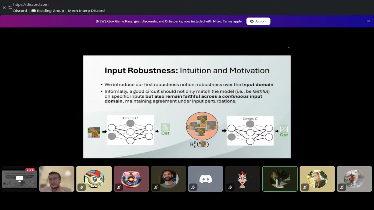
- [10:30](https://www.youtube.com/watch?v=ePbDEFuaraw&t=630s) Input Robustness certifies that a discovered circuit remains faithful across an entire continuous perturbation domain around an input, verified via a dual-branch Siamese Network Encoding.
- [15:51](https://www.youtube.com/watch?v=ePbDEFuaraw&t=951s) Patching Robustness ensures a circuit maintains faithfulness under all dynamically feasible activation values that non-circuit components could attain across an input neighborhood.
- [21:29](https://www.youtube.com/watch?v=ePbDEFuaraw&t=1289s) Continuous input perturbation bounds fit vision models naturally, whereas applying formal verification to language models would require defining continuous domains over latent spaces or embeddings.
- [30:55](https://www.youtube.com/watch?v=ePbDEFuaraw&t=1855s) Using the α,β-CROWN verifier within a greedy iterative pruning loop achieves 100% certified circuit robustness on vision benchmarks (MNIST, CIFAR-10, GTSRB, TaxiNet) while maintaining competitive circuit sizes.
- [41:37](https://www.youtube.com/watch?v=ePbDEFuaraw&t=2497s) The authors introduce a theoretical hierarchy of circuit minimality: quasi-minimality, local minimality, subset minimality, and cardinal minimality.
- [44:14](https://www.youtube.com/watch?v=ePbDEFuaraw&t=2654s) Standard single-component greedy iterative search always converges to a locally minimal circuit, but can get stuck before reaching subset minimality.
- [49:30](https://www.youtube.com/watch?v=ePbDEFuaraw&t=2970s) Simultaneous input and patching robustness predicates possess the mathematical property of monotonicity, which guarantees that greedy iterative search reaches a subset minimal circuit.
- [53:35](https://www.youtube.com/watch?v=ePbDEFuaraw&t=3215s) The Minimum Hitting Set (MHS) algorithm leverages mathematical duality over circuit blocking sets to compute certified lower bounds and exact solutions for cardinal minimality.
- [56:01](https://www.youtube.com/watch?v=ePbDEFuaraw&t=3361s) While greedy search is computationally faster, the MHS blocking set search is embarrassingly parallelizable across multi-node clusters.
- [01:05:22](https://www.youtube.com/watch?v=ePbDEFuaraw&t=3922s) Tightening the deviation threshold δ or increasing the perturbation radius ε forces the discovered circuit to retain more components to maintain provable alignment.
- [01:12:37](https://www.youtube.com/watch?v=ePbDEFuaraw&t=4357s) Statistical verification offers a probabilistic relaxation (holding with probability 1 - γ) to trade deterministic certainty for increased scalability on massive networks.
- [01:15:43](https://www.youtube.com/watch?v=ePbDEFuaraw&t=4543s) Performing formal verification directly on continuous neural network representations avoids the loss of detail and manual effort inherent in decompiling models into symbolic code like Rust or RASP.
## Detailed walkthrough
### [00:00](https://www.youtube.com/watch?v=ePbDEFuaraw&t=0s) Introduction and Presentation Agenda
The session opens with Itamar Hadad welcoming attendees and introducing the paper *"Formal Mechanistic Interpretability: Automated Circuit Discovery with Provable Guarantees."* Itamar shares that this research formed the core of his Master's thesis and was recently presented at ICLR. While waiting for his co-author Shahaf Bassan to resolve technical difficulty joining the voice channel, Itamar lays out the talk's agenda. The presentation aims to bridge formal methods and mechanistic interpretability, moving from the foundational mechanics of circuit discovery to neural network verification, novel robustness definitions, empirical validation, and theoretical minimality bounds.
* **Paper Title:** Formal Mechanistic Interpretability: Automated Circuit Discovery with Provable Guarantees
* **Authors:** Itamar Hadad, Guy Katz, and Shahaf Bassan
* **Context:** Itamar's Master's thesis work, accepted and presented at ICLR.
* **Core Goal:** Transition circuit discovery from heuristic approaches to formal verification with provable guarantees.
[02:03](https://www.youtube.com/watch?v=ePbDEFuaraw&t=123s) Circuit Discovery Foundations and Formal Notation
Itamar frames circuit discovery as a central open problem in mechanistic interpretability. At its core, the goal is to isolate a sub-graph of a neural network—termed a "circuit"—that is uniquely responsible for a specific behavior or computation. The granularity of these computational graphs can range from individual neurons and layers to attention heads or convolutional filters. He highlights pioneer work in vision models by Chris Olah and others, as well as landmark language model investigations such as the Indirect Object Identification (IOI) circuit.
To establish mathematical rigour, Itamar formalizes the full neural network as a computational graph $G$. A candidate circuit corresponds to a sub-graph $C$, while the unselected components form the complementary set $C^c$. Evaluating a circuit requires "patching" the complementary components $C^c$ with fixed or baseline values $\alpha$. The full model's inference on an input $x$ is denoted $F_V(x)$, while the circuit's inference—operating with $C^c$ patched to $\alpha$—is written as $F_C(x; \alpha)$. Faithfulness is determined by a predicate checking whether the logit output of the patched circuit aligns with the full model within a bound $\delta$, using metrics like logit difference or absolute maximum difference.
* **Circuit Definition:** A sub-graph $C \subset G$ responsible for a target behavior or sub-computation within the full model.
* **Granularity Levels:** Neurons, layers, attention heads, or convolutional filters.
* **Patching Baseline ($\alpha$):** Common empirical choices include zero-patching or mean-patching non-circuit components $C^c$.
* **Faithfulness Predicate:** Evaluates whether logit alignment metrics between $F_V(x)$ and $F_C(x; \alpha)$ stay within a defined threshold $\delta$.
[06:30](https://www.youtube.com/watch?v=ePbDEFuaraw&t=390s) Motivation: Moving Beyond Heuristics in Circuit Discovery
Despite the rise of circuit analysis in AI safety research and theoretical complexity studies, existing discovery algorithms rely almost entirely on heuristics and local approximations. Itamar points out two major vulnerabilities in empirical approaches. First, standard faithfulness metrics only test discrete, finite sample sets; minor adversarial perturbations to an input can break circuit faithfulness entirely. Second, common patching choices like zero-patching or mean-patching are arbitrary heuristics without formal backing.
The main motivation of their work is to inject formal methods into this process, delivering guarantees that hold across continuous input spaces and patching ranges rather than single point evaluations.
* **Core Flaw in Standard Methods:** Reliance on discrete test samples leaves circuits vulnerable to small input perturbations.
* **Arbitrary Baselines:** Selecting fixed numerical patches (such as zero or dataset mean) introduces hidden assumptions into circuit evaluation.
* **Objective:** Replace heuristic estimations with formal, mathematically certified properties.
Before detailing their novel framework, Itamar provides a concise primer on neural network verification. A formal verifier takes a network $F_G$, an input specification defining a region of interest over inputs $X$ (such as an $\epsilon$-bounded perturbation ball around an image), and an output specification describing desired or unsafe model behaviors $Y$.
Verification formally proves whether the output specification holds for *all* valid inputs within the bounded domain. Even though neural network verification is inherently an NP-hard problem, modern specialized verifiers can efficiently solve complex instances to provide absolute mathematical guarantees.
* **Input Specification:** Bounded region around input $x$ (e.g., $L_\infty$ perturbation ball $\|x' - x\|_\infty \le \epsilon$).
* **Output Specification:** Boolean condition over outputs (e.g., preserving top-1 classification or constraining logit variance).
* **Computational Complexity:** NP-hard in general, but tractable for realistic sub-problems using state-of-the-art verifiers.
[10:30](https://www.youtube.com/watch?v=ePbDEFuaraw&t=630s) Input Robustness and the Siamese Verification Encoding
Itamar introduces the first formal property proposed in the paper: **Input Robustness**. Standard circuit evaluation checks if a circuit correctly replicates full model behavior (such as classifying an image as a "cat") on isolated test samples. Input robustness demands that the circuit remains faithful across an entire continuous perturbation domain around those samples.
An audience member asks whether the perturbation neighborhood is input-dependent or formally constrained. Shahaf Bassan joins the call at this moment, apologizing for the delay, and explains that while the verifier can handle arbitrary continuous domains, their paper evaluates $\epsilon$-neighborhoods surrounding specific target samples.
To certify input robustness algorithmically, the authors present a **Siamese Network Encoding**. This architecture duplicates the network into twin branches—the full model and the candidate circuit—fed by an input perturbation region. The verifier checks an output criterion asserting that the winning logit of the circuit stays aligned with the full model across every point in the continuous input space.
* **Input Robustness Definition:** Guarantees circuit faithfulness over a continuous input neighborhood rather than discrete point instances.
* **Siamese Architecture:** Constructs a dual-branch computational graph pairing the unconstrained full model with the patched circuit.
* **Formal Certificate:** The verifier returns a provable guarantee if output alignment holds across the entire perturbation volume.
[15:51](https://www.youtube.com/watch?v=ePbDEFuaraw&t=951s) Patching Robustness and Combined Verifier Encodings
The second major property introduced is **Patching Robustness**. Traditional circuit analysis evaluates circuits under fixed, arbitrary patch values $\alpha$ (such as zero or mean activation values). However, Itamar illustrates that perturbing $\alpha$ by even a small amount $\epsilon$ can degrade circuit accuracy and cause incorrect predictions.
Patching robustness solves this by requiring the circuit to remain faithful under *all feasible activation values* that complementary nodes $C^c$ could attain when the network processes any input within a continuous domain. To certify this, the authors design a specialized verification encoding: an upper network processes the continuous input domain to generate dynamic activation bounds, which are then transplanted directly into the complementary nodes of the lower circuit branch.
Itamar concludes this section by outlining an extended three-network verification encoding capable of certifying **simultaneous input and patching robustness**, ensuring that a circuit holds under input noise and activation variance at the same time.
* **Patching Vulnerability:** Fixed values like zero-patching can hide circuit failure modes triggered by slight activation shifts ($\alpha + \epsilon$).
* **Patching Robustness Definition:** Faithfulness certified against all dynamically feasible activations across an input domain.
* **Transplant Encoding:** Feeds real-time activation bounds from a full model branch into the complementary nodes of the target circuit.
* **Simultaneous Robustness:** Combines input and patching robustness into a unified three-network verification architecture.
<FollowUp label="Explore how the paper handles theoretical minimality bounds for discovered circuits." query="How does the paper formally define and prove circuit minimality using neural network verifiers?"/>
[21:29](https://www.youtube.com/watch?v=ePbDEFuaraw&t=1289s) Continuous Input Domains and Latent Space Perturbations
An audience member interrupts to ask a critical question regarding input robustness: whether the framework assumes a single continuous domain for a given output, and how it handles models with discontinuous input spaces or non-vision modalities. The speaker clarifies that this branch of their robustness definitions specifically targets vision models, where input spaces like image pixels naturally form continuous local neighborhoods. In contrast, discrete domains like language tokens cannot be perturbed continuously in a meaningful way at the token level, though one could evaluate continuous perturbations around token embeddings.
The discussion expands as participants explore how these formal notions might extend to other domains. A participant suggests that the most direct translation to language models would be verifying perturbations within a continuous latent space rather than over discrete token sequences. Another attendee suggests discrete perturbation domains, such as renaming variables in math or code execution tasks. The speakers agree that while existing works explore verification in latent spaces, applying their exact provable circuit discovery framework to discrete token inputs or variable-swapping transformations remains an open direction for future research.
- Clarified that while pixel values in vision tasks allow natural continuous $\epsilon$-ball neighborhoods, token-level language inputs are inherently discrete.
- Suggested extending formal verification to language models by defining continuous perturbation domains within latent spaces or embedding representations rather than raw tokens.
- Highlighted alternative domain-specific perturbation models, such as variable renaming in mathematical or code reasoning tasks.
- "Language. You can look at the continuous perturbations around embeddings, but this is something a bit different than continuous perturbations around tokens."
After addressing the domain question, the speaker transitions back to the core methodology, recapping how input robustness and patching robustness are verified using neural network verifiers. To systematically discover robust circuits, the authors build upon automated circuit discovery by introducing a greedy iterative framework. The algorithm traverses the neural network component by component—such as individual neurons in fully connected layers or entire convolutional filters in CNNs—and evaluates whether each component can be safely eliminated without violating the circuit's faithfulness requirements relative to the unpruned model.
The presenter contrasts two main algorithmic variants within this greedy discovery loop. The baseline approach relies on standard empirical sampling, measuring faithfulness over a fixed batch or sample set of inputs. In contrast, the proposed provably robust variant replaces empirical sampling with neural network verification queries, formally certifying that faithfulness holds across an entire continuous input or patching domain before pruning any component.
- Iterative traversal eliminates components one by one while continually evaluating output logits against the full model.
- Operates in a top-down or bottom-up order, retaining components whenever their removal causes faithfulness bounds to be violated.
- Baseline variant tests faithfulness empirically on discrete input batches, whereas the provably robust variant guarantees faithfulness over continuous input balls or activation ranges.
- "It basically traverses the network component by component... and tries to eliminate each one while preserving faithfulness."
[29:43](https://www.youtube.com/watch?v=ePbDEFuaraw&t=1783s) Experimental Setup and Benchmark Datasets
To evaluate the proposed framework, the researchers set up experiments across four distinct vision benchmarks, covering both image classification and regression tasks. The evaluation set consists of 100 input batches, generating a distinct certified circuit per batch. For image classification, they test on MNIST using a fully connected neural network (analyzed at neuron-level granularity), as well as CIFAR-10 and GTSRB (German Traffic Sign Recognition Benchmark) using convolutional neural networks (analyzed at filter-level granularity). For regression, they evaluate TaxiNet, a benchmark for autonomous taxi track navigation.
To perform the formal verification queries required by the provably robust algorithm, the authors integrate the $\alpha,\beta$-CROWN verifier. $\alpha,\beta$-CROWN is widely recognized as a state-of-the-art neural network verifier capable of computing efficient bound propagation and branch-and-bound verification for non-linear activations.
- Classification benchmarks: MNIST (fully connected network, neuron-level circuits), CIFAR-10 (CNN, filter-level circuits), and GTSRB (CNN, filter-level circuits).
- Regression benchmark: TaxiNet autonomous navigation model.
- Verifier choice: $\alpha,\beta$-CROWN verifier used to answer all neural network verification queries.
- Experimental scale: Evaluation conducted across 100 input batches to extract and certify individual circuits per batch.
[30:55](https://www.youtube.com/watch?v=ePbDEFuaraw&t=1855s) Empirical Results for Input Robustness and ResNet Case Study
The speaker presents the empirical results for input robustness, comparing the sampling-based baseline against the provably robust circuit discovery method under zero-patching within an $\epsilon$-neighborhood around input pixels. While the provably robust approach incurs higher computational runtime due to the expense of solving $\alpha,\beta$-CROWN verification queries, it achieves $100\%$ certified robustness across all benchmarks. Crucially, this complete robustness guarantee comes without a blowup in circuit size, yielding sub-networks of comparable size to those found by the baseline.
To illustrate what input robustness means in practice, the speaker presents a visual case study on a ResNet sub-circuit discovered on CIFAR-10. When a small amount of adversarial or imperceptible noise is added to an image of a bird, the circuit discovered by the baseline sampling method misclassifies the perturbed input as a "deer". In contrast, the provably robust circuit retains a few additional critical filters (highlighted in green), enabling it to maintain the correct prediction of "bird" under the same input perturbation.
- Results demonstrate a clear runtime-versus-guarantee trade-off: verification queries increase computation time but achieve $100\%$ certified input robustness.
- Discovered circuit sizes remain closely comparable between the baseline sampling method and the provably robust approach across all four benchmarks.
- CIFAR-10 ResNet example shows that baseline sampling circuits collapse under minimal noise (predicting "deer" instead of "bird"), whereas provably robust circuits retain crucial sub-structures to preserve accuracy.
- "Our method... although slower in times because of the use of neural network verification queries... achieve comparable circuit sizes while maintaining 100% robustness."
[34:20](https://www.youtube.com/watch?v=ePbDEFuaraw&t=2060s) Patching Robustness Evaluation and Sub-circuit Structural Overlap
The presentation turns to patching robustness, evaluating sub-circuits over feasible activation domains against standard baseline patching techniques, specifically zero-patching and mean-patching (setting hidden activations to the mean across a dataset sample). Similar to the input robustness findings, certifying patching robustness requires more execution time due to verifier overhead, but yields sub-networks with significantly higher certified robustness while maintaining small, comparable circuit sizes.
During the discussion, an audience member asks whether provably robust circuits are simply the unrobust baseline circuits with a few extra nodes added. The presenter clarifies that while robust circuits often overlap heavily with baseline circuits, they do not always simply add nodes. In several instances, the verified computation follows entirely different pathways through the network rather than just appending filters to the sampling-based solution. A co-author adds that the paper's appendix includes formal Intersection over Union (IoU) metrics analyzing the exact structural similarity and overlap across discovered circuits.
- Patching robustness tested against zero-patching and mean-patching baselines over continuous feasible activation ranges.
- Confirmed that provably robust circuits consistently achieve higher certified patching success rates with modest circuit sizes.
- Audience Q&A highlighted that robust circuits frequently share core components with baseline circuits, but can also reroute computation through alternative sub-graphs.
- Appendix includes quantitative Intersection over Union (IoU) measurements comparing node/filter overlap between baseline and certified circuits.
[37:46](https://www.youtube.com/watch?v=ePbDEFuaraw&t=2266s) Tuning Epsilon Bounds and Formal Verification vs. Empirical Sampling
A participant asks how one determines the appropriate perturbation radius ($\epsilon$) for training and interpreting circuits, noting that setting $\epsilon$ too large might introduce unrealistic noise. The speaker explains that the paper's appendix evaluates various $\epsilon$ values to show that the robustness margin between their certified method and empirical baselines remains consistent across different neighborhood sizes. Choosing the optimal $\epsilon$ in practice depends on the domain constraints and how broad a safety guarantee is required for the targeted use case.
The speaker highlights the core advantage of formal neural network verification: unlike empirical stress-testing, which can only sample a finite collection of noisy points or specific adversarial attacks, neural verifiers provide mathematical guarantees over all infinitely many possible perturbations within the continuous $\epsilon$-ball. Responding to another question about circuit uniqueness, the presenter notes that while altering $\epsilon$ or changing traversal directions yields different sub-networks, fixing the greedy ordering and noise bound guarantees deterministic circuit discovery.
- Sensitivity analysis across different $\epsilon$ radii in the appendix confirms that certified circuits consistently outperform empirical baselines regardless of neighborhood scale.
- Formal verification covers the entire continuous $\epsilon$-ball, guaranteeing safety against all possible intra-neighborhood attacks, unlike empirical sampling which misses unseen perturbation points.
- Deterministic behavior: fixing the greedy traversal order (e.g., end-to-start) and perturbation bound $\epsilon$ yields a single deterministic circuit output.
- "Using formal neural network verification we can check all the perturbations... neural verification allows us to achieve certification across all feasible perturbations in that epsilon neighborhood."
[41:37](https://www.youtube.com/watch?v=ePbDEFuaraw&t=2497s) Defining Formal Notions of Circuit Minimality
Having established the empirical results for input and patching robustness, the speaker transitions to the paper's second major theoretical contribution: formal guarantees for circuit minimality. In mechanistic interpretability, smaller sub-networks are preferred because reduced component counts directly enhance human interpretability. While the full neural network is trivially faithful to itself, formalizing what it means for a discovered circuit to be "minimal" requires rigorous mathematical definitions.
The presenter introduces four distinct hierarchical definitions of circuit minimality, ordered from weakest to strongest: quasi-minimality, local minimality, subset minimality, and cardinality minimality. To ground these theoretical definitions, the speaker introduces a running example featuring a Boolean network that processes inputs $x_1, x_2 \in \{0, 1\}$ through intermediate nodes $v_1$ through $v_6$, using XOR gates to aggregate signals toward the output.
- Smaller circuit size directly correlates with higher human interpretability, making minimal representations desirable.
- Establishes four formal notions of circuit minimality: quasi-minimal, locally minimal, subset minimal, and cardinality minimal (ordered from weakest to strongest).
- Introduced a Boolean network running example with inputs $x_1, x_2 \in \{0, 1\}$, internal nodes $v_1 \dots v_6$, and XOR aggregation logic to demonstrate theoretical minimality proofs.
- "Intuitively, smaller circuits in size are considered more interpretable... we want to have smaller circuits as possible. But what can be stated formally about the size of circuits?"
[43:15](https://www.youtube.com/watch?v=ePbDEFuaraw&t=2595s) Running Example: Boolean XOR Network and Exact Faithfulness
To ground the formal definitions of robustness and minimality, the speaker introduces a simplified Boolean running example. In this toy neural network, the overall model $G$ computes an output $Y$ from multiple inputs, which algebraically simplifies to returning just $X_2$. The speaker reminds the audience of the underlying Boolean algebra identities—specifically that "XOR of something with itself is zero, and XOR with zero is that something"—which causes the larger network graph to collapse into simply outputting $X_2$.
For this running example, the speaker defines the faithfulness predicate as strict exact equality across all possible inputs. Under this requirement, a candidate circuit is considered faithful if and only if its output matches the full network's predictions for every single input combination. Consequently, any valid discovered circuit in this setup must always evaluate to $X_2$ for all input states.
- Running example network $G$ simplifies algebraically via XOR properties: $X \oplus X = 0$ and $X \oplus 0 = X$.
- Faithfulness predicate is defined as exact input-output equality across all possible inputs.
- Target faithful behavior: Outputting $X_2$ for all input combinations.
[44:14](https://www.youtube.com/watch?v=ePbDEFuaraw&t=2654s) Defining Quasi-Minimal and Locally Minimal Circuits
Moving into formal guarantees, the speaker presents the hierarchy of minimality notions, beginning with the weakest definition: a **quasi-minimal circuit**. Given a network $G$ and a faithfulness predicate, a circuit is quasi-minimal if it contains at least "some element that removing it will break the faithfulness of the circuit." In the running example, considering the component set $\{V_1, V_2, V_3, V_4, V_5\}$, node $V_1$ acts as a critical anchor; taking $V_1$ out ruins the XOR chain, ensuring the remaining components fail to output $X_2$.
The speaker then introduces a stricter criterion: the **locally minimal circuit**. Rather than having just a single sensitive component, a circuit is locally minimal if "every element is a breaking point"—meaning the removal of *any* single individual component causes the remaining circuit to violate the faithfulness predicate. For instance, in the subset $\{V_1, V_2, V_3\}$, removing $V_1$ leaves $X_1 \oplus X_1 \neq X_2$, while removing $V_2$ or $V_3$ yields $X_1 \oplus X_2$, both of which fail exact equality with $X_2$.
Crucially, the speaker connects these theoretical definitions to practical discovery procedures. The team proves mathematically that a standard greedy iteration algorithm—one that sequentially eliminates components one by one as long as faithfulness is preserved—is guaranteed to converge to a locally minimal circuit.
- **Quasi-minimal circuit**: Contains at least one component whose individual removal destroys circuit faithfulness.
- **Locally minimal circuit**: Every individual component is a breaking point whose removal destroys faithfulness.
- **Theoretical guarantee**: Standard greedy iterative elimination always converges to a locally minimal circuit.
[47:14](https://www.youtube.com/watch?v=ePbDEFuaraw&t=2834s) Subset Minimality and the Limitations of Greedy Search
To address the shortcomings of local minimality, the speaker advances to **subset minimal circuits**. In a locally minimal circuit, taking away any *single* component breaks faithfulness, but a user might still be able to remove a *group* of components simultaneously and end up with a valid circuit. For example, in the locally minimal set $\{V_1, V_2, V_3\}$, taking out both $V_2$ and $V_3$ together eliminates the redundant $X_1 \oplus X_1$ terms and leaves a fully faithful circuit. Subset minimality eliminates this loophole by requiring that removing *any subset* of elements (single or multiple) renders the circuit unfaithful.
In the running example, the set $\{V_2, V_4\}$ forms a subset minimal circuit because $V_2 \oplus V_4$ computes $X_2$, and removing $V_2$, $V_4$, or both destroys the output logic. However, the speaker highlights a major theoretical limitation of current tools: the conventional greedy iterative discovery algorithm "is not guaranteed to reach a subset minimal circuit." The speaker notes that specific network configurations cause greedy elimination to get trapped in locally minimal states without reaching subset minimality.
- **Subset minimal circuit**: No proper subset of components can be removed without violating faithfulness.
- **Greedy search limitation**: Single-component greedy search fails to guarantee subset minimality and can get stuck in local minima.
- Example: $\{V_2, V_4\}$ requires all elements to compute $X_2$, leaving no removable sub-configurations.
[49:30](https://www.youtube.com/watch?v=ePbDEFuaraw&t=2970s) Monotonicity: Bridging Robustness and Subset Minimality
To overcome the limitations of greedy search and guarantee subset minimality, the speaker introduces the formal property of **circuit monotonicity**. Monotonicity dictates that if a subgraph is already a faithful circuit, "adding some neuron to existing circuit does not break its faithfulness." In other words, expanding a faithful circuit by incorporating additional neural network components can never cause it to become unfaithful.
The speaker reveals a critical theoretical connection discovered by the authors: simultaneous input and patching robustness predicates are naturally monotonic. Because robustness constraints force consistency over bounded input and activation neighborhoods, adding extra nodes preserves this stability.
This bridge leads directly to a key theoretical result: "under monotonicity... the iterative greedy algorithm converges to a subset minimal circuit." By combining greedy discovery with robustness-based faithfulness predicates, researchers can formally guarantee that the resulting circuit is subset minimal without having to run expensive multi-component elimination searches.
- **Monotonicity property**: Super-graphs of faithful circuits remain faithful upon adding nodes or components.
- Simultaneous input and patching robustness predicates are mathematically proven to be monotonic predicates.
- **Convergence theorem**: Under monotonicity, standard greedy iterative search is guaranteed to discover a subset minimal circuit.
[52:06](https://www.youtube.com/watch?v=ePbDEFuaraw&t=3126s) Cardinal Minimality, Circuit Blocking Sets, and Duality
The speaker turns to the ultimate benchmark in circuit discovery: **cardinally minimal circuits**. This represents the absolute strongest notion of minimality, defined as a faithful circuit such that "there exists no smaller circuit in size that is faithful." In the running XOR example, the smallest possible node subset capable of implementing the overall XOR behavior represents the unique cardinally minimal circuit.
To construct algorithms capable of reaching or bounding this absolute minimum, the authors flip the problem on its head using a mathematical duality framework. They define **circuit blocking sets**—sets of nodes or subgraphs whose complete exclusion from a candidate circuit is guaranteed to break faithfulness. Put differently, a blocking set represents a mandatory structural bottleneck; any valid, faithful circuit must contain at least one element from every blocking set.
- **Cardinally minimal circuit**: The smallest possible faithful circuit in terms of absolute component count / cardinality.
- **Circuit blocking set**: A set of components such that excluding all of them renders any remaining circuit unfaithful.
- Dual perspective: Shifts focus from finding minimal faithful subgraphs to identifying mandatory structural blocking sets.
[53:35](https://www.youtube.com/watch?v=ePbDEFuaraw&t=3215s) The Minimum Hitting Set (MHS) Algorithm and Lower Bounds
Building on the concept of blocking sets, the speaker introduces a duality theorem centered on the **Minimum Hitting Set (MHS)** problem. Reminding the audience of the classical computer science definition, a minimum hitting set is the smallest cardinality collection of elements that intersects every set in a given family. Under the assumption of monotonicity, the speaker establishes that "the minimum hitting sets of all circuit blocking sets... is actually a cardinality minimal circuit."
This theoretical duality motivates a practical discovery algorithm: rather than greedily pruning nodes from the full model, the algorithm systematically searches for blocking sets of increasing sizes—starting with singletons (individual critical neurons), moving to pairs, triplets, and beyond—and calculates their minimum hitting set.
The speaker highlights a crucial guarantee of this approach: stopping the search at any intermediate blocking set size yields a provable "lower bound on the cardinality minimal circuit." If allowed to run to completion across all blocking set sizes, the MHS algorithm is guaranteed to converge exactly to the globally smallest cardinally minimal circuit.
- **Duality theorem**: Under monotonicity, the Minimum Hitting Set of all circuit blocking sets forms a cardinally minimal circuit.
- **MHS Algorithm**: Systematically enumerates blocking sets by increasing size (singletons, pairs, triplets) and solves the MHS problem.
- **Anytime lower bound**: Terminating MHS search at size $k$ gives a certified mathematical lower bound on the smallest possible faithful circuit size.
[56:01](https://www.youtube.com/watch?v=ePbDEFuaraw&t=3361s) Empirical Evaluation on MNIST and Practical Runtime Trade-offs
The speaker transitions to empirical experiments conducted on the MNIST benchmark to compare the proposed methods. The experimental results plot discovered circuit size against runtime across quasi-minimal, greedy iterative, and MHS duality algorithms. The data confirms the theoretical guarantees: the MHS algorithm consistently lower-bounds the circuit sizes found by all other methods, proving that "you cannot achieve a smaller size than that."
While the greedy iterative algorithm runs significantly faster and often approaches near-minimal sizes, MHS requires higher computational overhead to compute true lower bounds and exact cardinal minimality. However, the speaker highlights a key architectural advantage of MHS: unlike iterative greedy search—which must evaluate components sequentially step-by-step—blocking set discovery can be fully parallelized. The team demonstrated this in practice by parallelizing the MHS blocking set search across 14 parallel worker nodes.
Concluding the presentation portion, the speaker summarizes the overall contributions: a formal framework for circuit discovery uniting input and patching robustness, verification-based certification, circuit monotonicity, and formal minimality guarantees ranging from local to cardinal minimality.
- Experiments conducted on vision models trained on the MNIST benchmark.
- MHS provides a tight lower bound on circuit size; greedy iterative search runs faster but lacks cardinal guarantees.
- Blocking set discovery is embarrassingly parallelizable and was executed across 14 parallel workers.
- Summary of contributions: Robustness predicates, formal minimality hierarchy, verification integration, and MHS duality.
[01:00:05](https://www.youtube.com/watch?v=ePbDEFuaraw&t=3605s) Q&A: Applying Formal Verification to Alignment and LLM Latents
Following the presentation, an audience member praises the clarity of the walkthrough, remarking, "I don't think I looked too much into like formal verification before, so this is pretty cool." The participant then pivots to AI alignment, asking whether this formal framework could be applied to ensure "internal circuits that don't include deception" or provide provable safety guarantees.
The speaker acknowledges that alignment is a "very interesting and important point," clarifying that while their current benchmarks focused on vision models and input perturbations, robustness against adversarial inputs directly relates to safety. However, when addressing language models and complex alignment properties like deception, extending these bounds remains an open research frontier. A co-author/speaker adds that future work involves expanding to other perturbation domains, such as "statistical variants" and searching within the "latent space domain" where semantic representations live in LLMs.
Another audience member suggests leveraging verifiable task domains to construct perturbations, proposing that "every time there is some verifiable output, you could generate synthetic data which should equal the same verifiable output," pointing to mathematical reasoning tasks as a prime domain for defining input neighborhoods.
- Q&A opens with praise for bringing formal verification into mechanistic interpretability.
- Alignment application: Vision benchmarks address input safety, but LLM deception/alignment requires defining perturbation domains in latent space.
- Future research directions: Latent space certification, statistical variants, and domain-specific semantic perturbations.
- Participant suggestion: Use synthetic data generation in verifiable domains (e.g., formal math) to define rigorous input neighborhoods.
[01:04:07](https://www.youtube.com/watch?v=ePbDEFuaraw&t=3847s) Q&A: Decoupling Epsilon and Delta Parameters in Robustness Guarantees
In the final Q&A exchange, a participant asks about the mathematical relationship between the parameter bounds used in the robustness definitions, specifically asking whether $\epsilon$ (the input neighborhood size) and $\delta$ (the output logit tolerance) are independent or if "epsilon depends on delta" as a functional condition.
The speaker clarifies that $\epsilon$ and $\delta$ are treated as independent hyper-parameters in their framework. Epsilon dictates the radius of the input perturbation ball $B_\epsilon(x)$, whereas delta defines the maximum allowed divergence between the full network's logits and the circuit's logits. While tightening $\delta$ forces closer logit alignment, the two parameters remain decoupled variables in the formal verification formulation, allowing flexible configuration depending on the strictness of the desired faithfulness metric.
- Parameter decoupling: $\epsilon$ controls input perturbation neighborhood radius; $\delta$ controls output logit divergence tolerance.
- $\epsilon$ and $\delta$ operate as independent variables rather than functionally dependent parameters in the verification setup.
- Flexible framing allows customizing verification bounds based on domain requirements and model sensitivity.
[01:05:22](https://www.youtube.com/watch?v=ePbDEFuaraw&t=3922s) Tuning Perturbation Bounds ($\epsilon$) vs. Circuit Faithfulness ($\delta$)
The discussion begins with a deep dive into the mathematical relationship between the input perturbation radius ($\epsilon$) and the model output deviation threshold ($\delta$). The presenters unpack the intuitive trade-offs: if one selects a larger $\epsilon$-ball (testing over a broader continuous neighborhood of inputs) alongside a tighter, smaller $\delta$ (demanding extremely high output alignment between the pruned circuit and the full model), the automated search algorithm is forced to include significantly more components. A stricter fidelity target over a wider domain naturally causes the discovered circuit to expand until it closely resembles the entire original architecture.
When asked whether the formal guarantees hold over *all* possible model inputs or just a specific evaluation batch, the presenters clarify their methodology. While one could theoretically attempt to certify the circuit across the entire valid input space—such as the full $[0, 1]$ pixel range for normalized images—such an unconstrained requirement is practically far too strong and leads to intractability or overly bloated circuits. Instead, the framework evaluates continuous $\epsilon$-neighborhoods centered around a chosen batch of representative sample inputs (e.g., a batch of image samples representing a class like "cars").
- The balance between $\epsilon$ and $\delta$ functions independently; varying one does not strictly dictate the other, though both shape final circuit size.
- The parameter $\delta$ directly parallels the threshold parameter $\tau$ used in classical circuit discovery algorithms like ACDC (Automated Circuit Discovery with Actions), which thresholds metrics like KL divergence.
- Lowering $\delta$ (or $\tau$) enforces higher faithfulness at the cost of larger, less minimal circuits, offering a controllable dial for interpretability granularity.
- Exploring alternative perturbation domains—such as continuous manifolds inside the model's latent representation space or semantically meaningful feature directions—is highlighted as a promising frontier for future formal verification research.
"If we take a bigger $\epsilon$ and a smaller $\delta$, the circuit will have to intuitively include more components to be aligned... smaller $\delta$ requires bigger alignment with the model, and bigger $\epsilon$ is over a bigger neighborhood."
---
[01:09:15](https://www.youtube.com/watch?v=ePbDEFuaraw&t=4155s) Latent Manifolds, Steering Vectors, and Feature Activation Spaces
The conversation shifts to connecting formal verification with recent empirical breakthroughs in representation reading and steering. Participants discuss whether formal perturbation bounds could be applied directly to internal activation spaces rather than raw input pixels. In particular, they reference recent research on finding continuous manifolds in activation space—such as work from Goodfire AI—which demonstrates that certain features lie along smooth, non-linear manifolds rather than simple linear directions.
The group brainstorms how formal verification techniques like $\alpha$-$\beta$-CROWN could be leveraged to certify circuit behavior under steering vectors or safety feature directions. A participant notes that steering along an identified manifold often preserves model capabilities far better than simple linear probes. By defining the verification domain along these non-linear feature pathways, one could formally test whether a circuit remains robust to smooth internal state shifts without breaking the underlying computational graph.
- Potential latent perturbation targets include steering vector neighborhoods, sparse autoencoder (SAE) feature directions, and biological prefrontal cortex-inspired sub-circuits.
- Formal verification could formally test the hypothesis that circuits are resilient to perturbations *along* a feature manifold while fragile to orthogonal linear perturbations.
- The presenters emphasize that while input-space verification is a necessary first step, generalizing neural network verification to internal latent states is fully compatible with their theoretical framework.
"You could find that circuits are robust to perturbations along the manifold but not in the linear direction, because moving linearly breaks how the model represents information—it doesn't move smoothly through the path where the circuit works."
---
[01:12:37](https://www.youtube.com/watch?v=ePbDEFuaraw&t=4357s) Soundness Guarantees: Deterministic vs. Statistical Verification
A participant raises a fundamental doubt about deterministic guarantees in complex neural networks: given the non-linear fuzziness of deep models, can any formal method truly offer a 100% ironclad guarantee that an unintended behavior will never occur? The presenters acknowledge the practical limits of exact deterministic verification and introduce the concept of *statistical verification* as a scalable alternative.
Statistical neural network verification relaxes the absolute 100% deterministic requirement in exchange for probabilistic guarantees (e.g., certifying that a property holds with probability $1 - \gamma$ above a chosen confidence threshold). This relaxation allows verification tools to scale to significantly larger, more complex network architectures that choke exact SMT or MILP solvers. The authors highlight that follow-up work—such as papers on "certified circuits"—has already begun expanding their deterministic foundation into these statistical regimes.
- Deterministic verification provides complete mathematical proof over the defined $\epsilon$-ball, but suffers from steep computational complexity barriers as network size increases.
- Statistical verification trades off absolute certainty to gain massive improvements in scalability and model size capacity.
- Reference is made to broader automated safety verification efforts by Max Tegmark's group and collaborators working on provable AI safety bounds.
"Statistical verification is a classic extension of what we did... the guarantee would be less strong, but it's more scalable and you have the flexibility where it doesn't need to hold 100% of the time, but for a probability above some threshold."
---
[01:15:43](https://www.youtube.com/watch?v=ePbDEFuaraw&t=4543s) Decompiling Transformers to RASP/Rust vs. Direct Network Verification
The group discusses alternative formal interpretability approaches, contrasting direct neural network verification with decompiling model weights into discrete source code (such as RASP or Rust). Returning to a paper previously read by the reading group—which decompiled small transformer models into explicit Rust programs—the participants evaluate whether translating neural networks into symbolic code makes formal verification easier or harder.
While verifying properties on a compiled Rust program allows standard software verification tools to be applied, the decompilation process itself suffers from severe limitations. Current decompilation techniques rely heavily on manually engineered pattern-matching templates and struggle to handle realistic, large-scale architectures without sacrificing model faithfulness. The presenters argue that performing formal verification directly on the continuous neural representation is often superior to verifying an approximate, human-unreadable decompiled program.
- Decompiling a transformer into symbolic code like Rust or RASP can yield tiny, highly interpretable code blocks for toy tasks, but fails to automate for complex architectures.
- Heavy manual effort is currently required to identify model patterns before decompilation can occur, limiting its end-to-end automation.
- Decompiling to a compressed program risks discarding subtle representation details, whereas direct neural network verification preserves exact model behavior within the tested region.
"I'm not sure that writing it as a giant Rust program that nobody understands is better than just doing formal verification directly on the network like you are doing here."
---
[01:19:03](https://www.youtube.com/watch?v=ePbDEFuaraw&t=4743s) Practical Solvers and Architecture Support ($\alpha$-$\beta$-CROWN)
In the closing technical exchange, a participant asks whether $\epsilon$-to-$\delta$ ball verification is theoretically possible for any arbitrary Multi-Layer Perceptron (MLP) or neural architecture. The presenters confirm that formal verification is exact and sound for networks using piecewise linear activation functions (such as ReLU), where the network can be unrolled into a set of linear constraints suitable for bound propagation and branch-and-bound algorithms.
For non-piecewise linear activations (like GelU, SiLU, or Softmax), modern verification engines utilize conservative convex relaxations and upper/lower bound approximations. The speakers point to state-of-the-art verifiers like **$\alpha$-$\beta$-CROWN**, which extend formal bound propagation to Vision Transformers (ViTs) and deeper neural architectures. However, they emphasize that verification engines currently operate with the highest performance and tightest bounds on Convolutional Neural Networks (CNNs), ResNets, and pure MLPs.
- **Piecewise Linear Activations:** Activations like ReLU permit complete, sound, and exact verification unrolling.
- **Non-Linear Extensions:** Smooth activations use bounding approximations, which are sound but may return "unknown" if bounds loosen excessively.
- **Tooling:** Verifiers like $\alpha$-$\beta$-CROWN allow formal bounds to be computed efficiently on GPUs for modern vision and MLP models.
- **Best Performance:** Formal verification scalability remains strongest on CNNs, ResNets, and standard feedforward MLPs.
"Under piecewise linear activations like ReLU, yes... in practice, tools like $\alpha$-$\beta$-CROWN are implemented for Vision Transformers, but scalability-wise it works best on CNNs, ResNets, and MLPs."
## Notable quotes
> [21:29](https://www.youtube.com/watch?v=ePbDEFuaraw&t=1289s) Language. You can look at the continuous perturbations around embeddings, but this is something a bit different than continuous perturbations around tokens. — Itamar Hadad
> [27:06](https://www.youtube.com/watch?v=ePbDEFuaraw&t=1626s) It basically traverses the network component by component... and tries to eliminate each one while preserving faithfulness. — Itamar Hadad
> [30:55](https://www.youtube.com/watch?v=ePbDEFuaraw&t=1855s) Our method... although slower in times because of the use of neural network verification queries... achieve comparable circuit sizes while maintaining 100% robustness. — Itamar Hadad
> [37:46](https://www.youtube.com/watch?v=ePbDEFuaraw&t=2266s) Using formal neural network verification we can check all the perturbations... neural verification allows us to achieve certification across all feasible perturbations in that epsilon neighborhood. — Itamar Hadad
> [41:37](https://www.youtube.com/watch?v=ePbDEFuaraw&t=2497s) Intuitively, smaller circuits in size are considered more interpretable... we want to have smaller circuits as possible. But what can be stated formally about the size of circuits? — Itamar Hadad
> [44:14](https://www.youtube.com/watch?v=ePbDEFuaraw&t=2654s) some element that removing it will break the faithfulness of the circuit — Itamar Hadad
> [44:14](https://www.youtube.com/watch?v=ePbDEFuaraw&t=2654s) every element is a breaking point — Itamar Hadad
> [47:14](https://www.youtube.com/watch?v=ePbDEFuaraw&t=2834s) is not guaranteed to reach a subset minimal circuit — Itamar Hadad
> [49:30](https://www.youtube.com/watch?v=ePbDEFuaraw&t=2970s) adding some neuron to existing circuit does not break its faithfulness — Itamar Hadad
> [49:30](https://www.youtube.com/watch?v=ePbDEFuaraw&t=2970s) under monotonicity... the iterative greedy algorithm converges to a subset minimal circuit — Itamar Hadad
> [52:06](https://www.youtube.com/watch?v=ePbDEFuaraw&t=3126s) there exists no smaller circuit in size that is faithful — Itamar Hadad
> [53:35](https://www.youtube.com/watch?v=ePbDEFuaraw&t=3215s) the minimum hitting sets of all circuit blocking sets... is actually a cardinality minimal circuit — Itamar Hadad
> [53:35](https://www.youtube.com/watch?v=ePbDEFuaraw&t=3215s) lower bound on the cardinality minimal circuit — Itamar Hadad
> [56:01](https://www.youtube.com/watch?v=ePbDEFuaraw&t=3361s) you cannot achieve a smaller size than that — Itamar Hadad
> [01:05:22](https://www.youtube.com/watch?v=ePbDEFuaraw&t=3922s) If we take a bigger ε and a smaller δ, the circuit will have to intuitively include more components to be aligned... smaller δ requires bigger alignment with the model, and bigger ε is over a bigger neighborhood. — Itamar Hadad
> [01:09:15](https://www.youtube.com/watch?v=ePbDEFuaraw&t=4155s) You could find that circuits are robust to perturbations along the manifold but not in the linear direction, because moving linearly breaks how the model represents information—it doesn't move smoothly through the path where the circuit works. — Audience Member
> [01:12:23](https://www.youtube.com/watch?v=ePbDEFuaraw&t=4343s) Statistical verification is a classic extension of what we did... the guarantee would be less strong, but it's more scalable and you have the flexibility where it doesn't need to hold 100% of the time, but for a probability above some threshold. — Itamar Hadad
> [01:15:43](https://www.youtube.com/watch?v=ePbDEFuaraw&t=4543s) I'm not sure that writing it as a giant Rust program that nobody understands is better than just doing formal verification directly on the network like you are doing here. — Audience Member
> [01:19:03](https://www.youtube.com/watch?v=ePbDEFuaraw&t=4743s) Under piecewise linear activations like ReLU, yes... in practice, tools like α-β-CROWN are implemented for Vision Transformers, but scalability-wise it works best on CNNs, ResNets, and MLPs. — Itamar Hadad
Presenting their ICLR paper, Itamar Hadad and Shahaf Bassan argue that circuit discovery in mechanistic interpretability can transition from heuristic approximations to formal verification with provable guarantees. By integrating formal verifiers like α,β-CROWN, their framework certifies circuit faithfulness against continuous input perturbations and arbitrary activation shifts while providing formal minimality guarantees.
Failure Modes of Empirical Circuit Discovery (6:30)
Mechanistic interpretability aims to isolate a sub-graph (circuit) responsible for a target model computation, but conventional approaches rely on discrete sample evaluations and arbitrary patching baselines like zero- or mean-patching. Hadad explains that these heuristics leave sub-networks vulnerable: minimal adversarial input noise can break circuit faithfulness entirely, and shifting a fixed patch value α by a small ε can degrade circuit accuracy and cause incorrect predictions.
Certifying Input and Patching Robustness (10:30)
To replace heuristic estimations, the authors introduce formal input and patching robustness properties. Input robustness guarantees that a circuit remains faithful across an entire continuous ε-perturbation neighborhood rather than on discrete points. To verify this, the authors develop a Siamese Network Encoding that pairs the full model with the candidate circuit to certifiably check that logit alignment holds within a threshold δ across the continuous domain.
Patching robustness extends this guarantee to internal representations, requiring the circuit to remain faithful under all feasible activation values that complementary nodes could attain when processing an input domain. The authors encode dynamic activation bounds from a full model branch into complementary nodes, and also formulate a unified three-network architecture to certify simultaneous input and patching robustness.
Empirical Performance on Vision Benchmarks (29:43)
The authors evaluated their greedy verification framework using the α,β-CROWN verifier across four vision benchmarks: MNIST (neuron-level), CIFAR-10, GTSRB (filter-level CNNs), and TaxiNet. Tested across 100 input batches, the provably robust method achieved 100% certified robustness against input perturbations and higher certified patching success rates than empirical baselines, while discovering sub-networks of comparable size.
A case study on CIFAR-10 ResNet showed that while a baseline sampling circuit misclassified a slightly perturbed bird image as a deer, the provably robust circuit preserved a few additional critical filters to maintain the correct prediction. Although robust circuits share core components with baseline counterparts, the authors noted they sometimes reroute computation along entirely different pathways rather than merely appending nodes.
Formal Minimality Hierarchy and MHS Duality (41:37)
Because smaller circuits are more interpretable, the paper establishes a formal hierarchy of minimality: quasi-minimality (at least one component breaks faithfulness if removed), local minimality (every single component is a breaking point), subset minimality (no subset of components can be removed), and cardinal minimality (the globally smallest faithful circuit). The authors prove that standard greedy elimination converges to a locally minimal circuit, but can get trapped short of subset minimality.
To bridge this gap, the authors demonstrate that simultaneous input and patching robustness predicates are monotonic (adding components preserves faithfulness), which guarantees that greedy iterative search achieves subset minimality. To address cardinal minimality, the authors formulate a duality framework using circuit blocking sets—bottlenecks whose complete exclusion destroys faithfulness. Computing the Minimum Hitting Set (MHS) over blocking sets yields anytime lower bounds and converges to cardinally minimal circuits, an approach the authors successfully parallelized across 14 workers on MNIST.
While the framework provides sound, deterministic guarantees on piecewise linear networks like ReLUs in vision tasks, the authors acknowledge that NP-hard verification overhead limits scalability. Extending provable circuit guarantees to discrete token inputs in language models, continuous latent manifolds, and complex alignment properties like internal deception remains an open research frontier, with statistical verification and latent-space bounds identified as promising directions.
[21:29] Itamar Hadad: Language. You can look at the continuous perturbations around embeddings, but this is something a bit different than continuous perturbations around tokens.
[27:06] Itamar Hadad: It basically traverses the network component by component... and tries to eliminate each one while preserving faithfulness.
[30:55] Itamar Hadad: Our method... although slower in times because of the use of neural network verification queries... achieve comparable circuit sizes while maintaining 100% robustness.
[37:46] Itamar Hadad: Using formal neural network verification we can check all the perturbations... neural verification allows us to achieve certification across all feasible perturbations in that epsilon neighborhood.
[41:37] Itamar Hadad: Intuitively, smaller circuits in size are considered more interpretable... we want to have smaller circuits as possible. But what can be stated formally about the size of circuits?
[44:14] Itamar Hadad: some element that removing it will break the faithfulness of the circuit
[44:14] Itamar Hadad: every element is a breaking point
[47:14] Itamar Hadad: is not guaranteed to reach a subset minimal circuit
[49:30] Itamar Hadad: adding some neuron to existing circuit does not break its faithfulness
[49:30] Itamar Hadad: under monotonicity... the iterative greedy algorithm converges to a subset minimal circuit
[52:06] Itamar Hadad: there exists no smaller circuit in size that is faithful
[53:35] Itamar Hadad: the minimum hitting sets of all circuit blocking sets... is actually a cardinality minimal circuit
[53:35] Itamar Hadad: lower bound on the cardinality minimal circuit
[56:01] Itamar Hadad: you cannot achieve a smaller size than that
[65:22] Itamar Hadad: If we take a bigger ε and a smaller δ, the circuit will have to intuitively include more components to be aligned... smaller δ requires bigger alignment with the model, and bigger ε is over a bigger neighborhood.
[69:15] Audience Member: You could find that circuits are robust to perturbations along the manifold but not in the linear direction, because moving linearly breaks how the model represents information—it doesn't move smoothly through the path where the circuit works.
[72:23] Itamar Hadad: Statistical verification is a classic extension of what we did... the guarantee would be less strong, but it's more scalable and you have the flexibility where it doesn't need to hold 100% of the time, but for a probability above some threshold.
[75:43] Audience Member: I'm not sure that writing it as a giant Rust program that nobody understands is better than just doing formal verification directly on the network like you are doing here.
[79:03] Itamar Hadad: Under piecewise linear activations like ReLU, yes... in practice, tools like α-β-CROWN are implemented for Vision Transformers, but scalability-wise it works best on CNNs, ResNets, and MLPs.
Original transcript
[0:00] So, this is sensitive. Do not wait for
[0:02] me.
[0:04] >> Okay. So,
[0:05] yeah, I'll uh
[0:07] I'll start and Shahaf hopefully will uh
[0:10] join us soon.
[0:12] Uh so, yeah, hello. Thank you guys for
[0:14] having us. I'm Itamar and uh
[0:18] I'll be presenting this work uh
[0:20] I did with Shahaf. It's actually my I'm
[0:23] I'm a soon-to-be PhD student and this is
[0:26] actually my master's uh thesis work.
[0:29] And uh we uh recently presented in uh
[0:33] ICLR uh
[0:35] uh so, one or two months ago.
[0:37] And yes, so hopefully Shahaf will be
[0:40] here and present himself, too. But uh
[0:43] maybe we can just start, so.
[0:48] Um I just want to Sorry for this just
[0:50] want to check if he's having Is there an
[0:53] option to join now or Okay, I'll just
[0:56] start, so.
[1:00] Okay, so just uh some brief like agenda
[1:04] what we will showing today. So, we'll be
[1:07] first showing
[1:09] uh the circuit discovery problem which
[1:10] our work uh
[1:12] is uh concentrated in and uh some
[1:15] motivation for a former perspective
[1:17] and we'll be
[1:19] Oh, here's uh Shahaf.
[1:22] I think he I think he joined. Okay.
[1:25] And we'll be doing some short
[1:27] preliminary about neural network
[1:29] verification.
[1:31] And then
[1:33] uh we'll be starting to show our uh work
[1:36] of of uh first introducing some
[1:38] robustness notions we
[1:41] defined and some empirical results uh
[1:44] where we achieved those and then uh some
[1:47] theoretical results concerning circuit
[1:49] minimality.
[1:50] So, yeah, let us just start. I think it
[1:51] will be more clear.
[1:53] And yeah, feel free to ask about
[1:56] everything and
[1:58] uh Shatov and I will be
[2:00] happy to discuss things here.
[2:03] So, just like
[2:06] short note about circuit discovery. So,
[2:08] circuit discovery is a an open problem
[2:11] in mechanistic interpretability, a
[2:13] central one.
[2:15] That concerns finding a circuit where
[2:17] circuit is a subgraph of a neural
[2:20] network that is responsible for some
[2:22] computation or behavior within the full
[2:24] network.
[2:26] And of course, like the examining
[2:28] granularity of this circuits,
[2:30] check varies. I mean, we can look at
[2:32] circuit of neurons or of circuit of
[2:35] layers or attention heads and that's uh
[2:38] something that can
[2:40] uh
[2:40] have a
[2:42] different granularity.
[2:44] And we know that some works that uh
[2:48] discovered circuits in vision
[2:51] like the one presented by uh
[2:54] uh
[2:55] and Chrisola and
[2:57] other works that concerns
[3:00] circuits so
[3:01] in
[3:03] language models like the one of the
[3:06] IOI circuit.
[3:07] And
[3:09] just to be more precise, we'll be giving
[3:12] some short methodology on like
[3:15] uh and definitions of circuits, mainly
[3:17] notation so we can have easier
[3:19] time talking about this.
[3:21] So, let's start with
[3:23] having some neural network whose
[3:25] computational graph
[3:27] is G
[3:28] and which again, the the granularity
[3:31] uh can vary. We can look at a graph or
[3:35] computational graph of neurons or or or
[3:37] of
[3:38] uh
[3:40] layers or attention heads or of uh
[3:43] filters of a convolutional network uh
[3:47] but uh
[3:48] once we have like this computational
[3:49] graph
[3:51] a circuit is induced
[3:53] by
[3:54] uh
[3:55] patching
[3:56] which means like setting the
[3:58] complementary of that circuit or that
[4:00] sub graph
[4:01] to some values. So, here we have this
[4:04] notation of C complementary which is the
[4:07] non-circuit
[4:09] um components.
[4:11] And we have also
[4:13] just
[4:14] uh I'll be quick with this notation. We
[4:16] denote
[4:17] as FV of X the inference of the full
[4:20] model G on X and
[4:22] FC on X
[4:24] with the complementary as alpha to
[4:28] inference through the
[4:30] um
[4:31] circuit with the patched in the comp-
[4:34] with the complementary of that circuit
[4:36] patched with some alpha.
[4:38] So, let's say
[4:39] um when we talk about zero patching, we
[4:41] have some sub graph C
[4:43] and we set everything that's not in that
[4:45] sub graph the complementary to zero and
[4:48] uh
[4:49] this is what uh
[4:50] this can be noted
[4:52] that way.
[4:53] So, just uh yeah,
[4:55] basically that's that's what we're
[4:57] talking about. We have the full model GM
[4:58] we have the circuit
[5:00] of the bold black lines here and
[5:03] the non-circuit components are patched
[5:06] with the alpha here in gray.
[5:08] And
[5:10] and how can we check if a circuit is
[5:13] faithful meaning it's indeed responsible
[5:15] for some behavior within the full
[5:17] network? Well, for that we use the
[5:19] faith- some faithfulness predicate which
[5:21] is just like
[5:23] um a predicate that's taking the logits
[5:27] of the circuit the the circuit with the
[5:30] complementary patched to some value and
[5:32] the logits of the full models
[5:34] and check their alignment under some
[5:38] metric. For instance, we can look at the
[5:39] logit difference which is common in this
[5:42] uh type of works checking that some
[5:45] logits are bounded by some delta between
[5:47] the full network and the circuit.
[5:51] And we can look at apps max and other
[5:53] types of
[5:55] metrics we we consider.
[5:58] And so the methodology is basically to
[6:00] have full model to run a forward pass
[6:03] getting some logits and then to have our
[6:05] circuit with the complementary patch to
[6:07] some value alpha which can be zero or
[6:09] mean patching or other choices.
[6:11] And check that the logits of the circuit
[6:14] and the logits of the full model are
[6:15] aligned according to some metric.
[6:18] And
[6:19] And if that's if that's the case then we
[6:21] can say this is a state for circuit that
[6:24] is indeed responsible to
[6:26] implementing the computation within the
[6:28] full network.
[6:30] And
[6:32] Obviously circuit analysis is a central
[6:35] problem also has been proposed for AI
[6:38] safety.
[6:39] And the recent work also studied this
[6:41] from a
[6:42] complexity theoretical lens. Uh
[6:45] formalizing many aspects.
[6:47] But
[6:49] despite this the existing discovery
[6:51] methods rely largely on heuristics or
[6:54] approximations.
[6:55] And
[6:57] for instance
[6:59] small perturbations in the input can
[7:04] achieve
[7:05] different results of circuit
[7:07] faithfulness.
[7:09] And also common patching choices putting
[7:12] like in the complementary what we
[7:14] denoted as alpha
[7:16] are
[7:17] also kind of heuristics.
[7:19] And we wish to give some formal
[7:21] perspective to
[7:23] to this process.
[7:26] And before starting by showing this
[7:29] formal perspective which concerns some
[7:31] robustness notions we present and
[7:34] and other elements we we first show
[7:37] a a short note about neural network
[7:39] verification which will be
[7:41] which we used in this work.
[7:45] By the way, Shahaf, are you here?
[7:49] Can you hear us?
[7:52] And okay.
[7:54] I think he's still not, so
[7:57] hopefully
[7:59] he'll be joining and be able to
[8:03] Okay, so
[8:05] the
[8:07] we'll be now just
[8:09] giving you whatever about the neural
[8:10] network verification, so
[8:12] uh
[8:13] neural network verification problem is
[8:15] that of having some network, which we
[8:18] again with that our notations FG.
[8:21] And and
[8:23] it takes some input X and outputs Y
[8:26] and we want to have some input
[8:28] specification over X, for instance have
[8:31] X uh
[8:33] uh if that's X is an image, we would
[8:35] like to have this image uh
[8:37] uh
[8:39] uh to to be
[8:41] bounded let's say by some epsilon, so we
[8:44] can have some noise up to
[8:46] an epsilon in every pixel.
[8:49] And we want to have an and we have
[8:51] another specification
[8:53] over the output, for instance
[8:56] that's the
[8:58] prediction of that network will still be
[9:00] cat or
[9:03] for instance.
[9:04] And
[9:05] neural network verification problem is
[9:07] about formally verifying that for all
[9:10] inputs that satisfy
[9:13] the input specification that for
[9:15] instance every all
[9:17] all values that that of pixels within
[9:19] some uh
[9:20] uh
[9:22] some range
[9:23] uh
[9:25] are
[9:26] uh uh
[9:27] uh for all inputs specification for all
[9:31] inputs that uh satisfy the specification
[9:34] we would like that the output
[9:36] specification to also hold or not hold
[9:39] if for instance if that's the output is
[9:41] we can you usually encode here some
[9:43] unsafe output specification for instance
[9:46] predicting that this cat image is a dog
[9:49] and then we can formally verify if under
[9:51] some perturbation domain over the input
[9:55] the network is always correctly
[9:57] predicting cat or not. And the there are
[10:02] neural network verifier that although
[10:04] this is an NP the NP-hard problem there
[10:07] are some
[10:09] um
[10:10] neural network
[10:12] verifiers that
[10:15] can
[10:17] solve this problem and uh
[10:19] basically allow allow us to
[10:23] uh
[10:24] to verify whether all
[10:26] inputs satisfy some property on the
[10:29] output.
[10:31] Okay, so now we just start by showing
[10:34] the
[10:35] robustness notions we the formal notions
[10:38] we present here.
[10:41] So
[10:42] uh we start by showing the first the
[10:45] first robustness notions the robustness
[10:46] notion
[10:47] which is the input robustness which
[10:52] this is actually really robustness over
[10:53] the input domain which basically means
[10:55] that
[10:57] um we would like our circuit not to be
[11:00] just correct on finite set of samples in
[11:04] this case correctly predicting that this
[11:07] sample of cat
[11:08] is indeed a cat
[11:10] but we would like it to be robust over
[11:13] this input input domain meaning we would
[11:15] like it to predict that
[11:18] also over a continuous perturbation
[11:20] domain
[11:21] around this cat
[11:24] sample
[11:25] it would be still correctly predicting
[11:27] cat. So each we we basically demand that
[11:30] our circuit will remain faithful which
[11:32] in this case means
[11:33] uh correctly predicting cat not only
[11:36] over a finite set of inputs, but over a
[11:38] continuous input domain.
[11:40] Um
[11:42] which makes sense because obviously a
[11:45] good circuit should match the full model
[11:47] and predict cat not over some specific
[11:50] example of
[11:52] cat, but also over a noised uh samples
[11:55] in the perturbation domains around them.
[11:58] Yeah. Any questions by now?
[12:01] So far, so good.
[12:03] Okay.
[12:04] >> I have one question. Um does this
[12:05] neighborhood depend on the input or no?
[12:09] >> Uh no. We can the it depends on the
[12:11] epsilon here, which yeah, we can look at
[12:14] the bigger perturbation domain or
[12:15] smaller. Uh if we take too big, then it
[12:18] will be very blurry. Uh let's say can
[12:21] get also very blurry uh
[12:23] uh samples, but yeah, it depends on
[12:26] >> Is it formally defined or you're doing
[12:29] the perturbation
[12:30] with the inputs themselves?
[12:32] >> It's Sorry again. Uh
[12:34] didn't hear.
[12:36] >> So, how exactly are you formally
[12:38] defining the kind of perturbation you're
[12:40] doing to the input?
[12:42] >> So, yeah, we'll be showing uh that this
[12:45] is something we can achieve by neural
[12:46] network verification. Uh we can
[12:49] have this input specification saying
[12:51] that we look on this
[12:53] perturbation domain
[12:55] and verify that indeed the circuit
[12:57] matches the full model and correctly
[12:59] predicts cat for all inputs in this
[13:00] perturbation domain.
[13:03] But for now, we just uh
[13:06] define this notion that we would like
[13:07] that
[13:08] uh not only some finite set of samples
[13:11] will be uh the circuit will be faithful
[13:13] on, but over a continuous input domain
[13:15] around them.
[13:16] to also be faithful on.
[13:20] >> I'll also update that I was able to join
[13:22] a few minutes ago, so sorry about uh
[13:24] being late.
[13:25] And to also address the question, uh
[13:28] basically, it could be also defined on
[13:29] any possible continuous domain like the
[13:32] the verifier could be used for any
[13:34] continuous domain, but
[13:36] in this paper we just take like a set of
[13:39] inputs and then look at surrounding
[13:43] around these specific inputs. Um
[13:47] Yeah, that's about to make sense.
[13:55] >> Okay, great. So, once we have this
[13:57] robustness notion, the question is how
[14:00] can we in practice say if one circuit is
[14:03] indeed input robust? How can we certify
[14:06] circuits that are input robust? Well,
[14:09] for that we use the neural network
[14:10] verification
[14:12] that we previously discussed. And
[14:15] and how can we achieve that with neural
[14:18] network neural network verification?
[14:21] Well, we introduce some Siamese encoding
[14:24] that basically duplicate the full model
[14:27] and the circuit.
[14:28] And uh uh
[14:31] what we do here is we take input
[14:34] neighborhood around the input. So, in
[14:36] that image of cat we previously
[14:39] saw, we can take a
[14:41] input neighborhood around that image of
[14:43] a cat.
[14:45] And we have the logits of the full model
[14:47] and the circuit. And we put here some
[14:49] criterion on the output, which means
[14:51] that the model and the circuit are
[14:53] aligned. For instance, they would can
[14:55] look that they are both the the win the
[14:58] winner logit of
[15:00] uh
[15:00] of of the cat class in both
[15:03] models is bounded by some delta or any
[15:06] other criterion we we would like. And
[15:08] with this encoding, we just feed that to
[15:11] the neural network
[15:13] verifier, and we can
[15:15] get
[15:16] a formal guarantee saying if the model
[15:21] and the circuit are
[15:24] the circuit is is robust uh
[15:27] with respect to that input neighborhood,
[15:29] meaning it
[15:30] uh
[15:31] its predictions are aligned with the
[15:33] full model around that perturbation
[15:35] domain.
[15:37] And okay, so that's just this is a way
[15:39] we present how to certify if a circuit
[15:42] is input robust. This how we uh
[15:44] uh in if it's implements our definition
[15:47] of
[15:49] uh input robustness.
[15:52] Okay, and the second uh
[15:55] notion we present here is the the one of
[15:58] patching robustness. So, as we said, a
[16:00] circuit is induced by patching the
[16:02] complementary of that circuit, all the
[16:04] components of the neurons that are not
[16:06] in that circuit
[16:07] but are in the full model to some value.
[16:10] And this choice is also uh somewhat uh
[16:14] ambiguous.
[16:15] I mean
[16:16] um existing patching choices can be zero
[16:19] patching or mean patching or other uh
[16:23] methods.
[16:24] But the the the the value to put on the
[16:28] complementary is somewhat um
[16:31] a choice that is uh
[16:33] uh a heuristic and and not uh uh one
[16:36] backed by formal guarantees.
[16:39] And for instance, uh
[16:42] the the
[16:43] basically we have here
[16:45] we should also uh remember that this
[16:48] th- this with these notions of patching,
[16:52] we basically evaluate on a finite set of
[16:55] activations like zero or mean.
[16:57] And that's maybe an example for that is
[16:59] we can have this circuit that
[17:02] gets some value alpha on the
[17:04] complementary
[17:06] and the circuit uh
[17:08] uh predicts
[17:10] correctly cat, but if we perturbate this
[17:13] and take some uh alpha plus some
[17:16] epsilon, we can have a a false
[17:18] prediction,
[17:19] which means that this choice of patching
[17:23] values basically influence
[17:25] the the circuit. So,
[17:27] we basically want to give some more
[17:29] formal notion here of uh
[17:31] of patching.
[17:34] And our definition is this. We basically
[17:37] want to have the
[17:39] circuit
[17:42] correctly predicting cat like that,
[17:45] which basically means that implementing
[17:47] what the full model does, not over some
[17:50] specific choice
[17:52] of activations,
[17:54] but rather on
[17:56] all feasible
[17:57] patching values
[17:59] that can be attained over an
[18:01] continuous input domain. So, if we look
[18:04] at this continuous
[18:06] input domain and we think
[18:08] if we take all the feasible activations
[18:11] that can be attained over this
[18:12] continuous input domain, we would still
[18:15] we would demand that our circuit under
[18:16] all these feasible activations will be
[18:19] correctly predicting cat like the full
[18:21] model does.
[18:22] So, that's our formal notion of patching
[18:25] robustness.
[18:27] Uh Shahaf, would you like to add
[18:28] something?
[18:31] >> Uh no, sounds great.
[18:33] >> Okay.
[18:35] So, so
[18:38] then we have this notion and
[18:41] we
[18:42] also here
[18:44] ask ourselves how can we certify
[18:46] patching robustness? So,
[18:49] uh same thing, we design this
[18:53] another encoding to achieve such
[18:55] patching
[18:56] uh
[18:57] robustness certification using neural
[18:59] network verification. So, in here we
[19:01] also duplicate the full model and the
[19:04] circuit,
[19:05] but to get this effect of uh
[19:09] considering all the feasible activations
[19:12] under some input domain, we basically do
[19:14] some
[19:15] uh
[19:16] neighborhood on the inputs. We specify
[19:19] some neighborhood on the input of this
[19:21] model
[19:23] of the upper network, sorry, which
[19:24] basically which is only used to
[19:27] to get the activations transplanted here
[19:31] in this uh
[19:32] uh lower circuit network.
[19:35] And then we uh
[19:37] we we we as you can see in the lines
[19:40] here the dashed lines here um show that
[19:43] we take the
[19:44] the patching uh the activations from
[19:47] this
[19:48] uh
[19:48] upper network. And we have here the
[19:51] logits of the circuit
[19:53] which we then define an output criterion
[19:56] that they will will be aligned with the
[19:59] logits of the full model. So, maybe I'll
[20:03] uh just uh repeat to to be more clear.
[20:04] So, we have this uh circuit network here
[20:07] that takes
[20:08] it's uh the the complementary of this
[20:11] circuit takes its activations from the
[20:13] upper network
[20:14] which is operating on a
[20:17] uh continuous input domain.
[20:20] And we and with in our output criterion
[20:22] is that this circuit with the with the
[20:24] transplanted activations uh is aligned
[20:27] with the full model. In this way we we
[20:29] show that we achieve
[20:30] the patching robustness uh notion of
[20:34] having the circuit uh
[20:36] correctly predicting uh
[20:39] uh so or aligned with the full model
[20:40] under all feasible activations attained
[20:42] over this domain.
[20:46] And and we feed that to a neural network
[20:48] verifier and get uh
[20:50] get uh certified at the definition we
[20:53] showed.
[20:56] Okay, so uh another thing we show just
[20:59] briefly that we can one can also have
[21:01] this encoding which we show that
[21:03] uh uses three networks to achieve a
[21:06] simultaneous input and patching
[21:08] robustness, which means that
[21:10] uh this is a circuit where it's robust
[21:13] uh under input perturbations while
[21:16] simultaneously
[21:18] uh
[21:18] and and also robust under the all the
[21:21] patching values that are attained over
[21:23] some patching neighbor. That's also
[21:25] something that can be achieved which
[21:27] with another encoding maybe a bigger one
[21:29] with three networks that we show.
[21:32] Okay, and
[21:34] so far this we we introduced two
[21:37] robustness notions, input robustness and
[21:38] patching robustness, and we showed how
[21:40] we can certify this using neural network
[21:43] verification.
[21:45] And now we just show how our empirical
[21:48] results uh
[21:50] back this and how
[21:51] what what is the experimental setup uh
[21:54] we used.
[21:55] So by the way, there's a question in
[21:57] chat if you want to answer it before
[21:58] moving there.
[22:00] Sorry, yeah.
[22:02] >> Uh
[22:02] could get, for example, be multiple
[22:05] continuous input domains?
[22:08] >> One moment. I'll
[22:10] answer in chat. I'm sorry, I did not I
[22:11] did not see the uh the chat here.
[22:14] Oh, I wait.
[22:15] >> If you want to open the chat, it's uh
[22:17] >> Yes.
[22:19] I just the question was like
[22:21] it says like is it like could there be
[22:23] multiple continuous input domains for a
[22:25] specific that lead to the same output?
[22:28] Couldn't there? Isn't this making the
[22:29] assumption that one continuous
[22:31] like all the
[22:33] the space to like generate one output is
[22:35] all one continuous domain.
[22:37] >> You you ask us
[22:39] uh sorry about the patching robustness
[22:41] or
[22:43] >> Or like the input robustness.
[22:45] >> Yes.
[22:47] >> Like how do you know for certain that
[22:49] for example, cat I know for like the
[22:51] image models possibly like I buy that
[22:53] they're all like in that one
[22:55] continuous input domain, but like what
[22:57] about like for other types of models?
[22:59] Couldn't there be models that like
[23:01] uh don't have like one set of in like
[23:04] maybe it's discontinuous. So, like it
[23:06] has multiple set of input domains.
[23:08] Uh how do you detect every single set of
[23:10] input domains? Because like I don't
[23:12] think they're all continuous.
[23:14] >> And yes, so here we basically focus in
[23:17] this work
[23:19] on
[23:20] in this part of the the robustness
[23:22] notions on
[23:24] on the vision domain that has this kind
[23:26] of input uh
[23:28] uh continuous continuous input. We I'm
[23:32] I'm I'm I hope I get get your question
[23:35] right, but you ask
[23:37] like if you have set of inputs and how
[23:38] you can do achieve continuous continuity
[23:41] over them or like in general about
[23:43] >> Well, how do you verify that like I
[23:45] guess is it just a property the image
[23:46] models that like the set of the input
[23:49] domain is continuous for like outputting
[23:51] cat cup for example?
[23:53] Is it like an assumption of the
[23:54] like uh I just don't know if the concept
[23:58] of like
[24:00] uh
[24:02] the don't like the domain for like I
[24:04] guess like the image of like the bunch
[24:05] of cats like you showed on the slides
[24:07] that one like the BPE
[24:09] Mhm. Like that's the notion in image
[24:12] models.
[24:13] I guess
[24:15] >> Yes, in an image model obviously it's
[24:17] not just about one sample like you can
[24:20] take uh
[24:21] a a lot of samples and and and go and
[24:23] have some uh
[24:26] addition like of their
[24:28] of their surrounding neighbors.
[24:30] So, that I mean this is not we're not
[24:32] just talking about a single sample, but
[24:35] uh yes, it's maybe easier to think about
[24:39] and on vision domain than other domains
[24:41] that continuous continuous perturbations
[24:45] around the input are not uh
[24:47] uh very meaningful like for instance
[24:50] language. You can look at the continuous
[24:53] perturbations around embeddings, but
[24:54] this is something a bit different than
[24:57] continuous perturbations around tokens.
[25:00] I mean
[25:01] >> Yeah, I just don't think this would
[25:02] apply to tokens and I was like
[25:05] but that that's like that was my gut
[25:06] instinct for tokens. So I wasn't sure
[25:08] like I guess this is just proven for
[25:10] image models.
[25:12] >> Yes, it's
[25:13] image or if we look at the we also
[25:15] experimented with some uh
[25:18] Also in yeah, mainly for image or other
[25:21] types of data but yeah, for language and
[25:23] tokens it's a bit different set up than
[25:26] this part of the input.
[25:27] >> I guess that the classic extension I
[25:30] guess that the classic extension of this
[25:31] to language would be to produce some
[25:34] perturbation over a latent space not
[25:37] necessarily around the
[25:40] uh tokens or something like that cuz
[25:42] it's a latent space.
[25:44] Yeah, there are some works that do it
[25:46] generally verification in the latent
[25:48] space
[25:49] for language.
[25:51] I guess that that would be like the the
[25:53] most direct way to extend this.
[25:57] But this this is something that of
[25:58] course
[25:59] needs to be done in a future work.
[26:02] >> Okay, how about
[26:05] How about for math for example, changing
[26:08] names of variables for example?
[26:10] Uh
[26:11] That could be a perturbation maybe.
[26:14] Yeah, I guess I guess that there are
[26:15] lots of different perturbation domains
[26:18] that uh
[26:19] uh one can think about.
[26:23] Uh yeah, each one will provide a
[26:26] different guarantee
[26:27] of course. So
[26:30] I guess depending on the context you
[26:32] could think of different potential
[26:34] perturbation domains.
[26:38] >> Thanks.
[26:42] >> For some reason I don't see the chat
[26:44] here. Let's see. Um
[26:46] >> Um if if you go to the if you go to the
[26:49] stream and click on top right, there's a
[26:53] bubble
[26:54] kind of button
[26:55] that opens it.
[26:56] >> Ah, ah, yeah, yeah, yeah, yeah, great.
[26:57] Thank you. That was uh
[27:00] Got it.
[27:01] >> Okay.
[27:02] >> Yes, thanks.
[27:04] Um so,
[27:06] let's go back to Yes, so
[27:09] we showed as we said two notions of
[27:12] input robustness and patching
[27:13] robustness, and we showed that we can
[27:15] certify this
[27:17] once we have some circuit to save that
[27:19] input robust or patching robust using
[27:21] some encodings we did that are fed into
[27:26] neural network verifier.
[27:28] And now we show some some of our
[27:30] experimental setup and the results. So,
[27:34] uh let's first talk about some
[27:37] general um
[27:39] uh algorithm we used,
[27:41] which is building on the automated
[27:43] circuit discovery algorithm.
[27:45] Uh we present this greedy iterative
[27:48] framework for circuit discovery.
[27:50] Uh well, this algorithm as you can see
[27:53] here in this um
[27:55] uh demonstration, it's basically
[27:57] traverses the network component by
[27:59] component, in this case a neurons,
[28:02] and tries to eliminate each one while
[28:03] preserving faithfulness. You see here it
[28:06] always checks the logits against uh
[28:09] another
[28:10] the full model.
[28:12] And it eliminates components if
[28:16] faithfulness is preserved, otherwise
[28:18] it's uh
[28:19] it keeps them until it reaches some
[28:21] discovered circuits. So, this is
[28:22] basically a
[28:24] greedy algorithm that runs component in
[28:27] this case uh
[28:28] and to start
[28:30] one by one, tries to eliminate them
[28:32] checking faithfulness, and ends up with
[28:34] some um
[28:36] uh discovered circuit.
[28:38] And
[28:40] uh we basically our experiments focus on
[28:45] taking this
[28:46] somewhere experiments focus on taking
[28:48] this greedy algorithm and
[28:51] checking two variants the baseline
[28:53] sampling based variant which
[28:57] basically
[28:59] it's
[29:01] faithfulness is the measured on some
[29:03] batch or like the set of inputs
[29:07] and our probably robust variant of this
[29:10] algorithm which
[29:12] certifies
[29:14] uh
[29:15] the input robustness or patching
[29:17] robustness on some continuous domain so
[29:19] here we can see like the basic pseudo
[29:21] code where we have some iteration of all
[29:23] components and
[29:25] we have the two methods one is
[29:28] evaluating faithfulness directly on uh
[29:31] some set of inputs and ours which
[29:33] certifies that
[29:35] across some input or patching domain
[29:38] like we showed with the neural network
[29:40] verification.
[29:43] And so
[29:45] just one moment before we see the
[29:47] results and discuss them we just say
[29:50] that we here focus on vision benchmarks
[29:53] uh
[29:54] we use a three classification task
[29:57] MNIST CIFAR-10 and GTSRB
[30:01] which is a a traffic sign recognition
[30:04] benchmark and another regression task
[30:06] which goes
[30:08] for taxi mask.
[30:10] And for regarding the we examine 100
[30:14] batches of uh
[30:17] uh of inputs obtaining a circuit per a
[30:20] batch
[30:22] uh I'll mention that the MNIST model is
[30:25] fully connected
[30:26] and
[30:28] neural network the others are uh
[30:31] uh CNNs and the granularity here is the
[30:34] in the CNNs we operate we look at
[30:36] circuits of filters and in the fully
[30:38] connected one we look at circuits of
[30:40] neurons.
[30:42] And for the neural network verification,
[30:44] we mentioned this verifier
[30:46] that we use. So, we used alpha beta
[30:49] crown verifier,
[30:50] which is considered to be state of the
[30:52] art in that field.
[30:55] And let's maybe show our first results,
[30:58] which are the input robustness circuits
[31:00] results. So, as said, we compare our
[31:03] sampling-based baseline and our probably
[31:06] robust method.
[31:07] For the input robustness
[31:10] experiment, we use zero patching. We
[31:13] later have another
[31:15] experiment that we do on the patching
[31:17] robustness, but for this we use zero
[31:19] patching and we measure robustness over
[31:21] some
[31:22] input neighborhood
[31:24] epsilon around the
[31:27] around the pixels.
[31:29] And we report we report the average
[31:31] robustness as well as the average
[31:33] circuit size for the
[31:36] two methods and
[31:39] over the four benchmarks.
[31:41] So, here what we can see is that we have
[31:45] this uh
[31:46] sampling-based circuit discovery, which
[31:48] is the baseline, and ours our probably
[31:52] robust variant, and
[31:54] we can see that
[31:56] our method uh
[31:59] uh although slower
[32:01] in times because of the use of a neural
[32:04] network verification queries that are
[32:06] sometimes computationally expensive,
[32:09] uh so, it's it is uh
[32:12] somewhat more expensive in time
[32:14] comparing to the sampling-based
[32:16] the baseline uh
[32:18] the baseline times, but we showed that
[32:21] we achieve comparable circuit sizes this
[32:25] while maintaining 100% robustness, and
[32:29] which is the result of us being
[32:31] certifying that, comparing to lower
[32:33] rates on the baseline our
[32:36] So, we see here some trade-off in time,
[32:39] but
[32:40] uh
[32:41] we see that we can achieve comparable
[32:43] circuit sizes with
[32:46] uh 100% robustness comparing to much
[32:49] lower rates on the baselines.
[32:51] Um
[32:55] So, uh
[32:57] and maybe some illustrative uh
[33:01] uh
[33:03] uh figure of that can be this,
[33:05] where we can see in this case that's a a
[33:09] resonant circuit, which is
[33:12] a part of the circuits we found on the
[33:14] CIFAR-10 benchmark, where we have here
[33:17] the baseline on the upper part, and this
[33:21] is the circuit discovered by the
[33:23] baseline method of filters. You see them
[33:26] here in blue.
[33:27] And
[33:28] when this circuit
[33:30] gets some noise, the image of bird,
[33:33] although the noise here is barely seen,
[33:36] but it is some
[33:38] There is some noise here, apparently,
[33:39] and
[33:41] uh
[33:41] when it gets it this noise, the input of
[33:45] bird, it falsely classifies it as deer,
[33:50] whereas our probably robust method
[33:53] discovered circuits, while it retains
[33:55] some more filters, you can see the see
[33:58] them here in green,
[34:00] it correctly predicts it as bird. So,
[34:02] that's basically maybe an illustration
[34:04] of the
[34:05] input robustness notion that uh
[34:10] we certify and can achieve in our
[34:13] framework.
[34:16] And okay, and the second uh
[34:19] result we would like to show here is the
[34:20] is that of the patching robustness, and
[34:23] so, we also here examine patching
[34:26] robustness over some patching domain,
[34:28] which is uh
[34:30] the feasible activations attained to
[34:33] understand continuous uh
[34:35] uh indeed neighborhood.
[34:38] And we compare our method which
[34:41] certifies that against some baselines
[34:43] which are zero patching and mean
[34:45] patching which is uh six thing
[34:47] activations to some
[34:50] uh mean over selected uh sample set.
[34:54] And here we have uh the two baselines
[34:57] and our method and we can see that
[35:00] uh again uh we have the some trade-off
[35:03] in times but
[35:06] uh
[35:08] uh we we see here that again we can
[35:11] achieve comparable circuit sizes
[35:14] to the baselines
[35:15] uh while maintaining um
[35:18] higher uh rates of robustness.
[35:22] Um
[35:27] Yes.
[35:30] I see here some question in chat.
[35:32] Looking at the immediate results and
[35:36] Uh yes, so that's a great question um
[35:41] Uh so um
[35:43] mostly uh the
[35:45] uh if
[35:46] I was asked here if uh
[35:48] robust circuits mostly contain the same
[35:50] components at the unrobust plus a few
[35:52] nodes.
[35:53] So
[35:55] uh
[35:56] that is something that they yeah we
[35:58] we've encountered uh and also
[36:00] a few times. It's not always the case uh
[36:03] but
[36:04] usually I mean you can think of it as
[36:08] uh
[36:09] that
[36:10] sometimes I mean it's it
[36:12] it's not uh
[36:14] it it this is not the case that it it
[36:16] includes the just additional uh
[36:19] uh figures but
[36:21] uh
[36:21] it it largely it often intersects with
[36:25] the ones discovered by the
[36:27] something isn't variant and
[36:30] here uh yes it did it is the case that
[36:33] the
[36:34] some filters are added but it that's not
[36:36] always the case. So maybe it maybe I
[36:37] answered that uh
[36:40] uh
[36:41] my explanation was a bit uh
[36:43] unclear but
[36:44] we sometimes see that yeah this is just
[36:46] some added filters but sometimes not and
[36:49] it's not always the case that
[36:51] sometimes the computation is done
[36:52] through other routes uh
[36:55] and it's not only adding some
[36:57] more filters to the baseline one.
[37:01] >> We also have in the appendix analysis of
[37:05] the
[37:06] uh IOU in intersection over union and
[37:09] the measures like that that show
[37:13] relations between between these
[37:15] different circuits that were found in
[37:17] the experiments. So this analyzes this.
[37:27] >> Okay.
[37:30] Uh sorry. Yeah.
[37:34] Uh
[37:35] okay I see that someone is typing so I'm
[37:38] going to give you a little wait for
[37:39] another question.
[37:41] Um
[37:46] How do we know when to stop adding more
[37:48] noise as into the train to interpret
[37:49] into much noise so contact the pro uh
[37:52] Okay so regarding the noise so yeah
[37:55] that's a a great question how would do
[37:57] we choose what neighborhood to look on
[38:00] uh to examine and we do some uh
[38:04] variations of this in the appendix two
[38:06] we
[38:08] uh
[38:08] we can we we observe uh several uh
[38:13] uh
[38:13] different values for this epsilon which
[38:15] means several
[38:17] different sized uh
[38:19] uh neighborhoods
[38:21] and
[38:22] uh we showed her to that
[38:24] this distinction between the baseline
[38:26] and
[38:28] the robustness of our probably robust
[38:30] method and the baseline also
[38:32] it's
[38:34] is preserved the difference between
[38:36] these two.
[38:37] But yeah, that's a good question like
[38:39] what uh
[38:40] epsilon should you be should we pick? I
[38:43] guess
[38:44] uh
[38:45] uh it depends on the
[38:49] on the
[38:51] the
[38:52] the the level of
[38:53] uh
[38:55] uh
[38:56] the the the specific type of inputs and
[38:59] uh
[39:01] and
[39:02] what what the circuit we want to to have
[39:05] eventually
[39:07] and
[39:08] and
[39:10] I see also in some context we probably
[39:12] can't try
[39:14] and
[39:15] all possible perturbations to be one so
[39:17] then the second one
[39:18] and we can't make it one
[39:21] Uh
[39:22] so here
[39:24] that's the maybe the the thing we we
[39:27] show here that using formal neural
[39:29] network verification we can check
[39:31] all the perturbations. I mean it's it's
[39:34] not just uh
[39:36] uh
[39:36] uh
[39:37] we examine some set of perturbations and
[39:40] neural verifications allows us to
[39:42] uh
[39:43] achieve
[39:45] uh certification across all feasible
[39:47] perturbations in that epsilon
[39:50] neighborhood.
[39:52] Uh so
[39:53] >> Okay, I see.
[39:55] Yeah, my thought was also that
[39:57] for some tasks uh
[40:00] like you could design so so a lot of
[40:02] different perturbations that you just
[40:04] don't capture with the
[40:06] like when you are defining the
[40:07] neighborhood. Uh
[40:08] >> Yeah.
[40:09] >> So
[40:11] >> Yes, here we can
[40:13] >> some attacks
[40:14] that are not just adding noise for
[40:16] example.
[40:17] Uh
[40:19] >> Yes.
[40:20] So,
[40:21] that's but that's a good also thing that
[40:24] uh
[40:25] I also
[40:26] come to think about and could you find
[40:29] multiple circuits? Uh
[40:31] I mean uh so here we look at this greedy
[40:35] uh
[40:37] the traversal and in that case we yeah,
[40:40] we would go one by one and
[40:42] and we end up with some certain circuit,
[40:44] but uh obviously if we decide to go from
[40:48] start to end, then we can achieve a
[40:51] different circuit. And also the choice
[40:55] of epsilon here changes the circuit. So,
[40:58] we have some uh
[40:59] let's say design choices in this uh
[41:03] uh
[41:04] routine of circuit discovery that can
[41:06] and uh yield different circuits, but uh
[41:10] once uh we look at this end to start
[41:14] ordering and once we set this epsilon,
[41:16] we achieve the
[41:18] I mean
[41:19] the the because this is a greedy
[41:21] operation here, we achieve a
[41:24] greedy deterministic operation here, we
[41:26] we achieve the same circuit.
[41:27] Is that answering? Is that okay?
[41:31] >> Yeah, that's good. Thanks.
[41:33] >> Thank you.
[41:34] Uh okay.
[41:37] So, yeah, now we
[41:39] uh so we showed some two notions of
[41:41] input robustness, patching robustness.
[41:43] We show how can we achieve them and show
[41:46] our empirical results concerning them
[41:48] and now we
[41:49] we discuss second minimality, which is
[41:51] another formal guarantee we present
[41:53] here. And
[41:55] uh maybe this is the more
[41:57] this is the part where we show some more
[41:59] theoretical results.
[42:02] And so, intuitively uh smaller circuits
[42:07] in size are considered more
[42:09] interpretable. I mean, a full network is
[42:12] always a circuit. It It It's faithful to
[42:14] itself, but that's pretty trivial, and
[42:15] we want to have small
[42:17] smaller circuits as possible. And maybe
[42:21] but what can be
[42:24] stated formally about the size of
[42:26] circuits?
[42:29] And so, we first start by defining four
[42:35] definitions of circuit minimality.
[42:38] And from weakest to strongest as quasi
[42:41] locally subset cardinality minimal, we
[42:43] will be showing them
[42:44] briefly, and
[42:46] then we can prove a connection between
[42:48] these notions and circuit discovery
[42:50] algorithms. So,
[42:52] let's have this running example of a
[42:55] network of a Boolean network
[42:58] and that takes inputs X1 and X2 that are
[43:02] either zero or one.
[43:04] And it has some multiple nodes, which
[43:06] you can see here, V1, V2, V3, V4, V5,
[43:10] V6, and
[43:12] these are aggregated by XOR to
[43:15] output some Y. And this is a running
[43:18] example, which we will show our
[43:20] robustness
[43:21] minimality notions on.
[43:24] And so, uh
[43:26] if
[43:27] this big network actually simplifies to
[43:30] just computing uh
[43:32] return like outputting X2, if we can if
[43:34] you can do see the math here, just
[43:37] remember that XOR of something with
[43:38] itself is zero, and
[43:41] XOR with zero is uh
[43:44] the XOR of something with zero is that
[43:47] something, and
[43:49] basically, we will be looking with on
[43:52] uh in this running example on the case
[43:53] that where we demand our faithfulness
[43:55] predicates to be actual exact equality.
[43:57] So, basically, we want to find a circuit
[44:00] that is exactly
[44:02] outputting the same results for all
[44:04] inputs like the
[44:06] full network, which basically means that
[44:08] we will look for a circuit that's
[44:09] exactly that's always for every input
[44:12] output select two.
[44:14] And maybe I'll just show some uh
[44:16] the notions themselves and it will be
[44:18] more clear. So,
[44:20] our first weakest notion is
[44:22] quasi-minimal,
[44:24] which is
[44:26] uh
[44:27] given some network G like this and some
[44:30] faithfulness predicate, a circuit is
[44:32] quasi-minimal if it has some element
[44:35] that removing it
[44:37] will break the faithfulness of the
[44:39] circuit.
[44:40] So, we have some quite a quasi-minimal
[44:43] circuit is a
[44:44] a circuit of this full model that
[44:48] contains one element that if you take it
[44:50] out, then that circuit is no longer
[44:53] faithful. So, in this case,
[44:56] remember the full network is
[44:59] computing just X2, and we want to be
[45:02] having a circuit that is exactly like
[45:04] this full network, also predicting X2.
[45:06] So,
[45:07] in that case, if we look at
[45:10] um this set of components, V1, V2, V3, 4
[45:13] and 5,
[45:15] uh we have here some element that if we
[45:17] take that out,
[45:20] uh
[45:21] and this
[45:23] uh
[45:23] uh this group will this set will no
[45:26] longer be uh a valid circuit, which is
[45:29] the
[45:30] uh V1. If you take that out, the XOR of
[45:33] X1 of V2, V3, V4, V5 will not be
[45:37] resulting in
[45:39] X uh 2.
[45:41] So, that's an example of a quasi-minimal
[45:43] circuit.
[45:45] And
[45:46] a stronger notion, stronger definition,
[45:49] is the one of locally minimal circuit,
[45:51] which is a circuit that does not only
[45:53] contain one such element that taking it
[45:56] out will be
[45:57] breaking faithfulness, but
[45:59] all for any
[46:01] for
[46:01] for any of its element if
[46:04] every element is a breaking point. I
[46:06] mean, if we take every element and
[46:09] outside of the circuit will be breaking
[46:12] the circuit's faithfulness. So, in this
[46:13] case
[46:15] we can see that
[46:17] V1, V2, and V3 is is a locally minimal
[46:20] circuit because taking V1 taking V1
[46:23] obviously
[46:25] results in X1 XOR X1, which is not X2
[46:29] and taking
[46:32] V2 or V3 will be resulting with a
[46:34] different computation of X1 XOR X2.
[46:37] And this is not a
[46:39] So, yeah, this is also this is an
[46:40] example of a locally minimal circuit.
[46:44] And
[46:47] we show
[46:49] we prove that if we take some greedy
[46:51] iteration algorithm an exhaustive
[46:54] greedy iteration algorithm that always
[46:55] tries to eliminate in a greedy way the
[46:59] components while preserving
[47:01] faithfulness, this one
[47:02] converges to a locally minimal circuit.
[47:05] So, that's some connection we prove
[47:06] between
[47:08] this definition and
[47:10] discovery algorithms.
[47:13] And
[47:14] we will now show some stronger
[47:16] notions of minimality of circuits. So,
[47:18] we showed quasi and local. The The next
[47:21] one is subset minimal, which is
[47:24] a circuit that's
[47:27] not Locally minimal we said that every
[47:30] element is a breaking point. Here we say
[47:32] that a stronger notion of
[47:35] of that that's not just any element is a
[47:38] breaking point, but even taking a few
[47:42] elements at once
[47:44] will will will be a breaking point. So,
[47:49] uh
[47:51] uh maybe to make that more clear here in
[47:53] locally minimal we said that taking each
[47:55] element breaks faithfulness, but here we
[47:58] could have taken
[48:00] for instance V2 and V3 both and we will
[48:04] be resulting with a valid circuit.
[48:07] So, locally minimal means that we can
[48:09] you cannot take each one, but if you can
[48:11] take a subset out and still be
[48:14] uh
[48:15] uh
[48:16] obtaining a a valid circuit.
[48:20] So, subset minimal is as we said the
[48:23] stronger notion that not only that we
[48:26] have this circuit
[48:28] that taking any of its subsets
[48:31] uh
[48:33] uh
[48:35] outside of the circuit will will be
[48:38] breaking faithfulness. So, in this case
[48:39] V2 and V4 we we cannot uh
[48:43] uh V2 and V4
[48:44] if we take the XOR that's X2, but taking
[48:48] eliminating V2 or eliminating V4 uh
[48:51] breaks faithfulness. So, yeah, all all
[48:53] the subsets of this group is of this set
[48:55] is uh
[48:57] required.
[48:59] And
[49:01] we prove that the greedy iterative
[49:04] algorithm
[49:06] uh is not guaranteed to reach
[49:09] a subset minimal circuit.
[49:12] Um we show some uh
[49:15] examples of uh
[49:17] uh such uh
[49:20] uh circuits um
[49:23] which are some configurations that do do
[49:25] not reach subset minimal
[49:28] uh circuits.
[49:30] And the question is can we reach uh
[49:33] subset minimality, which is a stronger
[49:35] notion of minimality? How how can we
[49:37] achieve such strong
[49:39] minimality guarantee? And for that we
[49:41] introduce the notion of monotonicity,
[49:44] which is
[49:45] uh
[49:46] I mean, we use this notion of
[49:48] monotonicity to later prove that we can
[49:49] achieve subset minimality. And
[49:51] monotonicity is basically the notion of
[49:55] adding some
[49:57] neuron to
[49:59] existing circuit does not break its
[50:01] faithfulness. So, basically, if we have
[50:03] some circuit, which is a subgraph
[50:05] of the neural network, and we add some
[50:08] component to it. In In this case, this
[50:11] uh
[50:12] blue marked neuron,
[50:14] then that will be a faithful circuit,
[50:16] too. So, monotonicity says, basically,
[50:19] that if we have a faithful circuit, like
[50:20] this one here on the left, adding some
[50:22] component, in this case, the blue
[50:25] marked neuron,
[50:27] uh will
[50:28] will resulting in also a
[50:30] uh faithful circuit.
[50:33] And so, that's a property that uh
[50:36] we define.
[50:39] And interestingly, we show that some
[50:42] some connection between input and
[50:43] patching robustness and this property.
[50:45] We prove that a certain simultaneous and
[50:48] input and patching robustness setting,
[50:50] like we showed before, is actually a
[50:52] monotonic predicate. So, we we showed
[50:54] that
[50:56] uh interestingly.
[50:59] And what we prove is that under
[51:01] monotonicity, under this property we
[51:03] defined, the iterative greedy algorithm
[51:06] converges to a subset minimal circuit.
[51:11] Okay, so here we can we we we show
[51:14] theoretically that you can achieve these
[51:15] strong notions of minimality through the
[51:18] notion of monotonicity.
[51:22] Yeah, and and yes, and so, for this
[51:25] uh
[51:27] faithfulness predicate that is
[51:29] robustness based that we showed, then
[51:31] yeah, we can obtain subset minimal
[51:32] circuits.
[51:34] Okay, and just the the last uh notion of
[51:36] minimality we have is cardinally
[51:38] minimal, which is uh
[51:42] uh
[51:42] a circuit
[51:44] which is the strongest notion of
[51:45] minimality, which basically means that
[51:48] uh
[51:49] this is the circuit that the there there
[51:52] does exist no circuit with
[51:54] smaller cardinality
[51:56] that is a faithful circuit. So, a
[51:58] cardinality minimal circuit basically
[51:59] means a circuit that there exists no
[52:02] smaller circuit in size that is
[52:04] faithful.
[52:06] Uh in this case obviously here this is a
[52:09] cardinality minimal circuit because
[52:11] there is no smaller uh
[52:13] uh
[52:14] set than in cardinality than that that
[52:17] can
[52:18] implement the full network computation
[52:20] which is the external
[52:24] Okay, and can we say something about
[52:26] this strongest minimality? And so
[52:30] for that we do some
[52:32] we approach the problem from the
[52:33] opposite direction and we we present
[52:36] this duality, but first we just say what
[52:38] this duality is about. So,
[52:40] we introduce the notion of circuit
[52:42] blocking sets which are sets of uh
[52:45] subgraphs who
[52:47] uh that
[52:49] excluding them from
[52:51] any circuits breaks faithfulness. So,
[52:53] basically this is what can be seen as a
[52:54] neuron that
[52:56] uh
[52:57] uh
[52:58] excluding that from any circuits breaks
[53:00] the circuit's faithfulness. So, any
[53:02] faithful circuits should uh
[53:04] include them.
[53:06] And
[53:08] um in that case we here we we mark this
[53:11] in blue and you can see that
[53:13] any circuit that
[53:14] puts this in the complementary
[53:17] is resulting in a
[53:19] unfaithful uh circuit unfaithful uh uh
[53:23] predicate.
[53:24] And we establish a duality that uses
[53:27] this notion of circuit blocking sets to
[53:29] achieve cardinality minimal circuits
[53:32] uh through something called minimum
[53:33] hitting set. So, I I will be going real
[53:36] briefly on that, but just a minimum
[53:38] hitting set
[53:39] a reminder is
[53:41] uh
[53:42] if you have a few sets, then a minimum
[53:44] hitting set is a
[53:47] the the smallest cardinality uh
[53:50] of a set that intersects with each of
[53:52] these
[53:53] uh
[53:54] which with all of these sets.
[53:57] So, in this case, we have a few sets in
[53:59] different colors and green, orange, red.
[54:03] And the smallest uh
[54:06] set that intersects with all of these is
[54:09] two and six. So,
[54:10] you can see that.
[54:11] So, that's a minimum hitting set.
[54:14] And now we just uh
[54:16] let's talk about this duality. So, we
[54:18] show that under monotonicity
[54:22] the minimum hitting sets of all circuit
[54:24] blocking sets, all the
[54:27] uh components whose exclusion from
[54:29] circuits breaks faithfulness, so the
[54:32] minimum hitting sets of all these
[54:33] circuit blocking sets
[54:35] is actually a cardinality minimal
[54:36] circuit.
[54:38] Um
[54:39] so
[54:41] here we can
[54:42] uh we
[54:43] this way we we are able to uh
[54:46] to talk about the strongest cardinality
[54:49] one can obtain.
[54:51] And this leads us to this following
[54:52] algorithm of just searching blocking
[54:54] sets by increasing size. First, let's
[54:57] look for one neuron
[54:59] uh
[54:59] contrasting neuron and then take pairs
[55:02] of
[55:03] uh elements that break faithfulness and
[55:05] then triplets and computing their
[55:07] minimum hitting sets.
[55:10] And we prove that uh
[55:12] we can
[55:13] stop I mean we can look at all the
[55:18] all the uh
[55:21] uh enumerate all all the different uh
[55:24] sizes. I mean, we can go from singletons
[55:26] to pairs to triples and so on, but for
[55:28] any uh
[55:30] for any
[55:31] uh
[55:32] uh size we stop in
[55:34] we we we prove that they this algorithm
[55:37] uh returns a circuit whose size is
[55:39] actually
[55:41] a lower bound on the cardinality minimal
[55:43] circuit. And if we go all the way with
[55:47] and and enumerate all the possible uh
[55:50] uh sizes, then yeah, this algorithm
[55:52] converges exactly to the cardinality
[55:53] minimal circuit.
[55:55] And we showed that also empirically.
[55:59] And
[56:01] and
[56:02] here we can we experiment with that and
[56:04] we show that
[56:06] we have here some
[56:07] uh
[56:09] a quasi-minimal circuit, which is
[56:11] something that is not discussed here.
[56:13] And we also have uh
[56:14] the iterative
[56:16] algorithm circuits. We have here the
[56:18] circuit size.
[56:20] And the MHS uh size, the algorithm the
[56:23] MHS algorithm size, the duality
[56:26] algorithm size.
[56:27] And we show that first this MHS size
[56:32] always lower bounds other methods. I
[56:35] mean, you
[56:36] as we said, you this is the
[56:39] you you cannot achieve a
[56:41] uh
[56:41] smaller size than that.
[56:44] Uh although the iterative iterative
[56:46] search sometimes uh
[56:49] approaches near it, and we can see that
[56:51] uh
[56:52] uh
[56:53] some of
[56:55] uh the MHS sizes which were found to be
[56:58] faithful are also on this line.
[57:02] Uh I mean, MHS circuits, yeah. And uh
[57:05] here we can also see the trade-off in uh
[57:09] in
[57:10] uh time, where the
[57:13] uh
[57:14] the iterative search is uh
[57:19] is actually uh
[57:22] uses smaller circuits uh
[57:25] uh at the lower run time.
[57:28] And MHS is uh
[57:30] uh
[57:31] uh is slower, but it as we said uh
[57:34] approaches the cardinality minimal size.
[57:38] And uh for this experiments
[57:40] just save some note that was written
[57:42] here. And I forgot to say that we
[57:44] experiment over MNIST and
[57:46] this
[57:47] blocking sets that we check in each
[57:50] stage
[57:52] this can be done in parallel as this is
[57:53] not an iterative circuit discovery where
[57:57] we have to eliminate one component and
[57:59] then go for the another one. Here we can
[58:01] look for blocking sets
[58:03] in parallel and we did parallelize that
[58:06] over 14 workers. That's a technical note
[58:08] and
[58:09] uh yes, we can see here how the
[58:12] this NHS algorithm lower bounds the
[58:16] sizes of faithful circuits as
[58:19] uh
[58:20] as we showed
[58:21] uh
[58:22] with some trade-off in time.
[58:27] Um
[58:29] and
[58:30] so
[58:32] just uh
[58:33] a conclusion of what we showed is so we
[58:36] introduced this framework for circuit
[58:37] discovery
[58:39] we where we
[58:41] presented two notions of robustness
[58:43] input robustness and patching robustness
[58:45] and
[58:46] um some
[58:48] notions of formal guarantees uh
[58:51] concerning minimality of circuits.
[58:55] And we used neural network verification
[58:58] to
[59:00] uh obtain this certification of
[59:03] input and patching robustness
[59:05] and uh
[59:08] uh experimented with that against
[59:11] existing
[59:12] sampling-based baseline methods.
[59:16] And we showed also on our way to achieve
[59:18] stronger minimality the notion of
[59:20] circuit monotonicity and in the
[59:22] principal connections
[59:24] uh we we also showed between robustness
[59:26] and uh
[59:29] and uh
[59:30] monasticity and
[59:34] and then
[59:35] with that we
[59:38] we've been shown that the one can
[59:39] achieve the strongest minimality uh of
[59:42] circuit which is the cardinal we minimal
[59:44] circuits using some duality we we
[59:47] formed.
[59:49] Um
[59:50] so
[59:51] that's about it. We'll be happy to take
[59:54] questions if if there are.
[60:05] >> I just a comment. I uh thank you for
[60:07] explaining this. I don't think I looked
[60:09] too much into like formal verification
[60:10] before, so this is pretty cool.
[60:13] >> Yeah. No, thank you.
[60:15] Thank you.
[60:23] Thank you. But maybe a question.
[60:25] >> Yes. You talked about this in the
[60:27] context of uh
[60:30] of alignment essentially or
[60:34] or not much in this direction?
[60:37] >> In the context of alignment?
[60:40] >> Yes.
[60:43] So like
[60:45] >> Yeah.
[60:45] >> I don't know. Maybe like how to make
[60:48] probably guarantee
[60:50] to
[60:51] like uh
[60:53] internal circuits that don't include
[60:55] deception or something like this, for
[60:56] example.
[60:58] >> Yeah.
[60:59] Um yeah, well, that's a that's a very
[61:02] interesting uh an important uh
[61:05] a point and
[61:08] so here because we focused on the
[61:11] vision, we can think about uh
[61:14] uh faithfulness of
[61:16] uh
[61:17] for instance in the benchmarks we
[61:19] presented, we can have uh
[61:22] let's go back to that, sorry.
[61:24] And then
[61:26] here we would like to we
[61:30] in this kind of
[61:32] uh uh
[61:33] benchmarks of of or we can be
[61:36] uh talking about this uh
[61:39] safety of
[61:42] of the circuits. I mean, if we have a
[61:44] circuit using our
[61:47] our strong okay, we can achieve a
[61:48] circuit that is robust uh with respect
[61:51] to perturbations on the
[61:54] inputs here that are sometimes related
[61:55] to safety. But yeah, I guess your
[61:57] question mainly concerns or
[61:59] concerns uh
[62:01] language models that I have some more
[62:03] sophisticated notions of uh
[62:05] uh alignment. And we we we did not uh
[62:08] experiment with that, but yeah, that's a
[62:11] very
[62:12] important and interesting uh direction,
[62:14] for sure.
[62:22] >> I guess yes, I guess that that extending
[62:25] like
[62:27] that we're looking all the already for
[62:28] this for future work, but extending this
[62:30] to
[62:31] um other perturbation domains,
[62:35] uh statistical variants, and uh
[62:38] yeah,
[62:39] it's it's a it's a question of how to
[62:41] extend this to yeah, to to maybe to like
[62:44] like we spoke before about uh
[62:47] looking maybe at the latent space
[62:49] domain,
[62:50] everything
[62:51] how can we certify a domain that has
[62:55] some
[62:56] uh I guess meaningful semantic meaning
[63:00] in the context of language models. I
[63:02] think this is like uh
[63:04] an important question here.
[63:12] >> Yeah.
[63:12] >> Uh so so you can think maybe of this as
[63:14] like I guess a first step, and then
[63:18] uh using maybe a similar idea
[63:21] to extend this further.
[63:26] >> Or maybe every time there is some
[63:27] verifiable output, you could
[63:30] generate synthetic data which should
[63:33] equal the same verifiable output.
[63:37] In math, for example.
[63:39] So, some some of the math, not all of
[63:41] it.
[63:46] That could be one way to
[63:48] specify the neighborhood, maybe.
[63:51] >> Yeah, to talk about verification in this
[63:53] setup, yeah.
[63:56] Yeah.
[64:03] >> So,
[64:04] uh you Oh, go ahead.
[64:07] >> Yeah, so in in your definition for
[64:10] robustness, like uh these epsilons and
[64:13] deltas are like independent. And right,
[64:15] like epsilon does not have to depend on
[64:17] delta.
[64:18] >> Uh yeah, you
[64:20] You mean the the ones here, the epsilon
[64:22] and deltas?
[64:23] Sorry for being so slow on the
[64:25] scrolling, let's say.
[64:27] Yeah, you mean this
[64:29] these ones.
[64:33] Uh
[64:35] >> So, like
[64:37] like saying that
[64:39] uh epsilon depends on delta, would that
[64:41] be like a strong condition? Like for
[64:44] every delta, you can find an epsilon.
[64:47] >> Um
[64:48] so,
[64:50] I I don't think uh
[64:52] they are dependent dependent in that
[64:55] way. I mean, epsilon is is obviously the
[64:58] the neighborhood size, and delta is the
[65:00] the alignment, let's say, in logits. So,
[65:03] if you take a
[65:04] a smaller delta, then you force the full
[65:06] model and the circuit logits to be,
[65:08] let's say, closer. And it also depends
[65:10] on the faithfulness metric and and
[65:12] things like that, but
[65:14] and so
[65:16] I guess
[65:17] they are not directly dependent. You can
[65:20] have we actually included the variations
[65:22] in the appendix of both delta and
[65:24] epsilon.
[65:26] Um
[65:28] but I guess if we take uh
[65:31] a bigger uh
[65:33] epsilon and we take a smaller delta
[65:36] small delta and then it would be harder
[65:37] to I mean the circuit will
[65:40] have to maybe intuitively include more
[65:43] components to be aligned. I mean smaller
[65:46] delta maybe requires
[65:48] bigger alignment with the model and
[65:50] bigger bigger epsilon is over a
[65:54] a bigger neighborhood, so maybe that
[65:55] will require our circuits to be bigger
[65:57] and more like the full model.
[65:59] And I don't know if that answers, but
[66:01] yeah these are separate. I mean they can
[66:03] vary the epsilon delta and they are not
[66:07] that correlated or something.
[66:10] >> And also like in the definition
[66:13] like it's only it doesn't have to be
[66:16] true for all inputs, right? Like just
[66:19] you choose some batch of inputs.
[66:23] >> Uh you mean in our experiments the input
[66:26] robustness notion or
[66:28] >> The definition, yeah. Because you're not
[66:30] saying for all for all input X, you're
[66:33] just saying like
[66:35] for some batch of
[66:38] inputs X, right?
[66:39] >> Uh so
[66:41] we do talk about all inputs X like if
[66:43] like uh
[66:45] this the the main methodology is taking
[66:47] some batch of inputs. Let's say a batch
[66:50] of images of cars.
[66:52] So we consider uh continuous domains
[66:55] around each sample uh
[66:58] for instance that
[67:01] and that's how we
[67:03] we talk about it, so
[67:05] Uh yeah, we consider
[67:06] under I mean
[67:09] uh
[67:11] I mean the general methodology is taking
[67:14] some batch of inputs and finding
[67:18] I mean a sample set and finding a
[67:19] circuit.
[67:22] So we we we look at all the continuous
[67:26] input perturbations around all the
[67:28] samples.
[67:31] >> Like you you could theoretically look at
[67:33] the entire perturbation domain. Right?
[67:36] So so you could theoretically say okay
[67:38] if it's like an image and
[67:40] let's say it's normalized so it's
[67:41] between zero and one. So we're actually
[67:43] verifying that for the entire possible
[67:45] domain the circuit
[67:47] behaves like the original model. But
[67:51] this would probably be a too strong of a
[67:54] notion. So
[67:56] for this for this reason we're limiting
[67:59] the perturbation domain to be epsilon
[68:02] balls around a bunch of
[68:05] images that we know of. And
[68:07] as I said before like this uh
[68:10] looking at other different perturbation
[68:12] domains
[68:14] could be also interesting for future
[68:15] work like looking at the latent space or
[68:18] other looking for maybe perturbation
[68:21] domains that have some semantic meaning
[68:23] or other ideas could be interesting. And
[68:26] regarding the comment for on the delta
[68:29] I think this is like really similar to
[68:32] in the classic ACDC paper where they
[68:35] call tau. So they have this tau
[68:38] parameter that you're looking at the KL
[68:40] divergence
[68:42] metric will also will always be above
[68:45] some tau. And then you can play around
[68:47] with this tau. So if it's
[68:49] large
[68:51] right or small this this will there is
[68:54] some trade-off. So it's either that
[68:56] you'll have that the faith
[68:57] the circuit is I guess more faithful or
[69:00] that you'll have that the circuit is So
[69:02] if it's more faithful, it will be
[69:03] larger, and if it's
[69:05] uh less faithful, it will be smaller.
[69:07] So, it's a I guess some granularity
[69:09] level that uh you need to play with. Uh
[69:15] >> Or the perturbations on latent space, uh
[69:19] something that seems relevant is the
[69:21] recent uh good fire uh papers about
[69:25] finding finding manifolds on the uh on
[69:29] activation space.
[69:31] Uh
[69:32] where you know, they like claim some
[69:35] features are represented on some uh
[69:37] continuous manifold where as you can
[69:41] move on it and have the some part of the
[69:46] output or, you know, or something about
[69:47] some circuit change in a smooth way. It
[69:50] seems like
[69:52] there could be something there where you
[69:54] could
[69:55] do something like this to check that or
[69:58] something.
[70:01] >> Yeah, I think it's a interesting
[70:02] direction generally.
[70:05] Need to think about it a bit more, but
[70:07] but but yeah, I think any any extension
[70:09] to other perturbation meaningful
[70:11] perturbation domains uh could be really
[70:14] interesting direction.
[70:17] >> Yeah.
[70:18] Uh perturbations around steering vectors
[70:21] that are aligned in the directions,
[70:22] perturbations around the safe features
[70:25] that are also technical and damaged uh
[70:28] directions.
[70:29] Uh but this is something good more.
[70:31] And perturbations around the the
[70:33] manifolds as Victor said.
[70:36] Or the Or maybe also around circuits in
[70:38] the dorsolateral prefrontal from the
[70:41] biology of Alan's paper from a tropic
[70:43] for instance, that might work, maybe.
[70:45] Um somehow
[70:47] in latent space.
[70:49] >> Mhm.
[70:51] Uh yes yes, totally agree. I I I think I
[70:53] see this like as a first uh
[70:57] step like in formalizing some of the
[70:59] stuff in general and totally agree that
[71:01] there are lots of uh
[71:03] uh
[71:04] potential ways
[71:05] to define this.
[71:09] >> It is like
[71:10] >> No, go ahead.
[71:11] >> I think I guess like I was thinking that
[71:13] it seems like too cool like the the good
[71:16] fire people are you know were claiming
[71:20] things about
[71:22] uh
[71:23] you know how steering with the manifolds
[71:26] was was better than steering with the
[71:28] linear probes for example
[71:31] seems like they should be uh
[71:34] you should be
[71:36] formalized as some kind of something
[71:39] like this where say something about like
[71:43] you can you can easily more easily find
[71:45] circuits that only you're trying to find
[71:47] circuits you'll find that they are
[71:51] robust to perturbations through along
[71:54] the many fold but not on the linear
[71:58] direction because that breaks how the
[72:00] model represents because like that's in
[72:02] some sense
[72:03] moving from a path not you know moving
[72:06] as smoothly through the path where the
[72:08] circuit works.
[72:11] >> I need to think about it a bit more. I
[72:15] But yeah, I guess in in any place where
[72:18] you can have perturbations
[72:20] uh
[72:20] and you can use neural verifications to
[72:23] certify that in the end that's also
[72:25] applies to manifolds and
[72:28] I don't know.
[72:30] I would have some set of signal. Yeah, I
[72:32] don't I mean
[72:33] that's a very cool thing to think about.
[72:35] Yeah.
[72:37] >> I I I still have this feeling at least
[72:39] with these these neural
[72:43] models where the
[72:45] where is
[72:46] things are very fuzzy often that
[72:49] for sufficiently complex behaviors
[72:53] but like there's
[72:54] at least with everything I know so far
[72:56] there's not
[72:58] 100% guarantee that the model will not
[73:01] do something that you don't want for
[73:03] instance.
[73:04] instance
[73:05] I don't know even if you if you have
[73:07] some circuit and some perturbations
[73:08] around it and so on uh
[73:11] there might be some other
[73:13] equivalent circuit which you just didn't
[73:15] identify for instance.
[73:17] uh
[73:18] >> So there are extensions of neural
[73:20] network verification to uh
[73:23] uh there there are lots of works on a
[73:24] statistical verification as well. Um
[73:28] which is also like a classic I guess
[73:30] extension of a what we did. Um so there
[73:34] you could for example look at the some I
[73:36] guess statistical guarantee. It's not
[73:39] it's not necessarily 100% of the time
[73:41] but for some I guess uh
[73:43] probability
[73:45] uh statistic you want it to to hold.
[73:49] Um
[73:50] So I guess uh I don't know if that
[73:52] answers any of your question.
[73:54] Um
[73:56] So so the the guarantee would be like
[73:58] less strong
[73:59] um more scalable
[74:02] and you have this uh flexibility of it
[74:05] doesn't need to hold 100% but uh
[74:09] let's say uh
[74:10] uh would for
[74:13] for probability above some threshold
[74:15] let's say something like that.
[74:19] >> Yeah.
[74:20] Yeah I that's also good. Also maybe
[74:23] another question is are you familiar
[74:24] with what Max Tegmark and some others
[74:26] are doing in uh also trying to
[74:30] automatically verify or probably verify
[74:33] safeness uh
[74:35] of models basically.
[74:39] >> Which which which uh
[74:41] group are you talking
[74:42] >> I saw you sent that in chat. I see you
[74:43] sent that in chat. Yeah I I'm familiar
[74:47] >> And
[74:47] >> From from Max Tegmark Steve or or book
[74:50] >> boo boo also David odds
[74:52] and bunch of other people.
[74:54] Uh
[74:56] Yeah, these papers at the beginning. I
[74:58] haven't read those papers. So, I'm just
[75:00] if you if you're aware, I don't know.
[75:05] >> Yes, we look at them. And there there
[75:06] actually one paper that's
[75:09] that followed ours which is one
[75:12] extension that what I said for
[75:15] statistical guarantees.
[75:17] Uh
[75:17] that's called certified circuits.
[75:20] Uh
[75:22] You can also look at that one.
[75:24] Uh
[75:25] but I I don't know that specific paper
[75:26] you're referring to.
[75:28] Uh so, I'm going to definitely look it
[75:30] up as well.
[75:32] >> Yeah, thanks for the video. Looks good.
[75:35] >> Okay, thanks. Yeah.
[75:43] I
[75:45] I think
[75:46] I think those are also into like neuro
[75:48] symbolic systems where
[75:51] you have some more
[75:53] where you can do some formal stuff more.
[76:00] Yeah, maybe that's also thing.
[76:03] If you're generating only lean then
[76:05] or only rust then
[76:08] yeah.
[76:11] There you can have certain guarantees
[76:14] for every single input, I mean output.
[76:20] Oh.
[76:21] I'm not sure exactly what Mark Stegmark
[76:23] is doing though.
[76:25] Yeah.
[76:26] >> As there is also the paper
[76:28] for de-compiling transformers to rust. I
[76:31] don't know if
[76:33] >> Yeah, we read it on this reading group.
[76:35] >> Yes, yes. I saw it as well that you
[76:37] went over it. So, so in in rust you can
[76:40] also like uh
[76:42] verify certain properties.
[76:45] I guess uh yeah.
[76:47] Problem is like if you lose some of the
[76:49] faith faithfulness in the
[76:51] uh de-compiling process, I guess.
[76:54] >> Yeah, I don't think that
[76:56] that it's like a great way of
[76:59] de-compiling yet like the
[77:01] uh I don't remember that much of the
[77:03] paper. We'll have to go look at the
[77:04] paper, but I I I I I My big memory of it
[77:08] was not that
[77:09] uh great of a way of
[77:11] in practice for real models to to do the
[77:15] de-compile it, actually de-compile it
[77:16] the model.
[77:17] Uh Yeah, it it was mostly
[77:21] >> Yeah.
[77:23] >> Oh, sorry. It was mostly very simple
[77:24] circuits.
[77:25] >> Yeah.
[77:26] Uh
[77:31] I I think that it seems like it cut like
[77:33] some parts that were kind of
[77:35] not that automated. Like they they work
[77:38] because they
[77:40] they kind of did a lot of manual work of
[77:43] identifying some
[77:45] kinds of patterns in models and
[77:49] make it so they were detected when those
[77:52] happened, but it would be hard to
[77:55] do the same kind of thing they were
[77:56] doing for
[77:57] for everything. But yeah, maybe there is
[77:59] some nicer way of for you know,
[78:01] de-compiling things in RASP and and that
[78:05] that doesn't just give you like the
[78:07] model, but writing it as a giant RASP
[78:11] program that nobody understands.
[78:13] Uh
[78:15] Uh
[78:17] I mean I mean it's maybe if maybe if you
[78:19] nobody understands, you will still do
[78:21] formal verification it, but
[78:24] uh I'm not sure that that's better than
[78:26] just doing it like you are doing here
[78:28] with on the network directly. Uh
[78:34] >> Yes, I I I like the the main thing is
[78:36] like if you decompile to like a smaller
[78:39] model or to a smaller representation, it
[78:41] could be like a scalability-wise easier
[78:44] to deal with it, but the problem is that
[78:45] you you lose like
[78:47] probably a lot of like what the model
[78:49] represents in this decompiling process,
[78:52] but maybe there there's some trade-off
[78:54] here.
[78:56] That needs that can be explored, I
[78:58] guess.
[78:59] >> Yeah.
[79:03] So, like uh
[79:05] I don't know much about this formal
[79:07] verification, but like is it the case
[79:10] that with any MLP like you can verify if
[79:13] like a epsilon ball
[79:15] lands in a delta ball? Like is that
[79:18] possible for any
[79:20] neural network?
[79:21] >> Yes, but under piecewise linear
[79:24] activations, you can also have some
[79:26] approximations and
[79:28] non-piecewise linear, but let's say if
[79:30] your MLP uses piecewise activations like
[79:33] ReLU, then
[79:35] uh yes.
[79:37] >> Yeah, but there there's also extensions
[79:38] for like other activation functions. It
[79:41] is true that it uh
[79:43] it's like uh
[79:45] it's not complete, meaning that uh
[79:48] uh
[79:49] it doesn't have to converge uh to a
[79:52] final solution. It can also say like I
[79:54] don't know if it's not a piecewise
[79:56] linear, but in practice it
[79:58] there's also like a
[80:00] uh alpha-beta ground that is implemented
[80:02] on like a vision transformers.
[80:04] And then
[80:06] and stuff like that, but
[80:07] uh it works I think the worst the best
[80:10] on
[80:12] CNNs, ResNets,
[80:14] MLPs,
[80:16] stuff like that. This is like the the
[80:19] scalability-wise, I guess, the best.
[80:21] It's the best on those.
[80:41] >> Any other questions?
[80:47] Okay.
[80:50] >> Thank you very much again for having us.
[80:52] And
[80:53] >> Thanks for coming. Yeah, I guess I'll
[80:55] stop the recording.
[80:59] >> Cool.