Statsig Team Visualizes Power Tradeoffs to Fix A/B Test Flaws
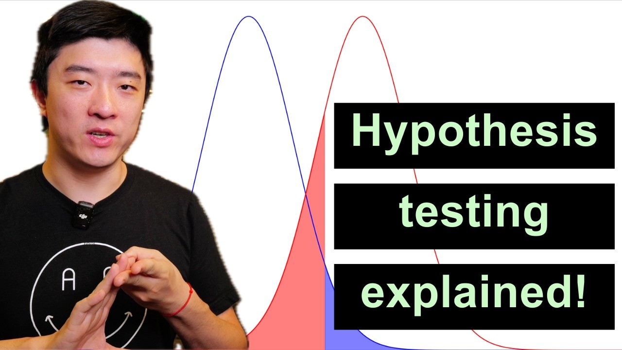
Hypothesis Testing Explained|假设检验详解:Alpha、Beta、Power、MDE与样本量 — 课代表立正

课代表立正

Increase sample size N to reduce standard error, which directly shrinks the minimum detectable effect while preserving target alpha and beta rates.

AI-assisted summary of Hypothesis Testing Explained|假设检验详解:Alpha、Beta、Power、MDE与样本量 — original source. Check the original for full context.

Source published:

Detailed notes

## Background This video was published on YouTube by 课代表立正 on August 29, 2026. According to the page description, it is a visual, formula-light tutorial co-produced with the Statsig data science team that rebuilds hypothesis testing from first principles, disentangling Fisher’s significance testing from the Neyman–Pearson framework. Presented by Yuzheng Sun, PhD, the guide covers fundamental experimentation concepts such as null vs. alternative hypotheses, Type I and Type II errors, statistical power, MDE, and sample size relationships.

## TL;DR Data science content creator Yuzheng Sun breaks down hypothesis testing into an intuitive mental model, addressing common misunderstandings rooted in blended textbook definitions. The walkthrough establishes the null hypothesis, standard error, Type I error (alpha), and critical value thresholds before introducing alternative hypotheses, Type II error (beta), and statistical power. Power is explored through graphical, real-world, and sample size lenses, illustrating how larger sample sizes narrow distribution curves and boost detection capability. Finally, the tutorial defines the Minimum Detectable Effect (MDE) and shows how increasing sample size lowers the MDE, framing the fundamental tradeoffs between speed, scale, and effect size in experimentation.

## Atmosphere & style The video has an educational, grounded, and candid tone, balancing high-level technical rigor with approachable visual explanations. Speaker Yuzheng Sun conveys an empathetic and relatable posture by sharing his own past struggles with textbook definitions, using light self-deprecating humor about data science misconceptions. The dynamic feels like a clear, step-by-step masterclass that demystifies abstract statistical jargon into intuitive physical concepts.

## Key takeaways - [00:00](https://www.youtube.com/watch?v=nCBIotZzPEM&t=0s) Standard textbooks and online sources often present an inconsistent blend of Fisher's p-value significance testing and the Neyman-Pearson decision framework, causing widespread confusion among data scientists. - [02:46](https://www.youtube.com/watch?v=nCBIotZzPEM&t=166s) Under the null hypothesis (H0), which assumes no treatment effect, the sample mean distribution approaches a normal distribution for sufficiently large sample sizes (N ≥ 30) by the Central Limit Theorem. - [02:46](https://www.youtube.com/watch?v=nCBIotZzPEM&t=166s) Standard deviation measures population variability, whereas standard error measures the error of the sample mean and decreases as sample size grows (SE = σ / √N). - [02:46](https://www.youtube.com/watch?v=nCBIotZzPEM&t=166s) Type I error (alpha) is the probability of falsely rejecting the null hypothesis when it is true, and its threshold is set by choosing a critical value. - [06:41](https://www.youtube.com/watch?v=nCBIotZzPEM&t=401s) An alternative hypothesis (H1) represents a theoretical construct; in practice, infinitely many potential alternative hypotheses exist. - [06:41](https://www.youtube.com/watch?v=nCBIotZzPEM&t=401s) Type II error (beta) is the probability of falsely accepting the null hypothesis when a specific alternative hypothesis is actually true. - [09:26](https://www.youtube.com/watch?v=nCBIotZzPEM&t=566s) Statistical power equals 1 - beta and represents the probability of correctly detecting a true treatment effect when one exists. - [09:26](https://www.youtube.com/watch?v=nCBIotZzPEM&t=566s) Increasing sample size shrinks standard error, narrowing distributions and shifting the critical value threshold to significantly increase statistical power. - [11:23](https://www.youtube.com/watch?v=nCBIotZzPEM&t=683s) Minimum Detectable Effect (MDE) is the smallest true treatment effect size that an experimental design can reliably detect at a given power threshold (e.g., 80%). - [11:23](https://www.youtube.com/watch?v=nCBIotZzPEM&t=683s) As sample size increases while holding alpha and beta constant, the Minimum Detectable Effect (MDE) decreases. - [14:26](https://www.youtube.com/watch?v=nCBIotZzPEM&t=866s) Variance reduction techniques like CUPED increase statistical power by reducing population variance (sigma) without needing larger sample sizes. - [14:26](https://www.youtube.com/watch?v=nCBIotZzPEM&t=866s) Practical experimentation requires balancing speed of execution, scale (sample size), and the expected Minimum Detectable Effect (MDE).

## Detailed walkthrough ### [00:00](https://www.youtube.com/watch?v=nCBIotZzPEM&t=0s) Why Hypothesis Testing Matters

Having created over 500 videos as a data science content creator, speaker Yuzheng Sun introduces this tutorial as the first video he would classify as a absolute "must watch" for every data scientist. Hypothesis testing stands out as one of the most fundamental, universal concepts in data science, yet it remains notoriously confusing and widely misunderstood. In fact, Sun jokes that you could easily set up an arbitrage strategy by betting against fellow data scientists on these foundational concepts; most would eagerly take the bet thinking they understand the subject well, only to lose because the underlying principles are so frequently muddled.

The core reason for this widespread confusion is that standard academic textbooks present an inconsistent, frankensteinian blend of two distinct historical frameworks: Ronald Fisher’s $p$-value significance testing and the Neyman–Pearson decision-making framework. Online blog posts and articles only exacerbate the problem by churning out conflicting summaries. Sun candidly admits that despite holding a PhD and working as an experienced data scientist specializing in experimentation, he did not truly understand hypothesis testing at a first-principles level until recently. When he voiced this realization on LinkedIn, it resonated broadly across the professional community. Many data scientists admitted that whenever they need to discuss concepts like $\alpha$, $\beta$, or power, they still have to run back to textbook definitions—a clear signal that they lack a grounded, intuitive mental model.

To solve this, Sun collaborated with the experimentation data science team at Statsig, leveraging their years of hands-on experience helping customers navigate both theoretical and practical experimentation challenges. Through hundreds of client conversations and six thorough revisions, they distilled these concepts down into a visual, formula-light tutorial designed from first principles. The goal is to make these concepts so intuitive that even middle school students can grasp them, while remaining rigorous and technically consistent. The video covers ten core concepts introduced incrementally across four main stages: 1. The null hypothesis, Type I error, $\alpha$, and critical values 2. The alternative hypothesis, Type II error, $\beta$, and statistical power 3. How statistical power scales with sample size 4. The Minimum Detectable Effect (MDE) and its relationship to sample size

- The tutorial synthesizes years of experimentation consulting at Statsig into a formula-free, visual-first framework. - The presentation was rewritten six times to ensure complete technical consistency without sacrificing accessibility.

---

[02:46](https://www.youtube.com/watch?v=nCBIotZzPEM&t=166s) Null Hypothesis, Alpha, and the Critical Value

The walkthrough begins with the baseline case: the null hypothesis ($H_0$), which posits that there is no treatment effect whatsoever. In A/B testing, this is mathematically represented as the difference in means between the treatment and control groups being zero ($\mu_{\text{treatment}} - \mu_{\text{control}} = 0$). By the Central Limit Theorem, the distribution of this sample mean difference approaches a normal distribution as long as the sample size is sufficiently large—where a sample size of $N = 30$ is already enough for the theorem to hold.

At this point, Sun pauses to clarify a vital distinction that often trips people up: standard deviation versus standard error. Standard deviation measures the spread or error of the underlying population distribution. Standard error, on the other hand, measures the error of the sample mean itself. If you draw a single observation from the population, it can land anywhere across the population curve. However, when you draw a sample of observations and average them, the sample mean becomes much tighter and less variable for two reasons: individual observations are more likely to center around the mean, and extreme values on the left and right sides cancel each other out. Consequently, standard error equals standard deviation divided by the square root of the sample size ($\text{SE} = \frac{\sigma}{\sqrt{N}}$). Assuming a simplified null hypothesis where the underlying population distribution has a mean of $0$ and a standard deviation of $1$, a sample size of $N = 30$ yields a standard error of $1 / \sqrt{30} \approx 0.18$.

In hypothesis testing, we draw a sample mean and render a decision: do we accept or reject the null hypothesis? Sun anticipates a classic pedantic objection—addressing whether saying "accept the null hypothesis" rather than "fail to reject the null hypothesis" is technically wrong. He notes that in a simplified setup with only two defined choices, saying "accept the null" is logically sound and far more intuitive for building incremental understanding. Because we operate in a world of random sampling and probability, we can never be 100% certain. Any sample mean along the x-axis can occur by chance, so decision rules must intentionally trade off specific rates of error against the ability to make meaningful discoveries. If a decision rule is made too conservative, you will make zero false positives, but you will also never discover anything new.

To establish a decision rule, we pick a decision threshold along the x-axis known as the critical value. Observed sample means falling below this threshold lead us to accept the null hypothesis, while sample means above it prompt us to reject it. When considering *only* the null hypothesis, there is only one type of mistake possible: a Type I error, which occurs when the null hypothesis is true, but we accidentally reject it due to random noise. The probability of making a Type I error is represented by the area under the tail of the null distribution beyond the critical value, denoted as $\alpha$ (alpha). If an experimenter chooses a standard significance level of $\alpha = 0.05$ (5%), working backward from the sample mean distribution ($\text{SE} \approx 0.18$) yields a critical value threshold of $0.30$.

- **Null Hypothesis ($H_0$):** Assumes zero treatment effect ($\mu_{\text{treatment}} - \mu_{\text{control}} = 0$). - **Central Limit Theorem Rule of Thumb:** $N \ge 30$ is generally sufficient for sample means to approximate a normal distribution. - **Standard Error Formula:** $\text{SE} = \sigma / \sqrt{N}$. With $\sigma = 1$ and $N = 30$, $\text{SE} \approx 0.18$. - **Critical Value Example:** Setting $\alpha = 0.05$ under this specific setup places the decision threshold at a critical value of $0.30$.

---

[06:41](https://www.youtube.com/watch?v=nCBIotZzPEM&t=401s) Alternative Hypothesis, Beta, and Statistical Power

To move beyond avoiding false alarms and actually make scientific discoveries, an alternative hypothesis ($H_1$) must be introduced. Sun highlights a critical insight that standard textbooks rarely emphasize: in reality, there are infinitely many possible alternative hypotheses. An alternative hypothesis is a theoretical construct rather than a single fixed reality; given any observed data point, countless potential alternative distributions could be true with varying probabilities. While the tutorial later addresses how to navigate this infinite set via MDE, it first simplifies the picture by focusing on a single specific alternative hypothesis: one with a true underlying treatment effect mean of $0.5$ and a standard deviation of $1$.

Introducing this specific alternative hypothesis allows the decision rule to be updated. For a sample size of $N = 30$ with a critical value threshold of $0.30$: if the observed sample mean is above $0.30$, we reject $H_0$ and accept $H_1$; if it falls below $0.30$, we accept $H_0$ and reject $H_1$. However, if this alternative hypothesis actually reflects the ground truth, arriving at a sample mean below $0.30$ causes us to mistakenly reject $H_1$. This mistake is called a Type II error—falsely rejecting the alternative hypothesis when it is in fact true. The probability of making a Type II error is designated as $\beta$ (beta).

Sun stresses that $\beta$ is fundamentally tied to the specific alternative hypothesis selected. Shift the assumed alternative distribution left or right, and $\beta$ changes immediately. Three distinct factors dictate the magnitude of $\beta$: 1. The standard error of the alternative distribution 2. The assumed effect size (mean) of the alternative hypothesis 3. The chosen critical value (which is anchored to your target $\alpha$)

If you assume a conservative alternative hypothesis (a mean close to 0), $\beta$ will be very large. If you assume an extreme alternative hypothesis (a mean far to the right), $\beta$ becomes very small. This setup brings us directly to the core tradeoff between making mistakes and making discoveries.

- **Infinite Alternatives:** An infinite number of alternative hypotheses exist theoretically; selecting one allows for explicit decision parameterization. - **Example Alternative Setup:** Mean effect $\mu_1 = 0.5$, $\sigma = 1$. - **Type II Error ($\beta$):** The probability of failing to detect a real effect (falsely rejecting $H_1$ when $H_1$ is true). - **Key Drivers of $\beta$:** Standard error ($\text{SE}$), distance of the alternative mean from zero, and the chosen critical value.

---

[09:26](https://www.youtube.com/watch?v=nCBIotZzPEM&t=566s) Statistical Power in Three Views

Statistical power is the central engine of hypothesis testing, yet textbooks routinely gloss over it with a brief mathematical definition: $\text{Power} = 1 - \beta$. Sun argues that simply knowing this formula is insufficient and breaks power down into three complementary mental models:

1. **The Graphical View:** On the visual distribution plot, power is the shaded area under the alternative hypothesis curve that falls to the *right* of the critical value threshold ($1 - \beta$). It represents the precise probability of correctly accepting a specific alternative hypothesis under your decision rules and assumptions. 2. **The Intuitive Real-World Analogy:** Power measures how capable your test is at detecting a true effect if one exists. Sun illustrates this with a simple real-world example: trying to determine the most popular car manufacturer. If you stand on a corner and observe only a single car, your observation has virtually no statistical power to reveal real brand dominance. But if you survey one million cars across the country, your sample provides immense power to spot true market trends. In short, higher power means a better chance of detecting reality. 3. **The Sample Size & Distribution View:** To see how sample size directly generates power, consider shifting the sample size from $N = 30$ to $N = 100$. Increasing $N$ reduces the standard error ($\text{SE} = \sigma / \sqrt{N}$), causing both the null and alternative probability curves to become significantly narrower and taller. If we maintain our target Type I error rate at $\alpha = 0.05$, this narrower null distribution shifts the critical value threshold much closer to zero. Combining a smaller critical value with a tighter alternative distribution dramatically reduces the area under the left tail ($\beta$), leaving a much larger area to the right. Consequently, the test gains substantial statistical power to catch the effect.

- **Textbook Formula:** $\text{Power} = 1 - \beta$. - **Car Analogy:** Observing 1 car yields low power; observing 1,000,000 cars yields high power to detect true underlying patterns. - **Impact of Increasing Sample Size ($N = 30 \to 100$):** Standard error shrinks $\to$ distributions narrow $\to$ critical value shifts left (for fixed $\alpha$) $\to \beta$ collapses $\to$ statistical power increases significantly.

---

[11:23](https://www.youtube.com/watch?v=nCBIotZzPEM&t=683s) MDE and Sample Size

With the foundational concepts established, Sun resolves the puzzle of how to handle "infinitely many alternative hypotheses" by introducing the Minimum Detectable Effect (MDE). Because alternative hypotheses are theoretical constructs, an experimenter can evaluate any hypothetical mean along the axis. In a sample of $N = 30$ with $\alpha = 0.05$, an alternative hypothesis centered at $\mu = 0.50$ yields $\beta = 0.14$ (Power = $86\%$). If we evaluate a more conservative alternative centered closer at $\mu = 0.45$, the overlap with the critical value increases, raising $\beta$ to $0.20$ (Power = $80\%$).

Because practitioners always desire higher power to detect real improvements, any true effect size situated to the *right* of this $\mu = 0.45$ threshold will be detected with *even greater* power (lower $\beta$). Therefore, $0.45$ represents the Minimum Detectable Effect—the smallest true treatment effect size that the experimental design can reliably catch at the required power threshold (e.g., $80\%$).

To tie every concept in the tutorial together, Sun walks through how MDE scales when sample size increases from $N = 30$ to $N = 100$ while holding both $\alpha$ (5%) and $\beta$ (20%) strictly constant: - As $N$ grows from $30$ to $100$, the standard error contracts, narrowing the sampling distributions. - Holding $\alpha = 0.05$ pushes the critical value threshold to the left. - Holding $\beta = 0.20$ (80% power) forces the required alternative distribution to slide closer to the null mean. - As a direct result, the MDE drops from $0.45$ down to $0.25$.

This demonstrates the core rule of experimental design: **as sample size increases, MDE decreases.** A larger sample size allows an experiment to detect much smaller, subtle nuances. Conversely, if a feature change produces a massive treatment effect, an organization does not need billions of users or huge sample sizes to validate it—a small sample size will easily detect a large effect with high statistical power.

- **MDE Definition:** The smallest true effect size ($\mu_1$) that can be detected for a given $\alpha$, $\beta$, and sample size $N$. - **MDE Scaling Example:** Increasing sample size from $N = 30$ to $N = 100$ (with fixed $\alpha = 0.05, \beta = 0.20$) reduces the MDE from $0.45$ to $0.25$. - **Practical Implication:** Companies without massive user bases can still run reliable A/B tests, provided their product changes produce large impact sizes.

---

[14:26](https://www.youtube.com/watch?v=nCBIotZzPEM&t=866s) Key Takeaways and Practical Applications

Sun concludes by emphasizing that a deep, intuitive mastery of statistical power is the prerequisite foundation for almost every advanced topic in A/B testing and experimentation. Without a solid first-principles understanding of power, advanced techniques remain abstract and prone to misapplication.

He highlights several real-world experimentation challenges that tie directly back to power: - **Variance Reduction Techniques (e.g., CUPED):** While the tutorial held standard deviation constant at $\sigma = 1$, real-world data is noisy. Advanced techniques like CUPED reduce variance ($\sigma$), which shrinks the standard error and boosts statistical power without requiring larger user samples. - **Sequential Testing & Early Peeking:** Running underpowered tests or continually checking results without adjusting thresholds leads to false discoveries and poor business decisions. - **The Experimentation Tradeoff:** Practical A/B testing is a constant balancing act between three competing forces: execution speed, scale (sample size), and the expected minimum effect size you aim to detect.

Sun closes by encouraging viewers to use this visual mental model when explaining experimentation trade-offs to business stakeholders, saving hours of confusion down the road.

- **CUPED & Variance Reduction:** Reduces $\sigma$ directly, shrinking standard error to increase statistical power without extending runtime. - **The Triad of Experimentation:** Speed of iteration, sample scale, and target MDE are inherently linked through statistical power.

<ElicitationsGroup message="Where would you like to go next with these statistical concepts?"> <Elicitation label="Explain how CUPED reduces variance mathematically" query="Explain how CUPED (Controlled-Experiments Using Pre-Experiment Data) reduces variance and increases statistical power in A/B testing."/> <Elicitation label="Compare Fisher vs. Neyman-Pearson frameworks" query="Break down the historical and theoretical differences between Ronald Fisher's p-value significance testing and the Neyman-Pearson decision framework."/> <Elicitation label="Calculate required sample size for a custom A/B test" query="How do I calculate the required sample size for an A/B test given a target baseline conversion rate, MDE, alpha, and power?"/> </ElicitationsGroup>

## Notable quotes > [00:00](https://www.youtube.com/watch?v=nCBIotZzPEM&t=0s) Hypothesis testing stands out as one of the most fundamental, universal concepts in data science, yet it remains notoriously confusing and widely misunderstood. — Yuzheng Sun

> [00:00](https://www.youtube.com/watch?v=nCBIotZzPEM&t=0s) you could easily set up an arbitrage strategy by betting against fellow data scientists on these foundational concepts — Yuzheng Sun

> [00:00](https://www.youtube.com/watch?v=nCBIotZzPEM&t=0s) standard academic textbooks present an inconsistent, frankensteinian blend of two distinct historical frameworks: Ronald Fisher’s p-value significance testing and the Neyman–Pearson decision-making framework. — Yuzheng Sun

> [02:46](https://www.youtube.com/watch?v=nCBIotZzPEM&t=166s) Standard deviation measures the spread or error of the underlying population distribution. Standard error, on the other hand, measures the error of the sample mean itself. — Yuzheng Sun

> [02:46](https://www.youtube.com/watch?v=nCBIotZzPEM&t=166s) Any sample mean along the x-axis can occur by chance, so decision rules must intentionally trade off specific rates of error against the ability to make meaningful discoveries. — Yuzheng Sun

> [06:41](https://www.youtube.com/watch?v=nCBIotZzPEM&t=401s) in reality, there are infinitely many possible alternative hypotheses. — Yuzheng Sun

> [06:41](https://www.youtube.com/watch?v=nCBIotZzPEM&t=401s) Type II error—falsely rejecting the alternative hypothesis when it is in fact true. — Yuzheng Sun

> [09:26](https://www.youtube.com/watch?v=nCBIotZzPEM&t=566s) Statistical power is the central engine of hypothesis testing, yet textbooks routinely gloss over it with a brief mathematical definition — Yuzheng Sun

> [09:26](https://www.youtube.com/watch?v=nCBIotZzPEM&t=566s) If you stand on a corner and observe only a single car, your observation has virtually no statistical power to reveal real brand dominance. But if you survey one million cars across the country, your sample provides immense power to spot true market trends. — Yuzheng Sun

> [11:23](https://www.youtube.com/watch?v=nCBIotZzPEM&t=683s) as sample size increases, MDE decreases. — Yuzheng Sun

> [11:23](https://www.youtube.com/watch?v=nCBIotZzPEM&t=683s) a small sample size will easily detect a large effect with high statistical power. — Yuzheng Sun

> [14:26](https://www.youtube.com/watch?v=nCBIotZzPEM&t=866s) Practical A/B testing is a constant balancing act between three competing forces: execution speed, scale (sample size), and the expected minimum effect size you aim to detect. — Yuzheng Sun

## Mentioned Yuzheng Sun, Statsig, Ronald Fisher, Jerzy Neyman, Egon Pearson, YouTube, LinkedIn, CUPED

[Source](https://www.youtube.com/watch?v=nCBIotZzPEM)

中文简报

Statsig团队可视化功效权衡以修复A/B测试缺陷 增加样本量N以降低标准误,从而在保持目标alpha和beta率的同时直接缩小最小可检测效应。 数据科学内容创作者Yuzheng Sun将假设检验拆解为直观的心智模型,化解了源于教科书中混合定义的常见误解。该解析在引入备择假设、第二类错误(beta)和统计功效之前,首先阐明了原假设、标准误、第一类错误(alpha)以及临界值阈值。随后从图表、现实场景和样本量等视角对统计功效进行了探讨,说明了更大的样本量如何收窄分布曲线并提高检测能力。最后,教程定义了最小可检测效应(MDE),展示了增加样本量如何降低MDE,并系统呈现了实验中速度、规模与效应量之间的核心权衡。 传统教科书和网络资料常将 Fisher 的显著性检验与 Neyman–Pearson 决策框架混淆,导致数据科学家普遍缺乏对假设检验底层逻辑的直观理解。 (0:00) 在零假设(H0)下,根据中心极限定理,当样本量充分(N ≥ 30)时样本均值趋近于正态分布;标准误差随样本量增加而缩小(SE = σ / √N),而第一类错误率(alpha)则决定了拒绝零假设的临界值阈值。 (2:46) 备择假设在理论上存在无数种可能,其设定的均值、标准误差与临界值共同决定了第二类错误率(beta);统计功效(Power = 1 - beta)表示在真实效应存在时正确检测出该效应的概率。 (6:41) 最小可检测效应(MDE)是实验在既定功效下能可靠识别的最小真实效应;增加样本量会压缩标准误差并使临界值向中心移动,从而显著降低 MDE 并大幅提高统计功效。 (11:23) 对统计功效的直观掌握是理解 CUPED 等方差缩减技术及避免过早窥探(Peeking)的基础,企业在 A/B 测试中需持续在迭代速度、样本规模与目标 MDE 之间权衡取舍。 (14:26)

Reading summary

Data science educator Yuzheng Sun, in collaboration with experimentation platform Statsig, outlines a first-principles, visual framework to demystify hypothesis testing by framing decision thresholds, error rates, and statistical power as interdependent trade-offs. The Theoretical Roots of Practitioner Confusion (0:00) Hypothesis testing remains widely misunderstood across data science because standard academic curricula merge two conflicting historical schools: Ronald Fisher's p-value significance testing and the Neyman–Pearson decision-making framework. This hybrid presentation leaves practitioners without an intuitive mental model, forcing experienced data scientists to repeatedly consult textbook formulas for basic concepts like alpha, beta, and statistical power. To establish a grounded understanding, Sun and Statsig distilled years of experimentation consulting into a visual, formula-light model revised six times for conceptual consistency. Null Hypothesis, Standard Error, and Type I Error (2:46) The baseline of an A/B test is the null hypothesis (H₀), which assumes zero treatment effect (mean treatment difference equals zero). Under the Central Limit Theorem, sample mean differences approximate a normal distribution when sample size reaches roughly N ≥ 30. Standard error (SE = σ / √N) reflects the variability of the sample mean rather than the population spread (σ), shrinking as extreme sample observations cancel each other out. In a standardized scenario (σ = 1, N = 30), standard error equals approximately 0.18. Because probability distributions mean any sample outcome can occur by chance, decision rules require a critical value threshold along the horizontal axis. Sample means falling beyond this threshold trigger rejection of the null hypothesis. The probability of falsely rejecting a true null hypothesis due to random noise is the Type I error (α). Setting a standard significance level of α = 0.05 on a sample distribution with SE ≈ 0.18 establishes a critical value decision threshold of 0.30. Alternative Hypotheses, Beta, and Three Dimensions of Power (6:41) In reality, an infinite number of potential alternative hypotheses (H₁) could be true. Specifying a theoretical alternative hypothesis—such as a true treatment effect of μ₁ = 0.5 with σ = 1—allows experimenters to measure Type II error (β), the probability of mistakenly accepting the null hypothesis when an effect actually exists. The magnitude of β shifts based on the standard error, the chosen critical value, and the distance between the alternative mean and zero. Statistical power, formally defined as 1 - β, represents the probability of correctly detecting a real effect. Sun breaks power into three complementary models: graphically, it is the area under the alternative distribution curve falling to the right of the critical threshold; intuitively, it mirrors the difference between sampling one car versus one million cars to identify true brand dominance; and distributionally, increasing sample size (e.g., N = 30 to N = 100) contracts standard errors, narrows both curves, pulls the critical value toward zero for a fixed α, and collapses β, thereby substantially raising power. Minimum Detectable Effect and Sample Size Dynamics (11:23) The Minimum Detectable Effect (MDE) resolves the challenge of evaluating infinite alternative hypotheses by identifying the smallest true effect size that an experiment can reliably catch at a prescribed power threshold (such as 80%, where β = 0.20). In an experiment with N = 30 and α = 0.05, a hypothesized effect of μ = 0.50 yields 86% power (β = 0.14), while a smaller effect of μ = 0.45 yields 80% power (β = 0.20), establishing 0.45 as the design's MDE. Increasing sample size directly lowers MDE. Expanding from N = 30 to N = 100 while maintaining α = 0.05 and β = 0.20 narrows sampling distributions and reduces the MDE from 0.45 to 0.25. This dynamic demonstrates that while detecting subtle product nuances requires large sample sizes, organizations do not need massive user volume to validate features that yield large impact sizes. Advanced Experimentation and Operational Trade-Offs (14:26) Mastery of statistical power is essential for applying advanced experimentation techniques. Variance reduction methods such as CUPED directly decrease standard deviation (σ), compressing standard error and increasing statistical power without lengthening test runtimes or recruiting more users. Conversely, failing to account for statistical power leads to flawed practices such as early peeking and underpowered testing, which inflate false discoveries. Practical A/B testing ultimately operates as a perpetual balancing act among iteration velocity, available sample scale, and the target minimum effect size. Sun concludes that grounding experimentation in visual, first-principles concepts enables practitioners to navigate advanced methodologies and clearly communicate testing constraints to business stakeholders, though every experiment remains fundamentally bounded by trade-offs among execution speed, sample size, and effect resolution.

精炼阅读摘要

主讲人Yuzheng Sun联合实验平台Statsig指出,数据科学界对假设检验的长期困惑源于经典教材割裂混合了费舍尔与奈曼-皮尔逊两种统计框架;通过建立第一性原理与可视化模型,实验者能够直观理解α、β、统计功效与MDE之间的内在权衡,为A/B测试设计提供科学依据。 理论混杂与第一性原理认知缺失 (0:00) Sun指出,假设检验虽然是数据科学中最通用的基础工具,却普遍存在理解混乱。这种现象的核心原因在于主流学术教材将罗纳德·费舍尔(Ronald Fisher)的p值显著性检验与奈曼-皮尔逊(Neyman–Pearson)的决策框架拼凑在一起,造成了逻辑上的割裂与自相矛盾,导致许多拥有博士学位或资深实验经验的数据科学家仍需频繁查阅教科书定义。 针对这一痛点,Sun与Statsig团队结合大量企业客户的实验咨询经验,历经六次修订,试图剥离繁琐公式,仅通过图形与第一性原理还原假设检验的本质。该框架将复杂的推断过程分解为零假设、备择假设、样本量缩放以及最小可检测效应(MDE)四个循序渐进的阶段,旨在建立一套中学生也能听懂、同时保持数学严谨性的心智模型。 零假设基准、标准误与第一类错误 (2:46) 检验从零假设(H0)展开,其基准设定为处理组与对照组之间无处理效应(差值为0)。根据中心极限定理,只要样本量达到N=30,样本均值的抽样分布即近似于正态分布。Sun在此明确区分了总体标准差与样本均值的标准误(SE = σ / √N):单次观测值的离散度由标准差衡量,而抽样均值由于正负极值相互抵消,其变异度显著更小。在总体标准差为1、样本量为30的基准设定下,标准误约为0.18。 在存在随机抽样波动的情况下,实验必须设定决策阈值(即临界值)来决定接受或拒绝零假设。当只考虑零假设时,决策可能犯的唯一错误是第一类错误(伪阳性),即零假设本为真却被随机噪声误判拒绝。该错误发生的概率对应于临界值右侧的尾部面积,记为α。若将显著性水平设定为常规的α = 0.05,在标准误约为0.18的分布下,推算出的临界值阈值约为0.30。 备择假设、第二类错误与功效模型 (6:41) 为了做出真正的发现,实验必须引入备择假设(H1)。Sun强调,现实中备择假设在理论上存在无穷多个,它不是单一事实而是人为构建的假设分布。设定一个均值效应为0.5、标准差为1的具体备择分布,若样本均值低于0.30的临界值,决策规则将判定接受零假设,从而错误拒绝了真实的备择假设,这种伪阴性错误被称为第二类错误,其发生概率记为β。β的数值严格依赖于所选备择假设的均值位置、标准误以及由α决定的临界值。 统计功效定义为1 - β,即在效应真实存在时正确检出该效应的概率。Sun提出了三维理解视角:第一是图形视角,功效即备择分布落在临界值右侧的阴影面积;第二是直觉视角,在街头观察1辆车无法推断汽车市场份额,而调研100万辆车则具备极高功效;第三是分布收缩视角,当样本量由30提升至100时,标准误减小使曲线变窄变高,在α固定的前提下临界值向左平移,从而急剧压缩β的面积,显著提升统计功效。 MDE收缩机制与实验权衡策略 (11:23) 最小可检测效应(MDE)解决了“备择假设有无穷多个”的难题。在给定的显著性水平(如α = 0.05)和目标功效(如80%,对应β = 0.20)下,MDE代表该实验设计所能可靠探测到的最小真实效应量。在N = 30的设定下,能够达到80%功效的备择分布均值落在0.45处,因此0.45即为此配置下的MDE。 当样本量扩大至N = 100而保持α与β不变时,标准误的收缩使临界值左移,所需的备择假设中心也随之向零点靠近,MDE相应从0.45下降至0.25。这一规律证明:样本量越大,实验越能捕捉极其微弱的改动;反之,若业务变更能产生巨大突破,即使在小样本量下也能以高功效快速检出。Sun进一步引申,实践中的CUPED等方差缩减技术本质上是通过降低总体标准差σ来收缩标准误,进而提升功效,整个A/B测试是一场在研发速度、样本规模与目标MDE之间的平衡艺术。 Sun总结认为,建立直观的统计功效心智模型是避免日常实验误判与应对进阶测试(如连续监控、方差缩减)的前提;这一模型能够帮助数据科学家向业务方清晰阐明实验成本与检测灵敏度之间的工程权衡。

Detailed notes — zh

## Background 该内容由 YouTube 频道“课代表立正”(主讲人为孙玉铮博士,Yuzheng Sun)于 2026 年 9 月 5 日发布。视频基于作者与 Statsig 数据科学团队历经六版迭代的工业界实践沉淀,旨在打破传统教科书中费舍尔显著性检验与内曼-皮尔逊决策框架的混淆,通过直观无公式的可视化图示从第一性原理重构假设检验体系。 ## TL;DR 视频系统性梳理了数据科学中极易被误解的假设检验底层逻辑。内容从原假设与备择假设的设定切入,严格区分了总体标准差与样本均值标准误的物理差异,并结合中心极限定理阐明了基于临界值的决策机制。随后,主讲人深入剖析了第一类错误(Alpha)、第二类错误(Beta)以及统计功效(Power)的三维几何与业务本质,最终揭示了最小可检测效应(MDE)与样本量的联动规律,为企业进行高效、精准的 A/B 测试决策提供了完备的认知框架。 ## Atmosphere & style 整期视频呈现出一种返璞归真、通透且极具说服力的硬核教学氛围。主讲人以资深从业者兼学者的坦诚视角,撕下统计学公式的晦涩外衣,用平实质朴的语言直击行业长期存在的认知痛点。讲解节奏循序渐进、逻辑环环相扣,配合清晰直观的几何推演,给观众带来一种“困扰多年的统计迷思终于被彻底融会贯通”的豁然开朗感。 ## Bulletin - [00:00](https://www.youtube.com/watch?v=nCBIotZzPEM&t=0s) 统计学教科书常将费舍尔的显著性检验与内曼-皮尔逊决策框架机械拼凑,导致数据科学家容易对原假设、备择假设等核心定义产生认知混乱。 - [11:23](https://www.youtube.com/watch?v=nCBIotZzPEM&t=683s) 现实中备择假设在理论上存在无穷多个,最小可检测效应(MDE)本质上是在给定 Alpha 和 Beta(功效通常设为 80%)阈值下反推得到的备择假设效应量检测下限。 - [13:16](https://www.youtube.com/watch?v=nCBIotZzPEM&t=796s) 样本量增加会收窄样本均值标准误并压低 MDE;这一规律意味着微小效应依赖大流量捕捉,而显著的业务强信号在中小流量下也能被高置信度检出。 - [14:26](https://www.youtube.com/watch?v=nCBIotZzPEM&t=866s) 工业界主流实验技巧如 CUPED 方差缩减与序贯检验均紧密围绕统计功效(Power)展开,以此平衡实验迭代速度、流量规模与预期效应。 ## Key takeaways - [00:00](https://www.youtube.com/watch?v=nCBIotZzPEM&t=0s) 假设检验认知混乱的核心根源在于大学教科书将费舍尔(Fisher)的显著性检验体系与内曼-皮尔逊(Neyman–Pearson)决策框架杂糅拼接。 - [02:46](https://www.youtube.com/watch?v=nCBIotZzPEM&t=166s) 必须严格区分标准差与标准误:标准差衡量真实总体的离散度,而标准误(SE)衡量多次抽样均值的离散度,并随样本量增大按根号关系衰减收窄。 - [02:46](https://www.youtube.com/watch?v=nCBIotZzPEM&t=166s) 第一类错误(Type I Error / Alpha)是原假设为真时错误拒绝原假设的概率,由设定的拒绝域临界值位置直接决定。 - [02:46](https://www.youtube.com/watch?v=nCBIotZzPEM&t=166s) 假设检验本质上是在“控制错误概率”与“保留业务发现能力”之间权衡,如果决策门槛定得无限苛刻,将导致永远无法获得业务新洞察。 - [06:41](https://www.youtube.com/watch?v=nCBIotZzPEM&t=401s) 备择假设并非现实中客观唯一的物理实体,而是理论构建,在现实观测数据背后理论上存在无数个潜在备择假设。 - [06:41](https://www.youtube.com/watch?v=nCBIotZzPEM&t=401s) 第二类错误(Type II Error / Beta)衡量当某个特定备择假设为真时漏报该效果的概率,受临界值、备择假设均值及标准误共同影响。 - [09:26](https://www.youtube.com/watch?v=nCBIotZzPEM&t=566s) 统计功效(Power / 1 - Beta)即在备择假设为真时正确检出该效应的概率,代表了实验设计探测真实效应的敏锐度与确定性。 - [11:23](https://www.youtube.com/watch?v=nCBIotZzPEM&t=683s) MDE 并非凭空设定的指标,而是在固定总体分布、原假设、Alpha 与最低功效门槛(Beta 通常为 20%)前提下反推的最小可检出均值。 - [13:16](https://www.youtube.com/watch?v=nCBIotZzPEM&t=796s) 样本量增加会显著缩小标准误,导致 MDE 相应下降;这使得大样本能探测极微小改动,而具有大效应的改版无需海量流量即可验证。 - [14:26](https://www.youtube.com/watch?v=nCBIotZzPEM&t=866s) CUPED 等方差缩减技术通过数学方法降低方差以放大功效,避免实验因功效不足(Underpowered)诱发假阳性误判。 ## Detailed walkthrough ### [00:00](https://www.youtube.com/watch?v=nCBIotZzPEM&t=0s) 假设检验的认知陷阱与第一性原理重构 作为一名创作了 500 多期视频的数据科学博主,主讲人孙玉铮博士(Yuzheng Sun)直言,这是他制作的所有内容中第一期真正称得上“所有数据科学家必看”的视频。假设检验是数据科学中最基础、最通用的核心支柱,但同时也是最令人困惑、最常被误解的概念。这种混淆程度甚至高到可以在现实中拿它来与数据科学家打赌赚钱——由于这一概念被默认为“从业者理应精通的常识”,大部分数据科学家都会毫不犹豫地接下赌局,但最终往往会因为认知模糊而输掉赌局。 之所以会出现这种普遍的认知混乱,根本原因在于大学统计学教科书在编撰时,将两种本质不同的框架杂糅在了一起:一种是源于费舍尔(Ronald Fisher)的显著性检验与 p 值体系,另一种则是内曼-皮尔逊(Neyman–Pearson)的决策与假设检验框架。网络上大量参差不齐的技术文章更是加剧了这种割裂。主讲人坦白道,即便自己拥有博士学位,且长期深耕于实验科学与 A/B 测试领域,也是直到最近几年才真正从第一性原理上彻底融会贯通。当他在 LinkedIn 上分享这一心路历程时,引发了行业内无数资深数据科学家的强烈共鸣:大家发现自己每次讨论技术定义时,都不得不翻出教科书重新核对公式,这恰恰说明大家并未真正从本质上吃透它。 本期内容的诞生源于 Statsig 数据科学团队多年来在工业界服务客户的深厚积累。团队面对过形形色色的实验挑战,既要辅导毫无经验的初学者,也要与资深的增长架构师过招,始终在晦涩的统计理论与真实业务决策之间寻找平衡。团队将数年间与客户进行的数百次深度沟通沉淀为认知模型,历经六版彻底推倒重来的打磨,最终凝练成这一套完全不依赖复杂公式、仅凭直观图示与第一性原理构建的教学框架。整个讲解将循序渐进地拆解 10 个核心概念,无论是中学生还是资深工程师都能无障碍理解。 - **教科书矛盾根源**:机械拼凑费舍尔的 p 值显著性检验与内曼-皮尔逊决策框架,导致定义割裂。 - **十个核心知识点路径**: 1. 原假设(Null Hypothesis) 2. 第一类错误(Type I Error) 3. 显著性水平(Alpha, $\alpha$) 4. 临界值(Critical Value) 5. 备择假设(Alternative Hypothesis) 6. 第二类错误(Type II Error) 7. Beta($\beta$) 8. 统计功效(Statistical Power) 9. 最小可检测效应(MDE) 10. 样本量与功效的动态演变 --- ### [02:46](https://www.youtube.com/watch?v=nCBIotZzPEM&t=166s) 原假设、标准误与决策临界值(Alpha) 构建假设检验的第一步是确立原假设($H_0$),并厘清统计学中最易混淆的一对术语:标准差(Standard Deviation)与标准误(Standard Error)。原假设的业务本质是“实验组没有任何处理效应(Treatment Effect)”,通常表现为实验组均值与对照组均值之差为零。根据中心极限定理(CLT),只要样本量充分大(通常经验法则中样本量达到 30 即可),均值差值的底层抽样分布就会趋近于正态分布。 在这里必须严格区分底层分布与样本均值分布的误差度量:底层真实总体的离散程度称为**标准差**;而由多次抽样计算得出的样本均值的离散程度,则被称为**标准误**。如果我们只从总体中抽取单次观测值,其结果可能散落在坐标轴的任意位置;但若抽取大量样本并计算样本均值,由于均值向中心集中的概率更高,且样本间的正负偏差会相互抵消,样本均值的误差分布必定显著收窄。标准误在数学上等于标准差除以样本量的平方根($SE = \sigma / \sqrt{n}$)。假设原假设的底层分布均值为 0、标准差为 1,当抽取 30 个样本时,样本均值的标准误约为 $1 / \sqrt{30} \approx 0.18$。 ```mermaid flowchart TD accTitle: 抽样分布与决策机制流程图 accDescr: 展示从总体分布到计算标准误,再由临界值划分接受与拒绝原假设的决策流程 subgraph Dist["误差与分布演变"] A["总体分布: 均值=0, 标准差 σ=1"] --> B["抽取样本: n = 30"] B --> C["样本均值分布: 标准误 SE ≈ 0.18"] end subgraph Decision["决策边界与第一类错误"] C --> D{"样本均值 vs 临界值 0.30"} D -- "样本均值 > 0.30" --> E["拒绝原假设 (Reject H₀)"] D -- "样本均值 ≤ 0.30" --> F["接受原假设 (Accept H₀)"] E -. "若真实无效应 (概率 5%)".-> G["第一类错误 (Type I Error / Alpha)"] end ``` 假设检验的终极目标是基于观察到的样本做出业务决策:到底是有效果还是没效果?是该拒绝原假设还是接受原假设?针对部分统计学原教旨主义者常纠结的“只能说未能拒绝原假设(Fail to reject $H_0$),不能说接受原假设(Accept $H_0$)”,主讲人明确指出,在严格设定的二元假设决策框架下,“接受原假设”不仅在工程上完全成立,也是更直观、不易出错的概念表述。 因为现实处于概率世界,X 轴上的任何样本结果都有可能发生,我们永远无法做出 100% 绝对正确的判断。如果把决策门槛定得无限苛刻,固然永远不会犯错,但同时也意味着永远无法获得业务新发现。因此,假设检验的核心在于平衡“错误容忍度”与“业务发现能力”。我们需要在分布曲线上切出一道阈值,高于该阈值则拒绝原假设,低于该阈值则接受原假设,这个阈值就是**临界值(Critical Value)**。在仅引入原假设的阶段,我们只会犯一种错误:当原假设为真时却错误地拒绝了它,这就是**第一类错误(Type I Error)**。曲线上方超出临界值的尾部概率面积即为 **$\alpha$(Alpha)**。若我们将容许的 $\alpha$ 设定为 5%(0.05),在 $SE \approx 0.18$ 的正态分布下,经计算对应的临界值约为 0.30。此时决策规则极为清晰:抽取 30 个样本,若样本均值超过 0.30 则拒绝原假设,反之则接受原假设。 - **样本均值收敛机制**:样本量增大使得均值标准误收窄,核心原因在于中心趋势概率增大以及极端偏离值正负相互抵消。 - **临界值决策点**:在 $\alpha = 0.05$、$n = 30$ 条件下,拒绝域切点临界值为 0.30。 - **探索与谨慎的权衡**:"If we set our decision rule to be extreme, we won't make mistakes, but we won't make discoveries either."(如果我们把决策规则定得极其极端,我们确实不会犯错,但也永远无法做出任何发现。) --- ### [06:41](https://www.youtube.com/watch?v=nCBIotZzPEM&t=401s) 备择假设的理论虚构、Beta 与第二类错误 明确了原假设的防线后,为了实现业务上的突破与发现,必须引入备择假设(Alternative Hypothesis, $H_1$)。在此处,绝大多数教科书都忽略了一个引发长期困惑的关键前提:**在现实世界中,备择假设在理论上存在无穷多个**。备择假设并非客观存在的单一实体,而是一种理论构建(Theoretical Construct)。对任意观测数据而言,背后都可能对应着无数个不同均值和不同方差的潜在备择假设,每一个都以一定的概率成立。 为了打破这种无穷维度的复杂性,必须人为挑选一个特定的备择假设来进行推演。假设我们设定一个具体的备择假设分布:真实均值为 0.5,底层标准差同样为 1。将其与原假设并列于坐标轴上,由于红色的备择假设曲线的引入,二元决策体系得以完整闭环: 1. 若样本均值大于 0.30:拒绝原假设,同时**接受该备择假设**; 2. 若样本均值小于 0.30:接受原假设,同时**拒绝该备择假设**。 此时便不可避免地引入了**第二类错误(Type II Error)**:当该备择假设客观为真(即策略确实有正向效果)时,我们却因为样本均值未突破临界值 0.30,而错误地拒绝了备择假设。犯第二类错误的概率被定义为 **$\beta$(Beta)**。 | 决策要素 | 第一类错误(Type I Error / $\alpha$) | 第二类错误(Type II Error / $\beta$) | |:--- |:--- |:--- | | **真实真实情况** | 原假设为真(无效果) | 备择假设为真(有效果) | | **实验决策结果** | 错误地拒绝原假设(误报为有效) | 错误地拒绝备择假设(漏报真实效果) | | **图表几何表征** | 原假设分布在临界值右侧的尾部面积 | 备择假设分布在临界值左侧的尾部面积 | | **影响决定因素** | 临界值的位置选取 | 临界值、备择假设的均值大小、备择假设的标准误 | 主讲人特别强调,$\beta$ 本质上衡量的是“拒绝某一个**特定**备择假设的概率”。一旦平移或更改所假设的备择分布均值,$\beta$ 的大小就会剧烈变动。影响 $\beta$ 的核心变量有三项:备择假设的标准误、备择假设设定的均值大小、以及由 $\alpha$ 所决定的临界值位置。如果将备择假设设定得过于保守(均值非常接近 0),$\beta$ 就会极其庞大(极易漏报);如果备择假设设定得非常激进偏向右侧极端值,$\beta$ 就会迅速缩减。 --- ### [09:26](https://www.youtube.com/watch?v=nCBIotZzPEM&t=566s) 统计功效(Power)的三维透视与样本量跃迁 在明晰了 $\beta$ 的几何与逻辑定义后,统计检验的核心王牌——**统计功效(Statistical Power)**便水到渠成。标准教科书通常草率地将功效定义为 $1 - \beta$,随后便戛然而止,这给初学者留下了巨大的认知鸿沟:“到底为什么是 $1 - \beta$?功效在现实业务中究竟意味着什么?” 为了彻底解构这个关键概念,主讲人从三个由浅入深的维度进行剖析: - **维度一(几何与概率定义)**:在既定的假设设定与临界决策规则下,当特定的备择假设为真时,我们**正确识别并接受该备择假设的概率**,在图表上即为备择假设分布在临界值右侧的广阔面积。 - **维度二(生活化常识比喻)**:统计功效衡量的是实验设计探测真实效应的敏锐度与确定性。例如想要通过街头观察来判定哪家汽车制造商在当地最受欢迎,如果仅在路口看 1 辆车的品牌,这种观测的探测功效近乎于零,充满随机噪点;但如果系统性记录了 100 万辆汽车的品牌分布,样本就具备了极其强大的功效。"A powerful test means I have a higher chance of detecting a true effect."(一个高功效的检验,意味着当真实效应存在时,我们有极高的概率抓住它。) - **维度三(样本量驱动的动态分布)**:当把抽象定义与样本量直观关联起来时,功效的几何形态便呈现出动态收缩。将实验样本量由 30 人提升至 100 人,分母中的 $\sqrt{n}$ 增大直接驱使均值标准误变小,原假设与备择假设两条正态分布曲线的形态双双变瘦、变窄。这种分布的集中压缩,直接拉开了两座钟形曲线之间的相对重叠距离,为后续在不牺牲 $\alpha$ 的前提下大幅压低 $\beta$、提升功效奠定了物理基础。 ### [10:51](https://www.youtube.com/watch?v=nCBIotZzPEM&t=651s) 检验功效与备择假设的选择 当我们将显著性水平 $\alpha$(Alpha)设定在 5% 时,它所对应的拒绝域临界值(Critical Value)会相应变小。临界值更小,再加上增加样本量所带来的更小标准误(Standard Error),两者结合直接带来了显著提升的统计功效(Statistical Power)。这意味着对于同一个既定的备择假设(Alternative Hypothesis),研究者犯第二类错误(Type II Error,即未能正确识别出真实存在的差异)的概率大幅降低,从而拥有极其充沛的功效来捕捉到这一效应。至此,备择假设、$\beta$(Beta,第二类错误率)以及统计功效($1-\beta$)之间的几何与概率关联已经彻底明朗。 ```mermaid flowchart LR accTitle: 统计功效与参数联动关系 accDescr: 展示样本量增加如何通过缩小标准误和降低临界值,最终提升检验功效并压低第二类错误。 subgraph S1["样本特征调整"] A["增加样本量 N"] --> B["标准误 SE 缩小"] end subgraph S2["决策边界与功效"] C["固定显著性水平 α = 5%"] --> D["临界值 Critical Value 减小"] B --> E["功效 Power 显著提升"] D --> E E --> F["第二类错误 β 大幅降低"] end ``` ### [11:23](https://www.youtube.com/watch?v=nCBIotZzPEM&t=683s) 最小可检测效应(MDE)的本质定义 在现实世界中,原假设通常只有一个(例如效应为零),但备择假设在理论构想上却有无数个。为了在无穷无尽的可能性中锁定基准,统计学引入了“最小可检测效应”(Minimum Detectable Effect, MDE)的概念。如果用一条红色虚线标出备择假设的均值分布,当假定该均值为 0.5 时,它可能对应 14% 的 $\beta$ 和 86% 的统计功效。但若在相同的样本条件下,我们将检验的目标功效基准定在更为通用的 80%(即容忍 20% 的 $\beta$),就必须切换到一个更为保守的备择假设。经测算,当备择假设的真实均值为 0.45 时,刚好对应 20% 的 $\beta$。这是一个检测难度更高的保守假设,犯第二类错误的风险也随之上升到了预设上限。 在统计推断中,追求更高的统计功效几乎是唯一的铁律,因为越高的功效代表着越高概率捕捉到真实存在的业务提升。任何位于 0.45 右侧的备择假设,都属于“更优质、更容易被检出”的备择假设,因为它们距离原假设更远,对应的 $\beta$ 更小,功效更高。因此,MDE 的严谨定义应当是:在给定的底层数据分布假设、给定的原假设、给定的显著性水平 $\alpha$(用于划定临界值)以及预设的 $\beta$(决定了最低功效门槛)这四大前提下,系统能够可靠检测出的备择假设均值的最小值。任何高于该最小阈值的真实效应,实验不仅能够稳稳捕捉,而且会拥有高于预设基准的检验功效。 - **均值 0.5 的备择假设**:对应 $\beta = 14\%$,统计功效 $\text{Power} = 86\%$。 - **均值 0.45 的备择假设**:对应 $\beta = 20\%$,统计功效 $\text{Power} = 80\%$,构成了该设定下的临界效应。 - **MDE 的本质判定**:它并非凭空捏造的指标,而是以预设的 $\alpha$ 与 $\beta$ 容忍度为标尺,反推得到的效应量检测下限。 ### [13:16](https://www.youtube.com/watch?v=nCBIotZzPEM&t=796s) 样本量与 MDE 的联动关系及业务启示 将样本量从 30 扩充到 100,同时将 $\alpha$ 严格固定在 5%、$\beta$ 固定在 20%,可以清晰观测到各要素的连锁反应。随着样本量提升,标准误进一步衰减,样本均值的抽样分布收窄得更加陡峭、更加精准。在维持 5% $\alpha$ 容忍度的前提下,临界值再次向内收缩;而当我们要维持 20% 的 $\beta$ 不变时,原本位于 0.45 的 MDE 被直接压缩到了 0.25。 ```mermaid flowchart TD accTitle: 样本量对MDE的影响链路 accDescr: 说明样本量增大导致MDE下降,进而揭示大样本测微小效应、大效应不挑小样本的业务逻辑。 subgraph S1["样本量扩张机制"] N1["样本量 N 从 30 增加到 100"] --> SE["标准误 SE 缩减 / 分布更陡峭"] SE --> CV["临界值与分布重叠区缩减"] end subgraph S2["MDE 响应与业务推论"] CV --> MDE_DOWN["MDE 从 0.45 降至 0.25"] MDE_DOWN --> B1["大样本:可探测极其微小的细分效应"] MDE_DOWN --> B2["大效应:中小型企业无需海量流量即可测出"] end ``` 这种联动揭示了统计检验中最关键的核心法则:"When your sample size increase, your MDE decrease."(样本量增加,最小可检测效应随之下降)。这一结论对产业界做 A/B 测试具有极强的实践指导价值:大样本意味着实验团队有能力探查到极其微小的收益波动;但反过来思考,如果某项产品改版带来的处理效应(Treatment Effect)本身就非常巨大,业务团队根本不需要耗费巨额成本去堆积庞大的样本量。即便是不具备海量日活与流量优势的中小企业,只要业务变动产生的收益信号足够强劲,A/B 测试依然能够以极高的置信度将其精确捕捉。 - **样本量 30**:固定 $\alpha = 5\%, \beta = 20\%$ 时,$\text{MDE} = 0.45$。 - **样本量 100**:在相同检验标准下,$\text{MDE}$ 锐减至 $0.25$。 - **核心业务逻辑**:效应越大,所需样本越小;效应越微弱,越依赖大样本的低 MDE 支撑。 ### [14:26](https://www.youtube.com/watch?v=nCBIotZzPEM&t=866s) A/B 测试的核心脉络与延伸拓展 从原假设、备择假设的建立,到标准差(反映总体本身波动)与标准误(反映抽样均值波动)的区分,再到承认理论上存在“无数个备择假设”并最终落地到 MDE,这一套完整的分析框架构成了现代数据科学实验的支柱。之所以花费如此巨大的篇幅去吃透统计功效,是因为在产业界的 A/B 测试实践中,几乎所有高阶算法和实验设计都直接或间接地与 Power 挂钩: 以业界主流的方差缩减技术 CUPED 为例:推演时通常将总体标准差简化固定为 1,但现实业务指标的标准差极易受噪声干扰,而 CUPED 等技术就是通过协变量调整在数学上缩减方差与标准差,从而在不增加流量的情况下直接放大 Power。在序贯检验(Sequential Testing)与多重检验场景中,如果实验陷入了功效不足(Underpowered)的泥潭,就会极其容易产生假阳性误判(False Discovery),进而诱导业务层做出灾难性的错误决策。此外,实验团队在日常迭代中,无时无刻不在面对实验迭代速度(Speed)、样本规模流量(Scale)以及预期检测效应(Expected Effect Size)这三者之间的永恒三角博弈。理解好统计功效,是掌握这些工业级实验技巧不可或缺的地基。 ## Notable quotes > [00:00](https://www.youtube.com/watch?v=nCBIotZzPEM&t=0s) 所有数据科学家必看 — 孙玉铮 > [02:46](https://www.youtube.com/watch?v=nCBIotZzPEM&t=166s) If we set our decision rule to be extreme, we won't make mistakes, but we won't make discoveries either. — 孙玉铮 > [06:41](https://www.youtube.com/watch?v=nCBIotZzPEM&t=401s) 在现实世界中,备择假设在理论上存在无穷多个 — 孙玉铮 > [09:26](https://www.youtube.com/watch?v=nCBIotZzPEM&t=566s) A powerful test means I have a higher chance of detecting a true effect. — 孙玉铮 > [13:16](https://www.youtube.com/watch?v=nCBIotZzPEM&t=796s) When your sample size increase, your MDE decrease. — 孙玉铮 > [02:46](https://www.youtube.com/watch?v=nCBIotZzPEM&t=166s) 只能说未能拒绝原假设(Fail to reject H₀),不能说接受原假设(Accept H₀) — 孙玉铮 > [02:46](https://www.youtube.com/watch?v=nCBIotZzPEM&t=166s) 原假设没有任何处理效应(Treatment Effect) — 孙玉铮 > [13:16](https://www.youtube.com/watch?v=nCBIotZzPEM&t=796s) 效应越大,所需样本越小;效应越微弱,越依赖大样本的低 MDE 支撑 — 孙玉铮 ## Mentioned 孙玉铮 (Yuzheng Sun), Statsig, 罗纳德·费舍尔 (Ronald Fisher), 耶日·内曼 (Jerzy Neyman), 埃贡·皮尔逊 (Egon Pearson), LinkedIn, 中心极限定理 (CLT), CUPED, 序贯检验 (Sequential Testing), A/B 测试 (A/B Testing) ## Video description Hypothesis testing is foundational to data science, yet many textbooks blur Fisher’s significance testing with the Neyman–Pearson decision framework. This visual, formula-light tutorial rebuilds the subject from first principles. You’ll learn: • Null vs. alternative hypotheses • Standard deviation vs. standard error • Type I error, alpha, and critical values • Type II error, beta, and statistical power • How sample size changes power • Minimum Detectable Effect (MDE) • The tradeoff between error and discovery This video was originally produced with the Statsig data science team in 2024 and refined through six versions. 00:00 Why hypothesis testing matters 02:46 Null hypothesis, alpha, and the critical value 06:41 Alternative hypothesis, beta, and power 09:26 Statistical power in three views 11:23 MDE and sample size 14:26 Key takeaways and practical applications 15:41 Conclusion Companion article: https://www.statsig.com/blog/hypothesis-testing-explained Presented by Yuzheng Sun, PhD. [Source](https://www.youtube.com/watch?v=nCBIotZzPEM)

Source quotes

[0:00] 孙玉铮: 所有数据科学家必看 [2:46] 孙玉铮: If we set our decision rule to be extreme, we won't make mistakes, but we won't make discoveries either. [6:41] 孙玉铮: 在现实世界中,备择假设在理论上存在无穷多个 [9:26] 孙玉铮: A powerful test means I have a higher chance of detecting a true effect. [13:16] 孙玉铮: When your sample size increase, your MDE decrease. [2:46] 孙玉铮: 只能说未能拒绝原假设(Fail to reject H₀),不能说接受原假设(Accept H₀) [2:46] 孙玉铮: 原假设没有任何处理效应(Treatment Effect) [13:16] 孙玉铮: 效应越大,所需样本越小;效应越微弱,越依赖大样本的低 MDE 支撑

Source quotes

[0:00] Yuzheng Sun: Hypothesis testing stands out as one of the most fundamental, universal concepts in data science, yet it remains notoriously confusing and widely misunderstood. [0:00] Yuzheng Sun: you could easily set up an arbitrage strategy by betting against fellow data scientists on these foundational concepts [0:00] Yuzheng Sun: standard academic textbooks present an inconsistent, frankensteinian blend of two distinct historical frameworks: Ronald Fisher’s p-value significance testing and the Neyman–Pearson decision-making framework. [2:46] Yuzheng Sun: Standard deviation measures the spread or error of the underlying population distribution. Standard error, on the other hand, measures the error of the sample mean itself. [2:46] Yuzheng Sun: Any sample mean along the x-axis can occur by chance, so decision rules must intentionally trade off specific rates of error against the ability to make meaningful discoveries. [6:41] Yuzheng Sun: in reality, there are infinitely many possible alternative hypotheses. [6:41] Yuzheng Sun: Type II error—falsely rejecting the alternative hypothesis when it is in fact true. [9:26] Yuzheng Sun: Statistical power is the central engine of hypothesis testing, yet textbooks routinely gloss over it with a brief mathematical definition [9:26] Yuzheng Sun: If you stand on a corner and observe only a single car, your observation has virtually no statistical power to reveal real brand dominance. But if you survey one million cars across the country, your sample provides immense power to spot true market trends. [11:23] Yuzheng Sun: as sample size increases, MDE decreases. [11:23] Yuzheng Sun: a small sample size will easily detect a large effect with high statistical power. [14:26] Yuzheng Sun: Practical A/B testing is a constant balancing act between three competing forces: execution speed, scale (sample size), and the expected minimum effect size you aim to detect.

Original transcript

[0:00] I have created over 500 videos as a data scientist content creator, but this [0:05] video is the first one that I would call a must watch for all data scientists. [0:09] It is hypothesis testing. [0:11] Hypothesis testing is one of the most fundamental and universal topic for data [0:17] scientist, but it is one of the most confusing and misunderstood topic as well. [0:22] So much so that you can actually create an arbitrage by betting with a data [0:26] scientist and make profits because most data scientists would take the [0:30] bet since the topic is expected to be well understood, but they would lose [0:34] the bet because it is so confusing. [0:36] The reason for it being so confusing is because our textbook is an [0:41] inconsistent blend of two frameworks, the p value and significance test, [0:46] and the hypothesis testing framework. [0:49] Of course, online articles only exacerbate this problem. [0:52] I can tell you as a PhD and as an experienced data scientist specialized [0:57] in the domain of experiment, I didn't understand this concept until recently. [1:02] When I shared that on LinkedIn, many data scientists resonated [1:06] with my feeling because we always need to go to the textbook for the [1:10] technical definitions, which, is a signal that we didn't understand the [1:14] concept at a first principle level. [1:16] Why are we uniquely qualified to answer this question when [1:21] textbook failed to do so? [1:22] We have an experienced data science team that has worked for years with [1:26] customers on their experimentation challenges and understanding. [1:30] we've done this from very inexperienced to very experienced and we've had to [1:33] walk the fine line between the theory and the practical aspects of experimentation [1:38] We distilled our years of experiences and our hundreds of conversations [1:43] explaining this concept to our customers and we remade this video six times. [1:48] Finally, we got to a tutorial without any formulas based on first principles [1:54] with the help of a lot of visualizations that everyone, including middle [1:57] school students, can understand and is technically correct and consistent. [2:02] There are 10 concepts in this video and we'll introduce them incrementally. [2:06] First, I'll introduce the concept of the null hypothesis, type one [2:10] error, alpha, and the critical value. [2:12] Second, I'll introduce the alternative hypothesis, type [2:15] two error, beta, and power. [2:17] Then, I will visualize how power change with sample size. [2:20] And finally, I will introduce the concept of the minimum detectable effect or MDE, [2:26] and how that change with sample size. [2:28] if you don't fully understand hypothesis testing, If you feel like you have to [2:32] go to the textbook definition, every time you talk about alpha, beta, and [2:36] power, this is your chance to understand. [2:38] And if you do, this is a great video to help you explain it to your stakeholders [2:43] to save you hours of time down the road. [2:46] All right, let's start with the null hypothesis. [2:48] Since this is the first time we introduce hypothesis testing, let's [2:51] also clarify the language between standard deviation and standard error. [2:55] The concept of the null hypothesis is there is no treatment effect. [3:00] It is commonly expressed as the difference in means between the treatment group [3:05] and the control group going to zero. [3:07] According to the central limit theorem, the underlying distribution of this [3:11] difference in means is going to normal with sufficiently large sample, and [3:16] by sufficiently large, 30 is enough. [3:19] Pay attention to the underlying distribution. [3:22] The error of the underlying distribution is called the standard deviation. [3:27] The error of the sample mean is called the standard error. [3:30] Following this underlying distribution, if we draw one observation, it can be [3:34] anywhere on the x axis with this chart. [3:37] But if we draw many observations and take the sample mean, the [3:41] error of the sample mean is going to be smaller for two reasons. [3:44] One, more chance of being centered, and two, the left and [3:48] right cancel each other out. [3:50] So standard error is the standard deviation divided by the [3:53] square root of the sample size. [3:55] To make things simple let's assume the underlying distribution of our [3:59] null hypothesis is mean zero, standard deviation of one, and we have a sample [4:05] of 30, the standard error of this sample mean is going to be one divided by the [4:10] square root of 30, which is about, 0.18. [4:14] In hypothesis testing, our goal is to make judgments according [4:17] to the sample we observe. [4:19] So we plot the sample mean with the standard error. [4:22] The judgment we want to make is, is there a treatment effect or not? [4:27] Shall we accept this null hypothesis or reject this null hypothesis? [4:32] If you wonder, did I make a mistake by saying, accepting the null [4:35] hypothesis, instead of saying, failing to reject the null hypothesis, go to [4:39] our blog to check the clarification. [4:41] I'm actually correct because this is a world of only two possibilities. [4:45] That is the beauty of introducing concepts incrementally because [4:49] we can go to the most intuitive definitions without making mistakes. [4:53] Anyway, let's go back to our judgment and the decision rule. [4:57] Shall we reject or shall we accept? [4:59] The decision rule is important because we are in a world of [5:03] probability, anything on the x axis can happen with different chance. [5:08] We can never be 100 percent correct, so we want to make certain mistakes [5:12] with certain probabilities that is acceptable to our decision rule. [5:17] Finding the right balance is what makes hypothesis testing useful. [5:21] If we set our decision rule to be extreme, we won't make mistakes, but [5:25] we won't make discoveries either. [5:28] This will be clear when we talk about the alternative hypothesis, but let's just [5:31] stay with the null hypothesis right now. [5:33] With the null hypothesis, we want to set a rule, we want to set a threshold, [5:38] above this threshold, we reject the null hypothesis, below the threshold, [5:42] we accept the null hypothesis . This threshold is called the critical value. [5:46] As you see, I only have the null hypothesis, so there is only [5:50] one type of mistake I can make. [5:51] The type 1 error, when the null hypothesis is true, I falsely [5:55] rejected the null hypothesis. [5:57] If I move the threshold, if I move the critical value, I can change [6:02] the probability of my type 1 error. [6:04] Which is the blue area and the curve, and it's called alpha. [6:07] So suppose I want my alpha to be 5 percent or 0.05. [6:11] I already know the distribution of my sample means, [6:14] I do some calculation and discovered the critical value in this setting [6:18] corresponding to 5 percent alphais 0.30 [6:22] . Our simple decision rule is, if we draw a sample of 30 observations [6:26] and calculate the sample mean, if the sample mean is above 0.3, Then [6:31] we reject the null hypothesis. [6:33] If the sample mean is below 0.3, we accept the null hypothesis. [6:37] If we check the math, the blue area, our alpha is 5%. [6:41] With the introduction of the null hypothesis, alpha, and the critical [6:45] value, let's ready to make discovery by having an alternative hypothesis. [6:50] When we talk about the alternative hypothesis, there is another [6:53] important concept that textbook do not talk about very much and [6:57] it can cause a lot of confusions. [6:59] That is, we have infinitely many alternative hypotheses. [7:03] Alternative hypothesis is theoretical construct, it's not real. [7:07] For example, I plotted a lot of alternative hypothesis on this graph given [7:12] any observation, each of them are likely to be true given certain probability. [7:17] We will clear this concept of why we can talk about only one [7:21] alternative hypothesis in the world of infinitely many alternative [7:26] hypotheses when we talk about MDE. [7:28] Right now, pay attention to my language, for the sake of simplicity, [7:32] let's just look at one particular alternative hypothesis with the [7:36] underlying distribution of mean equals 0.5 and standard deviation equals 1. [7:42] We show the alternative hypothesis in red on this chart. [7:45] With the introduction of this particular alternative hypothesis, [7:49] we can modify our decision rule. [7:51] For our sample of 30, if the observed mean is above 0.3, Then we reject [7:57] the null hypothesis and accept this particular alternative hypothesis. [8:02] If the observed mean is below 0.3, we accept the null hypothesis and [8:07] reject the alternative hypothesis. [8:09] If the alternative hypothesis is the truth, Then we made an error [8:13] when we reject the alternative hypothesis and we can calculate [8:17] the probability of this error. [8:19] This error is called the type 2 error. [8:21] It is when we falsely reject the alternative hypothesis when the [8:25] alternative hypothesis is true. [8:28] Beta is the probability of making type 2 error. [8:32] This is a slightly confusing part, but it's important. [8:35] If I move the alternative hypothesis, if I have a different alternative [8:39] hypothesis, my beta would change. [8:41] Beta fundamentally really speaks to the probability of rejecting a [8:46] particular alternative hypothesis. [8:48] And only by combining with other conditions, rejecting the [8:51] alternative hypothesis implies accepting the null hypothesis. [8:55] As you see, there are three things that can impact beta, the standard error [8:58] of the alternative hypothesis, the mean of the alternative hypothesis, [9:02] and how we choose the critical value. [9:04] We choose this critical value because we want 5 percent alpha, which [9:08] corresponds to a particular beta given a particular alternative hypothesis. [9:13] If we set up the alternative hypothesis to be conservative, Beta is big. [9:17] If we set up the alternative hypothesis to be extreme, beta is small. [9:21] We are very close to talking about the tradeoff between discovery and mistake. [9:26] With that, we're ready to talk about power, which is the central [9:29] topic of statistical testing. [9:32] The textbook definition of power is 1 - beta, then many people stop [9:36] here, but you may wonder, why? [9:38] What does 1 minus beta mean? [9:40] What does power mean? [9:41] We should ask this question because an intuitive understanding of [9:45] power is fundamental to everything. [9:47] So let's actually explain power in three different ways. [9:50] From this graph, 1 minus beta is power. [9:54] It is the probability of accepting this particular alternative hypothesis given [9:58] our assumptions and our decision rule. [10:01] The second way is let's understand with an example. [10:05] Power is actually an intuitive concept. [10:08] It speaks to how much power we have in detecting a true effect. [10:12] Let's use a real world example of, uh, trying to determine the [10:16] most popular car manufacturer. [10:18] If I observe one car and one brand, my observation is not very powerful. [10:23] If I observe a million different cars, my observation is very powerful. [10:27] In short, a powerful test means I have a higher chance of detecting a true effect. [10:33] And the third way, let's actually combine this definition of power and the intuitive [10:38] example of more sample leads to more power, and visualize them on the chart. [10:43] Let's change the sample size from 30 to 100. [10:46] When we do that, the standard error got smaller, so the distribution got narrower. [10:51] Suppose we are okay with alpha being 5%, the 5 percent alpha now [10:55] corresponds to a smaller critical value. [10:58] The smaller critical value plus the smaller standard error gives us [11:03] much more power, which means, for the same alternative hypothesis. [11:07] Now we have much less chance of making a type two error of falsely rejecting it. [11:12] So we have a lot more power to detect this alternative hypothesis. [11:17] So hopefully by now, I made the concept of the alternative [11:20] hypothesis beta and power clear. [11:23] And finally, we are ready to talk about the Minimum Detectable Effect, or MDE. [11:28] And as promised, we'll explain the concept of why we talk about one [11:33] particular alternative hypothesis in the world of this infinitely [11:37] many alternative hypothesis. [11:39] So let's add the red dotted line to represent the mean of our alternative [11:43] hypothesis and when the mean is 0.5, it corresponds to a beta [11:49] of 14 percent or a power of 86%. [11:53] What if for the same sample we want our power to be 20%? [11:57] We go to a different alternative hypothesis. [12:00] Remember, all of them are theoretical construct, so I can choose anyone. [12:05] I discovered when the mean of our alternative hypothesis is 0.45, [12:10] it corresponds to a beta of 20%. [12:14] That is a more conservative alternative hypothesis. [12:17] So we have more chance of making type two error. [12:20] Now comes the concept of the minimum detectable effect. [12:24] Remember, in statistical testing, we almost always want more power. [12:29] More power means we have a higher chance of detecting a true effect. [12:33] So any alternative hypothesis to the right of this particular one [12:38] is a good alternative hypothesis. [12:40] It is an alternative hypothesis with less beta and more power. [12:45] So the minimum detectable effect is given our assumptions of the [12:49] underlying distribution, given our null hypothesis, given an alpha, so [12:54] we can determine the critical value. [12:56] And given a beta, so we know how much power we need at least, what is [13:02] the minimum value of the mean of the alternative hypothesis that we can detect? [13:07] Any alternative hypothesis above this minimum, we can also [13:11] detect with even more power. [13:14] That is the definition of MDE. [13:16] While the concept is still fresh, let's see how MDE changed [13:20] with sample size to tie all the concepts together one more time. [13:23] So we changed our sample from 30 to 100 again. [13:27] And this time, we fixed both alpha and beta. [13:30] Again, when the sample size increase our standard error decrease, the distribution [13:34] of sample means gets narrower, gets more accurate.Same as before, if we [13:38] tolerate the same level of alpha being 5%, we get a smaller critical value. [13:44] Now, if we hold beta constant at 20%, our MDE decreases as a result. [13:51] When we increase our sample size from 30 to 100, our MDE [13:55] decreased from 0.45 to 0.25. [13:58] That is the other key takeaway from this video. [14:01] When your sample size increase, your MDE decrease. [14:04] That is such an important takeaway in statistical testing. [14:08] More sample means we can detect a smaller effect, but if our effect [14:13] is bigger, we don't require a large sample to detect such effect. [14:17] So even for companies without a huge sample size, if their [14:21] treatment effect is large enough, A B testing can reliably detect that. [14:26] Hope I made everything clear from the null hypothesis, the alternative hypothesis [14:31] to MDE and all the concepts in below. [14:33] I also elaborated two important but under discussed concepts, standard [14:38] deviation versus standard error, and the infinitely many alternative hypothesis. [14:43] The reason I spent so much time in talking about power, because almost [14:48] everything in A B testing is indirectly or directly related to power. [14:54] For example, variance reduction techniques such as CUPED. [14:58] In this video, we fix standard deviation to be one, but, in reality, [15:02] standard deviation can be different and can be reduced by different [15:05] techniques, which can increase power. [15:08] Sequential testing, why an underpowered test can lead to [15:11] false discovery and bad decisions. [15:13] Not to mention the everlasting contest between speed of the experiment, [15:18] scale, the sample size of the experiment, and how much effect we [15:22] expect to detect from the experiment. [15:24] Those are deep, important, and valuable concepts in the [15:28] practical use of A B testing. [15:30] Of course, I will make a lot of videos in the future to talk [15:33] about these concepts one by one. [15:35] But all of that builds on the foundation of a solid [15:38] understanding of statistical power. [15:41] So, hope this episode is useful to you. [15:43] Stay tuned if you want to see more content like this. [15:46] See you next time.