Meta Automates Data Center Network Design to Meet AI Capacity Demand
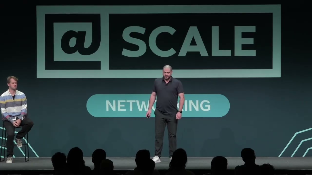
Live from SCCC: Physical Network Design at Scale | Brandon Premo and Richard Cziva — @Scale

@Scale

Transitioning from manual physical engineering to an automated design pipeline cuts Meta's data center network deployment timeline from months to days.

AI-assisted summary of Live from SCCC: Physical Network Design at Scale | Brandon Premo and Richard Cziva — original source. Check the original for full context.

Source published:

Detailed notes

## Background This presentation was published on YouTube by @Scale on August 31, 2026, featuring Meta engineers Brandon Premo and Richard Cziva live at the Santa Clara Convention Center. According to the page description, the session explores Meta's Loom system, an automated end-to-end pipeline designed to solve complex physical network design challenges driven by surging AI capacity demands.

## TL;DR To keep pace with the exponential growth of AI workloads, Meta transitioned from manual, 'artisanal' physical network design to an automated pipeline called Loom. The system orchestrates two primary components: Planogram, which uses lexicographic optimization and solvers to place devices across floorplans under strict failure domain constraints, and Fiber Design Automation, which materializes logical topologies into structured optical fiber networks. Already deployed across four production regions, Loom accelerates end-to-end network design from months to days while producing more reliable and standardized data center layouts.

## Atmosphere & style The presentation carries an authoritative, highly technical, yet reflective tone characteristic of a conference engineering talk. The speakers deliver a crisp and structured narrative, seamlessly balancing deep technical architectural details with pragmatic operational insights. As they reflect on organizational lessons—such as exposing ingrained habits masquerading as design rules—the talk builds an engaging emotional arc that transforms a dense infrastructure topic into a compelling story of engineering modernization.

## Key takeaways - [00:03](https://www.youtube.com/watch?v=0sebdRFvIc0&t=3s) Unprecedented AI workloads are forcing data centers to rapidly scale physical capacity and fiber infrastructure far beyond what manual design workflows can support. - [00:55](https://www.youtube.com/watch?v=0sebdRFvIc0&t=55s) To address the shortage of domain experts and eliminate slow, highly variable 'artisanal' manual design, Meta automated its end-to-end physical network design pipeline. - [03:00](https://www.youtube.com/watch?v=0sebdRFvIc0&t=180s) Logical topologies dictate connectivity rules and enforce non-proximate cabling across wide spaces, but traffic only flows after physical instantiation into racks and fiber. - [04:50](https://www.youtube.com/watch?v=0sebdRFvIc0&t=290s) Physical device placement creates a core tension: clustering devices simplifies fiber routing (fail-closed risk) while spreading devices maximizes fault tolerance (fail-open), but explodes cabling complexity. - [07:22](https://www.youtube.com/watch?v=0sebdRFvIc0&t=442s) Meta's Planogram engine uses lexicographic optimization to rank competing constraints—such as failure spreading, connectivity, and rack efficiency—without relying on arbitrary weighted scores. - [07:22](https://www.youtube.com/watch?v=0sebdRFvIc0&t=442s) Planogram resolves massive physical spatial complexity by combining graph decomposition, an Integer Linear Program (ILP) solver, and Reinforcement Learning (RL). - [11:09](https://www.youtube.com/watch?v=0sebdRFvIc0&t=669s) The Fiber Design Automation module materializes logical graph edges into physical optical paths using a structured cabling hierarchy (patch, breakout, trunk, and shuffle cables). - [14:03](https://www.youtube.com/watch?v=0sebdRFvIc0&t=843s) Channel schematics codify human engineering rules into reusable, location-agnostic patterns, enabling end-to-end software validation of polarity, cable compatibility, and path diversity prior to installation. - [14:03](https://www.youtube.com/watch?v=0sebdRFvIc0&t=843s) Automated fiber modeling generates precise early Bills of Materials (BOM) to mitigate supply chain lead times and produces step-by-step installation guides for field technicians. - [16:28](https://www.youtube.com/watch?v=0sebdRFvIc0&t=988s) The Loom pipeline is fully deployed across Meta production sites (4 regions, 20+ buildings), reducing device and fiber allocation time from months down to a few days. - [17:36](https://www.youtube.com/watch?v=0sebdRFvIc0&t=1056s) Frontloading power and spatial constraints catches physical infeasibilities early in software, eliminating costly re-work during physical data center deployment. - [18:18](https://www.youtube.com/watch?v=0sebdRFvIc0&t=1098s) A major organizational hurdle was translating informal human design intuition into precise mathematical objectives and unlearning deeply ingrained historical design habits. - [19:08](https://www.youtube.com/watch?v=0sebdRFvIc0&t=1148s) Future development focuses on expanding the automated framework to handle complex brownfield data center migrations and expansions.

## Detailed walkthrough ### [00:03](https://www.youtube.com/watch?v=0sebdRFvIc0&t=3s) The AI-Driven Shift in Data Center Capacity Demands

AI is fundamentally rewriting how data centers are designed and built by driving an unprecedented demand for capacity. This massive scale requires physical network designs to be created and delivered far faster than traditional processes were ever built to support. Higher capacity translates directly to a surge in network devices, which in turn demands significantly more supporting infrastructure like optical fiber for connectivity.

Compounding the sheer volume is operational complexity: capacity is no longer uniform. Instead, it arrives in diverse formats, including a hybrid mix of self-built data centers, leased facilities, and cloud infrastructure. Consequently, engineering teams must rapidly deploy vast amounts of capacity without the luxury of reusing a single static template across every project.

- AI workloads demand more data center capacity, faster delivery, and massive scaling of physical components like optical fiber. - Infrastructure deployment spans a heterogeneous mix: self-built data centers, leased sites, and cloud environments. - Traditional design workflows cannot keep pace with the needed speed or variations across different sites.

---

[00:55](https://www.youtube.com/watch?v=0sebdRFvIc0&t=55s) From Artisanal Design to End-to-End Automation

Historically, physical network infrastructure design was a manual, "artisanal" process. Each project was assigned a team of specialized engineers who had to meticulously study the unique physical properties of every data center building—including available power, failure domain boundaries, cooling constraints, and row/rack floorplan layouts. These experts manually solved the problem of mapping a logical network topology onto a given physical space and hand-crafted a corresponding fiber plan. This approach was inherently slow, introduced inconsistent design variations from engineer to engineer, and failed to scale alongside exponential AI growth.

To overcome the shortage of specialized experts relative to the overwhelming volume of projects, Meta transitioned to an end-to-end design automation pipeline. The automated system ingests the physical properties and constraints of a data center building or campus, selects the appropriate network topology for a project, maps that topology directly onto the unique physical floor plan, and generates a fully realized fiber connectivity design. Within this larger automation framework, two core modules drive the physical layout and cabling: **Planogram** and the **Fiber Design Automation** module.

- Manual physical design was slow, highly variable between individual engineers, and unscalable due to a shortage of domain experts. - The automated pipeline ingests site constraints, selects network topologies, maps devices to physical spaces, and outputs complete fiber plans. - Key presentation focus areas: Planogram (placement), Fiber Design Automation (cabling), and key operational lessons learned.

---

[03:00](https://www.youtube.com/watch?v=0sebdRFvIc0&t=180s) Bridging the Gap Between Logical Topologies and Physical Reality

For decades, networking research and engineering heavily prioritized logical topologies—focusing on switch layer stacking, interconnection rules, and traffic routing protocols. While logical topologies serve as critical blueprints, they do not carry a single bit of live traffic on their own. Actual network traffic runs over real fiber optic cables, inside physical racks, drawing power in physical rooms. Translating a logical blueprint containing thousands of devices into reality requires determining the exact row and rack for every single switch—a domain that historically received very little research compared to logical design.

``` +-----------------------------------------------------------------------+ | EXOSPINE (Aggregation Layer) | | +---------------+ +---------------+ +---------------+ | | | Plane 1 (XSW) | | Plane 2 (XSW) |... | Plane N (XSW) | | | +-------+-------+ +-------+-------+ +-------+-------+ | +-----------|-------------------|-----------------------|---------------+ | | | +-------------------+-----------------------+ | v +-----------------------------------------------------------------------+ | MEGAPOD BUILDINGS | | +-------------------+ +-------------------+ +---------------+ | | | Megapod 1 | | Megapod 2 | | Megapod M | | | | +-------------+ | | +-------------+ | | +----------+ | | | | | SSW1 | SSW2 | | | | SSW1 | SSW2 | | | |SSW1|SSW2| | | | | +-------------+ | | +-------------+ | | +----------+ | | | +-------------------+ +-------------------+ +---------------+ | +-----------------------------------------------------------------------+ ```

A prime example of a logical topology used at Meta features the "megapod" as a core building block—a set of leaf and spine switches (SSWs) configured in a Clos topology. Above the megapods sits an aggregation layer called the **exospine**, built from exospine switches (XSWs) organized into distinct "planes." In this architecture, a single plane connects exclusively to a specific spine index across every megapod in the entire region (e.g., Plane 1 connects to SSW1 in every megapod; Plane 2 connects to SSW2). This pattern introduces two major physical design implications: 1. Connectivity is dictated strictly by logical rules rather than physical proximity, forcing every plane to reach all corners of a building or region regardless of physical layout. 2. A plane represents a shared-fate region; losing a plane instantly cuts off that specific slice of the uplink across every single megapod simultaneously.

- Logical topologies provide essential blueprints but do not carry traffic without physical instantiation (racks, power, fiber). - The exospine aggregation layer uses planes of XSW devices connected to matching spine switch (SSW) indices in every megapod. - Exospine planes enforce non-proximate cabling requirements across wide physical spaces and create shared-fate failure dependencies.

---

[04:50](https://www.youtube.com/watch?v=0sebdRFvIc0&t=290s) The Fundamental Tension: Clustering vs. Spreading

Placing a logical topology onto a physical data center floor plan requires two simultaneous actions: grouping devices into physical racks and distributing those racks across distinct electrical failure domains. Connectivity must survive both steps—a plane must reliably reach its designated spine index in every megapod regardless of final rack locations. However, this process triggers a direct conflict between two opposing engineering instincts: grouping devices together for cabling simplicity versus spreading them apart for fault tolerance.

| Design Strategy | Fiber Footprint & Complexity | Failure Behavior / Blast Radius | Risk Classification | |:--- |:--- |:--- |:--- | | **Option 1: Clustering** <br> *(Group entire plane into one electrical failure domain)* | Minimal fiber required; simple routing (one trunk cable per plane). | **Maximal blast radius:** Losing one failure domain completely isolates a spine index across every megapod. | **Fail-closed** *(Unacceptable risk)* | | **Option 2: Spreading** <br> *(Scatter each plane across all failure domains)* | Fiber footprint explodes; every plane must reach all failure domains. | **Minimal blast radius:** Losing one failure domain results in a small, uniform ECMP bandwidth shrink across planes. | **Fail-open** *(Highly preferred)* |

- Physical placement forces a tradeoff between bundling devices together vs. distributing them across power domains. - Clustering minimizes fiber cabling but causes catastrophic fail-closed scenarios where entire planes go offline simultaneously. - Spreading mitigates failure impacts into soft ECMP capacity drops (fail-open), but dramatically increases cabling quantity and routing complexity.

---

[07:22](https://www.youtube.com/watch?v=0sebdRFvIc0&t=442s) Lexicographic Optimization and the Planogram Engine

Because engineering objectives conflict, Meta's engineers avoid blending tradeoffs into a single arbitrary, weighted mathematical score. Instead, they rank competing objectives in strict order of priority using **lexicographic optimization**. Under this approach, the optimization engine fully satisfies the top-priority objective before optimizing the second, ensuring lower-priority goals never compromise higher-priority constraints. The primary objectives include:

* **Connectivity Objective:** Minimizes the number of interconnecting rack pairs between adjacent layers, favoring physical grouping to create simpler, cheaper fiber designs. * **Failure Optimization Objective:** Spreads critical network entities across failure domains to keep outage impacts strictly within defined blast-radius budgets (counterbalancing connectivity). * **Row Similarity Objective:** Enforces uniform placement patterns across different rack rows to streamline site installation, maintenance, and operational field workflows. * **Rack Efficiency Objective:** Maximizes space and power utilization to pack required hardware into the smallest possible physical footprint.

Depending on site priorities, engineers reorder this ranked list; a cost-sensitive edge deployment might prioritize the connectivity objective at the top, while a resilience-critical flagship data center puts failure spreading first.

``` +-------------------------------------------------------+ | INPUT DATA | | 1. Logical Network Topology Graph (LNTG) | | 2. Physical Data Center Floorplan & Constraints | | 3. Ranked Optimization Objectives (Lexicographic) | +---------------------------+---------------------------+ | v +-------------------------------------------------------+ | PLANOGRAM ENGINE | | +-------------------------------------------------+ | | | Graph Decomposition Pass (Reduces Scale) | | | +------------------------+------------------------+ | | | | | v | | +-------------------------------------------------+ | | | Core Integer Linear Program (ILP) Solver | | | +------------------------+------------------------+ | | | | | v | | +-------------------------------------------------+ | | | Reinforcement Learning (RL) Module | | | | (Scales complex spaces & near-optimal variants) | | | +-------------------------------------------------+ | +---------------------------+---------------------------+ | v +-------------------------------------------------------+ | SOLVED OUTPUT | | Exact machine-readable map: Every device & rack | | pinned to a precise row, rack, and physical domain. | +-------------------------------------------------------+ ```

Simple greedy scripts fail at this task because physical constraints are deeply entangled, combinations scale exponentially, and competing priorities require principled tradeoffs. To solve this, Meta built **Planogram** (often referred to simply as **Plan**). At its core, Planogram utilizes an Integer Linear Program (ILP) solver. To prevent the massive scale of modern data centers from overwhelming the ILP, the system first executes a graph decomposition pass to break the problem into smaller, manageable sub-problems. Additionally, a Reinforcement Learning (RL) module explores near-optimal design variants and handles complex edge cases where strict ILP solvers struggle to scale. The resulting output is a machine-readable placement map that pins every switch to an exact row and rack position.

- Objectives are solved sequentially via lexicographic optimization without using arbitrary weighted scoring functions. - Planogram combines graph decomposition, an Integer Linear Program (ILP), and Reinforcement Learning (RL) to handle massive scale. - Output: A precise, machine-readable placement map that serves as the foundation for automated fiber cabling design.

---

[11:09](https://www.youtube.com/watch?v=0sebdRFvIc0&t=669s) Materializing Fiber Connections and Cable Plant Hierarchy

Once Planogram finishes mapping every device to a physical rack position, the **Fiber Design Automation** module generates the end-to-end fiber cable plant. The design starts with the Logical Network Topology Graph (LNTG), which defines every switch and logical edge in the network. Because Planogram has already pinned every node to a physical location, the fiber module's job is to "materialize" those logical edges into physical optical paths across the facility.

Running individual fiber patch cords directly between thousands of separated rack pairs is physically impossible due to massive cable volume and long distance constraints. To manage this density, the fiber automation system builds a structured hierarchy using specialized fiber cable products:

- **Patch Cords:** Single fiber-pair cables used for direct, short-distance connections. Simple, but unsuited for wide-area floorplan aggregation. - **Trunk Cables:** High-density, multi-fiber trunk lines that aggregate numerous connections onto shared high-capacity paths across rows and rooms. - **Breakout Cables:** Cables that group multiple individual device ports into a single high-density multi-fiber connector to feed directly into trunk cables, and unbundle them at the remote destination. - **Shuffle Cables:** Passive cable assemblies designed to cross-connect and redistribute individual optical fibers between connectors within the same cable bundle, enabling complex mesh topologies.

``` [ Device Interface A ] | (Single Fiber Pair) v [ Breakout Cable ] ---> Aggregates multiple connections onto a single connector | v [ Trunk Cable ] ------> High-density run across building rows / rooms | v [ Shuffle Cable ] ----> Passive internal optical re-mapping / cross-connect | v [ Breakout Cable ] ---> Splitting connections back to individual endpoints | v [ Device Interface B ] ```

In addition to physical aggregation, connections must satisfy strict fault-tolerance and path-diversity rules. High-availability layers require physical paths to be routed across totally disjoint physical infrastructure—meaning two redundant paths cannot share a common rack, patch panel, trunk enclosure, or cable tray.

- Logical edges from the LNTG are converted into physical fiber paths using Planogram's spatial placement data. - Structured cabling hierarchy leverages patch cords, breakout cables, high-density trunk cables, and shuffle cables. - Path diversity constraints require complete physical separation, ensuring alternative paths share zero single points of failure.

---

[14:03](https://www.youtube.com/watch?v=0sebdRFvIc0&t=843s) Channel Schematics and End-to-End Software Validation

To automate fiber design, Meta worked directly with veteran design engineers to extract and codify their manual design rules into standardized patterns called **Channel Schematics**. A channel schematic is a location-agnostic, abstracted representation of a fiber design pattern. It defines both the operational instruction set and the physical boundaries required to construct a valid fiber path regardless of a specific building's geometry.

``` +-------------------------------------------------------+ | CHANNEL SCHEMATIC RULES | | - Abstracted cabling patterns | | - Equipment constraints & cable product rules | | - Path diversity & redundancy requirements | +---------------------------+---------------------------+ | v +-------------------------------------------------------+ | BUILDING FLOOR PLAN | | - Physical rack locations (from Planogram) | | - Row layouts, rooms, and cable tray paths | +---------------------------+---------------------------+ | v +-------------------------------------------------------+ | FIBER AUTOMATION MODULE | | 1. Identifies optimal physical aggregation racks | | 2. Bundles fibers into shared trunk cable paths | | 3. Chains patch, breakout, trunk & shuffle cables | | 4. Validates polarity, connectors & continuity | +---------------------------+---------------------------+ | v +-------------------------------------------------------+ | DELIVERABLES | | - Complete software-validated fiber plant model | | - Accurate Bill of Materials (BOM) for procurement | | - Step-by-step rack installation guides for fields | +-------------------------------------------------------+ ```

Using these schematics, the automation engine analyzes a floor plan, selects optimal aggregation racks, bundles individual fiber links onto high-density trunk cables along shared physical paths, and chains the required cable products end-to-end. Because the resulting optical network is modeled as a complete software graph down to every individual strand, the system performs pre-construction software validation. It traces every link from its origin port in Rack A through all intermediate connectors and shuffle cables to its final destination in Rack B, automatically verifying hardware compatibility and correct optical polarity.

Capturing errors in software before physical deployment eliminates costly field re-work. The materialized fiber model serves as a single source of truth to automatically generate two critical operational outputs: an precise Bill of Materials (BOM) for early cable procurement (mitigating long supply chain lead times) and explicit, step-by-step rack installation instructions for field deployment technicians.

- Channel schematics codify manual design rules into re-usable, location-agnostic templates. - Complete software modeling allows automated end-to-end tracing to verify cable compatibility and optical polarity before installation. - Generates precise Bills of Materials (BOM) to accelerate long-lead procurement and produces step-by-step installation guides for field crews.

---

[16:28](https://www.youtube.com/watch?v=0sebdRFvIc0&t=988s) Real-World Scale, Velocity, and Impact

Addressing whether this pipeline is merely a research prototype or an active production system, Richard Cziva confirms that **every new data center Meta designs passes through this automated pipeline**. The system has already been deployed across four major regions, spanning more than 20 individual data center buildings and handling over 100 concurrent design variants.

``` +-------------------------------------------------------------------------+ | METRIC COMPARISON TABLE | +------------------------------+--------------------+---------------------+ | Process Stage | Manual Process | Loom Pipeline | +------------------------------+--------------------+---------------------+ | Initial Device & Fiber Alloc.| Months | A few days | | Design Revision/Reallocation | Weeks | Days | | Floorplan & Fiber Validation | Days | A couple of minutes | +------------------------------+--------------------+---------------------+ ```

Beyond sheer speed, automation delivers superior physical network designs compared to manual human engineering. By systematically eliminating human error, optimizing placement math, and strictly enforcing resilience constraints, the automated pipeline produces data center layouts that are demonstrably more reliable, efficient, and standardized.

- **Production Deployment:** In active use across 4 regions, 20+ data center buildings, and 100+ concurrent design variants. - **Speed Up:** Initial device and fiber allocation dropped from months to days; design re-allocations dropped from weeks to days; validation dropped from days to minutes. - Automated designs surpass manual efforts by maximizing physical reliability, eliminating human error, and optimizing spatial resource efficiency.

[17:36](https://www.youtube.com/watch?v=0sebdRFvIc0&t=1056s) Validation, Frontloaded Constraints, and Custom UI Visualization

Every generated design undergoes rigorous validation against network rules, during which the end-to-end fiber path is completely traced to ensure feasibility. By frontloading real-world power and space modeling directly into the automation pipeline, the system catches physical infeasibilities upfront. This eliminates the costly nightmare of discovering physical mismatches late in the process near the deployment phase. Furthermore, replacing the previous "designer-to-designer variable designs"—where every engineer introduced their own subtle variations and quirks—with automation ensures complete consistency across all network designs.

The presenters showcase a screenshot of a custom UI generated directly by one of their tools. This interactive interface allows network design engineers to visually inspect device placement across the floor plan, trace every individual fiber connection end-to-end, and manually perform modifications whenever necessary.

- Infeasibilities that previously surfaced late in deployment are now caught early through frontloaded power and space constraints. - Automation eliminates human variability between individual network designers. - The platform features a custom UI enabling visualization of device placement, fiber tracing, and manual adjustments.

[18:18](https://www.youtube.com/watch?v=0sebdRFvIc0&t=1098s) Organizational Lessons: Formalizing Objectives and Exposing Habits

Reflecting on the journey, the speakers share a slide that they wish their "younger self to see" before embarking on the project. When starting out, the team assumed the most formidable challenge would be the technical implementation—the automation, coding, and mathematical solvers. In reality, the true hurdle proved to be organizational.

The first major takeaway is that high-level objectives are far easier to state in plain English than to formalize into software logic. While a human expert can casually explain in five seconds to "spread things out for resilience," translating that loose concept into a precise, rankable objective function required months of effort. The second core lesson is how automation forces teams to confront rules that are actually just deeply ingrained habits. For instance, designers had routinely been leaving racks half-empty under the assumption it was necessary for future upgradability. When pressed for the underlying rationale, it turned out there was no real engineering reason—it was simply "tradition." Once objectives were made explicit, "these habits had nowhere left to hide."

- Objective formalization takes far more effort than technical coding or solver implementation. - Leaving half-empty racks for future upgrades was revealed to be a mere habit rather than a functional requirement. - Translating intuition like "spread things out for resilience" into mathematical cost functions required months of design work.

[19:08](https://www.youtube.com/watch?v=0sebdRFvIc0&t=1148s) Summary, Brownfield Expansion, and the Future of AI Network Design

To summarize their work, Meta created an automated physical network design pipeline where logical intent goes in and complete, physical network designs come out. The project remains under active development, with several next steps on the horizon. One of the most exciting future directions is brownfield design—adapting the same automation framework to function within already deployed, live production data centers to orchestrate complex network migrations.

This brings the discussion back to the core challenge: AI is rewriting how data centers are built faster than any manual engineering process can possibly maintain. Physical design can no longer be treated as an afterthought; it deserves to be automated, optimized, and studied as a "first-class problem." The session concludes with the speakers thanking the audience for their attention and opening the floor to questions.

- The system converts logical intent directly into physical network designs. - Next steps focus on brownfield data centers and automating complex network migrations in existing infrastructure. - Rapid growth driven by AI workloads mandates treating physical network design as an automated, optimized, first-class engineering problem.

## Notable quotes > [00:03](https://www.youtube.com/watch?v=0sebdRFvIc0&t=3s) AI is fundamentally rewriting how data centers are designed and built by driving an unprecedented demand for capacity. — Brandon Premo

> [00:55](https://www.youtube.com/watch?v=0sebdRFvIc0&t=55s) Historically, physical network infrastructure design was a manual, "artisanal" process. — Brandon Premo

> [03:00](https://www.youtube.com/watch?v=0sebdRFvIc0&t=180s) While logical topologies serve as critical blueprints, they do not carry a single bit of live traffic on their own. — Brandon Premo

> [03:00](https://www.youtube.com/watch?v=0sebdRFvIc0&t=180s) A plane represents a shared-fate region; losing a plane instantly cuts off that specific slice of the uplink across every single megapod simultaneously. — Brandon Premo

> [07:22](https://www.youtube.com/watch?v=0sebdRFvIc0&t=442s) Because engineering objectives conflict, Meta's engineers avoid blending tradeoffs into a single arbitrary, weighted mathematical score. — Brandon Premo

> [07:22](https://www.youtube.com/watch?v=0sebdRFvIc0&t=442s) Under this approach, the optimization engine fully satisfies the top-priority objective before optimizing the second, ensuring lower-priority goals never compromise higher-priority constraints. — Brandon Premo

> [11:09](https://www.youtube.com/watch?v=0sebdRFvIc0&t=669s) Running individual fiber patch cords directly between thousands of separated rack pairs is physically impossible due to massive cable volume and long distance constraints. — Brandon Premo

> [14:03](https://www.youtube.com/watch?v=0sebdRFvIc0&t=843s) Capturing errors in software before physical deployment eliminates costly field re-work. — Brandon Premo

> [16:28](https://www.youtube.com/watch?v=0sebdRFvIc0&t=988s) every new data center Meta designs passes through this automated pipeline. — Richard Cziva

> [18:18](https://www.youtube.com/watch?v=0sebdRFvIc0&t=1098s) The true hurdle proved to be organizational. — Richard Cziva

> [18:18](https://www.youtube.com/watch?v=0sebdRFvIc0&t=1098s) High-level objectives are far easier to state in plain English than to formalize into software logic. — Richard Cziva

> [18:18](https://www.youtube.com/watch?v=0sebdRFvIc0&t=1098s) these habits had nowhere left to hide. — Richard Cziva

> [19:08](https://www.youtube.com/watch?v=0sebdRFvIc0&t=1148s) Physical design can no longer be treated as an afterthought; it deserves to be automated, optimized, and studied as a "first-class problem." — Richard Cziva

## Mentioned Brandon Premo, Richard Cziva, Meta, Loom, Planogram, Plan, Fiber Design Automation, Logical Network Topology Graph, LNTG, Integer Linear Program, ILP, Reinforcement Learning, RL, Channel Schematics, Bill of Materials, BOM, Santa Clara Convention Center, SCCC, @Scale

[Source](https://www.youtube.com/watch?v=0sebdRFvIc0)

中文简报

Meta实现数据中心网络设计自动化以应对AI算力需求 从人工物理工程转向自动化设计流水线,Meta将数据中心网络部署周期从数月缩短至数天。 为跟上AI工作负载的指数级增长,Meta从人工“作坊式”物理网络设计转向了名为Loom的自动化流水线。该系统主要协调两大组件:Planogram利用字典序优化与求解器,在严格的故障域约束下将设备布置在机房平面图中;Fiber Design Automation(光纤设计自动化)则将逻辑拓扑落实为结构化光纤网络。Loom已在四个生产区域部署,将端到端网络设计周期从数月缩短至数天,同时生成了更可靠、更标准化的数据中心布局。 随着 AI 工作负载推动数据中心物理容量与光纤需求呈爆发式增长,传统耗时数月的手工“作坊式”网络设计流程已无法满足扩展需求。 (0:03) Meta 构建了端到端自动化物理网络设计系统 Loom,通过将逻辑拓扑直接映射到具体机房机架,将初始设计周期从数月缩短至几天,并已在 4 个区域、20 多栋数据中心建筑中投入生产。 (0:55) 设备布局引擎 Planogram 采用字典序优化(Lexicographic Optimization)协调故障扩散与布线复杂度之间的矛盾,结合图分解、整数线性规划(ILP)与强化学习(RL)实现精确的机架级设备放置。 (7:22) 光纤设计自动化模块借助通道原理图(Channel Schematics)将逻辑拓扑转化为端到端物理光纤路径,并在部署前通过全软件建模自动化校验光纤极性、连通性及物料清单(BOM)。 (14:03) 工程团队指出,项目最大的挑战在于将人类工程师模糊的经验直觉转化为严密的数学目标函数,并由此打破了传统设计中许多根深蒂固的无意义工程习惯。 (18:18)

Reading summary

To meet rapid capacity growth driven by AI workloads, Meta transitioned from manual data center physical network design to an automated pipeline that converts logical network topologies directly into optimized rack layouts and cabling plans. Automating the Bottlenecks of Artisanal Physical Design (0:03) AI infrastructure demands rapid delivery of network capacity across a heterogeneous footprint of self-built, leased, and cloud data centers. Historically, physical network design was an "artisanal" process where specialized engineering teams manually mapped logical topologies to specific building floorplans, cooling bounds, and power domains. This manual approach created inconsistent design variations between engineers and could not scale alongside exponential infrastructure demands. To resolve this shortage of specialized expertise, Meta implemented an end-to-end design automation system. The pipeline ingests campus physical constraints, selects appropriate network topologies, maps devices onto floorplans, and outputs fully realized fiber connectivity plans using two core components: the Planogram placement engine and the Fiber Design Automation module. Resolving Placement Conflicts with Lexicographic Optimization (4:50) Translating logical Clos architectures—such as Meta's megapod switch layers and exospine aggregation planes—onto physical racks introduces a conflict between cabling simplicity and fault tolerance. Clustering entire exospine planes into single electrical domains minimizes fiber cabling but creates an unacceptable fail-closed risk, where an outage isolates a spine index across every megapod. Conversely, spreading switches across failure domains establishes a resilient fail-open architecture via equal-cost multi-path (ECMP) capacity drops, but causes the physical fiber footprint to explode. Rather than relying on arbitrary weighted scoring, Meta's Planogram engine evaluates competing priorities sequentially using lexicographic optimization. The engine strictly satisfies higher-ranked objectives—such as failure domain blast-radius limits or inter-rack connectivity minimization—before evaluating secondary goals like row similarity and rack space efficiency. Planogram combines a graph decomposition pass, an Integer Linear Program (ILP) solver, and a Reinforcement Learning module to solve large-scale placements that overwhelm simple greedy algorithms. Materializing Optical Cabling through Channel Schematics (11:09) Once switches are placed, the Fiber Design Automation module converts abstract logical edges into physical cable plants. To eliminate the impracticality of running point-to-point patch cords between thousands of separated rack pairs, the system structures cabling into a hierarchy comprising patch cords, multi-fiber breakout cables, high-density trunk lines, and shuffle cables that passively redistribute fibers across connectors. The tool also enforces strict path diversity by ensuring redundant paths do not share racks, patch panels, enclosures, or cable trays. To automate this layout, Meta codified manual engineering rules into "Channel Schematics"—location-agnostic templates defining valid physical routing patterns. The system models the entire fiber plant as a software graph down to individual strands, enabling automated pre-construction validation of connector types, hardware compatibility, and optical polarity. This software model produces verified Bills of Materials to expedite supply chain procurement and yields step-by-step installation instructions for field technicians. Production Deployment Metrics and Organizational Takeaways (16:28) According to Richard Cziva, the automated pipeline is in active production across four regions, over 20 data center buildings, and handles more than 100 concurrent design variants. Compared to traditional manual methods, initial device and fiber allocation times dropped from months to days, design revisions fell from weeks to days, and validation was reduced from days to minutes. Early constraint modeling also catches physical power and space infeasibilities before construction begins, while a custom UI allows engineers to inspect placements and trace fiber paths. The engineering team found that organizational alignment posed a steeper challenge than solver development. Precisely formalizing intuitive concepts like "spreading for resilience" into mathematical objective functions required months of negotiation. Additionally, formalization exposed arbitrary legacy practices, such as leaving data center racks half-empty under the unverified assumption that it aided future upgrades. Meta plans to adapt this automation framework to brownfield environments to orchestrate complex network migrations within active data centers, arguing that the velocity of AI expansion requires physical network design to be treated as an automated, first-class engineering problem.

精炼阅读摘要

Brandon Premo 与 Richard Cziva 阐述了 AI 算力激增对数据中心交付速度和规模带来的颠覆性压力,指出传统人工设计物理网络已无法维系;为此 Meta 研发了一套端到端设计自动化流水线,将抽象的逻辑拓扑直接编译为经过数学优化、具备容错能力的物理机架布局与完整光纤布线方案。 逻辑映射的物理冲突与字典序求解 (4:50) 演讲者指出,逻辑网络拓扑(例如由 Clos 架构 megapod 构成的交换群与 exospine 汇聚层平面)不具备物理承载能力,必须具体映射到机房物理空间中。在映射过程中,工程上面临将设备聚合以简化布线,与将设备打散以分散供电故障域的根本冲突。若将属于同一平面的设备集中放置,光纤消耗最少但故障爆炸半径极大,单点供电故障就会切断所有 megapod 对应的上行链路(fail-closed);若将平面分散至所有故障域,虽然能借助等价多路径路由(ECMP)实现软性容量降级(fail-open),却会导致跨区域光纤布线量激增。为解决这一矛盾,Meta 摒弃了简单的人工加权评分算法,引入字典序优化(lexicographic optimization)机制,确保按严苛的优先级次序逐项满足目标。 负责物理布局的核心引擎 Planogram 会根据站点属性配置优先级队列,依次对连接性、故障分散、跨行一致性及机柜能耗空间利用率进行寻优。面对现代数据中心组合爆炸的庞大求解规模,Planogram 首先执行图分解预处理,将宏观拓扑拆解为子问题,随后调用整数线性规划(ILP)求解器进行核心计算,并辅以强化学习(RL)模块探索复杂边缘案例中的次优变体。该引擎最终输出机器可读的精确映射表,锁定每台交换机所在的具体物理行、机架及电气域,为后续自动化布线提供空间基准。 结构化布线抽象与端到端软件验证 (11:09) 当设备完成物理机架定位后,Fiber Design Automation 模块负责将逻辑拓扑图(LNTG)中的连边具象化为实际的光纤链路。鉴于海量分散机架之间不可能直接拉设单对跳线,系统建立了一套结构化布线层级:通过分支光缆(breakout)将单端口汇聚至高密度接头,经由主干光缆(trunk)实现跨房间或跨行的高密度传输,并利用洗牌光缆(shuffle)在光缆束内部完成被动交叉映射,最终再分解至对端设备。同时,系统在物理路径规划中严格执行路径多样性(path diversity)约束,确保互为冗余的链路在机柜、配线面板及线槽线路上实现完全物理隔离,杜绝单点失效。 为将原本依赖资深工程师的手工排线经验转化为算法逻辑,Meta 提炼出了与具体建筑空间解耦的“通道原理图”(Channel Schematics)。该模块基于原理图规则自动挑选最优聚合机架并进行光缆打捆,在软件层面构建出细致到每根单芯光纤的端到端数字模型。通过在施工前对光路全生命周期执行极性匹配、接口兼容性和连通性校验,流水线彻底消除了传统现场施工中的返工成本,并能自动导出精准的物料清单(BOM)以应对漫长采购周期,同时生成指导现场作业人员的分步机架安装说明。 生产部署规模与端到端交付提速 (16:28) Richard Cziva 证实,该自动化流水线并非实验室原型,而是已全面承载 Meta 每一个新建数据中心的设计交付。系统已在 4 个主要大区上线运行,覆盖 20 余栋数据中心建筑,并支持超过 100 个并发设计变体的并行迭代。在交付效率方面,端到端自动化取得了数量级的跨越:最初的设备与光纤分配周期由以往的数月压缩至数天,面对需求变更的设计重排由数周缩短为数天,而建筑平面与光纤路径的合规校验则从以往的数天降至数分钟以内。 除了显著提升工程流转速度,自动化生成在质量维度同样超越了传统手工设计。流水线将供电规格与物理空间约束前置到设计初期,在架构阶段即识别出物理不可行性,规避了临近部署阶段才发现空间或电力错配的风险。此外,标准化规则彻底消除了以往不同设计师之间因个人风格而产生的琐碎差异。配合专门研发的定制可视化交互界面,工程团队能够直观审视机架布局、追踪端到端单芯光纤走向并执行必要微调,使布局方案在物理可靠性与标准化程度层面达到最优状态。 组织认知重塑与工程陈规破除 (18:18) 演讲者在总结复盘时指出,该系统构建过程中最大的工程阻力并非算法设计或数学求解器实现,而是组织层面的概念形式化与认知转变。在实践中,人类专家能用日常语言在数秒内提出的高层直觉(例如“为了弹性尽量将设备打散”),但在将其转化为软件能够执行、优先级分明的精确数学目标函数时,团队耗费了数月时间反复推敲与建模。 与此同时,自动化推行过程迫使工程团队正面审视并清除了大量被伪装成技术规范的组织陈规。例如,过去现场工程师在设计机架时普遍习惯性保留半空机位,并声称这是为了满足未来的升级扩容需求;但当系统要求提供底层的量化工程论据时,团队发现该做法并无实质技术支撑,仅仅是一项长期沿袭的传统习惯。通过将工程意图全部显式转化为可审查的代码逻辑,系统使此类缺乏论证的工程惯性无处遁形,推动了数据中心架构定义的制度化规范。 Meta 目前正在将这套自动化物理网络设计流水线从新建项目推广至存量(brownfield)数据中心,以支持在线生产环境下的复杂网络平滑迁移。演讲者强调,AI 驱动的超大规模基础设施建设使得物理层面的物理机架摆放与光纤敷设不再是逻辑设计的从属附件,而必须被视作需要深度建模、数学优化与全自动化处理的核心工程课题。

Detailed notes — zh

## Background 本视频由 YouTube 频道 @Scale 于 2026 年 9 月 3 日发布,记录了来自 Meta 的 Brandon Premo 与 Richard Cziva 在圣克拉拉会议中心(SCCC)的现场技术演讲。内容聚焦于应对 AI 浪潮下爆发的数据中心网络容量需求,介绍了 Meta 研发的物理网络自动化设计系统 Loom,该系统通过协同设备摆放引擎(Planogram)与光纤设计模块,将传统长达数月的物理网络设计流程压缩至数小时。 ## TL;DR 面对 AI 时代极速扩张的数据中心容量与多元机房形态,传统依赖人工专家经验的物理网络设计面临扩展极限与标准不一的困境。为此,Meta 构建了端到端物理网络自动化设计管道 Loom,其设备布局引擎 Planogram 采用整数线性规划(ILP)、图分解与强化学习,通过严格的词典序多目标优化破解了布线成本与容灾故障域打散之间的核心冲突。在此基础上,光纤设计模块基于脱离具体坐标的“通道示意图”规范,将逻辑拓扑自动化具象化为高密度主干与分支光纤物理连接,并实现了端到端极性软件仿真校验与物料清单自动导出。该系统已在 Meta 生产环境全面投产落地并覆盖数十栋建筑,同时倒逼工程团队破除未经验证的传统设计陋习,实现了从经验主义到形式化数学建模的组织范式跃迁。 ## Atmosphere & style 整场演讲展现出顶级科技大厂基础设施团队兼具严谨数学美感与硬核工程落地的工业沉淀风格。两位主讲人配合默契、逻辑推进层层剥茧,既有在白板层面化解组合爆炸与运筹优化的理性冷静,又有深谙现场拉线、空间电力过载等现实泥潭的生动工程洞察。演讲尾声关于“自动化倒逼团队识别伪装成经验的习惯”的真诚复盘格外令人触动,让观众深刻体会到系统从“手工作坊”跨越至“数学驱动自动化”过程中带来的工程震撼与思维蜕变。 ## Bulletin - [01:54](https://www.youtube.com/watch?v=0sebdRFvIc0&t=114s) Meta 构建了端到端物理网络自动化设计系统 Loom,将原本需要耗时数月的手工数据中心布局与光纤设计压缩至数天甚至数小时内完成。 - [09:59](https://www.youtube.com/watch?v=0sebdRFvIc0&t=599s) 系统核心包含 Planogram 放置引擎与光纤自动化设计模块,分别基于整数线性规划(ILP)求解设备机架排布,以及基于通道示意图(Channel Schematic)生成端到端物理光纤布线。 - [07:22](https://www.youtube.com/watch?v=0sebdRFvIc0&t=442s) Planogram 采用词典序多目标优化而非加权打分,严格按照业务优先级依次满足连接成本、故障隔离域、行相似度与机架空间利用率等相互冲突的目标。 - [16:28](https://www.youtube.com/watch?v=0sebdRFvIc0&t=988s) Loom 已全面投入生产,应用于 4 个大区、20 余栋建筑并并发支持 100 多种设计变体,端到端光路验证时间从数天大幅缩短至数分钟。 ## Key takeaways - [00:03](https://www.youtube.com/watch?v=0sebdRFvIc0&t=3s) AI 工作负载驱动数据中心容量需求爆发,涵盖自建、租赁与云设施等多元形态,传统依赖专家人工经验的物理网络设计已无法横向扩展。 - [02:48](https://www.youtube.com/watch?v=0sebdRFvIc0&t=168s) 逻辑拓扑(如 Megapod 与 Exospine)本质上是不承载流量的蓝图,真实流量必须在机房内消耗电力和机架空间的物理光纤上流淌。 - [04:50](https://www.youtube.com/watch?v=0sebdRFvIc0&t=290s) Exospine 平面连接基于逻辑属性而非物理邻近,导致物理设计面临“物理聚集以降低光纤成本”与“彻底打散以隔离故障域”的本质冲突。 - [04:50](https://www.youtube.com/watch?v=0sebdRFvIc0&t=290s) 将平面设备集中放置会导致单点断电引发平面瘫痪的闭合性失效(Closed failure);而彻底打散虽然增加布线,但能确保断电时仅触发优雅的 ECMP 收缩降级。 - [07:22](https://www.youtube.com/watch?v=0sebdRFvIc0&t=442s) 传统贪心脚本因约束高度纠缠和组合爆炸在大规模场景下失效,Loom 采用词典序多目标优化(Lexicographic optimization)数学引擎求取可证明的最优解。 - [09:59](https://www.youtube.com/watch?v=0sebdRFvIc0&t=599s) 为防止 ILP 求解器在超大规模数据中心计算爆炸,Planogram 结合了图分解技术与强化学习(RL)探索机制以处理极限解空间。 - [12:24](https://www.youtube.com/watch?v=0sebdRFvIc0&t=744s) 在大规模园区中点对点跳线在物理上不可行,必须依托主干光缆(Trunk)、分支光缆(Breakout)与洗牌光缆(Shuffle Cable)构建结构化光纤网络。 - [12:24](https://www.youtube.com/watch?v=0sebdRFvIc0&t=744s) 容灾网络要求满足严格的物理路径多样性(Path Diversity),互为冗余的链路严禁共享相同的机架、线缆和走线管道路径。 - [14:03](https://www.youtube.com/watch?v=0sebdRFvIc0&t=843s) 通过定义位置无关的“通道示意图”(Channel Schematic),系统将专家布线规则形式化,实现软件端到端光路回溯、接头匹配与极性方案校验。 - [14:03](https://www.youtube.com/watch?v=0sebdRFvIc0&t=843s) 数字化的端到端光纤模型使物料清单(BOM)能够提前自动生成以应对供应链超长交付周期,并自动输出施工现场逐机架安装指南。 - [16:28](https://www.youtube.com/watch?v=0sebdRFvIc0&t=988s) Loom 在生产环境中全面落地,在提升效率的同时将电力和空间约束前置,消除了由于人工主观习惯产生的设计缺陷与不一致性。 - [18:18](https://www.youtube.com/watch?v=0sebdRFvIc0&t=1098s) 项目落地的最大阻力在于组织协同与模糊工程经验的数学形式化,自动化过程迫使团队审查并剔除了诸如“机架无理由空置一半”等缺乏科学依据的传统陈规。 - [18:18](https://www.youtube.com/watch?v=0sebdRFvIc0&t=1098s) Loom 下一步的技术路线重点是存量(Brownfield)数据中心建模,旨在利用同一套自动化管线协同完成带电生产环境中的复杂在线架构割接与迁移。 ## Detailed walkthrough ### [00:03](https://www.youtube.com/watch?v=0sebdRFvIc0&t=3s) AI 浪潮下的数据中心容量挑战与传统物理网络设计的瓶颈 人工智能(AI)正在彻底重构数据中心的建设方式。AI 工作负载引发了前所未有的数据中心容量需求,这种海量容量必须以前所未有的速度完成设计和交付,其紧迫性与规模远超现有交付流程的设计承载能力。更多的网络容量意味着指数级增长的网络设备,以及连接这些设备所需的数以百万计的光纤等物理组件。更棘手的是,这些容量并不是单一形态的,而是由自建数据中心(Self-built)、租赁机房(Lease sites)以及公有云基础设施(Cloud infrastructure)等多元形态混合而成。面对高复杂性与高交付速度的双重夹击,团队显然无法在不同的项目中简单套用相同的模板。 在此之前,物理网络基础设施的设计主要是一种“手工作坊式”(Manual artisanal process)的流程。每个项目都会指派一组专门的设计师与领域专家,他们必须深入了解每栋数据中心建筑的具体物理属性,包括可用电力、故障域(Failure domain)设计、冷却条件以及机架排(Row/Rack)的物理布局。工程师需要纯靠人工推演,将上层的网络拓扑映射到特定的物理空间中,并为每个项目定制生成详细的光纤连接设计方案。 这种人工主导的流程极其缓慢,不仅在不同工程师之间会产生不可控的设计差异(Design variance),而且根本无法随业务规模横向扩展。随着数据中心容量需求的持续井喷,项目数量远远超出了现有专家团队的人力负荷,推动设计范式向自动化变革已迫在眉睫。 - 容量形态多元化:涵盖自建数据中心、租赁机房与云基础设施,无法简单复用单一蓝图。 - 传统人工设计的弊端:高度依赖专家经验、设计周期长达数月、工程师之间存在主观差异、无法支撑 AI 时代的超大规模扩张。 --- ### [01:54](https://www.youtube.com/watch?v=0sebdRFvIc0&t=114s) 端到端物理网络自动化设计管道:Loom 系统的诞生 为了打破产能瓶颈,Meta 转向了全流程自动化,将原本交织混乱的设计流程拆解为独立的标准化环节,构建了一套端到端的物理网络设计自动化管道(即 Loom 系统)。该系统能够原生理解数据中心建筑及整个园区的物理属性与工程约束,自动评估并选择与特定项目最匹配的网络拓扑架构,将抽象的拓扑结构精准映射至各异的物理机房空间,并最终自动化输出连接所有网络实体的端到端光纤连接方案。 在这套自动化体系中,核心由两大关键组件驱动:首先是由 Richard Cziva 介绍的设备摆放与布局引擎——**Planogram**,它负责在满足物理空间和故障域约束的前提下完成网络设备机架的安放;其次是由 Brandon Premo 介绍的光纤设计自动化模块(Fiber Design),负责生成满足复杂物理约束的光纤布线方案。整套系统将以往长达数月的端到端物理网络设计周期压缩至几小时以内。 ```mermaid flowchart TD accTitle: 端到端物理网络设计自动化流程 accDescr: 展示从物理空间与拓扑输入到 Planogram 设备放置再到光纤连接生成的完整自动化链路 subgraph Inputs["输入规格与约束"] A["物理建筑与园区约束<br/>(电力/空间/冷却/机柜布局)"] B["逻辑拓扑规格<br/>(Megapod/Clos 拓扑)"] C["多目标工程优先级<br/>(词典序优化目标)"] end subgraph Pipeline["Loom 自动化设计管道"] D["拓扑选型与物理映射"] E["Planogram 放置引擎<br/>(机架编排与故障域分配)"] F["光纤设计模块<br/>(端到端物理连接生成)"] end subgraph Outputs["最终交付成果"] G["设备机架放置图纸<br/>(Rack-level Layout)"] H["光纤连接方案与布线表<br/>(Fiber Connectivity)"] end A --> D B --> D C --> E D --> E E --> F E --> G F --> H ``` --- ### [02:48](https://www.youtube.com/watch?v=0sebdRFvIc0&t=168s) 逻辑拓扑与物理现实的脱节:从 Megapod 到 Exospine 架构 在深入探讨设备摆放问题之前,必须正视学术界与工业界长期存在的视角盲区:几十年来,整个网络领域投入了海量精力研究逻辑拓扑(Logical topology)——探讨网络层级如何堆叠、交换机之间如何互联以及流量如何在不同路径之间路由。这些研究固然深刻且不可或缺,每一个网络设计也确实始于逻辑拓扑,但正如演讲中所强调指出的:“逻辑拓扑不承载任何一个比特的实际流量,它本质上只是一张蓝图。流量最终是在实体机房内消耗电力、安放在物理机架中的光纤上流淌的。”("A logical topology doesn't serve a single bit of traffic. It really is just a blueprint. Traffic runs on fiber in racks drawing power in a real room.")必须有人将这张蓝图落地,为成千上万台交换设备决定其具体的排位(Row)与机架位(Rack)。这一关键的落地环节长期以来几乎完全依靠人工和专家经验,不仅缓慢,而且在不同工程师乃至不同大区(Region)之间充斥着不一致性。 以 Meta 长期大规模使用的典型网络拓扑为例:网络的基础构建单元是 **Megapod**,它是由 Leaf 和 Spine 交换机(SSW)构成的标准 Clos 拓扑;位于 Megapod 之上的是汇聚层,被称为 **Exospine**。Exospine 由大量的 XSW 设备组成,并划分为不同的平面(Planes)。其连接模式呈现出严格的规则:每一个平面(Plane)只连接整个大区内所有 Megapod 中相同索引位置的 Spine 交换机。例如,Plane 1 连接所有 Megapod 的 SSW 1,Plane 2 连接所有 SSW 2,以此类推。 这种逻辑拓扑结构带来了两个极为严苛的物理工程后果: 1. **连接基于逻辑属性而非物理邻近性(Connectivity is by logical property, not by proximity)**:无论 Megapod 在建筑物或园区内的物理位置相隔多远,每一个平面都必须将光纤物理延伸到机房和大区的每一个角落。 2. **平面即共享故障域(Shared fate)**:一个平面就是一个大区级别的共享失效域。一旦失去某一个平面,大区内的每一个 Megapod 都会在同一时刻失去其对应索引的上行链路带宽分片。 --- ### [04:50](https://www.youtube.com/watch?v=0sebdRFvIc0&t=290s) 物理落地的核心冲突:聚集(Clustering)与打散(Spreading)的权衡 将抽象的 Exospine 逻辑拓扑映射到机房物理平面图(Floor plan)包含两个紧密交织且必须同步求解的动作:第一步是将逻辑交换设备归入机架(Racking),例如将 SSW 按 Megapod 装柜,将 XSW 按平面装柜;第二步是将装好设备的机架放置在机房的不同区域,本质上是将它们分配到不同的**电气故障域(Electrical failure domains)**中。无论机架被移动到物理平面的何处,前述“每个平面直连特定索引 SSW”的逻辑连接约束都必须严格得到满足。正是在这种将设备“汇聚入机架”与在物理平面上“横向分散打散”的双重本能拉扯下,物理设计面临剧烈的工程冲突。 这一冲突集中体现在如何将 Exospine 交换机安置在各个电气故障域中: - **方案一:集中放置(Clustering)** 将整个平面的设备全部放置在同一个电气故障域内(例如将 Plane 1 完全放入电气故障域 1)。这种方案的优势在于物理连线极少,每个平面仅需一条聚合主干光缆(Trunk)即可引出,布线极其简单经济。然而,一旦模拟该电气故障域整体断电失效,灾难便会降临:整个 Plane 1 全军覆没,大区内所有 Megapod 对应的同一组 Spine 上行链路瞬间全部中断。这种失效被称为“闭合性失效”(Closed failure),造成了最大化的爆炸半径(Blast radius),在工程生产中是绝对无法容忍的。 - **方案二:彻底打散(Spreading)** 将每一个平面的设备打散分布到所有的电气故障域中(Plane 1 的设备被均匀散布在各个故障域)。此时,光纤开销呈现爆炸式增长,每一个平面都必须拉线通往机房的每一处区域。但当某个电气故障域遭遇断电完全瘫痪时,没有任何一个 Megapod 或平面会被完全孤立,各个平面仅仅损失了一小部分等价多路径路由(ECMP)容量。这种失效被称为“开放性失效/ECMP 收缩”(Open failure / ECMP shrink),是高弹性网络架构首选的优雅降级模式。 这两种方案展现了完全相同的逻辑拓扑在不同物理分配策略下带来的截然相反的系统特性。Planogram 的核心使命,正是要将这种在光纤布线成本与系统容灾韧性之间的矛盾显式化、量化排序并求出最优解。 | 布局策略 | 放置方式 | 光纤与布线成本 | 电气故障域失效后果 | 故障模式与爆炸半径 | |:--- |:--- |:--- |:--- |:--- | | **集中放置 (Clustering)** | 单个平面所有设备集中于单一故障域 | 极低(每个平面仅需极少光纤主干,走线简单) | 整个平面完全瘫痪,所有 Megapod 对应索引链路全断 | 闭合性失效(Closed failure),爆炸半径最大化(不可接受) | | **打散放置 (Spreading)** | 单个平面的设备均匀分散至所有故障域 | 极高(光纤数量爆炸,每平面需跨区域全面互联) | 各平面仅损失一小截容量,无节点孤立,触发 ECMP 收缩 | 开放性失效(Open failure),爆炸半径可控(高度推荐) | --- ### [07:22](https://www.youtube.com/watch?v=0sebdRFvIc0&t=442s) 词典序多目标优化:破解贪心脚本与启发式算法的死局 当工程师配置这些相互冲突的工程诉求时,他们绝不会提供一个简单的综合得分权重,而是给出一个严格排列优先级的**目标优先级清单(Ranked list)**。Planogram 系统将这些工程诉求提炼为四大约束目标: 1. **连接优化目标(Connectivity objective)**:尽可能减少相邻网络层级之间互联的机架对数量,从而生成更简单、造价更低的光纤物理连接(偏向物理聚集本能)。 2. **故障容灾目标(Failure optimization)**:将相关网络实体最大限度分散到不同的故障域中,严格控制在故障预算(Blast radius budget)之内(偏向物理打散本能)。 3. **行相似度目标(Row similarity objective)**:在不同机架排之间实现高度统一标准化的设备排列,极大降低现场施工部署与后期运维的认知与操作复杂度。 4. **机架空间效率目标(Rack efficiency objective)**:以最紧凑的物理空间与电力开销容纳给定规模的网络设备。 针对这些相互竞争的目标,系统绝不采用“加权评分魔法系数函数”(Weighted score magic coefficient function)进行模糊折中,而是采用严格的**词典序多目标优化(Lexicographic optimization)**:引擎首先必须百分之百完全满足排名第一的高优先级目标;在此前提下,继续优化第二目标,且在此过程中绝对不允许损害第一目标已达成的优化结果。目标优先级的排列完全取决于业务场景的选择——对于成本敏感型(Cost-sensitive)部署,可将连接优化放在最前;而对于业务可用性极度敏感(Resilience-critical)的场景,则将故障打散放在首位。底层使用相同的数学引擎,无论哪种取舍都能输出在数学上可证明的最优方案。 许多网络工程师初次面对设备摆放问题时,本能反应往往是“这不就是三维装箱问题(Bin packing)吗?写一个贪心脚本(Greedy script)跑一下就行了”。但在超大规模现实场景下,贪心脚本必然失效,其原因有三: - **约束高度纠缠(Tangled constraints)**:现实物理与电气规则盘根错节,脚本修复了一个约束,往往直接破坏了另一个约束。 - **超大规模组合爆炸(Combinatorial explosion)**:面对数千个网络实体、复杂的网络拓扑以及多变的空间布局,其排列组合空间远远超出了任何简单启发式算法的有效处理范围。 - **目标本质互斥(Fighting objectives)**:低成本光纤与高容灾生存能力对立,紧凑装箱与标准化排布对立。硬编码的贪心脚本只能强行指定胜者,而无法在全球最优的框架下动态求得平衡。 --- ### [09:59](https://www.youtube.com/watch?v=0sebdRFvIc0&t=599s) Planogram 系统架构:从整数线性规划(ILP)到图分解与强化学习 为了在数学上可证明有效的前提下高效求解这个庞大的布局难题,Meta 构建了 Planogram 系统。从系统外部看,它统一接收三项核心输入: - 上层网络架构的**逻辑拓扑(Logical topology)**; - 现场建筑机房的**平面图与工程约束(Floor plan)**; - 工程师定义的**词典序多目标优先级列表(Objectives)**。 而在系统内部,承担核心计算重任的是一套底层的**整数线性规划(Integer Linear Programming, ILP)**引擎。ILP 能够直接建模极其复杂的物理约束与设备摆放规则,输出可证明的全局最优布局方案。 然而,在成千上万台设备的超大数据中心场景下,如果直接将全局参数抛给 ILP 求解器,求解器会因计算状态空间过大而彻底“窒息”(Choke)崩溃。为了突破算力天花板,Planogram 架构引入了混合求解机制:首先通过图遍历与图分解阶段(Graph pass),将庞大的拓扑与机房物理结构解耦为若干独立受控的较小子问题,显著降低数学复杂度;同时,系统集成了一个**强化学习(Reinforcement Learning, RL)模块**,在纯数学 ILP 求解器难以扩展的超大规模边界下接管搜索过程,能够在极短时间内探索并输出一整族接近全局最优(Near-optimal variants)的高质量可行解,赋予工程团队更灵活的设计决策空间。 - **系统核心输入**:逻辑拓扑、物理平面图、排序后的工程优化目标。 - **底层计算核心**:整数线性规划(ILP),确保解的严格最优性。 - **可扩展性支撑**:采用图算法分解(Graph decomposition)化简维度,结合强化学习(RL)在大规模极限场景下高效探索近似最优解空间。 ### [10:48](https://www.youtube.com/watch?v=0sebdRFvIc0&t=648s) 从放置到光纤:将逻辑拓扑具象化为物理连接 在 Planogram 完成设备排布计算后,整个数据中心平面图的求解便告完成。拓扑结构中的每一个网络设备和机架都在机房地面上找到了具体的物理坐标,形成了一张精确的、机器可读的设备位置图。这正是后续光纤自动化设计的基础。接下来的核心任务,就是将这张图转化为实际的光纤布线方案。 设计光纤连接所依据的依然是逻辑网络拓扑图(LNTG, Logical Network Topology Graph)。LNTG 作为高层逻辑设计,详尽定义了网络中的每台设备以及它们之间的所有互联关系。既然 Planogram 已经确定了每个节点的物理位置,现在的目标就是将 LNTG 中的每一条逻辑边(Logical Edge)具象化为现实中可铺设的物理光纤链路。需要连接的设备往往分散在整个园区的不同区域:有些是同排相邻的机架,有些需要跨排互连,有些要穿过不同的机房房间,甚至需要跨越不同的建筑物。随着网络规模的扩大,连接需求迅速累积,如果简单地在每一对机架之间直接拉线,布线空间会瞬间被塞满;由于距离过长且线缆数量极其庞大,点对点直连在物理工程上根本不可行,必须引入结构化的线缆组织方式。 ```mermaid flowchart TD accTitle: Logical to Physical Fiber Mapping accDescr: Pipeline transforming the Logical Network Topology Graph into physical fiber connections using Planogram rack placements. subgraph Logical["逻辑层 (LNTG)"] L1["设备 A"] ---|"逻辑链路 (Logical Edge)"| L2["设备 B"] end subgraph Placement["物理定位 (Planogram)"] P1["机架 A 定位<br>(行/列/房间)"] P2["机架 B 定位<br>(行/列/房间)"] end subgraph Physical["物理光纤布线层"] F1["端口连接"] --> F2["分路汇聚 (Breakout)"] F2 --> F3["主干光缆 (Trunk Cable)"] F3 --> F4["解复用/分支"] F4 --> F5["对端端口"] end Logical --> Placement Placement --> Physical ``` - **逻辑网络拓扑图(LNTG)**:包含所有网络设备与互联关系的逻辑蓝图,为物理布线提供驱动依据。 - **直连弊端**:跨排、跨房间、跨楼宇如果全采用点对点跳线,线缆数量与布线距离会导致线槽空间迅速耗尽且不可维护。 --- ### [12:24](https://www.youtube.com/watch?v=0sebdRFvIc0&t=744s) 光缆产品谱系与路径多样性约束 为了解决大规模线缆聚合的问题,物理光纤基础设施采用了多种针对性线缆类型。最基础的是常规跳线(Patch Cord),即单对光纤直连,简单但缺乏扩展性与灵活性。在实际工程中,系统采用高密度连接器的主干光缆(Trunk Cable)实现链路汇聚,将大量连接收拢至单根主干缆中长途传输。前端通过分支光缆(Breakout Cable)将分散的单路连接打包装入单颗高密度接头并接入主干缆;到达远端机架后,再通过另一根 Breakout Cable 将多路信号重新分拆回独立的单对接口。此外,系统还引入了洗牌线缆(Shuffle Cable),用于在同一根线缆的各个连接器之间重新分配和交叉映射纤芯,满足特定网络架构严苛的纤芯映射需求。 然而,线缆设计并不仅仅是把两端连通,每一层互联网络都伴随着严格的容错与冗余要求。为了保障高可用性,同一逻辑层的多条链路必须强制分散在多条完全独立的物理路径上,即满足路径多样性(Path Diversity)。一条真正的独立路径必须具备物理隔离性——不能共享相同的机架、不能共用同一根线缆,并且必须在建筑内走行完全不同的路由管道。唯有如此,当某条路径遭遇物理损坏或执行日常维护停机时,其余互补链路才能维持数据中心的持续运转。 - **跳线(Patch Cord)**:单纤对直连线缆,用于短距与简单接入,无法应对高密度聚合。 - **主干光缆(Trunk Cable)**:采用高密度接头,单根线缆聚合传输多对光纤。 - **分支光缆(Breakout Cable)**:在汇聚点将多路离散物理连接归并到高密度接头,或在远端反向分拆。 - **洗牌线缆(Shuffle Cable)**:在内部跨接头重排纤芯走向,实现特殊的拓扑矩阵映射。 - **物理路径多样性标准**:容灾链路之间严禁共用任何物理组件(包含机架、走线桥架与物理线缆),且走向必须物理分离。 --- ### [14:03](https://www.youtube.com/watch?v=0sebdRFvIc0&t=843s) 通道示意图与端到端光纤建模校验 为了把资深工程师脑中的布线经验转化为计算机可执行的算法,工程团队与设计专家深度协作,将原本手工设计中常用的布线套路与物理容灾规则提炼并代码化,形成了所谓的“通道示意图”(Channel Schematic)。Channel Schematic 是一种脱离具体物理机房坐标的位置无关(Location-Agnostic)抽象模式,它既是指导自动化引擎串接线缆的操作指令集,也是布线算法必须满足的硬性约束。利用这套设计规则,系统可以将其无差别地套用在任何平面布局的数据中心项目上。 在实际执行中,系统结合 LNTG 链路需求与数据中心物理空间结构,自动识别哪些机架适合作为线缆汇聚点,将共享相同路由与终点的纤芯打包进主干光缆,并按照 Channel Schematic 的结构规范级联各类光缆部件,建立从起始设备物理接口直至远端对等体物理接口的端到端(End-to-End)链路。整套光纤网络全面完成数字化建模后,软件便能对所有线缆与连接器进行端到端的全量虚拟追踪。校验引擎能跟踪从机架 A 端口出发、穿过所有跳线与主干链路、最终接入机架 B 端口的完整光路,提前核验所有接头型号匹配度以及全链路的极性规划(Polarity Plan)。这种在设计阶段即完成的软件仿真,把过去往往要在机房现场施工安装时才会暴露的极性颠倒或接口不匹配问题消灭在了萌芽状态。 ```mermaid flowchart LR accTitle: Fiber Validation and Production Workflow accDescr: End-to-end process from automated path validation to material generation and field instructions. subgraph Validation["端到端软件校验"] direction TB V1["光路追踪<br>(机架 A 到机架 B)"] --> V2["接头/线缆兼容性"] V2 --> V3["极性方案校验 (Polarity)"] end subgraph Downstream["下游工程交付"] direction TB D1["物料清单 (BOM) 自动生成<br>提前采购应对超长货期"] D2["逐机架施工安装手册<br>(Field Instructions)"] end Validation ==>|"校验通过的纤芯模型"| Downstream ``` - **通道示意图(Channel Schematic)**:对光纤连接架构进行抽象建模的位置无关规则规范,定义了自动化线缆级联的指令与约束边界。 - **端到端极性与兼容性校验**:通过软件回溯光纤端到端完整物理链路,提前排查极性反转与物理规格不匹配缺陷。 - **下游交付提速**:数字化光纤模型可直接自动导出精准的线缆物料清单(BOM),大幅提前采购下料以对冲供应链长交付周期(Lead Times),同时自动生成面向现场施工人员的逐机架安装指南。 --- ### [16:28](https://www.youtube.com/watch?v=0sebdRFvIc0&t=988s) 生产落地成果:规模、性能与设计质量跃迁 针对外界对该系统是否仅为“实验室原型”的疑虑,Richard Cziva 明确表示,Loom 已经全面进入生产运营,目前 Meta 设计的每一座新数据中心都必须经过该自动化管线。该系统已在 4 个大区、超过 20 栋建筑中正式投用,并同时处理过 100 多种并发设计变体(Concurrent Design Variants)。自动化带来的效率提升是数量级的:原本需要耗费数月的设备排布与光纤分配工作,现在缩短到了短短几天;过去因工程变更需要花费数周进行重新调整的工作,现在同样只需几天即可重新收敛;而在验证环节,针对设备空间与光缆连通性的全量校验,从原先的数天直接压缩至数分钟之内。 更为关键的是设计质量的跃升。Cziva 强调,“快速做出的糟糕设计依然是糟糕设计”,而 Loom 生成的方案在三个维度上显著优于传统人工方案: 1. **可靠性(Reliability)**:每一套方案都经过形式化规则验证,实现端到端光路全面回溯。 2. **物理可行性(Feasibility)**:电力与空间占用模型被前置到设计最初阶段。系统已多次在前期拦截了空间或电力过载导致的不可行设计,避免了这类硬伤流转到实际部署现场。 3. **一致性(Consistency)**:彻底消除了过去不同设计师个人风格所导致的设计偏差与随意性。 系统还配套了定制化的图形界面(Custom UI),允许工程师在可视化视图中检视设备机架布局、交互式追踪任意光纤走向并执行微调。 | 评估维度 | 传统手动设计模式 | Loom 自动化管线 | |:--- |:--- |:--- | | **初始设备与光纤分配** | 耗时数月 | 压缩至数天 | | **变更重新分配耗时** | 耗时数周 | 压缩至数天 | | **规则与物理校验周期** | 耗时数天 | 缩短至几分钟 | | **电力与空间冲突拦截** | 往往在现场部署时才暴露不可行 | 算法在前期建模中直接拦截 | | **多版本规范一致性** | 存在工程师个体习惯差异 | 算法驱动,绝对统一标准化 | --- ### [18:18](https://www.youtube.com/watch?v=0sebdRFvIc0&t=1098s) 组织维度的教训、存量迁移与未来展望 在总结项目研发历程时,Cziva 分享了一段写给“年轻时的自己”的心得:启动项目时团队曾认定最艰难的技术挑战在于自动化代码、求解器(Solvers)算法以及底层工程实现;但事实证明,真正的难点在于组织协同与工程意图的精准抽象。其中包含两个核心教训:其一,设计目标“说起来容易,形式化极其困难”。资深专家可以在 5 秒钟内说出一句经验法则——“为了提高弹性,把这些设备打散分散摆放”,但要把这句模糊的经验翻译成数学上严谨、可被优化器量化评分和排序的公式,团队整整耗费了数月时间;其二,自动化迫使团队重新审视那些伪装成规则的“习惯与传统”。例如在历史设计中,工程师习惯让某些机架空出一半空间,号称为了“未来的扩容性”;但当算法团队追问底层量化原因时,才发现这背后缺乏科学依据,仅仅是一种沿袭已久的习惯。一旦设计目标被清晰形式化,这些缺乏事实支撑的陈规陋习就无处遁形了。 ```mermaid flowchart TD accTitle: Organizational Transformation through Formalization accDescr: The shift from subjective human heuristics and arbitrary habits to quantified, formal algorithmic models. subgraph OldWay["传统工程习惯 (组织惯性)"] H1["模糊经验口诀<br>('为了容灾尽量分散')"] H2["未经验证的习惯<br>('机架空置一半便于未来升级')"] end subgraph Formalization["形式化提炼阶段"] M1["目标数学化与可量化评分"] M2["无客观依据习惯的审计与剔除"] end subgraph System["自动化系统落地 (Loom)"] S1["精确物理约束求解器"] S2["逻辑意图转化为标准物理落地"] end OldWay --> Formalization Formalization --> System ``` 在系统演进方面,该项目实现了“输入逻辑意图,输出物理设计”的端到端闭环。在接下来的路线图中,Cziva 重点提到了针对存量数据中心的棕地设计(Brownfield Design)。团队正在探索如何复用同一套自动化管线,对已经带电运行的现役生产环境数据中心进行建模,并编排极度复杂的在线网络架构割接迁移。随着 AI 浪潮对数据中心架构提出爆炸性增长的需求,物理网络设计已无法依赖缓慢的人工迭代,必须将其作为一等公民进行深度自动化与持续优化。 - **核心组织认知**:物理网络自动化的核心阻力往往不在求解器代码编写,而在如何将模糊的专家工程经验沉淀为精确严谨的数学优化约束。 - **破除设计传统**:通过算法显式化建模,消除了诸如无明确收益的“机架空置半数留作扩展”等陈旧工程习惯。 - **棕地迁移规划(Brownfield Migration)**:探索在已有复杂存量设施中引入自动化管线,协同无损完成复杂的在线网络重构与割接。 ## Notable quotes > [02:48](https://www.youtube.com/watch?v=0sebdRFvIc0&t=168s) A logical topology doesn't serve a single bit of traffic. It really is just a blueprint. Traffic runs on fiber in racks drawing power in a real room. — Richard Cziva > [02:48](https://www.youtube.com/watch?v=0sebdRFvIc0&t=168s) Connectivity is by logical property, not by proximity — Richard Cziva > [02:48](https://www.youtube.com/watch?v=0sebdRFvIc0&t=168s) Shared fate — Richard Cziva > [16:28](https://www.youtube.com/watch?v=0sebdRFvIc0&t=988s) 快速做出的糟糕设计依然是糟糕设计 — Richard Cziva > [18:18](https://www.youtube.com/watch?v=0sebdRFvIc0&t=1098s) 为了提高弹性,把这些设备打散分散摆放 — Richard Cziva > [07:22](https://www.youtube.com/watch?v=0sebdRFvIc0&t=442s) 这不就是三维装箱问题吗?写一个贪心脚本跑一下就行了 — Richard Cziva > [18:18](https://www.youtube.com/watch?v=0sebdRFvIc0&t=1098s) 未来的扩容性 — Richard Cziva > [18:18](https://www.youtube.com/watch?v=0sebdRFvIc0&t=1098s) 输入逻辑意图,输出物理设计 — Richard Cziva ## Mentioned Meta, Brandon Premo, Richard Cziva, Santa Clara Convention Center (SCCC), @Scale, Loom, Planogram, Megapod, Exospine, Clos 拓扑, SSW (Spine Switch), XSW (Exospine Switch), LNTG (Logical Network Topology Graph), ILP (Integer Linear Programming), 强化学习 (Reinforcement Learning), ECMP, Channel Schematic ## Video description Brandon Premo and Richard Cziva from Meta present "Physical Network Design at Scale" live at the Santa Clara Convention Center. Physical network design—deciding how thousands of network devices and millions of fibers are distributed across data centers, racks, and failure domains—has traditionally been a manual, time-consuming process performed by design engineers. Yet we are seeing exponentially increasing demand to fulfill the capacity required by AI workloads. At Meta, we developed Loom, a system to automate and optimize the end-to-end physical network design pipeline. Loom orchestrates two core components: a device placement component (Planogram) which places network devices across the physical floorplan subject to dimensional and failure-domain constraints; and a fiber design component, which generates end-to-end fiber connectivity satisfying the variety of connectivity patterns driven by physical constraints. Together, these components accelerate end-to-end physical network design from months to hours, allowing us to produce more complex and efficient designs with fewer resources. Learn more about @Scale here: atscaleconference.com [Source](https://www.youtube.com/watch?v=0sebdRFvIc0)

Source quotes

[2:48] Richard Cziva: A logical topology doesn't serve a single bit of traffic. It really is just a blueprint. Traffic runs on fiber in racks drawing power in a real room. [2:48] Richard Cziva: Connectivity is by logical property, not by proximity [2:48] Richard Cziva: Shared fate [16:28] Richard Cziva: 快速做出的糟糕设计依然是糟糕设计 [18:18] Richard Cziva: 为了提高弹性,把这些设备打散分散摆放 [7:22] Richard Cziva: 这不就是三维装箱问题吗?写一个贪心脚本跑一下就行了 [18:18] Richard Cziva: 未来的扩容性 [18:18] Richard Cziva: 输入逻辑意图,输出物理设计

Source quotes

[0:03] Brandon Premo: AI is fundamentally rewriting how data centers are designed and built by driving an unprecedented demand for capacity. [0:55] Brandon Premo: Historically, physical network infrastructure design was a manual, "artisanal" process. [3:00] Brandon Premo: While logical topologies serve as critical blueprints, they do not carry a single bit of live traffic on their own. [3:00] Brandon Premo: A plane represents a shared-fate region; losing a plane instantly cuts off that specific slice of the uplink across every single megapod simultaneously. [7:22] Brandon Premo: Because engineering objectives conflict, Meta's engineers avoid blending tradeoffs into a single arbitrary, weighted mathematical score. [7:22] Brandon Premo: Under this approach, the optimization engine fully satisfies the top-priority objective before optimizing the second, ensuring lower-priority goals never compromise higher-priority constraints. [11:09] Brandon Premo: Running individual fiber patch cords directly between thousands of separated rack pairs is physically impossible due to massive cable volume and long distance constraints. [14:03] Brandon Premo: Capturing errors in software before physical deployment eliminates costly field re-work. [16:28] Richard Cziva: every new data center Meta designs passes through this automated pipeline. [18:18] Richard Cziva: The true hurdle proved to be organizational. [18:18] Richard Cziva: High-level objectives are far easier to state in plain English than to formalize into software logic. [18:18] Richard Cziva: these habits had nowhere left to hide. [19:08] Richard Cziva: Physical design can no longer be treated as an afterthought; it deserves to be automated, optimized, and studied as a "first-class problem."

Original transcript

[0:03] Hi everyone and thank you for being here [0:05] today. As we all know, AI is rewriting [0:09] how we build data centers. It's doing [0:11] this by driving a demand for more data [0:14] center capacity than ever before. And [0:17] this capacity needs to be designed and [0:19] delivered faster than our current [0:21] processes were ever intended to support. [0:25] More capacity means more network devices [0:28] requiring more components such as fiber [0:30] for connectivity. [0:33] And beyond just the scale, this problem [0:35] is complex because this capacity is [0:38] coming in many different forms. It's a [0:40] mix of self-built data centers, lease [0:43] sites, and cloud infrastructure. [0:46] So, we need to deploy more capacity in [0:49] less time. And we can't just reuse the [0:51] same design for every project. [0:55] Let me spend some time going over how [0:57] this was done before. Physical network [1:00] infrastructure design was mainly a [1:02] manual artisal process. Every project [1:05] was assigned a team of designers and [1:08] experts who needed to understand the [1:10] physical properties of every data center [1:12] building. They need to understand the [1:15] available power, the failure domain [1:18] design, cooling and the row rack layout. [1:22] They would have to solve the [1:23] implementation on how to map a network [1:25] topology to the given physical space [1:28] and produce [1:31] and produce a fiber design for that [1:33] project. This process was slow, [1:37] introduced design variance from engineer [1:39] to engineer and didn't scale. [1:42] As capacity demand continues to grow, [1:45] there are simply too many projects and [1:46] not enough experts available to work on [1:48] them. So it became clear that we needed [1:50] to change the way we do things. [1:54] So what did we do? We turned to [1:56] automation. We looked at our design [1:58] process and we broke down the problem [2:00] into its individual components and built [2:02] an end-to-end design automation [2:05] pipeline. This pipeline is capable of [2:07] understanding the physical properties [2:09] and constraints of a data center [2:10] building in campus. It's able to select [2:13] which network topology should go with [2:15] which project and it's able to map that [2:17] network topology to the unique physical [2:19] space. And then finally, it's able to [2:22] produce a fiber design to connect [2:25] everything together. [2:28] For this talk, we want to focus on two [2:30] modules of that pipeline. The first one [2:32] that my colleague Richard will go over [2:33] is called planagram. And then I'll [2:35] discuss our fiber design automation [2:37] module. And then finally, Richard will [2:39] close us out with lessons learned and [2:41] what's next. And with that I'll hand it [2:43] to Richard. [2:48] >> Thanks Brendan and hi everyone. I'm [2:50] going to take you down to the placement [2:51] problem. Now first here is one thing [2:54] that motivated the project. If you look [2:56] at this our field has spent decades on [2:58] the logical topology. This is about how [3:01] layers stack, how switches interconnect [3:03] and how you route traffic across them. [3:05] This work is deep and it really matters. [3:08] Every network we design starts with a [3:10] logical topology. But a logical topology [3:13] doesn't serve a single bit of traffic. [3:15] It really is just a blueprint. Traffic [3:18] runs on fiber in racks drawing power in [3:20] a real room. So someone has to take that [3:23] blueprint and decide for thousands of [3:25] devices which row and which rack each [3:28] one goes in. And as Brandon said, this [3:31] has been almost entirely manual, [3:33] expert-driven, slow, inconsistent from [3:36] engineer to engineer. and even between [3:38] regions. So there has been decades of [3:40] research in logical topology but very [3:42] little on the half that meets physical [3:44] reality. [3:46] So here's a concrete example of a [3:48] logical topology. I'm showing this one [3:50] because this is one that we have been [3:51] using quite a lot before and I'm going [3:54] to come back to this as an example on [3:55] the on the further slides. So here a [3:58] building block is a megapod just a set [4:00] of leaf and spine switches in a closed [4:02] topology. And I want you to pay [4:04] attention to the aggregation layer above [4:06] it. We call it the exospine. It's built [4:09] from XSW devices organized into planes. [4:12] Now the connectivity pattern is shown. A [4:15] plane connects to a single spine index [4:17] and to that same index in every megapod [4:19] in the region. So planes one serves SSW1 [4:23] everywhere. Plane 2 SSW2 and so on. So [4:26] there are two consequences of this. [4:29] Connectivity is biological property and [4:32] not by proximity. So each plane has to [4:34] reach every corner of the building and [4:36] the region no matter where the megapods [4:38] are laid out and also a plane is a [4:41] region by shared fate. You lose one and [4:43] every megapod loses the same slice of [4:46] the uplink at the same moment. So this [4:48] is a logical topology. [4:50] Now how do you take this logical [4:52] topology and put it on the floor plan? [4:54] There are actually two things here that [4:56] we do and we do it at the same time. [4:58] First you take logical topology and then [5:00] you rack the devices. Here in this one [5:03] example I put all the SSW rax by megapod [5:06] and the XSW rax by plane. Once you have [5:09] the devices in racks you want to move [5:11] them somewhere in the floor plan and [5:13] essentially put them into different [5:15] electrical failure domains. [5:18] And that's what happens in the third [5:19] step. Now connectivity survives both [5:22] steps. As you can see, a plane still [5:25] reaches the same spine index in every [5:27] megapod, no matter how and where the [5:29] racks end up. These two things, putting [5:32] things together into racks and somewhat [5:34] spreading them apart in the floor plan, [5:37] are inseparable, which is exactly where [5:39] it gets hard. We have these two [5:42] instincts, spreading things out and [5:44] grouping them together, and they are [5:46] about to collide. [5:48] So, here's the collision in a single [5:50] screen. Here our job is to place [5:52] Axelospine switches into failure [5:54] domains. And we're showing here two [5:56] honest options. [5:58] On the left side we have what we call [6:00] clustering. Here we will put the whole [6:02] plane into one domain. See for example [6:05] plane one is electrical failure domain [6:07] one. So look at how little fiber that [6:09] takes. One trunk per plane. And it's [6:11] really simple. But let's simulate now [6:14] losing an electrical failure domain. See [6:16] what happens. [6:18] The entire plane is gone and the spine [6:20] index is cut off in every single megapod [6:24] at once. So we have minimal fiber but [6:27] maximal blast radius. We call this [6:29] failure closed failure and we do not [6:31] want this. Now look at the right we have [6:34] option two. We call this spreading here. [6:38] We scatter every plane across all the [6:40] failure domains. Before P1 the blue box [6:43] was only in electrical failure domain [6:45] one. Now it's across all the electrical [6:47] failure domains. So now the fiber [6:50] explodes. Every plane has to reach [6:52] everywhere. But let's lose a failure [6:55] domain and see that nobody is isolated. [6:58] Each plane just lost the slice. This [7:01] then becomes an ECMP shrink uh an open [7:04] failure which is much more preferred [7:06] over what we've seen in option one. So I [7:08] want you to see that we have the same [7:10] logical topology with two physical [7:12] allocations with very different [7:14] properties. This is the tradeoff what [7:16] plan makes explicit and ranked and then [7:19] solves it. [7:22] So how do our engineers set this dial? [7:24] Well they never hand you a number. They [7:26] hand you a rank list. And this comes [7:29] down to a handful of objectives out of [7:32] which I'm going to describe a few here. [7:34] Now for example connectivity objective. [7:36] If you would use this, you're [7:38] essentially telling that you would like [7:40] to have the fewer amount of rack pairs [7:43] connecting between adjacent layers. This [7:45] will result you to a simpler, cheaper [7:47] fiber design. This is somewhat of a [7:49] grouping instinct. Now, we can also do [7:52] optimization for failures. We would like [7:55] to spread entities here across failure [7:57] domains to stay within a blast radius [8:00] budget. This is a counterwe to [8:02] connectivity, spreading things apart. [8:05] Also we do two other objectives. One [8:08] called row similarity which then results [8:11] you in a uniform design across different [8:13] rows which allows us to simpler [8:15] operations and install and also rack [8:17] efficiency objective which just tells us [8:19] that we would like to use the least [8:20] amount of space and power possible for a [8:22] given design. [8:24] Now the crucial part is that these are [8:26] not blended into some weighted score [8:28] magic coefficient u function. They are [8:32] strictly ranked. So we satisfy one [8:34] objective first fully and then go on to [8:37] the second one without breaking what the [8:38] first one has already done. This is what [8:41] we call lexographic optimization. [8:44] And this ordering is a choice like a [8:46] cost-sensitive deployment will run [8:48] connectivity on top while the resilience [8:51] critical one will put failure spreading [8:53] first. So it's the same engine and a [8:55] provably best design either way. [8:58] Now when engineers here just place [9:01] devices on a floor plan the instinct is [9:03] the same. This is just bin packing like [9:06] write a greedy script and we saw too but [9:09] it doesn't work. Now I'll give you three [9:11] reasons why first all these constraints [9:14] are tangled. You fix one and you break [9:16] another. [9:17] Second the scale. We have thousands of [9:20] entities many topologies and many lay [9:22] layouts. The combinations explode past [9:25] any sing a heristic can reasonably [9:27] handle. [9:29] Third one which you can't really script [9:31] around is that these objectives fight [9:34] each other. Cheaper fiber versus [9:36] surviving failures then specking versus [9:38] uniformity. A script would always [9:41] hardcode a winner, but the real problem [9:43] has to balance. So the question is that [9:46] this work answers how can you design [9:49] custom data center networks rapidly, [9:52] repeatedly and provably val while [9:55] balancing objectives that pull against [9:56] each other. [9:59] This is exactly what we solving here. [10:02] And here is the system from outside in. [10:04] We call this plan. It takes three inputs [10:07] as we heard before a logical topology, [10:09] the floor plan and the objectives that I [10:11] just described. [10:13] And you would ask what's in the box. The [10:16] heavy hitter is the integer linear [10:18] program that we have inside the core of [10:20] this engine. It takes the problem and [10:22] gives you an optimal solution for a [10:24] placement. [10:25] However, an ILP over such a large [10:28] problem would choke. So we do a graph [10:30] pass and decompose the problem into [10:32] smaller pieces to reduce complexity. We [10:35] also have a reinforcement learning [10:37] module which allows you what ILP can't [10:40] scale and the whole family of [10:42] nearoptimal varants in a single answer. [10:46] What I do want you to see is what this [10:48] output unlocks. Every device is pinned [10:51] to an exact row and rack a precise [10:53] machine readable map. It's the thing [10:56] that makes fiber automatable. And for [10:58] that I would like to hand it back to [10:59] Brandon to describe that. [11:09] All right. After planagram has [11:11] completed, we have a solved data center [11:14] floor plan. Every network device and [11:16] rack in the topology has been given a [11:18] home, a real physical rack position on [11:20] the data center floor. Now we have to [11:23] design the fiber plan to connect them. [11:26] To build the connections, we'll use the [11:28] same logical network topology graph that [11:31] Richard used with planagram, the LNTG. [11:33] The LNTG is the logical design. It [11:36] contains every device and every [11:38] connection between them. For every [11:40] connection in the graph, we now know the [11:41] physical location of each endpoint. [11:44] Planagram placed the nodes. So now we [11:46] need to materialize the logical edges [11:48] into designed physical fiber [11:50] connections. [11:52] The devices that need to connect [11:53] together have been distributed across [11:55] the entire site. Some devices might be [11:57] neighbors in the same row. Others will [11:59] need to connect across rows, between [12:02] different rooms, or even across [12:03] different buildings. Each one of these [12:05] is a connection needed by the topology. [12:08] As they accumulate, the picture gets [12:09] crowded very quickly. It's not [12:12] physically feasible to just run cables [12:14] directly between each rack pair. The [12:16] distances are too long and the number of [12:18] cables is too great. So, we need a [12:20] better way to organize the cabling for [12:21] our design. [12:24] Fortunately, for fiber cable plant, we [12:27] have a few different cable types [12:28] available. The simplest is the patch [12:30] cord. It's a single fiber pair, a direct [12:33] connection like we just saw. Useful, but [12:36] it doesn't not flexible enough to meet [12:37] all of our use cases. Instead of giving [12:40] every connection its own cable, we need [12:42] to do aggregation. We need to bring [12:44] multiple connections to a common [12:46] aggregation point onto a cable that uses [12:48] a highdensity connector that can carry [12:50] multiple fiber pairs called a trunk [12:52] cable. A trunk cable we can use to carry [12:54] multiple connections on one cable. We [12:57] use breakout cables to do grouping. So [13:00] we bring multiple individual connections [13:02] onto a single connector and then connect [13:04] it to the trunk cable and then on the [13:06] remote end we can use another breakout [13:07] cable to split those connections back [13:09] into individual ones. [13:11] We also have a product called a shuffle [13:13] cable which is used to redistribute [13:15] fiber between connectors of the same [13:17] cable. It enables very specific fiber [13:19] mappings that certain designs require. [13:22] We can chain these cable products [13:23] together in different patterns to build [13:25] the connectivity needed for the design. [13:30] But it's not just about connectivity. We [13:32] also each layer each connection layer [13:35] comes with its own set of fault [13:37] tolerance requirements. We may be [13:39] required to spread connections for a [13:41] layer across multiple diverse physical [13:43] paths for path diversity. And a diverse [13:46] path has to be truly diverse. It cannot [13:48] share any physical components such as a [13:50] rack or a cable. And it needs to take a [13:53] different route through the building. [13:55] That way, if anything happens such as a [13:57] failure or a maintenance to one path, [13:59] the other path can remain operational. [14:03] But how do we know which cables to chain [14:05] together and where we need to apply the [14:07] diversity? [14:09] That answer lived with our design [14:11] engineers, the people who have been [14:13] doing this work manually. So we sat with [14:15] them and we studied our current designs [14:17] and identified what are the critical [14:19] fiber design patterns that we need to [14:21] support our network topologies and then [14:23] we codified them. We call this a channel [14:26] schematic. [14:27] It is a location agnostic representation [14:30] of a fiber design pattern. It's both the [14:33] abstracted instruction set for our fiber [14:35] design automation as well as the [14:37] constraints that it needs to work [14:38] within. With these design rules in hand, [14:41] we can apply them to a project [14:42] regardless of its physical floor plan [14:44] and layout. [14:47] So, let's put it all together. We need [14:49] to apply our channel schematic design [14:52] pattern to our floor plan. The LNTG [14:54] circuits drive the fiber design building [14:56] end to end. We analyze the floor plan [14:59] and the physical layout to determine [15:01] which racks are good aggregation points. [15:04] We bundle fibers together onto trunk [15:07] cables based on the common path they'll [15:09] take through a data center building and [15:11] shared endpoints. We chain cable [15:13] products together to match the [15:15] instructions from our channel schematic. [15:17] And we build endto-end connectivity, [15:19] which is connectivity starting from the [15:20] physical interface of one device all the [15:22] way to its peer physical interface on [15:24] the remote end. [15:27] Because our entire fiber plant is now [15:29] modeled, we can we can validate every [15:32] cable and connector end to end in [15:35] software. We can follow a link leaving [15:37] the device in rack A through all the [15:39] cables and connections that'll traverse [15:40] to its evental destination in rack B. We [15:43] can ensure all the products and cables [15:45] are compatible with each other and check [15:47] the validity of the [15:50] polarity plan for the design. [15:53] This means we can catch any issues with [15:55] design early on. now in the design phase [15:57] instead of much later during [15:58] installation. [16:02] So the result is a materialized fiber [16:04] plant model. Millions of strands fully [16:06] identified and validated. We can use [16:08] that model as a source of information to [16:10] generate a bill of materials for [16:12] ordering uh cables. Uh being able to do [16:15] it much earlier helps offset long leave [16:17] times. Then we can also use this model [16:19] to produce rackby rack installation [16:21] instructions for our field teams. [16:24] And with that, I'll pass it back to [16:25] Richard. [16:28] >> Yeah, thanks Brandon. So now you have [16:30] seen the problem, the system, and how [16:32] the fiber design falls out of it. And [16:35] which leads us to the obvious question. [16:37] Is this real or is this just a research [16:39] prototype? So here's your answer. Every [16:42] new data center we design goes through [16:44] this pipeline. Now, we've already done [16:46] four regions, over 20 buildings, and [16:48] over 100 concurrent design variants. And [16:51] what really made it stick is that this [16:53] auto automation really speeds things up. [16:56] And you can see some examples. What took [16:58] us months before, for example, the [16:59] initial device and fiber allocation now [17:02] only takes a few days. What took us [17:04] weeks, for example, reallocating in a [17:06] design change, now only takes us days. [17:09] And validation itself sped up a lot. [17:12] We've used days before to do validations [17:14] for both device placement and fiber. Now [17:17] we can do it in a couple of minutes. [17:20] So it's fast, it's everywhere. But I [17:22] would say that's an easy claim because a [17:24] bad design produced quickly is still a [17:26] bad design. And what I would like to [17:29] defend here is that these designs are [17:31] better than what we build by hand and [17:33] three ways. First of all, reliability. [17:36] Each design is validated against rules [17:39] and the end to end fiber is traced. It's [17:42] also all feasible because we are [17:44] frontloading real power and space [17:46] modeling. We've already caught in [17:48] feasibility which otherwise would have [17:49] been only found near deployment and they [17:52] are all consistent. As Brandon said [17:54] before we've been doing designer to [17:56] designer variable designs now our [17:59] automation eliminated that. And now look [18:02] at the right this is a real output from [18:04] one of our tools and this is a custom UI [18:07] custom UI where our designers can look [18:09] at our device placement as well as trace [18:11] all fiber and do modifications on it. [18:18] This is a slide I would most want my [18:20] younger self to see. When we started [18:22] this project, we were sure that the hard [18:24] part would be the automation, coding, [18:26] implementation, solvers, but it really [18:29] wasn't. It was the organization [18:32] and two lessons to call out. First, [18:35] objectives are far easier to state than [18:37] to formalize. an expert would say [18:40] spreads things out for resilience in 5 [18:42] seconds but making that a precise and [18:45] rankable two cost months. Third, the [18:49] second that automation forced us to [18:51] confirm rules that were really just [18:53] habits. So designs for example kept half [18:56] failing wrecks for future upgradability. [18:58] When we asked why there was no reason it [19:00] was tradition once the objectives were [19:03] explicit these habits had nowhere left [19:06] to hide. [19:08] To sum up, we created here an automation [19:12] for physical design for our networks [19:14] where logical intent goes in and [19:16] physical design comes out. We're [19:18] actively working on this project and [19:20] some of the next steps are there on the [19:22] right. I would like to call out one of [19:24] my favorite brownfield design and [19:27] they're looking to how to use the same [19:29] automation for an already deployed [19:32] production data center and orchestrate [19:35] complex network migrations on that [19:38] which lends us back where we opened. AI [19:41] is rewriting how we build data centers [19:43] faster than any manual process can keep [19:45] up. Physical design deserves to be [19:47] automated, optimized and studies of [19:49] first class problem. And that's what we [19:51] were tackling here in this presentation. [19:53] I would like to thank you for attention [19:55] and we are happy to take a couple of [19:57] questions.