Mathiasen, Qian, Zhivotovskiy Match 30-Year PAC Learning Lower Bound

Xiaol.x

A three-block algorithm combining hypercube orientation, suffix averaging, and nested-threshold validation eliminates extraneous logarithmic penalties to achieve the minimax-optimal excess risk across every noise regime.

AI-assisted summary of Why the optimal PAC rate is a sandwich — An Optimal Agnostic PAC Algorithm (arXiv 2608.06363) — original source. Check the original for full context.

Source published: 2026-08-17

Key ideas

A paper by Mathiasen, Qian, and Zhivotovskiy (arXiv:2608.06363) resolves a thirty-year open problem in PAC learning by matching the Devroye–Györfi–Lugosi agnostic lower bound across all noise levels. (0:00)
The learner eliminates all extraneous logarithmic factors present in empirical risk minimization and recent 2024 bounds, bridging the clean d/n and noisy sqrt(d/n) regimes. (2:25)
The algorithm combines Boolean hypercube edge orientation via Hall's Marriage Theorem, martingale suffix averaging for high-probability bounds, and nested-threshold validation. (5:05)
The resulting classifier is fully parameter-free, adapting automatically without requiring knowledge of the noise level L* or target confidence delta, despite an unoptimized constant of order 7e8. (7:43)

Detailed notes

## Background Published by Xiaol.x on YouTube on August 17, 2026, this blackboard lecture unpacks the paper 'An Optimal Agnostic PAC Algorithm' (arXiv:2608.06363) by Markus Engelund Mathiasen, Jian Qian, and Nikita Zhivotovskiy. The show notes explain how the work settles a thirty-year open problem in PAC learning theory by closing the interpolation gap between the clean $d/n$ rate and the noisy $\sqrt{d/n}$ regime, matching the classical Devroye–Györfi–Lugosi lower bound up to a universal constant.

## TL;DR For decades, learning theorists understood the excess risk limits for clean data ($d/n$) and heavily noisy agnostic data ($\sqrt{d/n}$), but lacked an algorithm that achieved the optimal high-probability interpolation across all intermediate noise levels $L^*$. Previous methods like Empirical Risk Minimization or existing one-inclusion graphs suffered from superfluous logarithmic factors or inflated coefficients on $L^*$. The authors resolve this challenge using a three-stage pipeline: orienting edges of the Boolean hypercube via Hall's Marriage Theorem with an exact leading coefficient of one, employing suffix averaging and martingales to obtain exponential tail bounds, and applying nested-threshold validation to bypass error-doubling majority votes. The result is an adaptive, parameter-free binary classifier that hits the optimal excess risk lower bound across all noise levels.

## Atmosphere & style The presentation has the rigorous, unhurried feel of an elite chalk-talk seminar. Starting from a completely blank blackboard, the speaker methodically defines every foundational object before introducing any theorems, building mathematical structures with quiet confidence. The delivery is focused, precise, and pedagogically deliberate, turning an intricate technical achievement—complete with huge, unoptimized theoretical constants—into an elegant, visually intuitive geometric narrative on the hypercube.

## Bulletin - [00:00](https://www.youtube.com/watch?v=RGbnAsZlp5I&t=0s) A paper by Mathiasen, Qian, and Zhivotovskiy (arXiv:2608.06363) resolves a thirty-year open problem in PAC learning by matching the Devroye–Györfi–Lugosi agnostic lower bound across all noise levels. - [02:25](https://www.youtube.com/watch?v=RGbnAsZlp5I&t=145s) The learner eliminates all extraneous logarithmic factors present in empirical risk minimization and recent 2024 bounds, bridging the clean d/n and noisy sqrt(d/n) regimes. - [05:05](https://www.youtube.com/watch?v=RGbnAsZlp5I&t=305s) The algorithm combines Boolean hypercube edge orientation via Hall's Marriage Theorem, martingale suffix averaging for high-probability bounds, and nested-threshold validation. - [07:43](https://www.youtube.com/watch?v=RGbnAsZlp5I&t=463s) The resulting classifier is fully parameter-free, adapting automatically without requiring knowledge of the noise level L* or target confidence delta, despite an unoptimized constant of order 7e8.

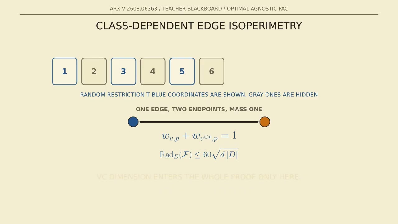
## Key takeaways - [00:00](https://www.youtube.com/watch?v=RGbnAsZlp5I&t=0s) PAC learning theory has long understood the extreme regimes of clean data (d/n) and noisy agnostic data (sqrt(d/n)), but high-probability interpolation across intermediate noise levels L* remained open for thirty years. - [00:41](https://www.youtube.com/watch?v=RGbnAsZlp5I&t=41s) The learning setting evaluates an improper predictor against a hypothesis class of VC dimension d, with the objective of minimizing excess risk above the best-in-class risk L*. - [01:38](https://www.youtube.com/watch?v=RGbnAsZlp5I&t=98s) The Devroye–Györfi–Lugosi lower bound dictates that any agnostic PAC learner must suffer an excess risk scaling with both sqrt(L*(d + log(1/delta))/n) and (d + log(1/delta))/n. - [02:25](https://www.youtube.com/watch?v=RGbnAsZlp5I&t=145s) Empirical Risk Minimization incurs extra logarithmic penalties, while recent state-of-the-art work by Hanneke, Larsen, and Zhivotovskiy (2024) still retained an unwanted log^5(n/d) factor. - [02:25](https://www.youtube.com/watch?v=RGbnAsZlp5I&t=145s) Existing near-realizable one-inclusion rules place a coefficient strictly greater than 1 on L*, making them unusable for a unified agnostic theorem valid across all noise levels. - [03:13](https://www.youtube.com/watch?v=RGbnAsZlp5I&t=193s) Leave-one-out prediction can be represented geometrically as directing edges on the Boolean hypercube {-1, +1}^n, where prediction error on held-out coordinates corresponds to vertex out-degree. - [04:04](https://www.youtube.com/watch?v=RGbnAsZlp5I&t=244s) A novel class-dependent edge isoperimetric lemma uses random restrictions to bound edge capacity by the Hamming distance plus a localized Rademacher width of 60*sqrt(dm), where VC dimension d enters the proof. - [05:05](https://www.youtube.com/watch?v=RGbnAsZlp5I&t=305s) Applying Hall's Marriage Theorem directs cube edges within allocated vertex capacities, securing a leave-one-out bound that preserves an exact leading coefficient of 1 on empirical risk. - [05:57](https://www.youtube.com/watch?v=RGbnAsZlp5I&t=357s) Because one-inclusion rules can exhibit heavy tails, suffix averaging across intermediate training steps is introduced to convert expected bounds into exponential tail bounds with log(1/delta) dependence. - [05:57](https://www.youtube.com/watch?v=RGbnAsZlp5I&t=357s) Forward and reverse martingales couple leave-one-out errors with true population excess risk, allowing martingale variance to scale cleanly with the noise level L*. - [06:53](https://www.youtube.com/watch?v=RGbnAsZlp5I&t=413s) Majority voting cannot be used to convert real-valued suffix scores into binary predictions, as doubling the error would replace the critical leading coefficient of 1 on L* with 2. - [06:53](https://www.youtube.com/watch?v=RGbnAsZlp5I&t=413s) The authors instead use nested-threshold validation on an independent holdout set, utilizing the low metric entropy of nested sets to avoid paying any log(n) penalty. - [07:43](https://www.youtube.com/watch?v=RGbnAsZlp5I&t=463s) The complete algorithm partitions n samples into thirds (k = floor(n/3)), using 2k - 1 points for suffix-averaged training and k points for validation thresholding. - [07:43](https://www.youtube.com/watch?v=RGbnAsZlp5I&t=463s) The learner achieves the minimax-optimal bound without needing L* or delta as inputs, matching the theoretical lower bound up to a universal constant bounded by 7e8.

## Detailed walkthrough ### [00:00](https://www.youtube.com/watch?v=RGbnAsZlp5I&t=0s) The Missing Middle Rate

The lecture opens on a completely blank blackboard to resolve a thirty-year open question in PAC (Probably Approximately Correct) learning theory. On the left side of the board stands the clean, realizable world where at least one hypothesis in the class makes zero mistakes. On the right side stands the noisy, agnostic world where even the best possible rule in the class is wrong a constant fraction of the time. The standard sample complexity and excess risk extremes for these two worlds have long been understood: clean data requires an excess risk scaling around the VC dimension divided by the sample size ($d/n$), whereas noisy data incurs a much slower square-root rate ($\sqrt{d/n}$).

The catch that confounded researchers for three decades is that no known learning algorithm could interpolate between those two regimes across every intermediate noise level with high probability. That exact gap is settled by the paper under discussion (arXiv:2608.06363, *An Optimal Agnostic PAC Algorithm* by Markus Engelund Mathiasen, Jian Qian, and Nikita Zhivotovskiy).

[00:41](https://www.youtube.com/watch?v=RGbnAsZlp5I&t=41s) Four Core Objects Before Any Theorems

Before diving into formulas, four fundamental mathematical objects must be established on the board: 1. **Hypothesis class $\mathcal{H}$:** A family of allowed binary classification rules, where each rule maps inputs to $\{+1, -1\}$. 2. **VC dimension $d$:** The combinatorial complexity of $\mathcal{H}$, defined as the largest number of points that the class can shatter (label in every possible combination). 3. **Training sample:** An i.i.d. dataset consisting of $n$ labeled pairs. 4. **Risk and optimal risk $L^*$:** The risk of any rule $h$ is simply the probability that it disagrees with the true label on a random draw. The absolute lowest risk achievable by any function within the class $\mathcal{H}$ is denoted as $L^*$.

The algorithm produces a predictor $\hat{h}$, which is allowed to be improper (it does not necessarily have to belong to $\mathcal{H}$). The entire objective of the theory centers on the excess risk—the gap between the risk of $\hat{h}$ and the best-in-class risk $L^*$. Every subsequent equation is strictly a statement bounding this excess risk gap.

[01:38](https://www.youtube.com/watch?v=RGbnAsZlp5I&t=98s) The Devroye–Györfi–Lugosi Sandwich

A common but false initial intuition is that a single uniform rate should govern excess risk across all regimes. In reality, nature enforces two distinct behaviors depending on noise: - When $L^* = 0$, the minimax excess risk is $\mathcal{O}(d/n)$. - When $L^*$ is bounded away from zero by a constant, the minimax excess risk scales as $\mathcal{O}(\sqrt{d/n})$.

Luc Devroye, László Györfi, and Gábor Lugosi established a matching lower bound showing that any learner can be forced, with probability at least $\delta$, to suffer an excess risk of at least:

$$\Omega\left(\sqrt{\frac{L^*(d + \log(1/\delta))}{n}} + \frac{d + \log(1/\delta)}{n}\right)$$

Because this lower bound dictates the best possible performance at any noise level, "the sandwich is the truth." The longstanding open problem was discovering an algorithm whose performance matches this lower bound from above, without paying unnecessary penalty factors.

[02:25](https://www.youtube.com/watch?v=RGbnAsZlp5I&t=145s) Why Existing Learners Miss the Target

Standard and state-of-the-art algorithms repeatedly fail to hit this exact sandwich: - **Empirical Risk Minimization (ERM):** The textbook strategy of choosing the hypothesis with the fewest training errors incurs suboptimal overheads. It pays an extra $\sqrt{\log(1/L^*)}$ factor in the slow square-root term and an extraneous $\log(n/d)$ factor in the fast rate term. - **Recent progress (Hanneke, Larsen, and Zhivotovskiy, 2024):** While getting significantly closer, their bound still carried an unwanted $\log^5(n/d)$ factor on the fast term. - **Near-realizable One-Inclusion Rules:** Other variants achieve optimal rates only in the tiny corner where $L^* \le d/n$. Crucially, they place a leading coefficient strictly greater than $1$ directly on $L^*$. While that constant multiplier is harmless when $L^*$ is vanishingly small, having any coefficient larger than one on $L^*$ completely destroys the bound when trying to prove a single agnostic theorem valid across all noise levels.

The mission of the paper is to eliminate every single one of these extraneous logarithmic factors and oversized leading coefficients.

[03:13](https://www.youtube.com/watch?v=RGbnAsZlp5I&t=193s) Leave-One-Out Prediction on the Boolean Cube

To build the proof, the continuous or high-dimensional input space is temporarily set aside in favor of a purely discrete combinatorial structure: the Boolean hypercube $\{-1, +1\}^n$. The vector of $n$ observed labels forms a single vertex on this cube. The hypothesis class $\mathcal{H}$ traces out a restricted subset of vertices, labeled $F$. For any arbitrary label vector $v$, walking to the nearest vertex in $F$ flips a certain number of coordinates; this count is the Hamming distance $\rho(v)$.

Leave-one-out cross-validation translates directly into graph geometry on the cube: - To leave out coordinate $i$, hide coordinate $i$ and consider the unique cube edge connecting the two labelings that differ only at index $i$. - Predicting the missing label corresponds to directing that edge. - The predictor makes an error precisely when the true completion corresponds to the tail of the directed edge. - Consequently, counting leave-one-out prediction errors across all coordinates is mathematically identical to measuring the out-degree of the vertex.

[04:04](https://www.youtube.com/watch?v=RGbnAsZlp5I&t=244s) Class-Dependent Edge Isoperimetry via Random Restrictions

Classical edge isoperimetric inequalities on the Boolean cube bound how many edges a subset can contain purely as a function of the subset's volume. That standard tool operates at the wrong scale here, because subsets located far away from the hypothesis set $F$ should naturally be permitted to contain more edges.

The authors resolve this by developing a new lemma based on fractional edge weights generated through random restrictions: - Let $T$ be a random restriction where each coordinate is independently observed or hidden with probability $1/2$. - On the visible coordinates, fit the nearest hypothesis in $F$. - The hidden coordinate will disagree with that fitted hypothesis on exactly one of the edge's two endpoints, meaning the fractional weights assigned to the two endpoints sum to exactly $1$. - Summing these weights toward any vertex costs at most the Hamming distance $\rho$ to $F$ plus the Rademacher width of the projected class. - The projection's Rademacher width is bounded by at most $60\sqrt{d \cdot m}$, where $m$ is the number of coordinates. This localized width calculation is the only place in the entire proof where the VC dimension $d$ actually enters.

[05:05](https://www.youtube.com/watch?v=RGbnAsZlp5I&t=305s) Cube Orientation via Hall's Marriage Theorem

Once it is established that every induced subgraph contains at most as many edges as the sum of its Hamming distances and localized Rademacher widths, Hall's Marriage Theorem provides an orientation of the cube edges: - Imagine each vertex as a bucket with an allocated capacity of $\rho + 120\sqrt{d\rho} + 7200d$. - Hall's theorem guarantees that every internal edge can be directed into an endpoint's bucket without overflowing any bucket's capacity. - Dividing through by the sample size $n$ directly yields the long-sought leave-one-out risk bound:

$$\text{Leave-one-out risk} \le \hat{L}^* + 120\sqrt{\frac{d\hat{L}^*}{n}} + \mathcal{O}\left(\frac{d}{n}\right)$$

where $\hat{L}^*$ is the empirical optimal risk. The pivotal feature of this formula is the leading term: the coefficient on $\hat{L}^*$ is exactly $1$. Preserving that exact coefficient of one without any inflation is the single reason the agnostic interpolation survives.

[05:57](https://www.youtube.com/watch?v=RGbnAsZlp5I&t=357s) Suffix Averaging for High-Probability Guarantees

Although the cube orientation establishes an optimal bound in expectation, it does not complete the task. Certain one-inclusion prediction rules that achieve optimal expected risk have heavy tails that decay no faster than Markov's inequality, preventing a naive leave-one-out bound from yielding the required logarithmic confidence term $\log(1/\delta)$.

To convert expected guarantees into exponential tail bounds, the paper adopts *suffix averaging*: 1. For every index $t$ ranging from $k$ through $2k - 1$, train a symmetrized score function using the first $t$ data points. 2. Average these intermediate scoring functions together. 3. Apply a reverse martingale that removes sample points backward; permutation invariance converts the leave-one-out guarantees into realized held-out test errors. 4. Apply a forward martingale that adds points forward to couple those held-out errors with the true population excess risk.

Because the variance of these martingales is allowed to scale directly with the underlying noise $L^*$, the full interpolation emerges equipped with a clean $\log(1/\delta)$ dependency.

[06:53](https://www.youtube.com/watch?v=RGbnAsZlp5I&t=413s) Nested-Threshold Validation Over Majority Voting

A subtle hurdle remains: the suffix-averaged score outputs a real-valued prediction in $[-1, +1]$ rather than a crisp binary label. In realizable PAC learning ($L^* = 0$), taking a majority vote of real-valued ensemble predictions at most doubles the total error, which is completely benign when zero doubled is still zero. In the agnostic setting where $L^* > 0$, however, doubling the error would replace the leading coefficient of $1$ with a $2$, destroying the optimal rate.

The paper bypasses majority voting using a quieter validation technique: - Reserve an independent validation block of data. - Sweep a scalar threshold across the real-valued suffix scores. - The resulting candidate binary classifiers form two nested families of sets: predictions strictly above a reference cut, and predictions strictly below it. - Because nested disagreement sets possess very small local metric entropy, running Empirical Risk Minimization across this one-dimensional family incurs zero extra $\log n$ penalty. - The outcome is a fully deterministic binary predictor in $\{+1, -1\}$.

```mermaid flowchart TD accTitle: Three-Block Optimal PAC Learner Architecture accDescr: Pipeline showing data split into three blocks followed by suffix averaging, nested thresholding, and final binary predictor.

subgraph DataSplit["Data Partitioning (Sample size n)"] D1["Block 1 & 2: First 2k - 1 points\n(k = floor(n/3))"] D2["Block 3: Next k points\n(Validation set)"] end

subgraph Block1["Cube Orientation & Suffix Averaging"] O["Orient Cube via Hall's Theorem\n(Leave-one-out out-degree)"] S["Suffix Averaging over t = k to 2k - 1\n(Scores in [-1, +1])"] O --> S end

subgraph Block2["Threshold Validation"] T["Nested Threshold Cuts\n(Low local entropy class)"] ERM["ERM Validation over Cuts\n(Avoids majority vote doubling)"] T --> ERM end

Out["Deterministic Classifier\nOptimal excess risk rate"]

D1 --> Block1 Block1 --> T D2 --> ERM ERM --> Out ```

[07:43](https://www.youtube.com/watch?v=RGbnAsZlp5I&t=463s) The Interpolation Closes as a Theorem

The overall learning pipeline operates by splitting the total sample of size $n$ into thirds, setting $k = \lfloor n/3 \rfloor$: - The first $2k - 1$ samples train the suffix-averaged real-valued score via the cube orientation mechanism. - The subsequent $k$ samples serve exclusively as the holdout validation set to select the optimal threshold.

Remarkably, this learner requires no prior knowledge of the true noise level $L^*$ and does not need to know the target failure probability $\delta$. With probability at least $1 - \delta$, the risk of the learned classifier satisfies:

$$\text{Risk}(\hat{h}) \le L^* + C \left(\sqrt{\frac{L^*(d + \log(1/\delta))}{n}} + \frac{d + \log(1/\delta)}{n}\right)$$

The explicit constant $C$ produced in the constructive proof is roughly $2 \times 10^8$ (simplified in the paper's abstract to $7 \times 10^8$ after absorbing log factors). While that constant is astronomically large and completely unoptimized, the functional shape of the bound matches the lower bound down to the universal constant. The intermediate rate between clean and noisy learning is not an artificial compromise; it is a fundamental sandwich, and theory now possesses an explicit algorithm achieving it.

- **Sample partition:** $k = \lfloor n/3 \rfloor$; $2k - 1$ points for training, $k$ points for threshold selection. - **Explicit constants:** Bucket out-degree capacity includes $120\sqrt{d\rho}$ and constant $7200d$; overall excess risk constant is bounded by $7 \times 10^8$. - **Parameter-free:** The learner adapts automatically without receiving $L^*$ or $\delta$ as inputs.

## Notable quotes > [00:00](https://www.youtube.com/watch?v=RGbnAsZlp5I&t=0s) PAC stands for Probably Approximately Correct. Leslie Valiant introduced the name in 1984 as a model of what it means to learn from a finite sample. — Xiaol.x

> [00:00](https://www.youtube.com/watch?v=RGbnAsZlp5I&t=0s) For thirty years the missing piece was the interpolation between them: a high-probability bound that tracks the best-in-class risk L* at every noise level. — Xiaol.x

> [01:38](https://www.youtube.com/watch?v=RGbnAsZlp5I&t=98s) the sandwich is the truth. — Xiaol.x

> [03:13](https://www.youtube.com/watch?v=RGbnAsZlp5I&t=193s) To leave out coordinate i, hide coordinate i and consider the unique cube edge connecting the two labelings that differ only at index i. — Xiaol.x

> [03:13](https://www.youtube.com/watch?v=RGbnAsZlp5I&t=193s) counting leave-one-out prediction errors across all coordinates is mathematically identical to measuring the out-degree of the vertex. — Xiaol.x

> [04:04](https://www.youtube.com/watch?v=RGbnAsZlp5I&t=244s) This localized width calculation is the only place in the entire proof where the VC dimension d actually enters. — Xiaol.x

> [05:05](https://www.youtube.com/watch?v=RGbnAsZlp5I&t=305s) Preserving that exact coefficient of one without any inflation is the single reason the agnostic interpolation survives. — Xiaol.x

> [06:53](https://www.youtube.com/watch?v=RGbnAsZlp5I&t=413s) In realizable PAC learning (L* = 0), taking a majority vote of real-valued ensemble predictions at most doubles the total error, which is completely benign when zero doubled is still zero. — Xiaol.x

> [06:53](https://www.youtube.com/watch?v=RGbnAsZlp5I&t=413s) Because nested disagreement sets possess very small local metric entropy, running Empirical Risk Minimization across this one-dimensional family incurs zero extra log n penalty. — Xiaol.x

> [07:43](https://www.youtube.com/watch?v=RGbnAsZlp5I&t=463s) The learner never needs L* or delta. The constant is huge and unoptimized. The shape is optimal. — Xiaol.x

> [07:43](https://www.youtube.com/watch?v=RGbnAsZlp5I&t=463s) The intermediate rate between clean and noisy learning is not an artificial compromise; it is a fundamental sandwich, and theory now possesses an explicit algorithm achieving it. — Xiaol.x

## Mentioned Leslie Valiant, Markus Engelund Mathiasen, Jian Qian, Nikita Zhivotovskiy, Luc Devroye, László Györfi, Gábor Lugosi, Steve Hanneke, Kasper Green Larsen, Philip Hall, Xiaol.x, An Optimal Agnostic PAC Algorithm (arXiv:2608.06363), Aarhus University, University of Hong Kong (HKU), UC Berkeley

## Video description PAC stands for Probably Approximately Correct. Leslie Valiant introduced the name in 1984 as a model of what it means to learn from a finite sample. Approximately correct means the classifier’s error is close to the best rule in the class. Probably means that guarantee holds with high probability over the random sample, at least 1 minus delta. A PAC bound is not “this rule is always perfect.” It is: with high probability, the excess risk is at most some function of the sample size n, the VC dimension d, and the noise level L*.

PAC theory already knew two extremes. In a clean world, excess risk is about d/n. In a noisy world, it is about sqrt(d/n). For thirty years the missing piece was the interpolation between them: a high-probability bound that tracks the best-in-class risk L* at every noise level.

This blackboard lesson teaches arXiv 2608.06363, An Optimal Agnostic PAC Algorithm, by Markus Engelund Mathiasen, Jian Qian, and Nikita Zhivotovskiy. Empirical risk minimization pays extra logs. A 2024 bound still carries log^5(n/d). Near-realizable one-inclusion rules put a coefficient larger than one on L*. This paper closes the gap, matching the Devroye–Györfi–Lugosi lower bound up to a universal constant.

The board starts blank. We name every object before any theorem, then build three classroom objects: a risk thermometer, a Boolean cube whose hidden edge is leave-one-out, and a three-block learner — cube orientation, suffix averaging, nested-threshold validation.

Paper: https://arxiv.org/abs/2608.06363 Authors: Markus Engelund Mathiasen (Aarhus), Jian Qian (HKU), Nikita Zhivotovskiy (Berkeley)

Chapters 00:00 The missing middle rate 00:41 Name every object before any theorem 01:38 The sandwich you are not allowed to beat 02:25 Why nearby algorithms miss 03:13 Leave-one-out is a cube edge 04:04 Class-dependent edge isoperimetry 05:05 Hall orients the cube with coefficient one 05:57 Suffix averaging for high probability 06:53 Do not majority-vote the noise away 07:43 The interpolation is now a theorem

The learner never needs L* or delta. The constant is huge and unoptimized. The shape is optimal.

[Source](https://www.youtube.com/watch?v=RGbnAsZlp5I)

中文简报

Mathiasen、Qian 与 Zhivotovskiy 弥合 PAC 学习率 30 年理论差距通过将保持最小风险单位系数的布尔立方体定向与后缀平均及嵌套阈值验证相结合，该三块学习算法在所有噪声水平下均匹配了极小化极大超额风险下界，且不产生对数开销。尽管 PAC 学习理论在极端的完全可实现状态（$O(d/n)$）与不可知状态（$O(\sqrt{d/n})$）下具有紧确界，但寻找一种能以大概率在所有噪声水平下于两者之间完成插值的算法一直是一项悬而未决的挑战。本讲座概述了一种最优学习算法，该算法将数据投影到布尔超立方体上，并利用霍尔婚姻定理实现了在经验风险上具有严格为 1 的前导系数的留一法误差界。为了将该期望界推广至高概率情形，该学习算法将鞅上的后缀平均与嵌套阈值验证步骤相结合，完全避免了传统多数投票所带来的风险翻倍惩罚。由此构建的三块算法能够自适应匹配下界，无需对噪声水平或目标置信度具有先验认知。 Mathiasen、Qian 和 Zhivotovskiy（arXiv 2608.06363）通过构建一种在所有噪声水平下均匹配 Devroye–Györfi–Lugosi 下界的最优不可知 PAC 学习算法，解决了一个长达 30 年的开放性问题。 (0:00) 该几何证明机制通过霍尔婚姻定理将留一法误差映射到布尔超立方体上的边定向，从而在经验最小风险上确保了严格为 1 的关键前导系数。 (5:05) 对训练前缀进行后缀平均，并结合逆鞅与前向鞅，将厚尾留一法估计转化为了高概率 Bernstein 界。 (5:57) 该算法通过在留出数据块上采用嵌套阈值验证，规避了多数投票的风险翻倍惩罚，在不产生对数开销的情况下实现了对噪声和置信度的完全自适应。 (6:53)

Reading summary

A paper by Markus Engelund Mathiasen, Jian Qian, and Nikita Zhivotovskiy resolves a thirty-year open problem in PAC learning by presenting an algorithm that achieves optimal excess risk bounds across every noise level without prior knowledge of the optimal risk or confidence parameters. The Excess Risk Interpolation Problem (1:38) In PAC learning theory, sample complexity historically diverged into two extremes: a fast excess risk rate of approximately $d/n$ when data is realizable ($L^* = 0$), and a slower square-root rate of $\mathcal{O}(\sqrt{d/n})$ when the best-in-class risk $L^*$ is bounded away from zero. A matching lower bound by Luc Devroye, László Györfi, and Gábor Lugosi established that any learner can be forced to experience excess risk of at least $\Omega(\sqrt{L^*(d + \log(1/\delta))/n} + (d + \log(1/\delta))/n)$. Matching this lower bound across all noise levels simultaneously had eluded researchers for decades. Standard Empirical Risk Minimization introduces extraneous logarithmic overheads, including a $\sqrt{\log(1/L^*)}$ penalty in the slow term and a $\log(n/d)$ factor in the fast term. Recent work by Hanneke, Larsen, and Zhivotovskiy (2024) narrowed the gap but retained a $\log^5(n/d)$ factor. Meanwhile, near-realizable one-inclusion rules that succeed when $L^* \le d/n$ impose a leading constant strictly greater than 1 on $L^*$, which invalidates universal agnostic guarantees when $L^*$ is large. Hypercube Geometry and Edge Orientation (3:13) The authors analyze leave-one-out prediction on the Boolean hypercube $\{-1, +1\}^n$, where the hypothesis class $\mathcal{H}$ corresponds to a subset of vertices $F$, and the Hamming distance to $F$ is denoted by $\rho(v)$. Leaving out a coordinate is equivalent to traversing a cube edge between labelings that differ only at that coordinate. Because prediction errors occur when the true completion sits at the tail of a directed edge, counting leave-one-out errors corresponds to calculating a vertex's out-degree. To control out-degrees, the proof establishes an edge isoperimetric lemma tailored to $F$ using random restrictions, showing that assigned edge weights sum to at most $\rho$ plus the localized Rademacher width of the projected class. Bounding this width by $60\sqrt{d \cdot m}$ provides the only step where the VC dimension $d$ enters. Applying Hall's Marriage Theorem then directs internal edges into vertex buckets with capacities of $\rho + 120\sqrt{d\rho} + 7200d$. Normalizing by the sample size $n$ gives a leave-one-out risk bound of $\hat{L}^* + 120\sqrt{d\hat{L}^*/n} + \mathcal{O}(d/n)$, preserving an exact leading coefficient of 1 on the empirical optimal risk $\hat{L}^*$. Exponential Concentration Through Suffix Averaging (5:57) While cube orientation bounds expected leave-one-out risk, standard one-inclusion predictions exhibit heavy tails governed only by Markov's inequality, which fails to yield exponential $\log(1/\delta)$ concentration. To overcome this limitation, the algorithm implements suffix averaging over sample sizes $t$ from $k$ to $2k - 1$, generating and averaging symmetrized scoring functions. The resulting estimator is analyzed using a pair of martingales. A reverse martingale removes data points backward, relying on permutation invariance to equate leave-one-out guarantees with held-out test errors. A forward martingale then adds data points forward to couple these test errors to the population excess risk. Because the martingale variance scales directly with the noise level $L^*$, the formulation yields high-probability bounds with the target $\log(1/\delta)$ term. Nested-Threshold Validation (6:53) Suffix averaging yields real-valued scores in $[-1, +1]$ rather than binary predictions. In agnostic settings, standard majority voting fails because it doubles the overall error, replacing the critical leading coefficient of 1 with a 2 and ruining the rate. The algorithm circumvents voting by reserving an independent validation block of $k = \lfloor n/3 \rfloor$ samples to evaluate scalar thresholds applied to the suffix scores. Sweeping this threshold creates two nested families of classifier cuts. Because nested disagreement sets have low local metric entropy, Empirical Risk Minimization over this one-dimensional candidate family incurs no additional $\log n$ sample penalty. The procedure produces a deterministic binary classifier whose excess risk matches the Devroye–Györfi–Lugosi lower bound without requiring $L^*$ or $\delta$ as inputs. The resulting excess risk bound matches the minimax lower bound up to a universal constant, formally settling the agnostic PAC interpolation question. However, the explicit constant $C$ derived in the constructive proof is astronomically large—roughly $2 \times 10^8$, simplified to $7 \times 10^8$ after absorbing logarithmic factors—leaving practical constant optimization as an open theoretical refinement.

Source quotes

[0:00] Xiaol.x: PAC stands for Probably Approximately Correct. Leslie Valiant introduced the name in 1984 as a model of what it means to learn from a finite sample. [0:00] Xiaol.x: For thirty years the missing piece was the interpolation between them: a high-probability bound that tracks the best-in-class risk L* at every noise level. [1:38] Xiaol.x: the sandwich is the truth. [3:13] Xiaol.x: To leave out coordinate i, hide coordinate i and consider the unique cube edge connecting the two labelings that differ only at index i. [3:13] Xiaol.x: counting leave-one-out prediction errors across all coordinates is mathematically identical to measuring the out-degree of the vertex. [4:04] Xiaol.x: This localized width calculation is the only place in the entire proof where the VC dimension d actually enters. [5:05] Xiaol.x: Preserving that exact coefficient of one without any inflation is the single reason the agnostic interpolation survives. [6:53] Xiaol.x: In realizable PAC learning (L* = 0), taking a majority vote of real-valued ensemble predictions at most doubles the total error, which is completely benign when zero doubled is still zero. [6:53] Xiaol.x: Because nested disagreement sets possess very small local metric entropy, running Empirical Risk Minimization across this one-dimensional family incurs zero extra log n penalty. [7:43] Xiaol.x: The learner never needs L* or delta. The constant is huge and unoptimized. The shape is optimal. [7:43] Xiaol.x: The intermediate rate between clean and noisy learning is not an artificial compromise; it is a fundamental sandwich, and theory now possesses an explicit algorithm achieving it.

Original transcript

[0:00] Today we settle a 30-year classroom [0:02] question in PAC learning. Look at this [0:05] blank board. On the left, I will keep a [0:08] clean world where some rule in the class [0:11] never makes a mistake. On the right, I [0:14] will keep a noisy world where even the [0:16] best rule in the class is wrong a [0:17] constant fraction of the time. You [0:19] already know the two extremes. Clean [0:22] data needs about VC dimension over N [0:24] samples. Noisy data needs a square root. [0:29] Here is the catch. Nobody had a learner [0:33] that interpolates those two rates [0:36] at every noise level with high [0:38] probability. That is the paper. [0:42] Before any formula, we need four [0:44] objects. First, a hypothesis class H, a [0:47] family of allowed binary rules, each [0:50] answering plus one or minus one. Second, [0:54] it's VC dimension D, the largest number [0:58] of points the class can label in every [1:00] possible way. [1:01] Third, an IID sample of N labeled pairs. [1:06] Fourth, risk. The risk of a rule H is [1:11] simply the probability it disagrees with [1:13] the random label. Mark the lowest [1:16] possible risk inside the class as L [1:18] star. [1:19] The learner outputs some hat H, which [1:23] need not even sit inside H. [1:26] The gap between its risk and L star is [1:28] the excess. Every [1:31] later equation is only a statement about [1:36] this gap. [1:39] You might expect one rate to rule them [1:41] all. That is the first false intuition. [1:44] When L star is zero, the optimal excess [1:48] is ordered D over N. When L star sits a [1:52] constant away from zero, the optimal [1:55] excess is order square root of D over N. [1:58] Devroye, Györfi, and Lugosi already [2:00] proved a matching lower bound that [2:02] interpolates the two. With probability [2:04] at least delta, some world forces excess [2:07] at least a constant times square root of [2:09] L star times D plus log one over delta [2:13] over N plus that same complexity over N. [2:18] So, the sandwich is the truth. [2:21] The open problem was the matching upper [2:24] bound. [2:25] Uh [2:26] empirical risk minimization, the obvious [2:29] pick the fewest training mistakes rule [2:31] does not hit this sandwich. It pays a [2:33] square root of log one over L star in [2:36] the slow term and a log N over D in the [2:39] fast term. In 2024, Haneke, Larsen, and [2:44] Zhivotovsky got much closer, but they [2:47] still carry a log to the fifth of N over [2:50] D on the fast term. Other one inclusion [2:53] rules are optimal only when L star is [2:55] already as small as D over N, and they [2:58] put a coefficient larger than one on L [3:00] star itself. Harmless in that tiny noise [3:03] corner. Fatal if you want one theorem at [3:07] every noise level. The paper's job is to [3:10] kill those extra factors. [3:13] >> [sighs and gasps] [3:14] >> Now, look at the object that will carry [3:16] the proof. Forget the original input [3:19] space for a moment. The N labels are a [3:21] vertex of the Boolean cube. Every [3:24] coordinate is plus one or minus one. The [3:28] hypothesis class traces only some of [3:30] those vertices. Call that subset F. Um [3:34] from any labeling V, walk to the nearest [3:37] vertex of F. [3:39] Um the number of flipped coordinates is [3:42] the Hamming distance row of V. Leave one [3:45] out means this. Hide coordinate I. Look [3:49] at the unique cube edge that flips only [3:52] I and predict the missing label. You are [3:55] wrong exactly when the true completion [3:58] is the tail of that edge. So, a leave [4:01] one out error count is an out degree. [4:05] Classical cube isoperimetry tree bounds [4:09] how many edges a set can hide using only [4:11] the set size. That is the wrong scale [4:14] here because a set far from F should be [4:16] allowed more edges. The new lemma builds [4:19] fractional weights on every cube edge. [4:22] Draw a random restriction T. [4:25] Each coordinate is independently shown [4:28] or hidden with probability 1/2. [4:31] On the visible coordinates, pick the [4:33] nearest hypothesis. The hidden [4:35] coordinate disagrees with that fit on [4:39] exactly one of the two end points. So, [4:41] the two weights sum to one. Summing [4:43] weights toward a vertex costs at most [4:47] the Hamming distance to F [4:50] plus a Rademacher width of the [4:52] projection. And that width is at most 60 [4:56] square root of D times the number of [4:58] coordinates. [5:00] That is the only place VC dimension [5:04] enters the whole proof. [5:06] Once every induced subgraph has at most [5:09] as many edges as the sum of Hamming [5:11] distance plus localized width, Hall's [5:14] theorem supplies an orientation. Think [5:16] of each vertex as a bucket whose [5:18] capacity is row plus 120 square root of [5:21] D row plus 7202D. [5:25] Every internal edge can be assigned to a [5:27] bucket without overflow. Divide by N and [5:30] you obtain the leave one out bound the [5:32] field wanted. Leave one out risk is at [5:34] most the empirical optimum plus 120 [5:37] square root of D times that optimum over [5:40] N plus [5:42] a constant times D over N. Look at the [5:46] first term after the empirical optimum. [5:49] The coefficient on L hat star is one. [5:52] That single one is why the interpolation [5:55] can survive. [5:58] You might expect the orientation to [5:59] finish the lecture. Here is the catch. [6:02] Some one inclusion rules that are [6:04] optimal in expectation have tails no [6:07] better than Markov's inequality. [6:09] Um [6:10] so a leave one out bound does not [6:12] automatically give the optimal [6:14] dependence on delta. The paper borrows [6:16] suffix averaging. Train a symmetrized [6:19] score on the first T points for every T [6:23] from K through 2K minus 1. Then average [6:26] those scores. A reverse martingale [6:29] deletes points backward. So permutation [6:32] invariance turns the leave one out bound [6:35] into realized held out errors. A forward [6:38] martingale adds points forward and [6:41] compares those errors with true [6:43] population excess. Because the variance [6:46] is allowed to depend on L star, the [6:49] interpolation reappears with a clean log [6:52] 1 over delta. [6:54] Uh [6:54] >> [sighs] [6:55] >> suffix averaging still outputs a score [6:57] between minus 1 and 1. In the realizable [7:00] case, you can take a majority vote and [7:02] at most double the risk. Doubling is [7:04] harmless when L star is zero. It would [7:07] destroy coefficient 1 when L star is [7:11] positive. [7:13] Um [7:14] so the last move is quieter. Hold out a [7:18] fresh validation block. Slide a [7:20] threshold across the score. The [7:23] resulting binary rules form two nested [7:26] families. Everything above a reference [7:28] cut and everything below. Nested [7:31] disagreement sets have tiny local [7:32] entropy, so empirical risk minimization [7:35] over this threshold class pays no extra [7:37] log n. The output is a deterministic [7:40] plus or minus one classifier. [7:44] Put the three blocks on one pipeline, [7:47] split N into thirds [7:50] with K the floor of N over three, [7:54] build the suffix average score from the [7:56] first 2K minus one points, use the next [8:00] K points only to choose the threshold. [8:03] The learner never looks at L star and [8:06] never looks at delta. [8:08] With probability at least 1 minus delta, [8:11] its risk is L star plus 2 * 10 to the 8 [8:15] * the interpolation. The abstract [8:17] rewrites the log 48 into a still [8:19] universal 7 * 10 to the 8. The constant [8:22] is huge and unoptimized. The shape is [8:24] optimal. [8:26] Take the board with you. The rate [8:28] between clean and noisy is not a [8:29] compromise. It is a sandwich and we now [8:33] have a learner that sits on the [8:35] sandwich.