Researchers Pinpoint Mathematical Limit for LLM Data Repetition

Xiaol.x

Repeating scarce training data beyond the point where marginal signal acquisition is overtaken by noise fitting causes overfitting, making in-domain validation loss the primary predictor of optimal stopping.

AI-assisted summary of When Should LLMs Repeat Training Data? Perplexity, Overfitting & the Math of Optimal Repetition — original source. Check the original for full context.

Source published: 2026-08-20

Key ideas

Data repetition in LLM pretraining operates as a trade-off between signal acquisition and noise memorization, with optimal stopping occurring precisely when the marginal variance penalty of fitting noise overtakes signal gains. (3:06)
Empirical sweeps across sub-2B models revealed that minimum in-domain validation loss exhibits an exceptionally strong Pearson correlation of -0.944 with optimal repetition, whereas unique data fraction showed almost no predictive correlation (r = 0.018). (7:38)
Model scaling alters repetition limits depending on budget design: holding total tokens fixed causes larger models to overfit repeated data earlier, while keeping tokens-per-parameter (TPP) constant allows optimal repetition to scale positively with data size. (6:32)
Domain tolerance varies widely under empirical tests: Math corpora safely endure roughly 5 to 6 passes, Code tolerates 4 to 5, while Wikipedia and Medical data degrade after only 3 to 4 passes. (7:38)

Detailed notes

## Background Published on YouTube by Xiaol.x on August 20, 2026, this LeanAnim video breaks down the research paper 'Scaling Domain Data Repetition in LLM Pretraining' (arXiv:2608.14071). According to the video description, it uses step-by-step mathematical deductions, geometric intuition, and empirical sweeps to explain when repeating scarce, high-quality training data benefits language models versus when it drives overfitting.

## TL;DR The explainer addresses the training paradox where scaling token budgets dilutes scarce specialized corpora, examining how data replay simultaneously reinforces structural signal and accelerates noise memorization. It formalizes this trade-off using a solvable one-coordinate regression model to derive the mathematical stopping point where noise fitting overtakes signal acquisition. The breakdown reconciles conflicting scaling trends by showing that fixed token counts push toward earlier overfitting while fixed tokens-per-parameter (TPP) scaling permits higher repetition, supported by empirical sweeps across math, code, medical, and Wikipedia domains. Finally, it outlines practical proxy-model workflows and a marginal-gain allocation framework for balancing multi-domain data mixtures.

## Atmosphere & style The presentation is intensely analytical, disciplined, and pedagogically precise, unfolding like an advanced graduate-level lecture animated through crisp mathematical derivations. There is a calm, methodical rhythm to the explanation, deliberately stripping away intuitive hand-waving to reveal the exact mechanics of loss curves, risk equations, and parameter ratios. It feels intellectually clarifying and grounded, treating metrics like perplexity as pragmatic diagnostic dashboards while guiding the viewer through an elegant bridge between toy theoretical models and real-world pretraining engineering.

## Bulletin - [03:06](https://www.youtube.com/watch?v=WF2DoGotANI&t=186s) Data repetition in LLM pretraining operates as a trade-off between signal acquisition and noise memorization, with optimal stopping occurring precisely when the marginal variance penalty of fitting noise overtakes signal gains. - [07:38](https://www.youtube.com/watch?v=WF2DoGotANI&t=458s) Empirical sweeps across sub-2B models revealed that minimum in-domain validation loss exhibits an exceptionally strong Pearson correlation of -0.944 with optimal repetition, whereas unique data fraction showed almost no predictive correlation (r = 0.018). - [06:32](https://www.youtube.com/watch?v=WF2DoGotANI&t=392s) Model scaling alters repetition limits depending on budget design: holding total tokens fixed causes larger models to overfit repeated data earlier, while keeping tokens-per-parameter (TPP) constant allows optimal repetition to scale positively with data size. - [07:38](https://www.youtube.com/watch?v=WF2DoGotANI&t=458s) Domain tolerance varies widely under empirical tests: Math corpora safely endure roughly 5 to 6 passes, Code tolerates 4 to 5, while Wikipedia and Medical data degrade after only 3 to 4 passes.

## Key takeaways - [00:00](https://www.youtube.com/watch?v=WF2DoGotANI&t=0s) Scaling total compute dilutes finite specialized domain data unless high-quality tokens are replayed, creating a core paradox between model capacity and domain exposure. - [01:58](https://www.youtube.com/watch?v=WF2DoGotANI&t=118s) Perplexity acts as a dashboard rather than a driver; minimizing held-out negative log-likelihood mathematically yields the exact same optimal repetition count as minimizing perplexity. - [03:06](https://www.youtube.com/watch?v=WF2DoGotANI&t=186s) A solvable one-coordinate regression model shows that each repetition pass contracts the distance to the sample mean by a factor of a, balancing decaying signal error against growing noise-fitting error. - [05:27](https://www.youtube.com/watch?v=WF2DoGotANI&t=327s) The small-noise theorem proves that lowering data noise variance delays the onset of overfitting logarithmically but can never eliminate it entirely. - [06:32](https://www.youtube.com/watch?v=WF2DoGotANI&t=392s) Scaling models with a fixed token count exposes rarer parameters without new data, causing larger models to overfit repeated data sooner beyond a crossover model size. - [06:32](https://www.youtube.com/watch?v=WF2DoGotANI&t=392s) Under constant tokens-per-parameter (TPP) scaling, optimal repetition counts increase with data size, resolving the apparent contradiction with fixed-data scaling. - [07:38](https://www.youtube.com/watch?v=WF2DoGotANI&t=458s) Minimum validation loss is the single strongest predictor of optimal repetition count (r = -0.944), far outperforming model size (r = 0.44) and unique data fraction (r = 0.018). - [07:38](https://www.youtube.com/watch?v=WF2DoGotANI&t=458s) Domain-specific structures exhibit distinct tolerances for repetition, with math enduring up to 6 passes while encyclopedic and medical data degrade after 3 to 4 passes. - [08:47](https://www.youtube.com/watch?v=WF2DoGotANI&t=527s) Existing repetition frameworks like Muennighoff's effective data, Lovelace's capacity penalty, and Sedova's generic regularization capture pieces of repetition dynamics but lack explicit fixed-TPP stopping-point derivations. - [09:58](https://www.youtube.com/watch?v=WF2DoGotANI&t=598s) Performance degradation from repeating domain data remains localized to in-domain evaluations, leaving out-of-domain loss largely unaffected. - [09:58](https://www.youtube.com/watch?v=WF2DoGotANI&t=598s) Learning-rate schedules significantly shift optimal repetition: constant learning rates tolerate more passes, whereas early learning-rate decay causes premature overfitting to sample-specific patterns. - [11:04](https://www.youtube.com/watch?v=WF2DoGotANI&t=664s) A practical proxy-model recipe matches the target model's TPP on a smaller proxy and selects the smallest repetition count statistically indistinguishable from the fitted convex minimum. - [12:06](https://www.youtube.com/watch?v=WF2DoGotANI&t=726s) Token budgets across multiple domains can be dynamically allocated by greedily assigning data blocks based on marginal validation gain per token until the opportunity cost of fresh web data exceeds the gain. - [13:36](https://www.youtube.com/watch?v=WF2DoGotANI&t=816s) The theoretical framework relies on stylized linear regression assumptions with orthogonal one-hot features and Gaussian noise, representing an operational heuristic rather than an unconditional law for deep neural networks.

## Detailed walkthrough ### [00:00](https://www.youtube.com/watch?v=WF2DoGotANI&t=0s) The Data Scarcity Paradox and the Dual Nature of Repetition

The discussion opens with a core paradox in LLM pretraining: valuable corpora like code, math, medical literature, and encyclopedias are finite. As models grow larger, compute-optimal training naturally scales up the total token budget. If a high-quality domain corpus remains fixed in size, its fraction of the training stream continuously shrinks. Consequently, a larger model might ingest more total tokens while seeing proportionally less of the specialized domain data researchers actually care about.

To counteract this dilution, training pipelines often replay the scarce domain data. However, every replay simultaneously triggers two competing forces: it reinforces reusable underlying structure, and it gives the optimizer another opportunity to memorize sample-specific noise. The central problem is not whether data repetition is inherently good or bad, but rather determining the exact point where structural reinforcement stops paying for its own overfitting.

To formulate this mathematically, let $N$ represent the number of model parameters, and let total training tokens be defined as $D_N = \text{TPP} \times N$, where TPP is tokens per parameter. Let $\alpha$ be the fraction of the budget occupied by unique high-quality tokens, giving a unique subset size of $U = \alpha D$. Repeating this subset $E$ times results in $H = E\alpha D$ high-quality token presentations, while the remainder consists of fresh web data $W = (1 - E\alpha)D$. While $\alpha$ determines how many different domain tokens exist, $E$ controls how often the subset returns, and their product $E\alpha$ defines the final domain share. At a fixed model size, every recipe consumes the exact same total token budget; only the data composition shifts.

- **Core Paradox:** Larger model capacity increases total tokens, diluting fixed high-quality corpora unless explicitly replayed. - **Dual Effect of Repetition:** Reinforces generalizable structure while increasing the risk of memorizing sample-specific noise. - **Budget Variables:** $N$ parameters, $D_N = \text{TPP} \times N$ tokens, unique fraction $\alpha$, repetition count $E$, and fresh data remainder $W$.

[01:58](https://www.youtube.com/watch?v=WF2DoGotANI&t=118s) Perplexity as a Dashboard, Not a Mechanism

The paper evaluates held-out token average negative log-likelihood, defined as $L$ minus the average log probability of the correct next token. Perplexity is simply the exponential of loss ($\text{PPL} = \exp(L)$) when natural logarithms are used. Because the exponential function is strictly increasing, the repetition count that minimizes validation loss also minimizes validation perplexity, and a loss change $\Delta L$ multiplies perplexity by $\exp(\Delta L)$.

Crucially, perplexity does not cause the optimal repetition behavior; it is merely the dashboard. The underlying mechanism is the competition between acquiring learning signal and fitting noise. The speakers emphasize evaluating in-domain held-out loss rather than training loss, warning against naively comparing raw loss across domains where tokenizer choices and irreducible domain entropy can distort the baseline. The strong cross-domain correlations observed in the paper serve as robust empirical evidence rather than a universal causal law dictated by perplexity itself.

- **Loss vs. Perplexity:** $\text{PPL} = \exp(L)$; minimizing negative log-likelihood mathematically minimizes perplexity due to strict monotonicity. - **The Dashboard Analogy:** Perplexity reflects performance but does not drive the optimization dynamics. - **Methodological Warning:** Always use in-domain held-out loss and account for domain-specific tokenizers and entropy.

[03:06](https://www.youtube.com/watch?v=WF2DoGotANI&t=186s) The One-Coordinate Solvable Model and Optimal Stopping

To expose the underlying mechanism, the paper replaces the full language model with a solvable one-hot regression problem. Here, a single coordinate $K$ represents a knowledge unit that appears $M$ times in a dataset of $D$ observations, with noisy labels averaging to $\bar{Y}$. Full-batch gradient descent updates this single coordinate according to the recurrence relation:

$$\theta_{r+1} = \theta_r - \frac{M}{D}(\theta_r - \bar{Y})$$

Starting from zero, the recurrence solves exactly to $\theta_r = (1 - a^r)\bar{Y}$, where $a = 1 - \frac{M}{D}$.

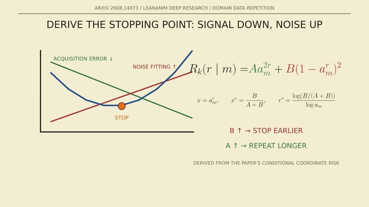
Repetition acts as a contraction dial, where each extra optimization pass multiplies the remaining distance to the sample mean by $a$. Conditioning on the count $M$, the coordinate's expected population error takes the quadratic form:

$$\mathcal{R}(r|m) = A a^{2r} + B(1 - a^r)^2$$

In this formulation, $A$ represents the signal energy still not acquired, while $B = p_k \sigma^2 / m$ represents the variance of the sample mean weighted by coordinate frequency. The first term decreases with repetition as signal is absorbed, while the second term rises as the fitted estimate approaches the noisy sample mean.

```mermaid flowchart LR subgraph Dynamics ["Repetition Dynamics"] A["Signal Energy (A a^2r)"] -->|"Decreases with passes"| C["Total Population Error R(r|m)"] B["Noise Fitting (B(1 - a^r)^2)"] -->|"Increases with passes"| C end accTitle: Repetition Dynamics Flowchart accDescr: Diagram showing how signal energy decreases and noise fitting increases as repetition passes accumulate, combining into the total population error. ```

Setting $x = a^r$ transforms the error equation into $\mathcal{R}(x) = A x^2 + B(1 - x)^2$. Differentiating yields the optimal stopping point:

$$x^* = \frac{B}{A + B}$$

$$r^* = \frac{\log\left(\frac{B}{A + B}\right)}{\log(a)}$$

More noise raises $B$ and moves the stopping point earlier, whereas a cleaner signal raises $A$ and makes additional passes worthwhile for a longer duration.

- **Contraction Dial:** Repetition shrinks the distance to the sample mean by a factor of $a^r$ per pass. - **Error Tradeoff:** Signal acquisition error decreases exponentially while noise-fitting error increases toward the noisy sample mean. - **Optimal Stop:** Determined by the relative weights of noise ($B$) and unacquired signal ($A$).

[05:27](https://www.youtube.com/watch?v=WF2DoGotANI&t=327s) The Complete Population-Risk Equation and the Small-Noise Theorem

Expanding the scalar story across every represented knowledge unit yields the paper's complete population-risk equation, which consists of three distinct terms. First, coordinates beyond model capacity represent unrepresented knowledge that longer training cannot recover. Second, the knowledge acquisition error scales with $k^{-\beta}$ times the expected contraction $a_m^{2r}$, confirming that it decreases with repeated optimization. Third, the noise fitting error contains $\sigma^2 (1 - a_m^r)^2 / m$, showing that it increases as optimization proceeds.

The optimal stopping time is precisely the earliest $r$ where the marginal variance penalty overtakes the marginal signal benefit. This framework naturally explains the small noise theorem: as noise variance $\sigma^2$ approaches zero, the optimal repetition count grows logarithmically according to $\log(1/\sigma^2) / (-\log(1 - a/d))$. Lower noise delays overfitting but does not eliminate it entirely.

- **Three Risk Components:** Unrepresented capacity, decreasing acquisition error, and increasing noise-fitting error. - **Stopping Criterion:** Training stops when the marginal variance penalty exceeds the marginal signal benefit. - **Small-Noise Limit:** Reducing data noise delays overfitting but cannot abolish it completely.

[06:32](https://www.youtube.com/watch?v=WF2DoGotANI&t=392s) Fixed Data Versus Fixed Tokens-Per-Parameter Scaling

The paper introduces a crucial experimental control regarding model scaling. If total training tokens $D$ remain fixed while parameter count $N$ grows, the model exposes rarer coordinates without receiving additional observations. Beyond a critical crossover model size, the paper proves that the optimal stopping time cannot increase and may actually decrease, mathematically validating the warning that larger models overfit repeated data sooner.

However, practical scaling laws usually maintain an approximately constant tokens-per-parameter ($\text{TPP}$) ratio, meaning $D$ grows proportionally with $N$. In this regime, when $D/N$ approaches a positive constant, the optimal repetition count scales positively with data size. Consequently, the apparent contradiction resolves: capacity alone pushes toward earlier stopping, whereas capacity paired with proportional new data pushes toward later stopping. Researchers must never transfer a repetition rule across scales without accounting for changes in $D/N$.

- **Fixed-Token Danger:** Holding $D$ constant while scaling $N$ causes larger models to overfit repeated data much sooner. - **Proportional Scaling:** Maintaining constant tokens per parameter ($\text{TPP}$) allows optimal repetition counts to grow with scale. - **Rule of Thumb:** Always evaluate how $D/N$ shifts before transferring repetition heuristics between different model sizes.

[07:38](https://www.youtube.com/watch?v=WF2DoGotANI&t=458s) Empirical Sweep and Correlation Analysis

The authors conducted empirical sweeps across four domains, four model sizes ranging from 348 million to 1.85 billion parameters, three unique data fractions, and repetition counts from 1 through 7. For every configuration, they fitted a quadratic loss curve $\hat{L}(E) = AE^2 + BE + C$ and estimated the optimal repetition count $E^* = -B / (2A)$.

Statistical analysis reveals that unique data fraction is not the strongest predictor; rather, the minimum in-domain validation loss shows an exceptionally strong Pearson correlation of $-0.944$ with estimated optimal repetition. Model size exhibits a weaker positive correlation of $0.44$, while unique fraction is nearly flat at $0.018$. Across the tested grid, math tolerates roughly 5 to 6 passes, code about 4 to 5, and Wikipedia and medical domains about 3 to 4 passes, though these represent bounded observations rather than universal physical constants.

- **Experimental Grid:** 4 domains, 4 model sizes (348M to 1.85B parameters), 3 unique fractions, and repetition counts 1–7. - **Key Correlation:** In-domain validation loss correlates strongly ($r = -0.944$) with optimal repetition. - **Domain Tolerances:** Math ($\sim 5\text{--}6$), Code ($\sim 4\text{--}5$), Wikipedia and Medical ($\sim 3\text{--}4$).

[08:47](https://www.youtube.com/watch?v=WF2DoGotANI&t=527s) Comparison with Related Repetition Frameworks

To contextualize their findings, the speakers examine three related theoretical lenses from recent literature. Muennighoff and colleagues replace raw repeated tokens with effective data, treating early repeats almost like fresh data while later repeats saturate due to diminishing returns, though this model lacks an explicit rising overfitting loss term. Lovelace and colleagues introduce an explicit penalty proportional to repetition raised to a power, scaled by the ratio of model capacity to unique data, capturing the dual nature of repeated tokens being both useful and costly. Sedova and colleagues study scarce target data mixed with abundant generic data, where the unsaturated generic data term acts as regularization and permits 15 to 20 target repetitions in specific settings.

The present paper distinguishes itself through a fixed-TPP, cross-scale per-domain sweep combined with a precise stopping-time explanation governing how and why the optimum shifts.

- **Muennighoff Effective Data:** Models diminishing returns of repeats but omits the rising overfitting loss. - **Lovelace Penalty Model:** Adds an explicit capacity-to-unique-data penalty for repeated tokens. - **Sedova Generic Regularization:** Demonstrates that abundant generic data can regularize target data for up to 15–20 repetitions.

[09:58](https://www.youtube.com/watch?v=WF2DoGotANI&t=598s) Ablations: Domain Share, Fixed Budgets, and Learning-Rate Schedules

Three major ablations prevent practitioners from adopting an oversimplified recipe. First, at a fixed total domain fraction $\rho = \alpha E$, replacing fresh domain tokens with repeated ones is highly domain-dependent: math loses little performance from 1 to 4 repetitions, whereas Wikipedia degrades sharply, and code and medical domains also favor additional unique data. Second, when both domain and web shares are held constant while unique domain tokens are swapped for repeated ones, out-of-domain loss and cross-entropy shift only slightly, indicating that performance damage remains localized inside the repeated domain. Third, learning-rate schedules significantly shift the optimum; earlier learning-rate decay causes performance degradation after fewer repetitions, whereas a constant learning rate tolerates more passes because lower learning rates fit sample-specific patterns more aggressively.

- **Domain Sensitivity:** Math tolerates replacement well, while Wikipedia, code, and medical domains degrade faster. - **Localized Damage:** Swapping unique domain tokens for repeats primarily harms in-domain performance rather than causing widespread out-of-domain collapse. - **Schedule Impact:** Constant learning rates tolerate more repetition than aggressively decayed schedules.

[11:04](https://www.youtube.com/watch?v=WF2DoGotANI&t=664s) A Conservative Proxy-Model Recipe

Building on these insights, the paper outlines a practical, step-by-step procedure for practitioners. First, construct a smaller proxy model while maintaining the exact same tokens-per-parameter ($\text{TPP}$) ratio as the target model, and choose a representative unique fraction from the tested range. For each domain independently, sweep repetition counts while keeping total tokens fixed and score performance on a clean held-out in-domain set. Fit a smooth curve only if it is convex over the observed region; otherwise, retain the best measured point and widen the search sweep.

To ensure safety, select the smallest repetition count whose uncertainty interval is statistically indistinguishable from the fitted minimum, making the proxy result conservative. Always verify out-of-domain guardrails and downstream task performance before scaling up training. Researchers must report validation loss for fitting and perplexity for readability, while strictly avoiding training perplexity tuning or assuming that one domain's optimal count transfers to another.

- **Proxy Setup:** Match the target model's TPP ratio on a smaller proxy model. - **Conservative Selection:** Choose the smallest repetition count within the statistical uncertainty interval of the fitted minimum. - **Safety Checks:** Verify out-of-domain guardrails and downstream task performance prior to full-scale training.

[12:06](https://www.youtube.com/watch?v=WF2DoGotANI&t=726s) Marginal-Value Multi-Domain Allocation and Extrapolations

Going beyond the paper's reported results, the framework can be extended to manage multiple domains competing for a single token budget. For any domain $D$, estimate the next pass gain per token as:

$$G_D(E) = \frac{\text{L}_{\text{val}}(E) - \text{L}_{\text{val}}(E + 1)}{U_D}$$

A positive gain $G_D$ indicates that an additional replay still yields held-out improvement. The allocation engine assigns the next training block to the domain with the largest positive gain while enforcing an out-of-domain loss constraint, stopping when every marginal gain becomes nonpositive or falls below the opportunity cost of fresh web data. This discrete rule naturally allocates individualized schedules across math, code, medical, and Wikipedia corpora rather than imposing a single global epoch count.

The experiments ultimately rely on specific boundaries: repeating one high-quality domain at a time across four domains, four sub-2B model sizes, three unique fractions, and at most seven repetitions under constant learning rates, meaning the reported $-0.944$ correlation is a pooled empirical observation rather than an immutable law.

- **Marginal-Value Allocation:** Allocate token budgets dynamically based on per-token gain $G_D(E)$ across competing domains. - **Stopping Rule:** Halt domain repetition when marginal gains drop below the value of fresh web data. - **Empirical Bounds:** Findings reflect pooled correlations across specific sub-2B model grids rather than universal physical laws.

[13:36](https://www.youtube.com/watch?v=WF2DoGotANI&t=816s) Theoretical Bounds and the Core Mental Model for Repetition

The formal framework presented is not an unconditional proof that raw loss alone governs optimal data repetition across all deep neural networks. Instead, the analytical theorem relies on a stylized setting: a linear regression setup constructed with orthogonal, one-hot knowledge units, power-law frequency distributions, and Gaussian label noise, where repetition is formalized through optimization steps $r$ rather than literal, discrete language model training epochs $e$. While this theoretical formulation provides rigorous mechanics for the signal-versus-noise trade-off, broader complexities—such as cross-domain interactions when multiple datasets are mixed and an exact quantitative transfer law for massive frontier models—remain open questions that require further empirical and theoretical exploration.

Despite these theoretical boundaries, the operational takeaway leaves practitioners with a crisp, intuitive framework for reasoning about training-data repetition. As the breakdown emphasizes, engineers should avoid mistaking metric readouts for mechanistic causes: "Validation perplexity is the thermometer. Repetition is the treatment. Signal acquisition and noise fitting decide when to stop." Perplexity merely measures the fever; repetition intervenes on data exposure; and the fundamental competition between absorbing clean underlying signal and memorizing idiosyncratic noise dictates precisely when additional passes cease to help and begin to hurt.

```mermaid flowchart TD accTitle: The Mental Model of LLM Data Repetition accDescr: Diagram distinguishing the diagnostic metric from the intervention and the underlying mathematical trade-off that determines the stopping threshold.

subgraph Intervention["Intervention"] T["Repetition (The Treatment)"] end

subgraph Mechanism["Underlying Dynamics"] S["Signal Acquisition Error Decreases"] N["Noise Fitting Error Increases"] end

subgraph Metric["Observation"] P["Validation Perplexity (The Thermometer)"] end

T --> S T --> N S -.->|"Determines r*"| Optimal["Optimal Stopping Point"] N -.->|"Determines r*"| Optimal Optimal --> P ```

- **Theoretical assumptions**: The mathematical proof relies on linear regression featuring one-hot knowledge representations, power-law feature frequencies, Gaussian label noise, and continuous optimization steps $r$ instead of literal epochs $e$. - **Open research areas**: Unresolved frontiers include complex multi-domain interactions during simultaneous training and establishing quantitative transfer laws for scaling to massive models. - **The core conceptual framework**: Validation perplexity functions as a diagnostic readout ("the thermometer"), repetition operates as the intervention ("the treatment"), and the balance between signal acquisition and noise memorization determines the optimal stopping threshold.

## Notable quotes > [00:00](https://www.youtube.com/watch?v=WF2DoGotANI&t=0s) The central problem is not whether data repetition is inherently good or bad, but rather determining the exact point where structural reinforcement stops paying for its own overfitting.

> [01:58](https://www.youtube.com/watch?v=WF2DoGotANI&t=118s) Crucially, perplexity does not cause the optimal repetition behavior; it is merely the dashboard.

> [03:06](https://www.youtube.com/watch?v=WF2DoGotANI&t=186s) More noise moves the stopping point earlier. More clean signal makes additional repetitions useful for longer.

> [05:27](https://www.youtube.com/watch?v=WF2DoGotANI&t=327s) The optimal stopping time is precisely the earliest r where the marginal variance penalty overtakes the marginal signal benefit.

> [05:27](https://www.youtube.com/watch?v=WF2DoGotANI&t=327s) Lower noise delays overfitting but does not eliminate it entirely.

> [06:32](https://www.youtube.com/watch?v=WF2DoGotANI&t=392s) Consequently, the apparent contradiction resolves: capacity alone pushes toward earlier stopping, whereas capacity paired with proportional new data pushes toward later stopping.

> [06:32](https://www.youtube.com/watch?v=WF2DoGotANI&t=392s) Researchers must never transfer a repetition rule across scales without accounting for changes in D/N.

> [09:58](https://www.youtube.com/watch?v=WF2DoGotANI&t=598s) Earlier learning-rate decay causes performance degradation after fewer repetitions, whereas a constant learning rate tolerates more passes because lower learning rates fit sample-specific patterns more aggressively.

> [11:04](https://www.youtube.com/watch?v=WF2DoGotANI&t=664s) To ensure safety, select the smallest repetition count whose uncertainty interval is statistically indistinguishable from the fitted minimum, making the proxy result conservative.

> [13:36](https://www.youtube.com/watch?v=WF2DoGotANI&t=816s) Validation perplexity is the thermometer. Repetition is the treatment. Signal acquisition and noise fitting decide when to stop.

## Mentioned Scaling Domain Data Repetition in LLM Pretraining (arXiv:2608.14071), LeanAnim, Xiaol.x, Wikipedia, Muennighoff, Lovelace, Sedova

## Video description When does repeating scarce, high-quality training data help an LLM—and when does it cause overfitting?

This LeanAnim explainer breaks down Scaling Domain Data Repetition in LLM Pretraining (arXiv:2608.14071) through experiments, geometric intuition, and step-by-step mathematical deductions.

We explain:

- Why perplexity is a measurement—not the cause of repetition behavior - Why PPL = exp(NLL) gives the same optimal repetition count as NLL - How signal-acquisition error decreases while noise-fitting error increases - How to derive the continuous stopping point - Why fixed-data and fixed-tokens-per-parameter scaling produce opposite trends - How repetition differs across Math, Code, Wikipedia, and Medical data - How this work relates to Muennighoff, Lovelace, and Sedova - A practical proxy-model recipe for selecting safe repetition counts - A proposed marginal-value allocator for multiple domains

Central deduction:

R(r|m) = A·a^(2r) + B·(1-a^r)²

Setting x = a^r gives:

x* = B/(A+B)

r* = log(B/(A+B)) / log(a)

More noise moves the stopping point earlier. More clean signal makes additional repetitions useful for longer.

Paper: https://arxiv.org/abs/2608.14071

Chapters:

00:00 The larger model that sees less 00:56 Controlling the training-data composition 01:56 Is repetition a perplexity problem? 03:06 The one-coordinate model 04:19 Deriving the optimal stopping point 05:26 The complete population-risk equation 06:32 Fixed data versus fixed TPP 07:36 Reading the empirical correlations 08:47 Comparison with related repetition methods 09:57 Fresh data, OOD loss, and learning-rate schedules 11:04 A conservative repetition recipe 12:06 Marginal-value multi-domain allocation 13:12 Proven, measured, and extrapolated

#LLM #MachineLearning #DeepLearning

[Source](https://www.youtube.com/watch?v=WF2DoGotANI)

中文简报

研究人员确定大语言模型数据重复的数学极限若重复稀缺训练数据超过边际信号获取被噪声拟合超越的临界点，将引发过拟合，这使得域内验证损失成为判断最佳停止时机的主要预测指标。该解析文章探讨了扩展token预算会稀释稀缺专业语料这一训练悖论，研究了数据重放如何在强化结构信号的同时加速噪声记忆。文章利用可求解的单坐标回归模型形式化了这种权衡，推导出噪声拟合超过信号获取时的数学停止点。该分析通过表明固定token总量会促使过拟合更早发生，而固定的参数平均token数（TPP）扩展则允许更高重复次数，调和了相互矛盾的扩展趋势，并获得了涵盖数学、代码、医学和维基百科等领域的实证扫描支持。最后，文章概述了实用的代理模型工作流程以及用于平衡多领域数据混合的边际收益分配框架。大语言模型预训练中的数据重复体现为信号获取与噪声记忆之间的权衡，最佳停止时机恰好出现在拟合噪声的边际方差惩罚超过信号收益的时刻。 (3:06) 对2B以下模型的实证扫描显示，域内最低验证损失与最佳重复次数之间存在极强的皮尔逊相关性（-0.944），而唯一数据占比则几乎没有预测相关性（r = 0.018）。 (7:38) 模型扩展会根据预算设计的不同而改变重复极限：保持总token数固定会导致更大模型更早对重复数据产生过拟合，而保持每个参数的token数（TPP）恒定则使最佳重复次数能随数据规模正向扩展。 (6:32) 各领域在实证测试中的耐受度差异很大：数学语料可安全承受大约5到6轮次，代码语料可耐受4到5轮次，而维基百科和医学数据仅在3到4轮次后便出现退化。 (7:38)

Reading summary

Data repetition in large language model pretraining is governed by a fundamental trade-off between acquiring reusable underlying structure and memorizing sample-specific noise. According to the presented framework, optimal repetition is reached precisely when the marginal penalty of fitting noise overtakes the marginal benefit of acquiring clean signal. The Mechanics of Optimal Stopping (3:06) To explain why repetition helps before causing degradation, the authors analyze a solvable one-coordinate regression setup where knowledge updates follow the recurrence $\theta_{r+1} = \theta_r - \frac{M}{D}(\theta_r - \bar{Y})$. The resulting expected population error separates into two competing components: signal acquisition error $A a^{2r}$ (where $a = 1 - M/D$), which contracts exponentially with repeated passes, and noise-fitting error $B(1 - a^r)^2$, which rises as weights converge toward the noisy sample mean. Differentiating this quadratic relation yields an exact optimal stopping threshold, $x^* = B / (A + B)$. Expanding this mechanism across all model coordinates forms the complete population-risk equation. Under the paper's small-noise theorem, reducing data noise variance $\sigma^2$ logarithmically delays the onset of overfitting via $\log(1/\sigma^2) / (-\log(1 - a/d))$, but it cannot eliminate overfitting entirely. Perplexity ($\text{PPL} = \exp(L)$) tracks this transition monotonically, functioning as a diagnostic readout rather than the causal driver of the optimum. Scaling Dynamics and Capacity Constraints (6:32) Model scaling alters optimal repetition depending on how data budgets scale with parameter capacity. If the total token budget $D$ remains fixed while parameter count $N$ increases, the model exposes rarer coordinates without receiving additional observations. Beyond a critical crossover model size, the optimal stopping point cannot increase and often decreases, validating concerns that larger models overfit repeated data earlier. Conversely, when training follows standard scaling recipes that preserve a constant tokens-per-parameter (TPP) ratio ($D/N$), the optimal repetition count scales positively with data size. The authors caution practitioners never to transfer repetition heuristics across different model scales without accounting for shifts in the $D/N$ ratio. Empirical Domain Tolerances and Training Schedules (7:38) Across experimental sweeps covering four domains and model sizes from 348M to 1.85B parameters, minimum in-domain validation loss showed an exceptionally strong Pearson correlation of $-0.944$ with estimated optimal repetition, whereas unique data fraction showed almost no correlation ($r = 0.018$). In the tested grid, mathematics corpora tolerated the highest repetition counts at roughly 5 to 6 passes, followed by code at 4 to 5 passes, and Wikipedia and medical domains at 3 to 4 passes. Ablations demonstrate that replacing fresh domain data with repeated tokens confines performance degradation largely to the repeated domain itself, without inducing broader out-of-domain degradation. Furthermore, learning-rate schedules shift these optima: constant learning rates tolerate more repetitions, whereas early learning-rate decay accelerates overfitting by fitting sample-specific noise more aggressively at lower learning rates. Proxy Recipes and Marginal-Value Budget Allocation (11:04) For practical implementation, the authors propose training a smaller proxy model that matches the target model's exact TPP ratio, fitting a convex quadratic loss curve over swept repetition counts, and selecting the smallest repetition count within the statistical uncertainty interval of the fitted minimum to remain conservative. To balance multiple domains competing for a single token budget, the framework can be extended to calculate the marginal gain per token: $G_D(E) = (L_{\text{val}}(E) - L_{\text{val}}(E + 1)) / U_D$. A discrete allocation engine assigns subsequent training blocks to the domain providing the largest positive marginal gain, halting repetition when domain gains fall below zero or drop beneath the opportunity cost of fresh web tokens. The analytical proofs rest on stylized assumptions—including linear regression with orthogonal one-hot coordinates, power-law frequency distributions, Gaussian noise, and continuous optimization steps rather than discrete language model epochs. While multi-domain training interactions and precise transfer laws for frontier-scale models remain open questions, the conceptual framework provides an operational rule: validation perplexity acts as the diagnostic thermometer, repetition functions as the intervention, and the balance between signal absorption and noise memorization determines when to stop.

Source quotes

[0:00] The central problem is not whether data repetition is inherently good or bad, but rather determining the exact point where structural reinforcement stops paying for its own overfitting. [1:58] Crucially, perplexity does not cause the optimal repetition behavior; it is merely the dashboard. [3:06] More noise moves the stopping point earlier. More clean signal makes additional repetitions useful for longer. [5:27] The optimal stopping time is precisely the earliest r where the marginal variance penalty overtakes the marginal signal benefit. [5:27] Lower noise delays overfitting but does not eliminate it entirely. [6:32] Consequently, the apparent contradiction resolves: capacity alone pushes toward earlier stopping, whereas capacity paired with proportional new data pushes toward later stopping. [6:32] Researchers must never transfer a repetition rule across scales without accounting for changes in D/N. [9:58] Earlier learning-rate decay causes performance degradation after fewer repetitions, whereas a constant learning rate tolerates more passes because lower learning rates fit sample-specific patterns more aggressively. [11:04] To ensure safety, select the smallest repetition count whose uncertainty interval is statistically indistinguishable from the fitted minimum, making the proxy result conservative. [13:36] Validation perplexity is the thermometer. Repetition is the treatment. Signal acquisition and noise fitting decide when to stop.

Original transcript

[0:00] Here is the paradox. Suppose your code, [0:04] math, medical or encyclopedia corpus is [0:07] valuable but finite. When the model [0:09] grows, compute optimal training also [0:13] grows the total token budget. If the [0:16] valuable corpus stays fixed, its [0:18] fraction of the stream shrinks. The [0:21] larger model may therefore receive more [0:23] tokens overall while seeing [0:25] proportionally less of the domain you [0:27] care about. Repetition is the obvious [0:30] counter move. Replay the scarce domain [0:33] data so it is not diluted by fresh web [0:36] text, but every replay carries two [0:39] effects at once. It reinforces reusable [0:42] structure and it gives the optimizer [0:44] another chance to memorize sample [0:46] specific noise. The question is not [0:48] whether repetition is good or bad. The [0:51] question is where reinforcement stops [0:54] paying for its own overfitting. [0:58] Now the board has enough objects to [0:59] define the experiment. Let n be the [1:02] number of model parameters. Let d subn [1:05] be the total training tokens fixed by d [1:08] subn equals tp p * n. Alpha is the [1:14] fraction of the budget occupied by [1:16] unique highquality tokens. So u equals [1:19] alpha d. Repeat that fixed subset E [1:22] times and the model consumes H equals E [1:26] alpha D highquality token presentations. [1:29] The remainder is fresh web data W= 1 - E [1:33] alpha * D. Notice the distinction. Alpha [1:37] changes how many different domain tokens [1:39] exist. E changes how often the same [1:42] subset returns. Their product E alpha [1:46] changes the final domain share. At a [1:48] fixed model size, every recipe spends [1:51] exactly the same total number of tokens. [1:54] Only the composition moves. [1:58] Yes, as a measurement, no as a [1:59] mechanism. The paper evaluates held out [2:02] token average negative log likelihood L [2:05] equals minus the average log probability [2:07] of the correct next token. Perplexity is [2:11] simply exponential L. When natural [2:15] logarithms are used because exponential [2:19] is strictly increasing, the repetition [2:22] count that minimizes validation loss [2:24] also minimizes validation perplexity. [2:27] And a loss change delta L multiplies [2:31] perplexity by exponential delta L. But [2:34] perplexity does not cause the optimum. [2:38] It is the dashboard. The mechanism is [2:41] the competition between learning signal [2:43] and fitting noise. Also use in-domain [2:47] held out loss, not training loss. And be [2:51] careful comparing raw loss across [2:53] domains. Tokenizer choices and [2:56] irreducible domain entropy can move the [2:59] baseline. The paper's cross-domain [3:02] correlation is strong evidence, not a [3:04] universal causal law of perplexity. [3:07] To expose the mechanism, the paper [3:10] replaces the language model with a [3:12] solvable one hot regression problem. One [3:17] coordinate K represents one knowledge [3:20] unit. Suppose that coordinate appears M [3:23] times in a data set of D observations. [3:26] It's noisy labels average to Y bar. Full [3:31] batch gradient descent updates only this [3:33] coordinate. Theta at step r + 1 equals [3:37] theta at step r - m / d * theta at step [3:42] r minus y bar. Start from zero. The [3:46] recurrence solves exactly to thetar r = [3:51] 1 - a r * y where a = 1 - a m / d. [3:59] Repetition is now a contraction dial. [4:02] Each extra optimization pass multiplies [4:06] the remaining distance to the sample [4:08] mean by a this r is a theoretical analog [4:13] of repeated exposure not literally the [4:16] paper's experimental epoch count e [4:20] condition on that same count m the [4:22] coordinates expected population error [4:25] has the form r at r = a * a 2 r + b * 1 [4:32] - a r^ 2. A is the signal energy still [4:38] not acquired. B equ= p sub k sigma^ 2 m. [4:43] The variance of the sample mean after [4:45] waiting by the coordinate frequency. The [4:48] first term falls with repetition. The [4:50] second rises as the fitted estimate [4:52] approaches the noisy sample mean. Here [4:55] is a useful deduction. Set x equal to a [4:59] to the r. Then r is a x^2 + b * 1 - x^2. [5:06] Differentiating gives xar = b / a + b. [5:10] Therefore rar= log of b over a + b / log [5:16] a. More noise raises b and moves the [5:19] stop earlier. More clean signal raises a [5:23] and makes another pass worthwhile. [5:27] The exact paper equation sums that [5:30] scalar story over every represented [5:32] knowledge unit. Three terms appear. [5:35] First, coordinates beyond model capacity [5:39] are unrepresented knowledge. Training [5:41] longer cannot recover them. Second, [5:45] knowledge acquisition error contains k [5:47] to the minus beta times the expected [5:49] contraction a subm to the 2r. So it [5:52] decreases with repeated optimization. [5:55] Third noise fitting error contains [5:58] sigma^ 2 * 1 - a subm to the r^ 2 / m. [6:03] So it increases [6:05] the optimal stopping time is the [6:07] earliest r where the marginal variance [6:10] penalty overtakes the marginal signal [6:12] benefit. This also explains the small [6:15] noise theorem. As sigma^ 2 approaches [6:19] zero, rar grows like log 1 / sigma^ 2 / [6:25] minus log 1 - aa / d. Lower noise delays [6:29] overfitting but does not abolish it. [6:34] This is the paper's most important [6:36] experimental control. If d stays fixed [6:39] while n grows, the model exposes new [6:42] rarer coordinates without receiving more [6:45] observations. Beyond a crossover n, the [6:49] paper proves that the optimal stopping [6:51] time cannot increase and may decrease. [6:54] That is the familiar warning that larger [6:56] models overfit repeated data sooner. But [7:00] practical scaling usually keeps tokens [7:02] per parameter approximately fixed. So d [7:04] grows with n. In the theory, when dn [7:07] approaches a positive constant, the [7:09] optimum scales as theta of d to the zip [7:12] f exponent divided by the signal [7:14] exponent. Since that exponent is [7:17] positive, the optimum grows. The [7:19] contradiction disappears. Larger [7:22] capacity alone pushes toward earlier [7:24] stopping. Capacity plus proportional new [7:27] data pushes toward later stopping. Never [7:30] transfer a repetition rule across scales [7:33] without also naming what happened to D [7:35] over N. [7:38] The experiment sweeps four domains, four [7:40] model sizes from 348 million to 1.85 [7:44] billion parameters, three unique data [7:47] fractions, and repetition counts 1 [7:51] through 7. For every setting, the [7:54] authors fit a quadratic loss curve. L [7:57] hat of E= A E^2 + B E + C. Then estimate [8:03] E star as minus B / 2 A. The strongest [8:08] association is not unique data fraction. [8:11] It is the minimum in domain validation [8:16] loss. The Pearson correlation with [8:19] estimated optimal repetition is [8:21] minus0.944. [8:23] Model size is a weaker positive 0.4. 4 [8:27] 0. Unique fraction is almost flat at [8:30] 0.018. [8:32] Math tolerates [8:34] roughly five to six passes. Code about [8:37] four to five. Wikipedia and medical [8:41] about 3 to four. These are bounded [8:43] observations from this grid, not [8:45] universal constants. [8:48] Related work gives us three useful [8:50] lenses. Muenhof and colleagues replace [8:53] raw repeated tokens with effective data. [8:57] D prime equals U * 1 + RAR * 1 - [9:03] exponential minus R over RAR. Early [9:07] repeats count almost like fresh data. [9:11] Later repeats saturate. That law [9:14] captures diminishing return but not a [9:16] rising overfitting loss. Love Lace and [9:19] colleagues add an explicit penalty [9:21] proportional to repetition to a power [9:24] times a model capacity to unique data [9:27] ratio. Repeated tokens remain useful and [9:29] costly at the same time. Sedova and [9:32] colleagues study scarce target data [9:35] mixed with abundant generic data. Their [9:37] unsaturated generic data term acts as [9:40] regularization allowing 15 to 20 target [9:43] repetitions in some settings. The [9:45] present paper's distinct move is a fixed [9:48] TPP crosscale per domain sweep plus a [9:53] stopping time explanation for why the [9:55] optimum moves. [9:58] Three ablations prevent a simplistic [10:00] recipe. First, at a fixed total domain [10:03] fraction row equals alpha E, replacing [10:06] fresh domain tokens with repeated ones [10:09] is domain dependent. Math loses little [10:12] from one to four repetitions while [10:14] Wikipedia degrades much more sharply. [10:17] Code and medical also prefer additional [10:20] unique data. Second, when both the [10:23] domain share and web share are fixed, [10:25] replacing unique domain tokens with [10:27] repeated tokens changes RX and news out [10:30] of domain loss only slightly. The [10:33] visible damage is mainly inside uh the [10:36] repeated domain in this setup. Third, [10:40] learning rate decay shifts the optimum. [10:44] Earlier decay produces degradation after [10:47] fewer repetitions while a constant [10:50] learning rate tolerates more. The paper [10:52] suggests low learning rates fit sample [10:55] specific patterns more closely. [10:57] Repetition count is therefore a property [10:59] of the data, model, budget, optimizer, [11:02] and schedule together. [11:05] Here is the paperbacked procedure. Build [11:08] a smaller proxy model and keep the same [11:11] tokens per parameter ratio as the [11:14] target. Choose a representative unique [11:16] fraction from the tested range. For each [11:19] domain separately, sweep repetition [11:22] counts while holding total tokens fixed [11:25] and score a clean held out in domain [11:28] set. Fit a smooth curve only if it is [11:32] convex over the observed region. [11:34] Otherwise, keep the best measured point [11:37] and widen the sweep. Use the smallest [11:40] repetition count whose uncertainty [11:42] interval is statistically [11:43] indistinguishable from the fitted [11:45] minimum. That makes the proxy result [11:48] conservative. Then verify an outofdain [11:51] guardrail and downstream tasks before [11:54] scaling. Report validation loss for [11:57] fitting and perplexity for readability. [11:59] Never tune on training perplexity and [12:02] never assume one domain's count [12:04] transfers to another. [12:06] We can push the paper's logic one step [12:09] further as an extrapolation [12:12] rather than a reported result. Suppose [12:16] several domains compete for one token [12:18] budget. For domain D, estimate the next [12:23] pass gain per token as G subd of E [12:27] equals validation loss at E minus [12:30] validation loss at E + 1 divided by its [12:34] unique token count U subD. A positive G [12:39] means the next replay still buys held [12:42] out improvement. Allocate the next block [12:44] to the domain with the largest positive [12:47] gain while enforcing an outofdomain loss [12:50] constraint. Stop when every marginal [12:52] gain is nonpositive or smaller than the [12:55] opportunity cost of fresh web data. This [12:59] discrete rule is the budgeted version of [13:01] the theorem's marginal signal versus [13:03] noise crossover. It naturally gives [13:06] math, code, medical, and Wikipedia [13:09] different schedules instead of one [13:10] global epoch count. [13:13] Keep the boundary visible. The [13:15] experiments repeat one highquality [13:17] domain at a time, cover four domains, [13:20] four sub 2 billion model sizes, three [13:24] unique fractions, and at most seven [13:26] repetitions. The main runs use one [13:28] optimizer family and mostly a constant [13:30] learning rate. The minus0.944 [13:33] number is a pulled correlation, not [13:36] proof that raw loss alone determines [13:38] repetition. The theorem is linear [13:41] regression with one hot knowledge units, [13:43] power law frequencies, gausian label [13:45] noise and optimization steps are rather [13:48] than literal language model epochs e [13:51] multi-domain interactions and a [13:54] quantitative large model transfer law [13:58] remain open. The durable mental model is [14:01] simple. Validation perplexity is the [14:03] thermometer. Repetition is the [14:05] treatment. Signal acquisition and noise [14:08] fitting decide when to stop.