Anthropic AI Helps Prove Record 67% Bound on Riemann Zeta Zeros

Xiaol.x

The unconditional 67.25% density proof bypasses stalled positivity methods with finite matrix inertia bookkeeping, but leaves the Riemann Hypothesis open because statistical guarantees cannot eliminate isolated off-line exceptions.

AI-assisted summary of Did AI Solve 67% of the Riemann Hypothesis? The Real Breakthrough Explained — original source. Check the original for full context.

Source published: 2026-08-21

Key ideas

A new AI-assisted preprint unconditionally proves that at least 67.25% of non-trivial Riemann zeta zeros are simple and located on the critical line, with at least 83.625% being distinct. (7:49)
The result significantly surpasses the previous unconditional record of approximately 40.7511% established in 2020 by Pratt, Robles, Zaharescu, and Zeindler. (6:05)
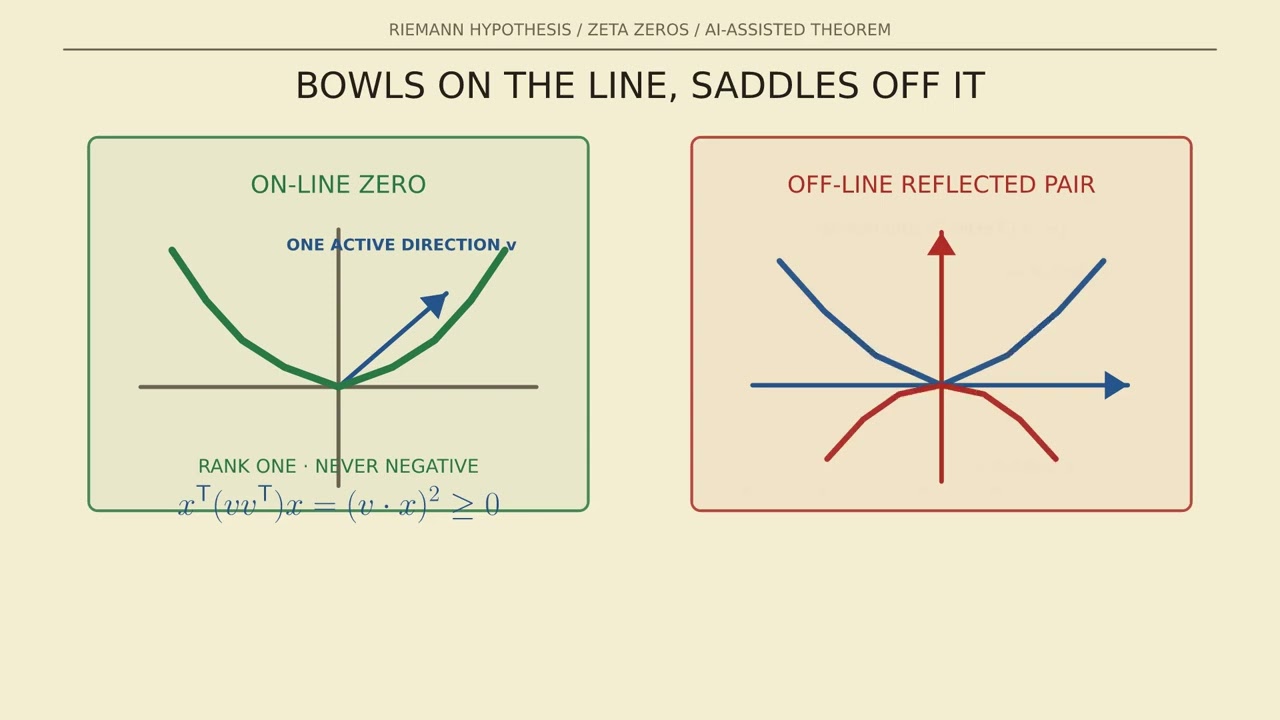
Instead of forcing term-wise positivity on the zero side, the proof maps Weil's explicit formula into a finite symmetric matrix and uses Sylvester's law of inertia to tightly balance the indefinite saddle contributions of off-line zeros. (13:10)
The core analytical lever is a rank–trace certificate derived from two elementary parabolas, which combines matrix trace, multiplicity budgets, and Frobenius norm estimates to yield the baseline 2/3 and 5/6 bounds. (15:24)
The mathematical proof was generated by Claude using a swarm of 60 sub-agents, independently verified by mathematicians Levent Alpoge and Ralph Furmani, and formalized in Lean 4 without unproven 'sorry' placeholders. (20:15)

Detailed notes

## Background Published on YouTube by channel Xiaol.x on August 21, 2026, this video addresses viral claims about artificial intelligence solving part of the Riemann Hypothesis by breaking down a major new AI-assisted preprint. The show notes clarify that while the Riemann Hypothesis itself remains open, the paper establishes a new unconditional density theorem proving that at least 67.25% of non-trivial zeta zeros are simple and lie on the critical line, utilizing finite matrix compression, inertia bookkeeping, and Lean 4 formal verification.

## TL;DR The presentation demystifies the distinction between proving the universal Riemann Hypothesis and establishing unconditional zero-density proportions. It details how historical attempts stalled because off-line zeros create indefinite quadratic forms where naive positivity fails, and shows how the new preprint circumvents this barrier by compressing the problem into finite real symmetric matrices. By treating on-line zeros as positive-definite bowls and off-line pairs as structured saddles, the proof applies Sylvester's law of inertia and an elementary rank–trace certificate to unconditionally guarantee that at least 2/3 (optimized to 67.25%) of zeros are simple and on the critical line, and at least 5/6 (optimized to 83.625%) are distinct. The video concludes by examining the multi-agent AI exploration workflow directed by human mathematicians, alongside the scope and practical realities of the project's Lean 4 formalization.

## Atmosphere & style The presentation strikes an engaging, intellectually rigorous, and lucid pedagogical tone that actively resists sensationalist AI hype in favor of clear mathematical mechanics. Using vivid visual metaphors—such as prime atoms, bilingual dictionaries, and bowls versus saddles—the narrator guides the audience through technical linear algebra with quiet confidence and clarity. The delivery blends serious academic exposition with candid, human moments—such as chuckling at the simplicity of high school parabolas or recounting how a Lean build filled up a local root partition—leaving viewers feeling empowered to verify the arithmetic for themselves.

## Bulletin - [07:49](https://www.youtube.com/watch?v=okGk7JdyM3w&t=469s) A new AI-assisted preprint unconditionally proves that at least 67.25% of non-trivial Riemann zeta zeros are simple and located on the critical line, with at least 83.625% being distinct. - [06:05](https://www.youtube.com/watch?v=okGk7JdyM3w&t=365s) The result significantly surpasses the previous unconditional record of approximately 40.7511% established in 2020 by Pratt, Robles, Zaharescu, and Zeindler. - [13:10](https://www.youtube.com/watch?v=okGk7JdyM3w&t=790s) Instead of forcing term-wise positivity on the zero side, the proof maps Weil's explicit formula into a finite symmetric matrix and uses Sylvester's law of inertia to tightly balance the indefinite saddle contributions of off-line zeros. - [15:24](https://www.youtube.com/watch?v=okGk7JdyM3w&t=924s) The core analytical lever is a rank–trace certificate derived from two elementary parabolas, which combines matrix trace, multiplicity budgets, and Frobenius norm estimates to yield the baseline 2/3 and 5/6 bounds. - [20:15](https://www.youtube.com/watch?v=okGk7JdyM3w&t=1215s) The mathematical proof was generated by Claude using a swarm of 60 sub-agents, independently verified by mathematicians Levent Alpoge and Ralph Furmani, and formalized in Lean 4 without unproven 'sorry' placeholders.

## Key takeaways - [00:00](https://www.youtube.com/watch?v=okGk7JdyM3w&t=0s) Bernhard Riemann discovered that the non-trivial zeros of the zeta function act as harmonic correction waves controlling the error oscillations when counting prime numbers. - [02:53](https://www.youtube.com/watch?v=okGk7JdyM3w&t=173s) The Riemann Hypothesis posits that every single non-trivial zero lies exactly on the critical line Re(s) = 1/2, a symmetry line dictated by the functional equation. - [06:05](https://www.youtube.com/watch?v=okGk7JdyM3w&t=365s) Proving that a certain fraction of zeros lie on the critical line provides a population density guarantee, not a proof of the Riemann Hypothesis, as a single off-line zero would disprove RH. - [07:49](https://www.youtube.com/watch?v=okGk7JdyM3w&t=469s) The new theorem unconditionally proves that at least (2/3 - o(1)) of non-trivial zeros are simple and on the line, and at least (5/6 - o(1)) are distinct as T tends to infinity. - [09:17](https://www.youtube.com/watch?v=okGk7JdyM3w&t=557s) Hugh Montgomery established a conditional 2/3 simplicity fraction in 1973 under RH, but prior unconditional proofs failed because off-line zeros create indefinite quadratic forms that break term-wise positivity. - [10:51](https://www.youtube.com/watch?v=okGk7JdyM3w&t=651s) Evaluating pairs of shifted test windows through Weil's explicit formula compresses the infinite-dimensional problem into a computable, finite real symmetric matrix G. - [12:17](https://www.youtube.com/watch?v=okGk7JdyM3w&t=737s) Zeros on the critical line contribute positive semi-definite rank-1 'bowls' (v v^T) to the matrix, whereas off-line pairs produce indefinite 'saddles' (2(a a^T - b b^T)). - [13:10](https://www.youtube.com/watch?v=okGk7JdyM3w&t=790s) Sylvester's law of inertia proves that an off-line saddle can contribute at most one uphill positive direction, enabling an exact balance sheet of negative directions rather than requiring universal positivity. - [13:54](https://www.youtube.com/watch?v=okGk7JdyM3w&t=834s) The proof evaluates four matrix metrics on G: rank (active dimensions), positive inertia (uphill count), trace (total signed mass asymptotic to N), and Frobenius norm squared (spectral crowding asymptotic to 4/3 N). - [15:24](https://www.youtube.com/watch?v=okGk7JdyM3w&t=924s) The rank–trace certificate is derived from the scalar identities (x - 1)^2 >= 0 and (x - 2)^2 >= 0 together with the von Neumann trace inequality. - [16:58](https://www.youtube.com/watch?v=okGk7JdyM3w&t=1018s) Combining the rank–trace certificate with the total multiplicity budget (<= N) cancels intermediate variables to establish the baseline simple on-line bound 4 - 2 - 4/3 = 2/3. - [18:44](https://www.youtube.com/watch?v=okGk7JdyM3w&t=1124s) Replacing a flat test window with an optimized Montgomery–Taylor cosine window reduces spectral leakage, lowering the Frobenius parameter from 4/3 to 1.32750 to achieve the 67.25% and 83.625% records. - [18:44](https://www.youtube.com/watch?v=okGk7JdyM3w&t=1124s) The second-moment method at Fourier bandwidth 1 possesses an intrinsic theoretical ceiling near 0.6818, which is an artifact of the method rather than a property of zeta zeros. - [20:15](https://www.youtube.com/watch?v=okGk7JdyM3w&t=1215s) Claude authored the core mathematical argument through guided search across 60 sub-agents and 650 dead ends, while mathematicians Alpoge and Furmani validated the reasoning and assumed formal scholarly responsibility. - [21:46](https://www.youtube.com/watch?v=okGk7JdyM3w&t=1306s) A companion Lean 4 formalization confirms the logical validity of the density theorems from Lean's standard foundational axioms, though traditional peer review of the preprint remains ongoing.

## Detailed walkthrough ### [00:00](https://www.youtube.com/watch?v=okGk7JdyM3w&t=0s) What Problem Are We Trying to Solve?

The journey begins with the fundamental building blocks of arithmetic: the positive integers. Prime numbers—such as 2, 3, 5, 7, and 11—cannot be factored into smaller positive pieces. They act as the indivisible "atoms" from which every single integer is constructed via multiplication. Yet, when laid out along the number line, their exact positions appear erratic and unpredictable. Bernhard Riemann's revolutionary insight was to avoid guessing the next prime directly; instead, he analyzed a single mathematical machine—the Riemann zeta function—that encodes all prime numbers simultaneously.

Like any mathematical function, zeta takes an input and produces an output. Of supreme interest are the specific complex inputs that cause the output to vanish entirely—the zeros of the function. While some zeros are straightforward, the vast majority of mysterious non-trivial zeros reside in a vertical strip of the complex plane known as the critical strip, centered on a symmetry axis called the critical line. The Riemann Hypothesis (RH) is a single, uncompromising universal statement: every single non-trivial zero lies exactly on this central line. "Every means no exceptions," extending even to zeros infinitely high up the strip that no supercomputer could ever numerically verify.

Understanding these zero locations is vital because Riemann's explicit formula transforms them into harmonic correction waves that dictate the precise error when approximating the count of primes.

```mermaid flowchart TD accTitle: The Prime to Zero Translation Pipeline accDescr: A pipeline showing how integers factor into primes, enter the zeta function, produce zeros, and govern prime-counting errors. subgraph Arithmetic["Arithmetic Foundation"] A["Positive Integers"] -->|"Unique Factorization"| B["Prime Atoms (2, 3, 5, 7...)"] end subgraph Analysis["Analytic Machinery"] B -->|"Euler Product & Sum"| C["Riemann Zeta Function ζ(s)"] C -->|"Vanishing Points"| D["Non-Trivial Zeros (ρ = β + iγ)"] end subgraph ErrorControl["Prime Distribution"] D -->|"Explicit Formula Oscillations"| E["Correction Waves (x^ρ / ρ)"] E -->|"Controls Fluctuations"| F["Prime-Counting Error"] end ```

- **The Road Map**: Positive integers decompose into prime atoms; primes enter the zeta function; zeta produces non-trivial zeros; the locations of those zeros govern the error bounds in prime-counting estimates.

---

[01:33](https://www.youtube.com/watch?v=okGk7JdyM3w&t=93s) One Function Speaks Integers and Primes: The Bilingual Dictionary

To see how one function bridges two entirely different mathematical worlds, consider Leonhard Euler's discovery. For any complex number $s$ whose real part is strictly greater than 1, the zeta function can be defined as the infinite series: $$\zeta(s) = \sum_{n=1}^{\infty} \frac{1}{n^s}$$ Simultaneously, Euler proved that this identical quantity equals an infinite product taken over all prime numbers $p$: $$\zeta(s) = \prod_{p} \left(1 - p^{-s}\right)^{-1}$$

The infinite sum speaks the language of all integers, whereas the infinite product speaks the language of prime atoms. The fundamental theorem of arithmetic—unique prime factorization—is what guarantees that these two expressions are identical. When expanding each geometric factor $(1 - p^{-s})^{-1} = 1 + p^{-s} + p^{-2s} + \dots$ across all primes, one selects zero, one, two, or more copies of each prime factor, assembling every single positive integer exactly once.

This dual formulation serves as a "bilingual dictionary." If one can master its complex analytic grammar—specifically the precise inputs where the function evaluates to zero—one can translate smooth, global facts about a complex analytic function directly back into sharp, concrete truths about the jagged, irregular distribution of the prime numbers.

---

[02:53](https://www.youtube.com/watch?v=okGk7JdyM3w&t=173s) The Complex Map and Its Critical Line Symmetry

Visualizing the zeta function requires treating the input $s = \sigma + it$ as a coordinate on a two-dimensional map, where $\sigma$ is the horizontal coordinate (the real part) and $t$ is the vertical coordinate (the imaginary part). To the right of the vertical line $\sigma = 1$, Euler's prime product converges unconditionally and none of its individual factors equal zero, ensuring that the zeta function has no zeros anywhere in that half-plane.

Using analytic continuation, the domain of zeta extends across the entire complex plane, punctuated by only a single simple pole at $s = 1$. The functional equation establishes an exact reflection relating the function's value at $s$ to its value at $1 - s$: - **Trivial zeros**: The reflection produces predictable, well-understood zeros at the negative even integers ($-2, -4, -6, \dots$). - **The critical strip**: Once the trivial zeros are set aside, all remaining non-trivial zeros are trapped entirely within the vertical band $0 \le \sigma \le 1$. - **The symmetry axis**: If $\rho = \beta + i\gamma$ is a non-trivial zero, the functional equation forces $1 - \beta + i\gamma$ to be a zero, while complex conjugation forces $\beta - i\gamma$ to be a zero. Setting the horizontal reflection equal to itself ($\beta = 1 - \beta$) yields $2\beta = 1$, which forces $\beta = 1/2$.

The critical line $\text{Re}(s) = 1/2$ is therefore no arbitrary aesthetic choice—it is the geometric axis of symmetry demanded by the functional equation. The Riemann Hypothesis asserts that every non-trivial zero is pinned horizontally to this line. A single zero departing from $\beta = 1/2$ anywhere in the infinite strip would immediately disprove the hypothesis.

---

[04:38](https://www.youtube.com/watch?v=okGk7JdyM3w&t=278s) How Zeros Control Prime-Counting Errors

Counting the number of primes up to a given bound $x$ produces an irregular staircase function: it stays completely flat between primes, then abruptly jumps upward by 1 at every prime. A smooth logarithmic integral curve tracks the broad upward climb of the staircase, but it fails to capture the intricate, jagged oscillations along the way. Riemann's explicit formula proves that these fluctuations are assembled from an infinite superposition of waves, each indexed by a non-trivial zero $\rho$.

In schematic form, each zero $\rho = \beta + i\gamma$ contributes an oscillatory term proportional to: $$\frac{x^\rho}{\rho} = \frac{x^\beta \cdot x^{i\gamma}}{\rho} = \frac{x^\beta e^{i\gamma \log x}}{\rho}$$ The imaginary coordinate $\gamma$ dictates the frequency of the wave (how rapidly it wiggles as $x$ increases), while the real coordinate $\beta$ acts as an amplitude exponent dictating how large the fluctuation can grow. If every non-trivial zero has $\beta = 1/2$, every correction wave shares the exact same square-root growth scale ($x^{1/2}$). An off-line zero with $\beta > 1/2$ would produce a much larger, destabilizing surge. Thus, the critical line serves as the proposed universal balance law governing the error in counting primes.

---

[06:05](https://www.youtube.com/watch?v=okGk7JdyM3w&t=365s) Counting Zeros: What Does a Percentage Guarantee Mean?

To measure progress toward understanding the critical line, mathematicians track zero counts within bounded windows. Consider a toy window containing four zero locations where one location happens to be a double root: - Counted with multiplicity ($N$), that double root counts as 2, yielding a total of $N = 5$. - Counted as distinct locations ($N_d$), the double root counts once, yielding $N_d = 4$. - A zero is termed simple if its multiplicity is strictly equal to 1. - The quantity $N_0^s$ counts only zeros that are both simple and located strictly on the critical line.

A lower bound on $N_0^s$ guarantees both precise geometric location ($\beta = 1/2$) and non-repetition (multiplicity 1) simultaneously. However, this is strictly a statistical "population guarantee," not a partial proof of the universal hypothesis. Even proving that $99.999\%$ of zeros are simple and on the line would still leave the Riemann Hypothesis unproven if rare exceptions persisted at higher altitudes.

Furthermore, asymptotic statements phrased as $2/3 - o(1)$ mean that for any positive tolerance $\varepsilon > 0$, the guaranteed fraction exceeds $2/3 - \varepsilon$ once the height $T$ is sufficiently large; it does not promise an exact $2/3$ proportion inside every small finite interval.

- **Historical benchmarks**: In 2020, Kyle Pratt, Nicolas Robles, Alexandru Zaharescu, and Dirk Zeindler proved unconditionally that at least approximately $41.7293\%$ of non-trivial zeros lie on the critical line, and at least $40.7511\%$ are simple and on the line. - While recent preprints occasionally cite $5/12$ ($\approx 41.67\%$) as the informal benchmark for simple zeros, the actual prior unconditional record stood at $40.7511\%$.

---

[07:49](https://www.youtube.com/watch?v=okGk7JdyM3w&t=469s) The Exact Breakthrough: Unconditional Bounds

Let $N(T, 2T)$ count the total number of non-trivial zeros whose vertical heights lie between $T$ and $2T$, counting multiplicities. The breakthrough paper establishes that, as $T \to \infty$: $$N_0^s \ge \left(\frac{2}{3} - o(1)\right) N(T, 2T)$$ Within that same height interval, the number of distinct zeros $N_d$ satisfies: $$N_d \ge \left(\frac{5}{6} - o(1)\right) N(T, 2T)$$

Crucially, this mathematical proof is entirely unconditional. It requires no assumption of the Riemann Hypothesis, no hypothetical zero-density conjectures, and no premise restricting zeros to an artificially narrow box around the critical line.

When the simplest flat measuring window is upgraded to the optimized Montgomery-Taylor window, the resulting numerical constants improve noticeably: - The proportion of zeros certified to be **simple and on the critical line** reaches at least **$0.67250$** (or $67.25\%$). - The proportion of **distinct zeros** reaches at least **$0.83625$** (or $83.625\%$).

The theorem also holds in cumulative form across the interval from height $0$ to $T$, and extends to every fixed primitive Dirichlet $L$-function. However, logical clarity must be maintained: a certified lower bound of $67.25\%$ means that at least that much good behavior is mathematically forced. It places no upper ceiling on the true fraction, nor does it imply that the remaining $32.75\%$ of zeros lie off the line.

---

[09:17](https://www.youtube.com/watch?v=okGk7JdyM3w&t=557s) The Old Approach, Narrow Boxes, and the Missing Bridge

The path to this result represents the culmination of a decades-long mathematical relay race: - **Hugh Montgomery (1973)**: Applied pair-correlation statistics—analyzing differences between pairs of zero heights—to deduce a $2/3$ simplicity proportion, but his derivation was strictly conditional on the Riemann Hypothesis. - **Farzad Aryan**: Uncovered an unconditional second-moment estimate on the prime side. - **Baluyot, Goldston, Suriajaya, and Turnage-Butterbaugh**: Formulated an unconditional version of Montgomery's theorem evaluated across all complex zeros. - **Goldston, Suriajaya, and collaborators**: Demonstrated that the benchmarks of $2/3$ and $5/6$ would follow naturally if one could merely prove that zeros stayed confined within an exceedingly narrow vertical box hugging the critical line.

These earlier investigations isolated the exact technical barrier—the "missing bridge." Under the assumption of RH, every zero ordinate $\gamma$ is real, which causes the zero-side expression to behave as a sum of non-negative squares; under those conditions, throwing away unwanted terms to establish an inequality is completely legal. Without RH, however, an off-line zero exhibits a complex ordinate whose reflected partner introduces negative directions. The resulting quadratic form becomes indefinite, making the algebraic instruction to simply "drop the remaining terms" mathematically invalid.

While the statistical machinery on the prime side was already robust, unconditional proofs repeatedly hit a "death point" on zero-side positivity. The breakthrough does not attempt to repair or force positivity where none exists—it abandons the need for positivity altogether.

---

[10:51](https://www.youtube.com/watch?v=okGk7JdyM3w&t=651s) Compressing an Infinite Problem into a Matrix

André Weil's explicit formula synthesizes prime data and zero data into an infinite-dimensional Hermitian form, denoted $W$. A Hermitian form acts as a mathematical apparatus that ingests a test signal and returns a real-valued quadratic measurement, analogous to physical energy. Remarkably, proving that Weil's full form remains positive semi-definite for every valid test function is mathematically equivalent to proving the Riemann Hypothesis itself.

Rather than tackling the infinite-dimensional form directly, the new approach executes a computable compression: 1. It selects numerous shifted copies of a localized test window, spaced uniformly throughout the height interval $[T, 2T]$. 2. Every pair of test windows is evaluated through Weil's form $W$. 3. These pairwise measurements form the entries of a finite, real symmetric matrix $G$, whose dimension is roughly comparable to the total zero count $N(T, 2T)$ in that interval.

The explicit formula enables matrix $G$ to be read in two complementary languages:

| Zero-Side Representation | Prime-Side Representation | |:--- |:--- | | Decomposes into structured geometric blocks directly contributed by individual zeros and pairs of zeros. | Evaluates the global trace and the squared Frobenius norm using classical mean-value estimates. |

The compression functions like recording an orchestra through an array of carefully placed microphones: while individual acoustic nuances are omitted, essential collective statistical properties are preserved. The proof succeeds at the exact junction where the zero-side matrix geometry meets the prime-side mean-value calculations.

---

[12:17](https://www.youtube.com/watch?v=okGk7JdyM3w&t=737s) Bowls on the Line and Saddles Off It

Examining the zero-side decomposition of the matrix $G$ reveals the geometric signatures left by different zeros. Each zero produces a response vector $v$ across the bank of test windows: - **Zeros on the critical line**: If a zero resides on $\text{Re}(s) = 1/2$, its response vector $v$ is purely real. Its contribution to the matrix is the outer product $v v^T$. When tested against any arbitrary vector $x$, the quadratic form evaluates to $x^T (v v^T) x = (v \cdot x)^2 \ge 0$. Geometrically, this represents a rank-1 positive semi-definite "bowl"—curving upward along a single direction and remaining entirely flat across all perpendicular dimensions. - **Off-line zeros**: An off-line zero inevitably arrives paired with its functional-equation reflection. Writing its complex response vector as $a + ib$, the combined contribution of the reflected pair cancels the imaginary cross-terms, leaving the real symmetric form: $$2\left(a a^T - b b^T\right)$$ Because this expression contains a positive term ($a a^T$) alongside an explicitly negative term ($-b b^T$), an off-line zero generates an indefinite saddle geometry rather than a bowl, perfectly encapsulating the indefinite nature that previously derailed unconditional proofs.

[13:10](https://www.youtube.com/watch?v=okGk7JdyM3w&t=790s) Saddles Off the Line and Sylvester's Law of Inertia

Testing an off-line block along one vector yields an uphill climb, while testing it along another sends you downhill. Geometrically, that is a saddle: an operator possessing at most one positive and one negative direction. In earlier analytical attempts, this structural minus sign was viewed purely as an obstruction that ruined term-wise positivity. When researchers demanded that every term in an expansion stay strictly positive, a single negative eigenvalue destroyed the entire machine.

The breakthrough insight was realizing that this damage is not chaotic—it is strictly bounded and structured. Any reflected off-line pair of zeros can inject exactly one uphill direction into the system. Under Sylvester's law of inertia, no invertible change of coordinates can disguise, inflate, or destroy that fundamental count of positive and negative directions. Rather than mourning the death of universal positivity, one can simply keep an exact balance sheet of the negative directions.

[13:54](https://www.youtube.com/watch?v=okGk7JdyM3w&t=834s) The Four Matrix Measurements: Rank, Inertia, Trace, and Frobenius Norm

To turn this geometric intuition into hard arithmetic, the argument relies on four foundational concepts from matrix analysis. Any real symmetric matrix possesses mutually orthogonal eigendirections, each exerting a signed scaling factor known as an eigenvalue. Translating infinite-dimensional spectral behavior into a manageable ledger requires four specific summary statistics:

```mermaid flowchart TD accTitle: Four Matrix Statistics accDescr: Diagram illustrating how eigenvalues are aggregated into Rank, Positive Inertia, Trace, and Frobenius Norm Squared. subgraph Counts ["Direction Counts"] direction1["All Non-Zero Directions"] --> Rank["Rank<br/>(Activity)"] direction2["Uphill Directions (> 0)"] --> Inertia["Positive Inertia<br/>(Uphill Count)"] end subgraph MassAndSpread ["Mass and Spread"] eigenvalues["Eigenvalues with Signs"] --> Trace["Trace<br/>(Total Signed Mass)"] squared["Squared Eigenvalues"] --> Frob["Frobenius Norm Squared<br/>(Spectral Crowding)"] end ```

- **Rank:** Counts the total number of non-zero eigenvalues, revealing how many directions in the space are actively engaged. - **Positive Inertia:** Tallies strictly positive eigenvalues, counting how many directions point strictly uphill. - **Trace:** Sums all eigenvalues while preserving their signs, giving the total signed mass of the system. - **Frobenius Norm Squared:** Sums the squares of the eigenvalues. Because squaring erases signs and penalizes heavy concentration, this metric acts as a penalty against spectral crowding.

A helpful toy example is a four-dimensional matrix with eigenvalues $2, 1, -1,$ and $0$. Its rank is $3$ (three active directions), its positive inertia is $2$ (two uphill slopes), its trace is $2 + 1 - 1 + 0 = 2$, and its squared Frobenius norm is $2^2 + 1^2 + (-1)^2 + 0^2 = 6$.

When this machinery is applied to the compressed zeta matrix $G$, prime-number estimates yield two concrete receipts: - The trace $\operatorname{Tr}(G)$ is asymptotic to $N$, representing exactly one unit of mass per zero counted with multiplicity. - For a simple flat test window, the Frobenius norm squared $\|G\|_F^2$ is asymptotic to $\frac{4}{3}N$.

Although these two global totals do not disclose the individual eigenvalues, their interaction with the bowl-and-saddle block structure mathematically forces a strict minimum of simple, on-line rank.

[15:24](https://www.youtube.com/watch?v=okGk7JdyM3w&t=924s) Deriving the Rank–Trace Certificate from School Parabolas

To pin down that minimum rank, the matrix is split into two components: a positive semi-definite matrix $P$ constructed from the well-behaved, simple on-line zeros (having rank at most $R$), and a remainder matrix $Q$ holding all other zero contributions, which contributes at most $B$ positive directions. $Q$ is further decomposed into its positive and negative spectral components, $Q = Q_+ - Q_-$.

Remarkably, the heavy analytical lifting rests on two elementary high school identities: $(x - 1)^2 \ge 0 \implies x^2 \ge 2x - 1$ and $(x - 2)^2 \ge 0 \implies x^2 \ge 4x - 4$. The first parabola charges at most one unit of penalty for every active direction of $P$ when juxtaposed against the negative spectrum of $Q$. The second parabola assesses a cost of at most four units for each of the $B$ positive directions hidden inside $Q$. Applying the von Neumann trace inequality aligns the worst possible eigenvalue pairings, and combining the scalar bounds yields the master certificate:

$$R \ge 2\operatorname{Tr}(P) + 4\operatorname{Tr}(Q) - 4B - \|P + Q\|_F^2$$

"Nothing mystical entered," the speaker observes. The coefficients $1$, $2$, and $4$ are merely the centers and quadratic costs of two ordinary algebraic parabolas. The actual stroke of creative genius was recognizing that this elementary certificate mirrors the exact block accounting generated by Riemann zeta zeros.

[16:58](https://www.youtube.com/watch?v=okGk7JdyM3w&t=1018s) Deriving the 2/3 Simple and 5/6 Distinct Zero Bounds

Once the general certificate is established, the specific zero classifications can be fed into the formula: - Let $P_1$ contain only simple zeros lying on the critical line, with $S_1$ counting their total. - Let $S_2$ count multiple zero locations on the line. - Let $P$ count the off-line reflected pairs.

The remainder matrix $Q'$ has at most $S_2 + P$ positive directions. Crucially, the total multiplicity budget cannot exceed $N$:

$$\operatorname{Tr}(P_1) + 2(S_2 + P) \le N$$

A simple zero consumes a single unit of multiplicity, whereas any multiple zero or off-line pair costs at least two units. Substituting this budget constraint into the rank–trace certificate causes the clutter to collapse into a streamlined lower bound on the simple on-line rank:

$$\operatorname{rank}(P_1) \ge 4\operatorname{Tr}(G) - 2N - \|G\|_F^2$$

From prime-side estimates, $\operatorname{Tr}(G) = N + o(N)$, and under a flat test window, $\|G\|_F^2 = \frac{4}{3}N + o(N)$. Evaluating the scalar coefficients gives:

$$4 - 2 - \frac{4}{3} = \frac{2}{3}$$

Because each rank-one piece originates from a distinct simple on-line zero, at least $\frac{2}{3}$ (or $66.67\%$) of all zeros must be simple and lie on the critical line.

```mermaid flowchart LR accTitle: Budget Allocation to Simple and Distinct Bounds accDescr: Flow diagram showing how the multiplicity budget and matrix traces combine to prove the 2/3 simple and 5/6 distinct zero thresholds. subgraph Budget ["Budget Inputs"] Tr["Trace Mass: 4N"] Mult["Multiplicity Cap: -2N"] Frob["Flat Window Spread: -(4/3)N"] end subgraph Outputs ["Final Proportions"] Simple["Simple & On-Line: >= 2/3 N (66.67%)"] Distinct["Distinct Zeros: >= 5/6 N (83.33%)"] end Tr & Mult & Frob --> Simple Simple -->|"Algebraic Recombination"| Distinct ```

Rearranging that identical certificate to account for distinct zeros produces $3S_1 + 4(S_2 + P) \ge \frac{8}{3}N$. Subtracting the multiplicity budget $S_1 + 2(S_2 + P) \le N$ leaves $2(S_1 + S_2 + P) \ge \frac{5}{3}N$. Dividing across by two proves that at least $\frac{5}{6}$ (or $83.33\%$) of all non-trivial zeros are distinct.

[18:44](https://www.youtube.com/watch?v=okGk7JdyM3w&t=1124s) The Optimized 67.25% Bound and the Spectral Ceiling

The clean fraction $\frac{2}{3}$ is tied directly to the flat test window, which fixes the normalized squared size parameter $R$ at $\frac{4}{3}$. In general, the rank–trace certificate establishes that: - The simple on-line proportion is at least $2 - R$. - The distinct proportion is at least $\frac{1}{2}(3 - R)$.

A flat window acts like a hard-edged stencil, leaking spectral energy and inflating $R$. Replacing it with a smoother, optimized Montgomery–Taylor cosine window reduces the spectral leakage, driving $R$ down to approximately $1.32750$.

Substituting this tighter value into the certificates yields the headline records: - **Simple and on the critical line:** at least $2 - 1.32750 = 0.67250$, or **$67.25\%$**. - **Distinct zeros:** at least $\frac{1}{2}(3 - 1.32750) = 0.83625$, or **$83.625\%$**.

Within the classical family of test windows, this choice is optimal. The preprint also investigates a broader theoretical class of certificates restricted to first and second moments at Fourier bandwidth 1, uncovering a mathematical ceiling near $0.6818$. This ceiling is an inherent barrier of the second-moment method, not a limit on the Riemann Hypothesis itself.

Importantly, the numerical enclosure certificate for this $0.6818$ ceiling sits outside the Lean formalization kernel—a known gap documented openly in the project's public issue tracker. None of the core unconditional theorems ($\frac{2}{3}$, $67.25\%$, $\frac{5}{6}$, or $83.625\%$) rely on that external ceiling calculation.

[20:15](https://www.youtube.com/watch?v=okGk7JdyM3w&t=1215s) Behind the AI Workflow: Sub-Agents, Tokens, and Authorship

According to Anthropic's research report, the project was directed and framed by human researchers who guided the automated search. The exploration engine deployed a swarm of roughly 60 sub-agents, generating approximately 31 million output tokens, executing around 2,400 shell commands, and authoring hundreds of auxiliary Python scripts.

The progression was far from an effortless one-shot prompt: - The initial exploration accumulated roughly 650 dead ends and failed concepts. - In a subsequent deep session, the system found a weaker route based on positive inertia, invited adversarial counter-checks, and eventually surfaced the scalar rank–trace lever that unlocks the $\frac{2}{3}$ threshold. - While curated transcripts corroborate this narrative arc, they remain selected records rather than an exhaustive audit log of every background computation, and the exact research model version remains proprietary.

Authorship and scholarly credit require careful framing. The arXiv preprint lists mathematicians Levent Alpoge and Ralph Furmani. The paper's source notes state that Claude discovered and authored the mathematical argument, while Alpoge and Furmani examined it, independently validated each step, contextualized the findings within the analytic number theory literature, communicated the manuscript, and accepted formal responsibility for any remaining errors. This represents a modern paradigm of human-steered machine exploration paired with rigorous human mathematical accountability—not an autonomous chatbot rubber-stamping its own discoveries.

[21:46](https://www.youtube.com/watch?v=okGk7JdyM3w&t=1306s) The Lean 4 Formalization: What It Verifies and What It Doesn't

To anchor the paper's mathematical integrity, the authors provided an extensive formalization in Lean 4. An inspection of the repository reveals: - The primary theorem files and analytical proofs contain zero `sorry` placeholders. - An axiom audit confirms reliance solely on Lean's standard foundational logical axioms. - Dedicated comparator files restate the main claims directly against Mathlib types so external Lean kernels can verify that the proven targets match established mathematical definitions. - The project formalizes reusable matrix theory, upstreaming formal proofs for Sylvester's law of inertia and the von Neumann trace inequality.

Yet formal verification must not be conflated with universal truth. Lean rigorously verifies that deductions follow logically from coded definitions and imported premises; it cannot manufacture instant academic consensus around a brand-new preprint, endorse corporate publicity claims, or bypass traditional peer review.

The narrator notes that a source review revealed no issues alleging mathematical flaws in the core density theorems. One tracker item simply clarified the wording of an equality case without disturbing the inequality, while another involved the external ceiling certificate. On a personal note, the narrator mentions being unable to finish a local build because installing the pinned Lean toolchain filled up their root partition—underscoring that a verified repository requires substantial infrastructure to compile. The responsible takeaway: this is a major, extraordinarily well-formalized preprint backed by deep human checking, published while conventional peer review is just getting underway.

[23:21](https://www.youtube.com/watch?v=okGk7JdyM3w&t=1401s) The Translation Game: From Prime Atoms to Critical Zeros

To tie the entire journey together, the visual lesson reframes the breakthrough as an elegant, multi-stage game of mathematical translation:

```mermaid flowchart TD accTitle: The Complete Translation Game accDescr: Pipeline showing primes turning into explicit formulas, waves, finite matrices, eigenvalues, and finally zeros on the critical line. Primes["Prime Atoms"] -->|"Explicit Formula"| Waves["Zero Waves"] Waves -->|"Test Window Sampling"| Matrix["Finite Matrix G"] Matrix --> Geometries["Bowls (On-Line) vs. Saddles (Off-Line)"] Geometries --> Stats["Global Stats: Trace (N) & Frobenius (4/3 N)"] Stats -->|"Rank-Trace Inequality"| InertiaCount["Forced Good Eigendirections"] InertiaCount --> Result["At Least 67.25% Simple Zeros on Re(s) = 1/2"] ```

The arithmetic can now be replayed in a single line:

$$4N \text{ (from trace)} - 2N \text{ (from the counting budget)} - \frac{4}{3}N \text{ (from spectral crowding)} = \frac{2}{3}N$$

The video closes with a snort of amusement and an invitation for viewers to actively play with the mathematical machinery rather than merely admiring the headlines: - Draw a doubled zero and calculate its multiplicity under three separate counting conventions. - Construct a toy matrix with four arbitrary eigenvalues and compute its rank, positive inertia, trace, and squared Frobenius norm by hand. - Explain to a friend why an off-line saddle destroys naive, term-wise positivity, yet remains completely powerless against inertia bookkeeping.

Mastering those three exercises transforms a viral AI claim into solid mathematical ground that any student or researcher can independently inspect, question, and rebuild.

## Notable quotes > [00:00](https://www.youtube.com/watch?v=okGk7JdyM3w&t=0s) Every means no exceptions

> [15:24](https://www.youtube.com/watch?v=okGk7JdyM3w&t=924s) Nothing mystical entered

> Did AI solve 67% of the Riemann Hypothesis? No—the Riemann Hypothesis remains open.

> The key distinction: RH says every nontrivial zero lies on the critical line. A density theorem classifies a guaranteed fraction. Even 99.999% would not prove RH if rare exceptions remained.

> Its central innovation replaces a failed positivity argument with finite-dimensional inertia bookkeeping.

> The preprint is very new, and conventional expert review is still ongoing.

> [21:46](https://www.youtube.com/watch?v=okGk7JdyM3w&t=1306s) What Lean verification does—and does not—prove

> [23:21](https://www.youtube.com/watch?v=okGk7JdyM3w&t=1401s) The complete mathematical translation game

## Mentioned Alexandru Zaharescu, André Weil, Anthropic, Bernhard Riemann, Claude, Clay Mathematics Institute, Dirk Zeindler, Farzad Aryan, Hugh Montgomery, Kyle Pratt, Lean 4, Leonhard Euler, Levent Alpoge, Mathlib, Montgomery-Taylor window, Nicolas Robles, Python, Ralph Furmani, Riemann Hypothesis, Sylvester's law of inertia, von Neumann trace inequality

## Video description Did AI solve 67% of the Riemann Hypothesis? No—the Riemann Hypothesis remains open. But a remarkable new AI-assisted preprint proves a major unconditional result about the zeros of the Riemann zeta function.

Starting from the fundamentals, this visual lesson explains:

- What the Riemann Hypothesis actually asks - How primes are encoded by the zeta function - What zeta zeros are and why the critical line is (\Re(s)=1/2) - Why 67.25% does not mean “67% of RH is solved” - How the new theorem guarantees at least 67.25% of zeros are simple and on the critical line - Why at least 83.625% are distinct - How finite matrices, eigenvalues, inertia, and a rank–trace inequality produce these bounds - What Claude contributed, what humans verified, and what the Lean 4 formalization checks

The key distinction: RH says every nontrivial zero lies on the critical line. A density theorem classifies a guaranteed fraction. Even 99.999% would not prove RH if rare exceptions remained.

The work substantially improves the previous unconditional simple-on-line record of approximately 40.7511%. Its central innovation replaces a failed positivity argument with finite-dimensional inertia bookkeeping. The preprint is very new, and conventional expert review is still ongoing.

Chapters

00:00 What problem are we solving? 01:33 One function speaks integers and primes 02:53 The complex map and its critical line 04:38 How zeros control prime-counting errors 06:05 What does “67% of the zeros” mean? 07:49 The exact breakthrough 09:17 The old approach and its missing bridge 10:51 Compressing an infinite problem into a matrix 12:17 Bowls on the line, saddles off it 13:53 Rank, inertia, trace, and Frobenius norm 15:24 Deriving the rank–trace certificate 16:58 Where two thirds and five sixths come from 18:44 Why the optimized bound is 67.25% 20:15 What the AI research process did 21:46 What Lean verification does—and does not—prove 23:21 The complete mathematical translation game

Primary Sources

Paper: https://arxiv.org/abs/2608.13637 Anthropic research report: https://www.anthropic.com/research/riemann-zeta Lean 4 formalization: https://github.com/anthropics/zeta-23-lean Clay Mathematics Institute overview: https://www.claymath.org/wp-content/uploads/2022/05/riemann.pdf Riemann’s 1859 memoir: https://www.maths.tcd.ie/pub/HistMath/People/Riemann/Zeta/EZeta.pdf Previous unconditional record: https://arxiv.org/abs/1802.10521

#RiemannHypothesis #Mathematics #ArtificialIntelligence #ClaudeAI #Lean4

[Source](https://www.youtube.com/watch?v=okGk7JdyM3w)

中文简报

Anthropic AI助力证明黎曼zeta函数零点达创纪录的67%界限这项无条件的67.25%密度证明通过有限矩阵惯性记账法绕过了停滞不前的正定性方法，但由于统计保证无法排除孤立的临界线外异常点，黎曼猜想仍未得到彻底证明。该演讲阐明了证明普适黎曼猜想与建立无条件零点密度比例之间的区别。它详细阐述了以往尝试如何因临界线外的零点导致简单正定性失效的不定二次型而陷入停滞，并展示了最新预印本如何通过将问题压缩至有限实对称矩阵来规避这一障碍。通过将临界线上的零点视为正定碗状结构，并将临界线外的成对零点视为结构化马鞍面，该证明应用了西尔维斯特惯性定律和基于初等秩-迹证书，无条件保证了至少2/3（优化至67.25%）的零点为单零点且位于临界线上，以及至少5/6（优化至83.625%）为互异零点。视频最后探讨了由人类数学家指导的多智能体AI探索工作流，以及该项目在Lean 4形式化验证中的范畴与现实实践。一项最新AI辅助的预印本无条件证明了黎曼zeta函数的非平凡零点中，至少有67.25%是位于临界线上的单零点，且至少有83.625%是互异零点。 (7:49) 该结果显著超越了Pratt、Robles、Zaharescu和Zeindler在2020年创下的约40.7511%的先前无条件纪录。 (6:05) 该证明并未在零点侧强行要求逐项正定，而是将韦伊显式公式映射至有限对称矩阵，并利用西尔维斯特惯性定律严密平衡了临界线外零点的不定马鞍面贡献。 (13:10) 核心分析手段是源自两个初等抛物线的秩-迹证书，该证书结合了矩阵迹、重数预算和Frobenius范数估计，得出了2/3和5/6的基准界限。 (15:24) 该数学证明由Claude借助由60个子智能体组成的群体生成，并由数学家Levent Alpoge和Ralph Furmani独立验证，同时在Lean 4中完成了形式化，不含未证明的“sorry”占位符。 (20:15)

Reading summary

A breakthrough by mathematicians Levent Alpoge and Ralph Furmani, developed with an AI research workflow, unconditionally proves that at least 67.25% of the non-trivial zeros of the Riemann zeta function are simple and lie on the critical line. The proof resolves a long-standing impasse in analytic number theory by replacing fragile positivity assumptions with matrix inertia bookkeeping. Statistical Guarantees Versus the Riemann Hypothesis (6:05) The breakthrough paper establishes that asymptotically, as height T tends to infinity, the proportion of simple zeros on the critical line is at least 2/3, and the proportion of distinct zeros is at least 5/6. When evaluated with an optimized Montgomery–Taylor test window, these unconditional bounds tighten to at least 67.25% simple zeros on the critical line and at least 83.625% distinct zeros across the spectrum, surpassing the previous unconditional record of 40.7511% set by Kyle Pratt, Nicolas Robles, Alexandru Zaharescu, and Dirk Zeindler in 2020. Crucially, these figures represent statistical population bounds within high-altitude intervals rather than a partial proof of the Riemann Hypothesis itself. The Riemann Hypothesis is an absolute universal claim: a single zero departing from the line Re(s) = 1/2 would invalidate it. The 67.25% theorem sets a mathematically certified floor on good behavior, but it does not impose an upper ceiling or imply that the remaining 32.75% of zeros reside off the critical axis. Matrix Compression and Overcoming Indefinite Saddles (10:51) Earlier unconditional approaches stalled because off-line zeros introduce complex coordinates that generate negative directions in quadratic forms. Under the assumption of the Riemann Hypothesis, zero-side expressions behave as sums of non-negative squares where unwanted terms can simply be dropped. Without that assumption, off-line zeros ruin term-wise positivity, an obstacle that previously blocked researchers like Hugh Montgomery, Farzad Aryan, and Daniel Goldston from establishing unconditional 2/3 bounds. Instead of attempting to force positivity, the new technique compresses André Weil's infinite-dimensional explicit formula into a finite, real symmetric matrix G sampled across test windows. On the critical line, zeros contribute positive semi-definite rank-1 "bowls." Off the line, zeros pair with their reflections to form indefinite "saddles" of the form 2(aa^T - bb^T). Leveraging Sylvester's law of inertia, the authors realized that off-line saddles inject at most one negative direction into the matrix, transforming an analytical roadblock into a bounded, trackable ledger of eigenvalues. The Elementary Algebra Behind the Thresholds (15:24) The proof connects zero-side geometry to prime-side calculations using four standard matrix metrics: rank, positive inertia, trace (asymptotic to zero count N), and squared Frobenius norm (asymptotic to 4/3 N for a flat window). By applying the von Neumann trace inequality and two high school algebraic identities—(x - 1)^2 ≥ 0 and (x - 2)^2 ≥ 0—the authors derived a rank–trace certificate bounding the required simple on-line rank R. Because simple zeros consume one unit of the multiplicity budget while multiple and off-line zeros consume at least two, substituting the budget constraint collapses the matrix totals into the lower bound rank ≥ 4Tr(G) - 2N - ||G||_F^2. For a flat test window, this evaluates to (4 - 2 - 4/3)N = 2/3 N, with distinct zeros algebraically following at 5/6 N. Upgrading to a smoother Montgomery–Taylor window reduces spectral leakage, lowering the squared Frobenius norm coefficient to roughly 1.32750 and raising the certified bounds to 67.25% and 83.625%, against a theoretical second-moment ceiling of roughly 0.6818. Human-Steered Machine Discovery and Formal Verification (20:15) According to Anthropic's research report, the mathematical argument was uncovered using an exploration engine deploying roughly 60 sub-agents that generated 31 million tokens, 2,400 shell commands, and hundreds of Python scripts. The process navigated approximately 650 dead ends before isolating the positive inertia formulation and the rank–trace certificate. Authorship credit and legal responsibility reside with Alpoge and Furmani, who framed the search, independently validated the steps, contextualized the mathematics within existing literature, and submitted the preprint. To ensure foundational rigor, the authors accompanied the paper with a formal verification in Lean 4. The core analytical proofs contain zero "sorry" placeholders, rely strictly on standard foundational axioms, and upstream generalized proofs of Sylvester's law of inertia and the von Neumann trace inequality to Mathlib types. While the formal code confirms deductive validity from imported premises, it does not bypass conventional peer review or validate external numerical enclosure bounds, such as the 0.6818 spectral ceiling certificate. The paper provides an unconditional quantitative advance in understanding the critical line of the Riemann zeta function, but the Riemann Hypothesis itself remains open. While the Lean 4 formalization guarantees internal logical consistency, the wider mathematical community is now tasked with evaluating the preprint through traditional peer review.

Source quotes

[0:00] Every means no exceptions [15:24] Nothing mystical entered Did AI solve 67% of the Riemann Hypothesis? No—the Riemann Hypothesis remains open. The key distinction: RH says every nontrivial zero lies on the critical line. A density theorem classifies a guaranteed fraction. Even 99.999% would not prove RH if rare exceptions remained. Its central innovation replaces a failed positivity argument with finite-dimensional inertia bookkeeping. The preprint is very new, and conventional expert review is still ongoing. [21:46] What Lean verification does—and does not—prove [23:21] The complete mathematical translation game

Original transcript

[0:00] What problem are we trying to solve? [0:03] Start with the positive integers. A [0:05] prime 2 3 5 7 11 is a number that cannot [0:09] be factored into smaller positive [0:12] pieces. [0:13] Primes are the atoms from which every [0:15] integer is built, yet their locations [0:17] look irregular. Riemann's idea was not [0:20] to guess the next prime directly. He [0:22] studied a function called zeta that [0:25] encodes all primes at once. A function [0:28] is a machine. [0:30] Give it an input, receive an output. [0:33] Some complex inputs make zeta's output [0:37] exactly zero. [0:39] Those inputs are called zeros. [0:42] Most of the mysterious zeros live in a [0:44] vertical region called the critical [0:45] strip. Its center is the critical line. [0:49] The Riemann hypothesis is one universal [0:52] sentence. Every non-trivial zeta zero [0:55] lies exactly on that center line. Every [0:58] means no exceptions. Even infinitely [1:00] high ones that no computer has checked. [1:03] Why care? Because an explicit formula [1:07] turns those zeros into waves correcting [1:10] our count of primes. [1:12] So, our road map is integers become [1:16] prime atoms. Primes enter zeta. Zeta has [1:20] zeros. Zero locations govern prime [1:23] counting error. We will build each arrow [1:26] before asking what the new AI assisted [1:31] theorem proves. [1:33] >> [snorts] [1:34] >> Begin with ordinary counting numbers. A [1:36] prime is an integer larger than one that [1:39] cannot be split into smaller positive [1:41] factors. Every integer is built from [1:44] primes, so primes are the atoms of [1:46] multiplication. [1:47] But their locations look irregular. [1:50] Euler found a translator. [1:53] For a number S whose real part is [1:55] greater than one, [1:57] the zeta function equals the infinite [1:59] sum [2:00] one over n to the s as n runs through [2:04] all positive integers. The same value [2:07] also equals a product over primes p of 1 [2:12] minus p to the minus s, all inverted. [2:16] The sum speaks the language of every [2:18] integer. The product speaks the language [2:20] of prime atoms. Unique factorization [2:23] makes the two sentences identical. [2:26] Expanding the product chooses zero, one, [2:28] two, or more copies of each prime [2:30] producing every integer exactly once. [2:33] This is our first metaphor. Zeta is a [2:37] bilingual dictionary. If we learn its [2:40] analytic grammar, especially where its [2:43] value becomes zero, we can translate [2:45] hidden facts about a smooth complex [2:48] function back into facts about the [2:50] jagged distribution of primes. [2:53] Now, let us deduce the geometry [2:54] carefully. [2:56] Write the input as s equals sigma plus [2:59] it. [3:01] It is a point on a map. Sigma is [3:03] horizontal and t is vertical. [3:06] Zeta takes this point to a complex [3:09] output. A zero is an input where that [3:12] output is exactly zero. First look right [3:15] of sigma equals one, [3:17] there Euler's prime product converges [3:20] and none of its factors is zero, so zeta [3:23] has no zeros there. [3:25] Analytic continuation extends the same [3:28] function across the map except for one [3:31] pole at s equals one. Its functional [3:34] equation [3:36] relates the value at s to the value at 1 [3:39] minus s. [3:41] This reflection produces easy zeros at [3:43] the negative even integers. We call [3:46] those trivial. After separating them, [3:48] the remaining non-trivial zeros are [3:50] trapped between sigma equals zero and [3:53] sigma equals one, the critical strip. [3:56] Now apply the symmetry. If beta plus I [3:59] gamma is a non-trivial zero, reflection [4:03] gives one minus beta plus I gamma, [4:06] while conjugation gives beta minus I [4:09] gamma. The vertical line fixed by beta [4:12] becoming one minus beta solves beta [4:15] equals one minus beta, hence two beta [4:18] equals one, hence beta equals one half. [4:21] That is why one half is not an arbitrary [4:23] decoration. It is the symmetry axis. The [4:28] Riemann hypothesis says every [4:29] non-trivial zero is fixed horizontally [4:31] by that symmetry, so everyone has real [4:33] part one half. One off-line zero at any [4:36] height would refute it. [4:39] Why should the zeros matter to primes? [4:42] Count primes up to X. [4:45] The answer is a staircase, [4:47] flat between primes, then one jump at [4:50] each prime. A smooth approximation [4:53] captures the main climb, but misses the [4:56] wiggles. Riemann's explicit formula says [5:00] those wiggles can be assembled from [5:02] waves indexed by zeta zeros. [5:05] In a simplified schematic, a zero row [5:07] contributes something shaped like X to [5:10] the row divided by row. Write row as [5:13] beta plus I gamma. Then X to the row [5:17] becomes X to the beta times an [5:19] oscillation whose phase is gamma times [5:21] log X. Gamma controls how rapidly the [5:24] wave wiggles, beta controls how large it [5:26] can grow. [5:27] If beta equals one half for every [5:29] non-trivial zero, every correction wave [5:32] has the same square root scale. An [5:35] off-line zero with beta larger than one [5:37] half could create a larger fluctuation. [5:40] So, the critical line is not decorative [5:43] geometry. It is the proposed balance law [5:46] governing prime counting error. [5:49] The explicit formula is our second [5:51] dictionary. Primes on one page, zero [5:54] waves on the other. The new work does [5:57] not inspect every wave separately. It [6:01] compresses their collective action into [6:03] a finite matrix. [6:05] Now, the percentage question has an [6:08] object to count. [6:10] Suppose a window contains four zero [6:13] locations, but one location is a double [6:15] root. Counted with multiplicity, that [6:19] double root contributes two, so the [6:21] total n is five. Counted as distinct [6:23] locations, it contributes one, so n sub [6:26] d is four. Um a simple zero has [6:29] multiplicity exactly one. [6:32] N not superscript S counts only zeros [6:35] that are both simple and on the critical [6:37] line. Therefore, a lower bound for n not [6:40] S certifies location and non-repetition [6:43] at once, but it is still a population [6:46] guarantee, not a fraction of the [6:48] universal hypothesis. Even 99.99% [6:52] would permit rare exceptions, while RH [6:55] permits none. [6:56] The phrase 2/3 minus little o of 1 is [7:00] asymptotic. For every tolerance epsilon [7:03] above zero, once the height t is [7:06] sufficiently large, [7:08] the certified fraction is at least 2/3 [7:11] minus epsilon. [7:13] It does not claim exactly 2/3 at each [7:16] finite height. Historically, the 2020 [7:20] Pratt, Robles, Sahayareşku, and Zeindler [7:23] paper proved about 41.7293% [7:27] of zeros lie on the line, [7:30] and [7:31] about 40.7511% [7:34] are simple and on the line. The new [7:37] preprint sometimes calls 5/12 the prior [7:41] simple zero record. That historical [7:44] label is imprecise. The new theorem [7:47] itself is unchanged. [7:50] Here is the [7:52] exact breakthrough. [7:55] Let n of t {comma} 2t count non-trivial [7:59] zeros whose heights lie between t and 2t [8:04] including multiplicity. Then as t tends [8:08] to infinity n not s is at least 2/3 [8:12] minus little o of 1 * n. In the same [8:16] window, the number of distinct zeros is [8:19] at least 5/6 minus little o of 1 * n. [8:24] The argument is unconditional. It does [8:26] not assume the Riemann hypothesis, a [8:29] zero density conjecture, or that zeros [8:32] lie in a narrow box around the line. [8:34] Replacing the simplest flat measuring [8:36] window by the Montgomery-Taylor window [8:39] improves the constants. The simple and [8:42] online guarantee becomes 0.67250 [8:47] and the distinct zero guarantee becomes [8:50] 0.83625. [8:53] The theorem also has a cumulative [8:55] version from height zero to t and [8:58] analogous statements for every fixed [9:00] primitive Dirichlet L function, but keep [9:03] the logic straight. A lower bound of [9:05] 67.25% [9:07] means at least that much good behavior [9:09] is forced. It neither caps the true [9:13] percentage nor describes the remaining [9:16] zeros. [9:17] The result stands on a long relay race. [9:22] In 1973, Hugh Montgomery used pair [9:26] correlation statistics of differences [9:28] between pairs of zero heights to obtain [9:30] a 2/3 simplicity conclusion under the [9:33] Riemann hypothesis. Decades later, [9:36] Farzad Aryan exposed an unconditional [9:39] prime side second moment and Baluyot, [9:43] Goldston, Suriajaya [9:46] and Turnage, Butterbaugh proved an [9:48] unconditional Montgomery theorem over [9:51] all complex zeros. Recent papers by [9:54] Goldston, Suriajaya, and collaborators [9:58] showed that 2/3 and 5/6 would follow if [10:01] zeros stayed in an extremely narrow box [10:03] around the critical line. They also [10:06] isolated the missing bridge. Under RH, a [10:10] zero ordinate is real and the zero side [10:13] expression behaves like a sum of [10:15] non-negative squares. You may safely [10:18] discard unwanted terms. Without RH, an [10:23] offline zero produces a complex [10:25] ordinate. Its reflected partner brings a [10:28] negative direction, so the form is [10:31] indefinite. The instruction drop the [10:34] other non-negative terms is no longer [10:36] legal. [10:37] Prime side statistics were already [10:39] strong enough. The death point was zero [10:43] side positivity. [10:45] The new idea does not somehow restore [10:47] positivity. It stops asking for it. [10:51] >> [gasps] [10:52] >> Wiles' explicit formula packages prime [10:55] and zero information into a Hermitian [10:58] form W. A Hermitian form is a machine [11:02] that takes a test signal and returns a [11:04] real quadratic measurement, much like [11:06] energy. In fact, positivity of Wiles' [11:09] full form for every allowed test [11:11] function is equivalent to the Riemann [11:13] hypothesis. The paper does something [11:15] more modest and more computable. Um [11:18] choose many translated copies of one [11:20] test window, evenly spaced through the [11:22] height interval from T to 2T. Feed every [11:26] pair of windows into W. Their pairwise [11:29] measurements become the entries of a [11:32] finite real symmetric matrix G with [11:35] dimension roughly equal to the number of [11:37] zeros in that interval. Uh [11:39] this is called a compression. Like [11:42] testing an orchestra through a carefully [11:44] chosen bank of microphones, we do not [11:46] recover every sound, but we preserve [11:48] selected collective statistics. The [11:51] explicit formula lets us read G in two [11:55] languages. On the zero side, [11:58] G decomposes into geometric blocks [12:01] contributed by zeros. [12:04] On the prime side, classical mean value [12:06] estimates calculate its trace and its [12:09] squared Frobenius norm. The proof [12:13] succeeds where those two readings meet. [12:17] Now, the central picture. Each zero [12:20] produces a vector V of window responses. [12:23] If the zero is on the critical line, V [12:26] is real and its matrix contribution is V [12:30] V transpose. Test it on any vector X, [12:34] X transpose V V transpose X equals the [12:38] square of V dot X. A square is [12:41] non-negative. [12:43] Geometrically, this is a rank one bowl [12:46] curved in one direction and flat in all [12:48] perpendicular directions. [12:50] An offline zero arrives with its [12:53] functional equation reflection. Write [12:56] its complex response vector as A plus [13:00] iB. Add the two reflected contributions, [13:04] the imaginary cross terms cancel, [13:07] leaving two times A A transpose minus B [13:10] B transpose. Test that matrix along A [13:12] and you can go uphill, test it along B [13:15] and you can go downhill. It is a saddle [13:18] with at most one positive and one [13:20] negative direction. [13:21] This tiny identity is the obstruction [13:24] and the opportunity. The old method saw [13:27] the negative sign and lost term-wise [13:29] positivity. The new method notices that [13:35] the damage is structured. [13:37] Every reflected offline pair can [13:40] introduce only one positive direction. [13:43] Sylvester's law of inertia says no [13:45] invertible change of coordinates can [13:48] hide or multiply those positive and [13:51] negative direction counts. [13:54] We need four matrix words. A real [13:56] symmetric matrix has perpendicular eigen [13:59] directions, each carrying a signed [14:02] stretch called an eigen value. First, [14:06] rank counts how many eigen values are [14:08] non-zero. [14:10] How many directions are active? Second, [14:15] positive inertia counts how many eigen [14:16] values are strictly positive. [14:19] How many directions point uphill? [14:21] Third, trace adds the eigen values with [14:23] their signs. Think of total signed mass. [14:27] Um, [14:28] fourth, the Frobenius norm squared adds [14:31] their squares. Squaring forgets signs [14:34] and punishes concentration, so it [14:36] measures spectral crowding. A useful [14:39] playground example has eigen values 2, [14:42] 1, -1, and 0. Its rank is 3. Its [14:47] positive inertia is 2. Its trace is 2. [14:51] Its Frobenius square is 6. For the [14:54] compressed zeta matrix, the prime side [14:57] analysis gives two receipts. The trace [15:00] of G is asymptotic to N, one unit per [15:03] zero counted with multiplicity. With the [15:06] flat window, [15:08] the Frobenius square is asymptotic to [15:10] 4/3 N. [15:12] These two totals do not reveal each [15:15] eigen value, but together with the bull [15:18] and saddle block structure, they force a [15:21] minimum amount of good rank. [15:24] Let P be the positive semi-definite [15:27] matrix built from the good simple online [15:30] zeros. Suppose its rank is at most R. [15:35] Put every remaining contribution into Q [15:38] and suppose Q has at most B positive [15:42] directions. We want a lower bound on R. [15:47] Split Q into Q plus minus Q minus, its [15:50] positive and negative spectral parts. [15:53] Two school algebra facts do the heavy [15:55] lifting. From X minus 1 squared being [15:57] non-negative, X squared is at least 2X [16:00] minus 1. [16:02] From X minus 2 squared being [16:04] non-negative, X squared is at least 4X [16:06] minus 4. [16:08] The first inequality charges at most one [16:11] unit for each active direction of P when [16:13] P is compared with the negative part of [16:15] Q. The second charges at most four units [16:19] for each of Q's B positive directions. A [16:23] trace inequality aligns the worst [16:25] possible eigenvalue pairings. Add the [16:27] scalar bounds, then rearrange. The [16:30] result is R is at least 2 trace P plus 4 [16:34] trace Q minus 4B minus the Frobenius [16:38] squared of P plus Q. Nothing mystical [16:40] entered. The coefficients one, two, and [16:44] four are the centers and costs of two [16:47] ordinary parabolas. The creative step [16:50] was realizing this certificate matches [16:53] the exact block bookkeeping supplied by [16:56] zeta zeros. [16:59] Now play the symbols. Let P1 contain [17:02] only simple online zeros. Let S1 count [17:05] those zeros. [17:06] S2 count multiple online locations and P [17:10] count reflected offline pairs. The rest [17:13] matrix Q prime has at most S2 plus P [17:17] positive directions. Also, trace P1 plus [17:21] two times the quantity S2 plus P cannot [17:24] exceed N. A simple point costs one [17:28] multiplicity unit, while a multiple [17:30] point or reflected pair costs at least [17:32] two. Insert this budget into the rank [17:35] trace certificate. The clutter collapses [17:38] to rank P1 at least four trace G minus [17:43] 2N minus the Frobenius square of G. [17:48] Prime side analysis says trace G is N [17:51] plus a negligible error, and the flat [17:53] window Frobenius square is 4/3 N plus a [17:57] negligible error. So, the coefficient is [18:00] 4 minus 2 minus 4/3, which equals 2/3. [18:04] Since each rank one piece came from a [18:07] simple online zero, N not S is at least [18:10] that rank. Four distinct zeros rearrange [18:14] the same inequality to get 3S1 plus four [18:18] times the quantity S2 plus P at least [18:21] 8/3 N. Subtract the multiplicity budget [18:25] S1 plus two times the quantity S2 plus P [18:29] at most N, [18:31] then two times the quantity S1 plus S2 [18:34] plus P is at least 5/3 N. Divide by two, [18:39] at least 5/6 of N are distinct. [18:44] Um the fraction 2/3 came from one [18:47] number, the flat window makes the [18:48] normalized squared size R equal 4/3. The [18:52] general certificate says the simple and [18:54] online proportion is at least two minus [18:57] R, and the distinct proportion is at [18:59] least 1/2 times 3 minus R. [19:03] So, the test window [19:06] is a measuring stencil. A hard-edged [19:10] stencil leaks more spectral energy. The [19:14] smoother Montgomery Taylor cosine window [19:18] reduces R to about 1.32750. [19:22] Substitution gives 0.67250 [19:27] and 0.83625. [19:31] Within this classical window family, [19:34] that choice is optimal. The paper also [19:37] studies a broader class of certificates [19:39] using only first and second moments with [19:41] Fourier bandwidth one and reports a [19:44] ceiling near 0.6818. [19:47] That ceiling is a warning about the [19:49] method, not a limit on the truth of RH. [19:52] Its numerical enclosure certificate is [19:55] external to the lean kernel and openly [19:57] disclosed reproducibility gap discussed [20:00] in a public repository issue. None of [20:03] the headline 2/3 67.25% [20:07] 5/6 or 83.625% [20:10] theorems [20:11] depends on that external ceiling [20:13] certificate. [20:16] What did the AI actually do? According [20:18] to Anthropic's own report, Jared Sumner [20:21] posed and guided the investigation. [20:24] A research system using roughly 60 sub [20:27] agents produced about 31 million output [20:30] tokens, ran around 2400 shell commands, [20:33] and wrote hundreds of small Python [20:35] programs. The first session accumulated [20:39] roughly 650 [20:41] failed ideas. In a later intensive run, [20:43] the system first found a weaker positive [20:46] inertia route, invited adversarial [20:48] checks, and then discovered the scalar [20:50] rank trace lever that reaches 2/3. [20:54] Selected transcripts support that broad [20:56] sequence, but they are curated records, [21:00] not a complete view of every hidden [21:02] computation, and the originating [21:04] research model is not publicly [21:06] available. [21:08] Credit also needs current metadata. The [21:12] present arXiv version lists Levent [21:15] Alpoge and Ralph Furmani as authors. Its [21:18] source says Claude discovered and wrote [21:21] the mathematical argument while Alpoge [21:24] and Furmani studied and independently [21:25] checked it, placed it in the literature, [21:28] communicated it, and take responsibility [21:32] for remaining errors. This is best [21:35] understood as human-directed [21:38] machine exploration followed by a human [21:40] mathematical ownership, not a solitary [21:43] chatbot pressing approve button. [21:47] How certain should we be? The public [21:50] repository contains a large Lean 4 [21:53] formalization. [21:54] The main data theorem files and solution [21:56] proofs contain no sorry placeholders. [21:59] Their reported axiom audit uses only [22:01] Lean standard logical axioms. Comparator [22:04] files restate target theorems against [22:06] MathLib so an independent kernel can [22:08] check that the proof types match. The [22:11] development even contributes general [22:13] matrix tools including forms of [22:15] Sylvester inertia and von Neumann's [22:18] trace inequality. But Lean checks formal [22:22] deductions from formal definitions and [22:25] imported results. It does not turn a [22:28] days-old preprint into community [22:31] consensus, certify Anthropic's publicity [22:34] claims, or replace conventional peer [22:37] review. Our source audit found no public [22:40] issue giving a counterexample to the [22:42] headline theorem. One issue concerned an [22:45] earlier equality case wording without [22:48] changing the inequality. [22:50] Another concerns only the separate [22:52] method ceiling certificate. This machine [22:55] could inspect the sources but could not [22:57] finish an independent rebuild because [22:59] installing the pinned Lean toolchain [23:02] exhausted the root file system, so we do [23:05] not claim a local build. The responsible [23:07] status is a major unusually [23:10] well-formalized new preprint with [23:13] serious human checking, while ordinary [23:15] expert scrutiny is still young and the [23:18] Riemann hypothesis remains open. [23:22] Um [23:23] take the whole board as a translation [23:25] game. Prime atoms become coefficients in [23:27] an explicit formula. The explicit [23:29] formula turns zeros into waves. Test [23:32] window sample those waves into a finite [23:34] matrix. Online zeros draw rank one [23:39] balls. Offline reflected pairs draw [23:42] controlled saddles. Prime side estimates [23:45] reveal the matrix's total signed mass [23:47] and squared size. [23:49] The rank trace inequality translates [23:52] those two statistics and the saddle [23:55] budget into a forced count of good [23:57] directions. Finally, [24:00] good directions translate back into [24:03] simple zeros on the critical line. You [24:06] can now replay the arithmetic. 4n from [24:09] the trace - 2n from the counting budget [24:12] - 4/3 n from spectral concentration [24:15] leaves 2/3 n. You can also state the [24:18] boundary classifying at least a fraction [24:20] is not proving a universal claim. [24:23] >> [snorts] [24:23] >> Here are three ways to play with the [24:24] language. Draw a doubled zero and count [24:27] it three different ways. Invent four [24:30] eigenvalues and compute rank, positive [24:32] inertia, trace, and Frobenius square. [24:36] Then explain to a friend why a saddle [24:38] destroys term-wise positivity, but not [24:41] inertia bookkeeping. If you can do those [24:45] moves, the breakthrough is no longer a [24:47] headline. It is a piece of mathematics [24:50] you can hold, question, and rebuild.