Fixed Stepsize Schedules Fail to Match Nesterov Pace, Study Proves

Xiaol.x

Predetermined scalar stepsize schedules cannot accelerate plain gradient descent to Nesterov's rate because an adversary can always force an error floor at any exponent above 1.9319, proving that full acceleration fundamentally requires momentum.

AI-assisted summary of Why Stepsize Scheduling Cannot Fully Accelerate Gradient Descent | Lower Bound at 1.9319 — original source. Check the original for full context.

Source published: 2026-08-22

Key ideas

A new theoretical result shows that for any predetermined nonnegative scalar stepsize schedule, an adversary can construct a smooth convex function forcing plain gradient descent's last-iterate error to decay no faster than $c_p L R^2 (T+1)^{-p}$ for any $p > \sqrt{2 + \sqrt{3}} \approx 1.9319$. (0:01)
Because the lower bound holds for all $p > 1.9319$, it rigorously proves that stepsize scheduling alone cannot allow vanilla gradient descent to uniformly reach Nesterov's accelerated rate of $\mathcal{O}(T^{-2})$. (0:41)
A substantial theoretical gap remains between the fastest known predetermined schedule—the fractal-like silver schedule achieving $\mathcal{O}(T^{-1.2715})$—and the proven $1.9319$ impossibility barrier. (6:39)
The entire finite-horizon lower-bound proof, which combines Moreau envelopes, bipartite path matchings, and discrete Lyapunov potentials, has been mechanically verified in Lean 4 without custom axioms. (6:39)

Detailed notes

## Background Published by Xiaol.x on YouTube on August 22, 2026, this video explores the theoretical lower bound established in arXiv:2608.10418 regarding stepsize scheduling in optimization. The video description details that for any predetermined, nonnegative scalar stepsize schedule on smooth convex functions, plain gradient descent incurs an unavoidable worst-case last-iterate error floor scaling with an exponent strictly greater than $\sqrt{2 + \sqrt{3}} \approx 1.9319$, preventing it from matching Nesterov's accelerated rate.

## TL;DR The video outlines why predetermined scalar stepsize schedules cannot empower plain gradient descent to match Nesterov acceleration's $\mathcal{O}(T^{-2})$ rate, establishing an error floor with exponent $p > \sqrt{2 + \sqrt{3}} \approx 1.9319$. While non-constant techniques like the silver schedule genuinely accelerate gradient descent to roughly $\mathcal{O}(T^{-1.2715})$, an adversarial construction utilizing Moreau envelopes over orthogonal anchors exploits arbitrary step spikes to constrain the iterate. By converting trajectory geometry into a scalar chain and erasing temporal ordering via bipartite path matchings and a discrete Lyapunov potential, the authors derive a quadratic stability threshold that halts convergence. Fully formalized in Lean 4, the result confirms that while scheduling can improve upon standard gradient descent, reaching full acceleration fundamentally requires state-carrying mechanisms like momentum.

## Atmosphere & style The presentation carries the crisp, meticulous clarity of an advanced theoretical computer science seminar. Rather than getting bogged down in unguided algebraic density, the narrative constructs a deliberate conceptual progression from the surprising acceleration of silver steps to the adversarial mechanics of Moreau envelopes and path matchings. It feels like watching an intricate mathematical blueprint assemble with surgical precision, defined by a calm, analytical tone and a scholarly appreciation for machine-verified proofs.

## Bulletin - [00:01](https://www.youtube.com/watch?v=ypPY5Z6yQP0&t=1s) A new theoretical result shows that for any predetermined nonnegative scalar stepsize schedule, an adversary can construct a smooth convex function forcing plain gradient descent's last-iterate error to decay no faster than $c_p L R^2 (T+1)^{-p}$ for any $p > \sqrt{2 + \sqrt{3}} \approx 1.9319$. - [00:41](https://www.youtube.com/watch?v=ypPY5Z6yQP0&t=41s) Because the lower bound holds for all $p > 1.9319$, it rigorously proves that stepsize scheduling alone cannot allow vanilla gradient descent to uniformly reach Nesterov's accelerated rate of $\mathcal{O}(T^{-2})$. - [06:39](https://www.youtube.com/watch?v=ypPY5Z6yQP0&t=399s) A substantial theoretical gap remains between the fastest known predetermined schedule—the fractal-like silver schedule achieving $\mathcal{O}(T^{-1.2715})$—and the proven $1.9319$ impossibility barrier. - [06:39](https://www.youtube.com/watch?v=ypPY5Z6yQP0&t=399s) The entire finite-horizon lower-bound proof, which combines Moreau envelopes, bipartite path matchings, and discrete Lyapunov potentials, has been mechanically verified in Lean 4 without custom axioms.

## Key takeaways - [00:01](https://www.youtube.com/watch?v=ypPY5Z6yQP0&t=1s) The paper establishes an adversarial error floor on the unmodified last-iterate suboptimality gap $f(x_T) - f(x^*)$ rather than an upper bound on step sizes or a property of all convex objectives. - [00:41](https://www.youtube.com/watch?v=ypPY5Z6yQP0&t=41s) Classical first-order oracle lower bounds of $\mathcal{O}(T^{-2})$ apply broadly to all first-order algorithms, leaving open whether plain gradient descent with non-constant steps could match Nesterov acceleration. - [01:24](https://www.youtube.com/watch?v=ypPY5Z6yQP0&t=84s) The theorem operates under strict adversarial quantifiers: the designer must fix the horizon $T$, radius $R$, and the entire schedule $\{\eta_t\}$ before the adversary chooses the dimension and objective. - [02:06](https://www.youtube.com/watch?v=ypPY5Z6yQP0&t=126s) Predetermined stepsize schedules can genuinely accelerate plain gradient descent beyond the textbook $\mathcal{O}(T^{-1})$ rate, as demonstrated by the silver schedule's $\mathcal{O}(T^{-1.2715})$ convergence rate. - [02:49](https://www.youtube.com/watch?v=ypPY5Z6yQP0&t=169s) The proof decomposes normalized steps $h_t = L \eta_t$ into a capped base mass $B$ for portions in $[0, 1]$ and long-step excesses $y_t = \max(0, h_t - 1)$. - [03:29](https://www.youtube.com/watch?v=ypPY5Z6yQP0&t=209s) The adversary constructs a hard instance using the Moreau envelope of the support function of orthogonal gradient vertices, keeping iterate gradients constant along ray segments until long steps jump between axes. - [04:17](https://www.youtube.com/watch?v=ypPY5Z6yQP0&t=257s) Orthogonal axis transitions compress the multi-dimensional optimization dynamics into an explicit scalar chain functional $\mathcal{C}(T)$ evaluated purely on schedule parameters. - [05:07](https://www.youtube.com/watch?v=ypPY5Z6yQP0&t=307s) To remove complex chronological dependencies between step spikes, the proof sorts excesses and decouples edge products using two disjoint path matchings on a weighted graph. - [05:51](https://www.youtube.com/watch?v=ypPY5Z6yQP0&t=351s) The proof splits into two regimes based on a density statistic $Z_q$, balancing a bipartite matching contraction branch against a Lyapunov residual mass branch. - [05:51](https://www.youtube.com/watch?v=ypPY5Z6yQP0&t=351s) Enforcing stability between the matching and Lyapunov regimes produces the quadratic inequality $2\theta + 2\theta^2 < 1$ with $\theta = 1/(p^2 - 1)$, deriving the critical threshold $p > \sqrt{2 + \sqrt{3}} \approx 1.9319$. - [06:39](https://www.youtube.com/watch?v=ypPY5Z6yQP0&t=399s) An unresolved gap of roughly 0.66 in the convergence exponent separates the silver schedule's upper bound (~1.2715) from the theoretical impossibility threshold (~1.9319). - [06:39](https://www.youtube.com/watch?v=ypPY5Z6yQP0&t=399s) The lower bound is strictly limited to predetermined scalar schedules on smooth convex objectives and does not rule out acceleration via momentum, adaptive steps, line search, or best-iterate selection. - [06:39](https://www.youtube.com/watch?v=ypPY5Z6yQP0&t=399s) The mathematical proof is fully formalized and certified in the Lean 4 interactive theorem prover without project-defined axioms.

## Detailed walkthrough ### [00:01](https://www.youtube.com/watch?v=ypPY5Z6yQP0&t=1s) An Unavoidable Error Floor Beyond Classical Oracle Bounds

The term "lower bound" often sounds reassuring to an outsider, almost like a performance guarantee promising that an algorithm will perform at least reasonably well. In computational complexity and optimization theory, however, it means the exact opposite: an inescapable, adversarial error floor. The result established in arXiv:2608.10418 shows that if an algorithm designer fixes any predetermined, nonnegative scalar stepsize schedule prior to seeing the objective function, an adversary can construct a smooth convex function forcing the final iterate error, $f(x_T) - f(x^*)$, to remain stubbornly large. Specifically, after $T$ steps, the objective gap is bounded below by:

$$c_p L R^2 (T + 1)^{-p}$$

where $L$ is the Lipschitz constant of the gradient, $R$ is the initial distance to the minimizer, and $p$ is any chosen exponent strictly greater than $\sqrt{2 + \sqrt{3}} \approx 1.9319$.

```mermaid flowchart TD accTitle: Proof Pipeline of the Stepsize Scheduling Lower Bound accDescr: High-level structure showing how a stepsize schedule is decomposed and bounded via Moreau envelopes, path matchings, and Lyapunov analysis.

subgraph ScheduleDecomp["Schedule Decomposition"] A["Normalized Steps h_t = L η_t"] --> B["Capped Base Mass B"] A --> C["Long-Step Excesses y_t > 0"] end

subgraph AdversarialObj["Adversarial Hard Instance"] B & C --> D["Orthogonal Anchors & Gradient Vertices"] D --> E["Moreau Envelope of Support Function"] E --> F["Scalar Chain Functional C(T)"] end

subgraph DualBranch["Bipartite Path Matching & Lyapunov Bound"] F --> G["Order-Free Two-Matching Reduction"] G --> H{"Density Statistic Z_q"} H -->|"Small Z_q"| I["Matching Contraction Branch"] H -->|"Large Z_q"| J["Lyapunov Residual Potential"] I & J --> K["Threshold Condition: 2θ + 2θ² < 1"] K --> L["Lower Bound Exponent p > 1.9319"] end ```

The speaker is careful to delineate what this theorem does and does not state. It is not an upper bound on step sizes, nor does it assert that every convex function is difficult to optimize. Rather, it concerns the worst-case last-iterate error over the entire function class. Classical first-order oracle lower bounds, famously associated with Yurii Nesterov's work, scale as $\mathcal{O}(T^{-2})$. Because Nesterov acceleration achieves that rate, the classical oracle complexity lower bound applies to all first-order methods indiscriminately. Consequently, it lacks the resolution to answer a fundamental structural question: is plain gradient descent inherently weaker than momentum-accelerated methods, or can it match them if equipped with a sufficiently clever, non-constant stepsize schedule? The new lower bound provides the separation: because any exponent $p > 1.9319$ produces an error floor that decays strictly slower than $T^{-2}$, no fixed scalar stepsize schedule can allow vanilla gradient descent to uniformly replicate Nesterov acceleration.

- **Bounded Quantity**: The unmodified worst-case last-iterate suboptimality gap, $f(x_T) - f(x^*)$. - **Theoretical Target**: Nesterov acceleration rate of $\mathcal{O}(T^{-2})$. - **Lower Bound Threshold**: Holds for any exponent $p > \sqrt{2 + \sqrt{3}} \approx 1.9319$. - **Core Implication**: Predetermined scalar stepsizes are fundamentally incapable of closing the gap to $\mathcal{O}(T^{-2})$.

---

[01:24](https://www.youtube.com/watch?v=ypPY5Z6yQP0&t=84s) The Adversarial Quantifier Game

The mathematical power of the theorem hinges on a strict, asymmetric game played between the algorithm designer and an adversary. The quantifiers must unfold in a precise sequence:

1. The observer fixes any target exponent $p > \sqrt{2 + \sqrt{3}}$. 2. A positive problem-independent constant $c_p > 0$ is determined. 3. The algorithm designer selects the operational parameters: the total iteration horizon $T$, the smoothness constant $L$, the domain radius $R$, the initialization point $x_0$, and the complete sequence of nonnegative scalar stepsizes $\{\eta_t\}_{t=0}^{T-1}$. 4. Only after inspecting the designer's complete schedule does the adversary step in. The adversary selects a dimension $d \le T + 1$, an $L$-smooth convex objective function $f$, and a global minimizer $x^*$ located at an initial distance $\|x_0 - x^*\| = R$.

When gradient descent runs on this adversarial objective using the designer's preselected steps, the trajectory executes faithfully according to the schedule, yet its final objective error meets or exceeds the lower bound floor. The adversary exploits full advance knowledge of the schedule and the horizon to weave an instance specifically tuned to foil that exact step sequence. This quantifier ordering is maintained end-to-end in the authors' Lean 4 formalization.

---

[02:06](https://www.youtube.com/watch?v=ypPY5Z6yQP0&t=126s) Silver Steps and Genuine Acceleration in Plain GD

To appreciate why proving this lower bound is difficult, one must understand that varying step sizes does genuine work: non-constant schedules are not naive heuristics. For decades, textbook gradient descent with a standard constant stepsize $\eta \le 1/L$ was known to converge at the rate of $\mathcal{O}(T^{-1})$. However, recent breakthroughs introduced schedules such as the "silver stepsize schedule," which recursive structures built around fractal-like patterns of long and short steps.

In a silver schedule, normalized steps begin with values like $\sqrt{2}, 2, \sqrt{2}$, followed by a much larger spike, repeating this arrangement recursively across powers of two. During these rare, aggressive long steps, the iterate temporarily overshoots, causing the objective value to spike upward rather than monotonically decrease. Yet, over the full horizon, this controlled instability pays off dramatically: silver steps genuinely accelerate plain gradient descent, boosting the convergence rate from $\mathcal{O}(T^{-1})$ to approximately $\mathcal{O}(T^{-1.2715})$. This acceleration raised an open question: could an even more ingenious schedule of predetermined spikes close the remaining gap and hit the accelerated exponent of $2$? The paper answers that question in the negative, showing that the acceleration plateaus well before reaching the Nesterov frontier.

- **Standard Constant GD Rate**: $\mathcal{O}(T^{-1})$. - **Silver Schedule Rate**: Approximately $\mathcal{O}(T^{-1.2715})$, achieved via recursive, non-monotonic step spikes. - **Open Question**: Can clever step patterns bridge the gap from $1.2715$ to $2.0$? - **Paper's Resolution**: No scalar schedule can surpass the $1.9319$ barrier.

---

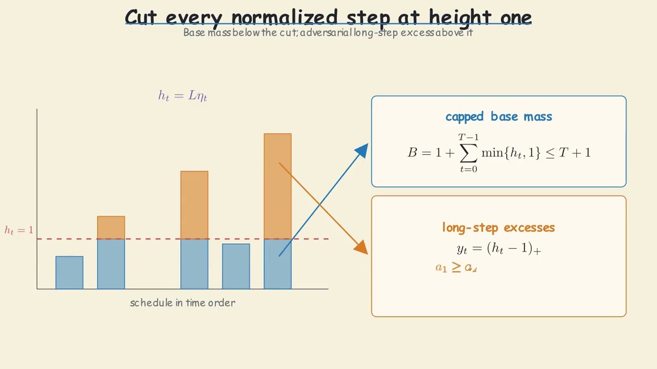
[02:49](https://www.youtube.com/watch?v=ypPY5Z6yQP0&t=169s) Normalized Steps, Base Mass, and Long-Step Excess

The technical proof begins by normalizing each stepsize by the Lipschitz constant, defining dimensionless step lengths:

$$h_t = L \eta_t$$

The schedule is then visualized as a sequence of vertical bars of height $h_t$. The proof slices every bar horizontally at height $1$. The capped lower portions—those lying in the interval $[0, 1]$—are summed together along with an initial unit offset to form the total "base mass":

$$B = 1 + \sum_{t=0}^{T-1} \min(h_t, 1)$$

Any portion of a step extending above height $1$ is defined as an excess:

$$y_t = \max(0, h_t - 1)$$

A step is formally classified as a "long step" if and only if its excess $y_t$ is strictly positive, with $r$ denoting the total count of such long steps.

If a schedule contains no large excesses, defeating it is mathematically straightforward: an elementary, low-dimensional convex construction reproduces the standard $\mathcal{O}(T^{-1})$ lower bound. The adversary's true technical hurdle is defeating schedules loaded with arbitrarily large, irregular step spikes distributed in an arbitrary temporal order.

---

[03:29](https://www.youtube.com/watch?v=ypPY5Z6yQP0&t=209s) The Moreau-Envelope Hard Instance and Orthogonal Anchors

To neutralize arbitrary spikes, the adversary selects a subset of long steps preserving their original chronological order, partitioning the time horizon into distinct operational blocks. Each block $i$ is assigned an orthogonal anchor point $x_i$ and a corresponding gradient vertex $g_i$. Within block $i$, ordinary short steps move down the ray from $x_i$ along the direction $-g_i$. The block's terminal selected long step is then precisely tuned: its excess magnitude launches the iterate off the current ray to land on the next anchor point $x_{i+1}$, aligned along a completely fresh coordinate axis.

``` Coordinate Axis i+1 ^ | Target Anchor x_{i+1} | * | / | / (Selected long step jumps | / across coordinate axes) | / | / +-------------------*------------------------> Coordinate Axis i x_i - η g_i [Ordinary steps move along ray -g_i] ```

To make this artificial trajectory the true path of gradient descent on a valid, smooth convex objective, the authors employ the Moreau envelope. The adversary defines a set $K$ as the convex hull of the origin and all gradient vertices:

$$K = \operatorname{conv}(\{0\} \cup \{g_1, g_2, \dots, g_m\})$$

The adversarial objective $f$ is then constructed as the Moreau envelope of the support function of $K$, denoted $\sigma_K$. By the classical properties of Moreau envelopes, $f$ is guaranteed to be smooth and convex, and its gradient at any point evaluates to the metric projection onto $K$:

$$\nabla f(x) = \operatorname{proj}_K(x)$$

By establishing precise projection comparisons across the geometric domain, the adversary ensures that throughout the entirety of block $i$, the projection of the iterate onto $K$ remains identical to the single vertex $g_i$, keeping the gradient constant along the ray until the spike transitions the iterate into the next orthogonal subspace.

---

[04:17](https://www.youtube.com/watch?v=ypPY5Z6yQP0&t=257s) Converting Multi-Dimensional Geometry into a Scalar Chain

With the trajectory constrained to orthogonal coordinate axes, the adversary reduces the multi-dimensional vector dynamics into an explicit scalar chain. Each anchor point is expressed as $x_i = \lambda_i e_i$, where $e_i$ is a standard basis vector and $\lambda_i$ denotes the anchor amplitude. Across transitions, the consecutive squared amplitudes scale according to multiplicative contraction factors $\chi_i$:

$$\lambda_{i+1}^2 = \chi_i \lambda_i^2$$

At the final block $m$, the objective suboptimality gap is given by:

$$\frac{\lambda_m^2}{2 h_m}$$

Normalizing the initial amplitude to $\lambda_0 = 1$ and chaining the transitions yields a closed-form scalar expression for the terminal objective gap:

$$\frac{1}{2 h_m} \prod_{i=0}^{m-1} \chi_i$$

The adversary maximizes this expression over all admissible index selections and block partitions, yielding a scalar functional $\mathcal{C}(T)$ that depends solely on the stepsize schedule. The remaining analytical task is to establish that no arrangement of long-step excesses can drive this functional below the target error floor.

---

[05:07](https://www.youtube.com/watch?v=ypPY5Z6yQP0&t=307s) Erasing Temporal Order via Path Matchings

Temporal order poses the primary analytical barrier because each step transition strongly couples neighboring blocks. To break these chronological dependencies, the proof sorts all positive excesses $y_t$ in descending order, from largest to smallest. For any index $q$, let $D_q$ denote the cumulative base mass $B$ augmented by the unselected excess tail.

For the $q$ largest excesses, a budget equalization argument converts the reciprocal chain value into the edge product of a weighted path graph. The edges of this path are partitioned into two disjoint matchings: - The set of odd-indexed edges forms the first matching. - The set of even-indexed edges forms the second matching.

By replacing the chronological product with the cost of an optimal order-free matching, the adversary decouples the step sizes from their execution timestamps. This leads to the fundamental lower bound on the schedule functional:

$$\mathcal{C}(T) \ge \frac{q}{2 D_q (q - 1)} \mu_q^q$$

Whenever the matching metric $\mu_q$ falls below $1$, its reciprocal power generates an exponentially growing factor, establishing a floor under the optimization error.

---

[05:51](https://www.youtube.com/watch?v=ypPY5Z6yQP0&t=351s) Deriving the 1.9319 Threshold via Lyapunov Potentials

The analysis bifurcates into two complementary regimes governed by a density statistic, $Z_q$: - **Matching Contraction Branch**: When $Z_q$ is small, the bipartite matching branch contracts effectively, yielding the desired error bound directly. - **Lyapunov Residual Branch**: When $Z_q$ is large, an adjacent-rank recursion combined with a discrete Lyapunov potential restricts how rapidly the residual schedule mass can accumulate.

Both branches are parameterized by the scalar:

$$\theta = \frac{1}{p^2 - 1}$$

To guarantee that the matching branch contracts and matches the Lyapunov decay, the parameter $\theta$ must satisfy the quadratic stability inequality:

$$2\theta + 2\theta^2 < 1$$

To solve for the critical exponent $p$, substitute $\theta = 1/z$ where $z = p^2 - 1$:

$$\frac{2}{z} + \frac{2}{z^2} < 1$$

Multiplying through by the positive denominator $z^2$ yields the characteristic quadratic equation:

$$z^2 - 2z - 2 > 0$$

Applying the quadratic formula to find the positive root gives:

$$z = \frac{2 + \sqrt{4 - 4(1)(-2)}}{2} = 1 + \sqrt{3}$$

Re-substituting $z = p^2 - 1$:

$$p^2 - 1 > 1 + \sqrt{3} \implies p^2 > 2 + \sqrt{3}$$

Taking the positive square root reveals the critical threshold:

$$p > \sqrt{2 + \sqrt{3}} \approx 1.93192$$

Any exponent $p$ above this value guarantees the existence of an adversarial objective that halts plain gradient descent.

``` Quadratic inequality in z = p² - 1: z² - 2z - 2 > 0 Roots: z = 1 ± √3

Positive branch: z > 1 + √3 p² - 1 > 1 + √3 p² > 2 + √3 p > √(2 + √3) ≈ 1.93185... (1.9319) ```

---

[06:39](https://www.youtube.com/watch?v=ypPY5Z6yQP0&t=399s) Scope Limitations, the Silver Gap, and Lean 4 Formalization

The theorem's conclusions are mathematically sharp, but its scope is precisely delimited. The lower bound strictly rules out achieving an exponent above $1.9319$ via predetermined, nonnegative scalar stepsize schedules on the unmodified last iterate of smooth convex objectives.

``` Convergence Exponent Spectrum (Negative Power of T) 0.0 1.0 1.2715 1.9319 2.0 |--------------|-------------------|-------------------|--------------| Standard GD Silver Steps Proven Lower Nesterov Full (Constant η) (Fractal Spikes) Bound Floor Acceleration \_________________/ ^ Open Gap (~0.66) ```

This leaves a substantial open gap between the best known constructive upper bound—the silver schedule at approximately $1.2715$—and the proven lower bound threshold of $1.9319$. Whether the true optimal exponent for predetermined plain gradient descent lies near $1.27$, reaches $1.93$, or sits somewhere in between remains an open question in optimization theory.

Crucially, the theorem does not apply to: - Best-iterate selection rules (evaluating $\min_{t \le T} f(x_t)$ rather than the terminal iterate $x_T$). - Strongly convex objectives. - Nonconvex optimization problems. - Adaptive or line-search algorithms (such as Polyak stepsizes or backtracking). - Randomized or stochastic step selection rules. - Negative step sizes. - Momentum-based methods (such as Heavy-Ball or Nesterov acceleration).

Every step of the finite-horizon proof has been mechanically verified in the Lean 4 interactive theorem prover without introducing custom project-defined axioms. The enduring theoretical takeaway is clear: while intelligent stepsize scheduling can accelerate plain gradient descent well beyond its classical $\mathcal{O}(T^{-1})$ baseline, "scheduling alone is not full acceleration." Reaching the optimal $\mathcal{O}(T^{-2})$ rate fundamentally requires state-carrying mechanisms such as momentum.

## Notable quotes > [00:01](https://www.youtube.com/watch?v=ypPY5Z6yQP0&t=1s) The term "lower bound" often sounds reassuring to an outsider, almost like a performance guarantee promising that an algorithm will perform at least reasonably well. In computational complexity and optimization theory, however, it means the exact opposite: an inescapable, adversarial error floor.

> [00:01](https://www.youtube.com/watch?v=ypPY5Z6yQP0&t=1s) is plain gradient descent inherently weaker than momentum-accelerated methods, or can it match them if equipped with a sufficiently clever, non-constant stepsize schedule?

> [00:01](https://www.youtube.com/watch?v=ypPY5Z6yQP0&t=1s) because any exponent p > 1.9319 produces an error floor that decays strictly slower than T^{-2}, no fixed scalar stepsize schedule can allow vanilla gradient descent to uniformly replicate Nesterov acceleration.

> [01:24](https://www.youtube.com/watch?v=ypPY5Z6yQP0&t=84s) The adversary exploits full advance knowledge of the schedule and the horizon to weave an instance specifically tuned to foil that exact step sequence.

> [02:06](https://www.youtube.com/watch?v=ypPY5Z6yQP0&t=126s) varying step sizes does genuine work: non-constant schedules are not naive heuristics.

> [02:06](https://www.youtube.com/watch?v=ypPY5Z6yQP0&t=126s) silver steps genuinely accelerate plain gradient descent, boosting the convergence rate from \mathcal{O}(T^{-1}) to approximately \mathcal{O}(T^{-1.2715}).

> [02:06](https://www.youtube.com/watch?v=ypPY5Z6yQP0&t=126s) The paper answers that question in the negative, showing that the acceleration plateaus well before reaching the Nesterov frontier.

> [02:49](https://www.youtube.com/watch?v=ypPY5Z6yQP0&t=169s) The adversary's true technical hurdle is defeating schedules loaded with arbitrarily large, irregular step spikes distributed in an arbitrary temporal order.

> [06:39](https://www.youtube.com/watch?v=ypPY5Z6yQP0&t=399s) scheduling alone is not full acceleration.

> [06:39](https://www.youtube.com/watch?v=ypPY5Z6yQP0&t=399s) Reaching the optimal \mathcal{O}(T^{-2}) rate fundamentally requires state-carrying mechanisms such as momentum.

## Mentioned arXiv:2608.10418, Yurii Nesterov, Nesterov acceleration, Lean 4, Moreau envelope, Polyak stepsizes, Heavy-Ball, Xiaol.x

## Video description What exactly does the lower bound in arXiv:2608.10418 bound, and why does it matter?

This video explains the paper’s main result: for every predetermined, nonnegative scalar stepsize schedule, there exists a smooth convex objective whose final gradient-descent error is at least

c_p L R² times (T plus 1) to the power minus p,

where p is strictly greater than the threshold square root of 2 plus square root of 3, approximately 1.9319.

The bound concerns the worst-case last-iterate objective error, f(x_T) minus f(x_star). It is not a bound on the stepsize, runtime, or every objective.

The result matters because the classical accelerated rate of order T to the power minus 2 applies to general first-order methods and does not distinguish Nesterov acceleration from plain gradient descent. This paper proves that stepsize scheduling alone cannot make plain GD uniformly achieve that rate.

The video covers:

- Textbook GD and its order T to the power minus 1 rate - The silver schedule and its exponent approximately 1.2715 - The adversarial quantifier order - Capped mass and long-step excesses - The Moreau-envelope hard instance - Orthogonal-anchor geometry - The path-matching reduction - Matching and Lyapunov proof branches - The derivation of the 1.9319 threshold - The remaining gap between 1.2715 and 1.9319 - The authors’ Lean 4 formalization

The theorem applies to predetermined schedules, smooth convex objectives, and the unmodified last iterate. It does not cover adaptive or randomized steps, signed steps, momentum, line search, best-iterate outputs, strongly convex objectives, or nonconvex optimization.

Paper: https://arxiv.org/abs/2608.10418

Chapters

00:00 The lower bound is an error floor 00:41 Why the exponent matters 01:24 The adversarial quantifiers 02:06 Silver steps genuinely accelerate GD 02:49 Base mass and long-step excess 03:29 Moreau-envelope hard instance 04:17 Geometry becomes a scalar chain 05:07 Two matchings erase temporal order 05:51 Deriving the threshold 06:39 What remains open

[Source](https://www.youtube.com/watch?v=ypPY5Z6yQP0)

中文简报

研究证实固定步长调度无法匹敌Nesterov加速速率预设标量步长调度无法使朴素梯度下降加速至Nesterov的速率，因为对抗方始终能在高于1.9319的任意指数处强加误差下界，这证明完全加速从根本上需要动量。该视频阐述了为何预设标量步长调度无法让朴素梯度下降达到Nesterov加速的$\mathcal{O}(T^{-2})$速率，并确立了指数为$p > \sqrt{2 + \sqrt{3}} \approx 1.9319$的误差下界。尽管诸如白银调度（silver schedule）等非常数技术确实能将梯度下降加速至约$\mathcal{O}(T^{-1.2715})$，但一种在正交锚点上利用Moreau包络的对抗性构造利用了任意步长尖峰来限制迭代点。通过将轨迹几何转化为标量链，并借助二分路径匹配和离散Lyapunov势函数消除时间排序，作者推导出了一个阻碍收敛的二次稳定性阈值。该结果已在Lean 4中完成全形式化，证实了尽管调度可以改善标准梯度下降，但要实现完全加速，从根本上仍然需要动量等具有状态保留机制的方法。一项新的理论结果表明，对于任何预设的非负标量步长调度，对抗方都可以构建一个光滑凸函数，迫使朴素梯度下降的末次迭代误差衰减速度对于任意$p > \sqrt{2 + \sqrt{3}} \approx 1.9319$均不快于$c_p L R^2 (T+1)^{-p}$。 (0:01) 由于该下界对所有$p > 1.9319$均成立，这严格证明了单靠步长调度无法让标准梯度下降一致地达到Nesterov的$\mathcal{O}(T^{-2})$加速速率。 (0:41) 在目前已知最快的预设调度（即达到$\mathcal{O}(T^{-1.2715})$的分形白银调度）与已证实的$1.9319$不可能壁垒之间，仍存在显著的理论差距。 (6:39) 结合了Moreau包络、二分路径匹配以及离散Lyapunov势函数的整个有限时域下界证明，已在Lean 4中完成了机械化验证，且未使用自定义公理。 (6:39)

Reading summary

According to research presented from arXiv:2608.10418, plain gradient descent equipped with any predetermined, nonnegative scalar stepsize schedule cannot achieve Nesterov's accelerated convergence rate of O(T^-2) on smooth convex functions, encountering an adversarial last-iterate error floor that scales as (T + 1)^-p for any exponent p strictly greater than √(2 + √3) ≈ 1.9319. Inescapable Lower Bounds and Adversarial Schedules (0:01) Classical first-order oracle lower bounds developed by Yurii Nesterov scale as O(T^-2), but because momentum-accelerated methods match this rate, classical complexity theory cannot determine whether standard gradient descent could also achieve it through a sufficiently clever stepsize schedule. The presented theorem resolves this separation: because any exponent p > 1.9319 decays strictly slower than T^-2, predetermined scalar stepsize sequences are fundamentally incapable of closing the efficiency gap to Nesterov acceleration. The result operates through an asymmetric quantifier sequence. The observer first fixes an exponent p > √(2 + √3) and a problem-independent constant c_p > 0. The algorithm designer then chooses the time horizon T, the Lipschitz constant L, the initial distance R, the starting point x_0, and the complete step sequence {η_t}. Only after inspecting the entire schedule does the adversary step in to construct an L-smooth convex objective function f in dimension d ≤ T + 1 that forces the last-iterate suboptimality gap f(x_T) - f(x*) to remain above c_p L R^2 (T + 1)^-p. Silver Step Acceleration and Schedule Decomposition (2:06) Proving a lower bound beyond O(T^-1) is challenging because non-constant stepsize schedules provide genuine acceleration. While constant step sizes limit gradient descent to O(T^-1), recent constructions such as the fractal-like 'silver stepsize schedule' boost convergence to roughly O(T^-1.2715) by alternating short steps with aggressive, non-monotonic step spikes. This raised the open question of whether more sophisticated patterns of spikes could bridge the remaining gap to 2.0. To analyze arbitrary spike patterns, the authors normalize steps as h_t = L η_t and slice each step horizontally at height 1. The capped portions in [0, 1] sum into a base mass B = 1 + ∑ min(h_t, 1), while any height exceeding 1 is designated an excess y_t = max(0, h_t - 1). While schedules lacking significant excess can be bounded by standard O(T^-1) techniques, the primary technical hurdle is neutralising schedules featuring arbitrarily ordered, extreme step spikes. Moreau Envelopes and Orthogonal Coordinate Chains (3:29) To counter arbitrary schedules, the adversary selects a subset of long steps and divides the horizon into blocks associated with orthogonal anchor points x_i and gradient vertices g_i. Ordinary short steps traverse down the ray from x_i along -g_i, while the terminal long step of the block spikes the iterate onto the subsequent anchor x_{i+1} situated on a completely fresh coordinate axis. To ensure this geometric trajectory constitutes valid gradient descent on an L-smooth convex objective, the adversary defines f as the Moreau envelope of the support function of K = conv({0} ∪ {g_1, ..., g_m}). Under the properties of Moreau envelopes, the gradient equals the metric projection onto K, holding the gradient constant along each coordinate ray. Squared anchor amplitudes contract across transitions by factors χ_i, converting multi-dimensional geometry into a closed-form scalar chain functional C(T) = (1 / 2h_m) ∏ χ_i that bounds the final suboptimality gap. Decoupling Order and the 1.9319 Threshold (5:07) Because temporal ordering couples neighboring steps, the proof sorts all positive excesses in descending order and models the reciprocal chain functional as the edge product of a weighted path graph. Splitting this path into two disjoint matchings—odd-indexed and even-indexed edges—decouples step magnitudes from chronological timestamps, bounding the schedule functional by an order-free matching metric μ_q. The analysis then bifurcates based on a density statistic Z_q. When Z_q is small, the bipartite matching branch contracts directly; when Z_q is large, an adjacent-rank recursion paired with a discrete Lyapunov potential restricts residual schedule mass accumulation. Balancing both regimes requires the parameter θ = 1 / (p^2 - 1) to satisfy the stability inequality 2θ + 2θ^2 < 1. Substituting z = p^2 - 1 yields the characteristic polynomial z^2 - 2z - 2 > 0, whose positive root z = 1 + √3 establishes the threshold exponent p > √(2 + √3) ≈ 1.9319. The authors emphasize that this lower bound is delimited to the unmodified last-iterate error of predetermined scalar stepsize schedules on smooth convex objectives; it does not apply to momentum, adaptive methods, line searches, or best-iterate selections. Mechanically formalized in Lean 4 without custom axioms, the result proves that scheduling alone cannot replicate Nesterov acceleration, while leaving an open theoretical gap between the constructive silver schedule rate (~1.2715) and the 1.9319 impossibility floor.

Source quotes

[0:01] The term "lower bound" often sounds reassuring to an outsider, almost like a performance guarantee promising that an algorithm will perform at least reasonably well. In computational complexity and optimization theory, however, it means the exact opposite: an inescapable, adversarial error floor. [0:01] is plain gradient descent inherently weaker than momentum-accelerated methods, or can it match them if equipped with a sufficiently clever, non-constant stepsize schedule? [0:01] because any exponent p > 1.9319 produces an error floor that decays strictly slower than T^{-2}, no fixed scalar stepsize schedule can allow vanilla gradient descent to uniformly replicate Nesterov acceleration. [1:24] The adversary exploits full advance knowledge of the schedule and the horizon to weave an instance specifically tuned to foil that exact step sequence. [2:06] varying step sizes does genuine work: non-constant schedules are not naive heuristics. [2:06] silver steps genuinely accelerate plain gradient descent, boosting the convergence rate from \mathcal{O}(T^{-1}) to approximately \mathcal{O}(T^{-1.2715}). [2:06] The paper answers that question in the negative, showing that the acceleration plateaus well before reaching the Nesterov frontier. [2:49] The adversary's true technical hurdle is defeating schedules loaded with arbitrarily large, irregular step spikes distributed in an arbitrary temporal order. [6:39] scheduling alone is not full acceleration. [6:39] Reaching the optimal \mathcal{O}(T^{-2}) rate fundamentally requires state-carrying mechanisms such as momentum.

Original transcript

[0:01] The phrase lower bound can sound like a [0:02] guarantee that an algorithm will be [0:04] good. Here it means the opposite, an [0:07] unavoidable error floor. Pick any [0:10] non-negative step size schedule before [0:13] seeing the objective. After T steps, an [0:18] adversary can choose a smooth convex [0:20] function where the final point still has [0:22] objective gap at least C sub P times LR [0:24] squared times T plus 1 to the minus P. [0:28] The quantity being bounded is the last [0:31] iterate error, f of x t minus f star. It [0:35] is not a bound on the step size, and it [0:37] does not say every objective is hard. [0:40] The usual first-order oracle lower bound [0:43] is proportional to T to the minus 2, and [0:47] Nesterov acceleration reaches that rate. [0:49] Because the old statement applies to [0:51] every first-order method, it cannot [0:53] reveal whether plain gradient descent is [0:56] weaker. The new exponent does. [0:59] For every P just above 1.9319, [1:04] some objective forces plain gradient [1:07] descent to have error at least a [1:09] constant times T to the minus P. That [1:12] floor decays more slowly than T to the [1:15] minus 2, so no predetermined [1:18] non-negative scalar schedule can [1:20] uniformly match accelerated methods. [1:24] The theorem is a game with a strict move [1:26] order. First, choose the exponent P. [1:29] Then a positive constant C sub P exists. [1:32] Next, the designer chooses T, L, R, the [1:36] initialization, and every step size. [1:39] Only afterward does the adversary choose [1:42] a dimension no larger than T plus 1, a [1:45] smooth convex function, and a minimizer [1:48] exactly distance R away. The resulting [1:52] gradient descent trajectory respects the [1:54] chosen schedule, yet its final gap meets [1:57] the lower bound. This quantifier order [1:59] is preserved in the author's lean [2:01] formalization. The hard function may [2:03] depend on the schedule and the horizon. [2:07] The schedule being challenged is not [2:09] naive. The silver construction is [2:11] genuinely clever. It's normalized steps [2:15] begin square root of two, two, square [2:17] root of two, then a larger spike, and [2:20] the pattern repeats recursively. [2:23] Those rare long steps may temporarily [2:25] increase the objective, but they improve [2:27] the final rate from T to the minus one [2:30] to roughly T to the minus one point two [2:32] seven one five. [2:34] The paper asks whether even more [2:36] ingenious predetermined spikes could [2:40] reach exponent two. Its answer is no, [2:43] although it does not identify the best [2:46] possible exponent. [2:48] The proof normalizes each step as HT [2:51] equals LA to T. It cuts every bar at [2:55] height one. The capped pieces contribute [2:57] base mass B equal to one plus the sum of [3:01] the capped steps. The pieces above one [3:04] are excesses YT, and a step is called [3:07] long exactly when its excess is [3:09] positive. Let R count those long steps. [3:13] If there are no large excesses, an [3:16] elementary hard instance already gives [3:18] the usual order one over T floor. The [3:21] challenge is to defeat schedules with [3:24] many arbitrarily large spikes in any [3:26] temporal order. [3:28] Select some long steps in their original [3:31] order. They divide time into blocks. [3:33] Block I receives an orthogonal anchor XI [3:37] and a gradient vertex GI. Ordinary steps [3:40] move along the ray from XI in direction [3:43] minus GI. The selected long step is [3:46] tuned to land exactly on the next anchor [3:49] on a fresh coordinate axis. To realize [3:52] this artificial path with a legitimate [3:54] smooth convex objective, define K as the [3:58] convex hull of zero and all gradient [4:01] vertices, then take the Moreau envelope [4:04] of K's support function. Its gradient is [4:08] projection onto K. Projection [4:11] comparisons keep that gradient equal to [4:13] GI throughout the block. [4:16] Write each anchor as lambda I times an [4:19] orthogonal basis vector. [4:22] Consecutive squared amplitudes satisfy [4:24] lambda I plus one squared equals chi I [4:28] times lambda I squared. At the terminal [4:31] block, the objective gap is lambda M [4:34] squared divided by 2 HM. Starting from [4:38] lambda zero equal to one, substitution [4:42] turns the geometry into one over 2 HM [4:45] times the product of all chi factors. [4:48] The paper maximizes this quantity over [4:51] every admissible selection and block [4:53] construction producing a scalar [4:56] functional CT of the schedule. The [4:59] remaining proof must show that no [5:02] arrangement of long step excesses can [5:04] make this functional too small. [5:07] Temporal order is the main obstacle [5:08] because each transition couples [5:10] neighboring blocks. Sort the positive [5:12] excesses from largest to smallest and [5:14] define DQ as the base mass plus the [5:17] unselected tail. For the Q largest [5:20] excesses, budget equalization turns the [5:22] reciprocal chain value into the edge [5:25] product of a weighted path. Odd edges [5:28] form one matching, even edges form [5:30] another. Replacing each chronological [5:33] matching by its optimal order-free cost [5:35] gives CT at least Q divided by 2 DQ Q [5:40] minus 1 and mu Q to the Q. If mu Q is [5:44] below one, its reciprocal power creates [5:47] a rapidly growing favorable factor. [5:51] One density statistic Z Q controls the [5:55] matching cost. If Z is small, the [5:58] matching branch contracts. Otherwise, [6:00] the adjacent rank recursion and a [6:02] Lyapunov potential control how quickly [6:05] residual schedule mask can grow. The two [6:08] branches use data equal to 1 over P [6:11] squared minus 1. [6:13] Matching requires 2 theta plus 2 theta [6:16] squared to be strictly less than 1. [6:18] Substitute theta, multiply by the [6:21] positive denominator, and obtain Z [6:24] squared minus 2 Z minus 2 greater than [6:27] 0, where Z equals P squared minus 1. [6:30] Um [6:31] the positive root gives P greater than [6:33] the square root of 2 plus square root of [6:35] 3, 1.9319. [6:40] >> [gasps] [6:40] >> The conclusion is sharp in scope. [6:42] Predetermined non-negative steps alone [6:45] cannot guarantee any exponent above [6:48] 1.9319, [6:49] so they cannot reach the optimal [6:51] exponent 2. The best construction still [6:53] guarantees only 1.2715, [6:56] leaving a wide open interval. The [6:58] theorem concerns the unmodified last [7:01] iterate on smooth convex objectives. It [7:04] does not cover the best iterate strong [7:06] convexity, adaptive or randomized rules, [7:10] negative steps, momentum, or line [7:11] search. The authors' lean development [7:14] verifies the complete finite horizon [7:16] statement without project defined [7:18] axioms. [7:20] The lasting lesson is a separation. [7:23] Scheduling helps plain gradient descent, [7:25] but scheduling alone is not full [7:27] acceleration.