Transformers Are Wide—But Their Feedback Is Narrow | Full-Bandwidth Transformer Explained

Xiaol.x

AI-assisted summary of Transformers Are Wide—But Their Feedback Is Narrow | Full-Bandwidth Transformer Explained — original source. Check the original for full context.

Source published: 2026-08-23

Key ideas

The Full-Bandwidth Transformer addresses the bottleneck in standard autoregressive decoding by feeding the prior top-layer state directly into the next token's input layer via an asymmetric gate, expanding reachability from a triangle Θ(Tℓ) to a rectangle Θ(TL). (0:00)
To preserve parallel pretraining without sequential recurrence, the architecture uses a Jacobi-style multi-pass training schedule, decoupling sequence length from feedback depth. (5:56)
Replacing just 3% of two-pass training batches with three-pass batches prevents hidden state oscillations and stabilizes validation loss across up to 30 iterative passes. (7:39)
Linear probing shows near-perfect decodability of global context features at layer zero under latent feedback, though base-model gains tend to diminish after standard instruction tuning. (8:30)

Detailed notes

## Background Published on YouTube by channel Xiaol.x on August 23, 2026, this visual lesson explains the mathematics, intuitions, and training mechanics behind the Full-Bandwidth Transformer paper (arXiv:2608.08888). According to the video description, it illustrates how latent feedback recirculates top-layer hidden states into the next token's input to overcome the narrow discrete bottleneck of standard autoregressive decoding.

## TL;DR Standard autoregressive transformers squeeze their rich, high-dimensional top-layer hidden states through a single sampled discrete token, leaving past computations 'depth-frozen' in the KV cache without the ability to receive fresh computational depth. The Full-Bandwidth Transformer addresses this by introducing asymmetric latent feedback, where the previous top-layer state provides the value and the incoming token embedding acts as a multiplicative gate, expanding reachability from a triangle $\Theta(T\ell)$ to a rectangle $\Theta(TL)$ while keeping serial depth constant. To bypass the sequential training bottleneck of recurrent feedback, the model uses Jacobi-style multi-pass parallel training with a prefix mix-in objective. Adding as little as 3% three-pass batches stabilizes hidden state updates into a contraction-like plateau over extended inference passes, enabling high linear probe decodability at layer zero and outperforming standard decoding baselines up to 1B parameters.

## Atmosphere & style The presentation carries the deliberate, lucid precision of an advanced graduate lecture or formal theoretical walkthrough, complemented by Lean 4 visualizations and clean architectural diagrams. It maintains a measured, intellectually rigorous tone that methodically dismantles common assumptions—such as the belief that the KV cache already solves depth routing—before rebuilding the solution from first principles. The narrative arc moves smoothly from diagnostic friction to elegant algebraic formulation, tempering enthusiasm with clear-eyed scientific humility regarding heuristic schedules, model scale boundaries, and instruction-tuning limitations.

## Bulletin - [00:00](https://www.youtube.com/watch?v=aT3DSgHKMOs&t=0s) The Full-Bandwidth Transformer addresses the bottleneck in standard autoregressive decoding by feeding the prior top-layer state directly into the next token's input layer via an asymmetric gate, expanding reachability from a triangle Θ(Tℓ) to a rectangle Θ(TL). - [05:56](https://www.youtube.com/watch?v=aT3DSgHKMOs&t=356s) To preserve parallel pretraining without sequential recurrence, the architecture uses a Jacobi-style multi-pass training schedule, decoupling sequence length from feedback depth. - [07:39](https://www.youtube.com/watch?v=aT3DSgHKMOs&t=459s) Replacing just 3% of two-pass training batches with three-pass batches prevents hidden state oscillations and stabilizes validation loss across up to 30 iterative passes. - [08:30](https://www.youtube.com/watch?v=aT3DSgHKMOs&t=510s) Linear probing shows near-perfect decodability of global context features at layer zero under latent feedback, though base-model gains tend to diminish after standard instruction tuning.

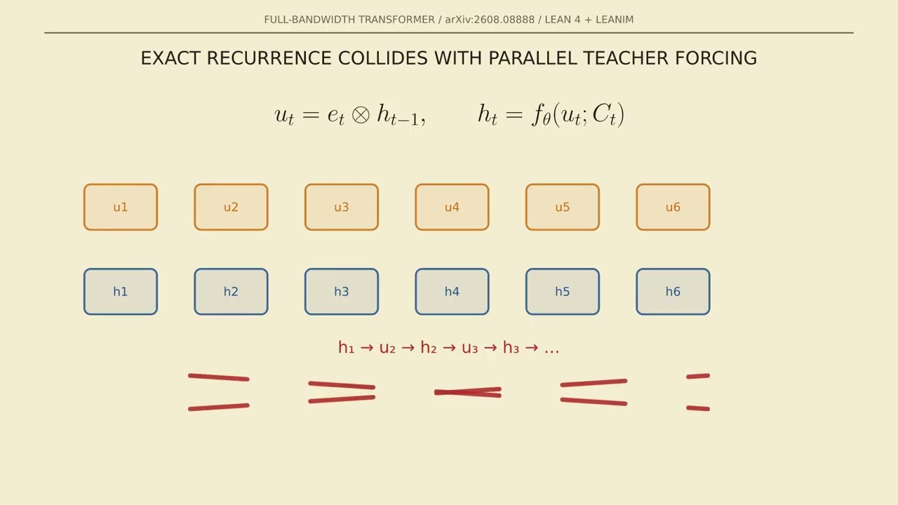
## Key takeaways - [00:00](https://www.youtube.com/watch?v=aT3DSgHKMOs&t=0s) Standard transformers suffer from an architectural paradox: attention is wide across past tokens, but the feedback between sequential decoding steps is squeezed through a single discrete token. - [00:50](https://www.youtube.com/watch?v=aT3DSgHKMOs&t=50s) The KV cache preserves key and value vectors across context but leaves computation 'depth-frozen' because attention layers cannot route deeper past representations downward to lower layers. - [01:44](https://www.youtube.com/watch?v=aT3DSgHKMOs&t=104s) Chain-of-thought prompting functions as a discrete scratchpad, transmitting at most log2(|V|) bits per token rather than leveraging the rich, continuous d-dimensional activation vector. - [02:37](https://www.youtube.com/watch?v=aT3DSgHKMOs&t=157s) The asymmetric latent-feedback gate multiplies the projected prior top-layer state by a sigmoid-gated token embedding, preventing the model from degenerating into a token-only bypass shortcut. - [03:23](https://www.youtube.com/watch?v=aT3DSgHKMOs&t=203s) Latent feedback introduces no new factual information; its primary advantage is computational accessibility, enabling finished computations to receive a fresh depth budget through the full transformer stack. - [04:17](https://www.youtube.com/watch?v=aT3DSgHKMOs&t=257s) Direct latent routing expands computational reachability from a causal triangle of volume Θ(Tℓ) to a full rectangle of Θ(TL), all while keeping serial execution depth per token at O(L). - [05:07](https://www.youtube.com/watch?v=aT3DSgHKMOs&t=307s) Exact recurrent training destroys sequence-level parallel teacher forcing, creating a dilemma for training latent feedback on large datasets. - [05:56](https://www.youtube.com/watch?v=aT3DSgHKMOs&t=356s) Jacobi-style temporal parallelism restores training efficiency by running K iterative forward passes across the sequence, where each pass shifts and fuses the previous pass's top states in parallel. - [06:48](https://www.youtube.com/watch?v=aT3DSgHKMOs&t=408s) The multi-pass training loss preserves first-pass prefill behavior alongside feedback passes, and a prefix mix-in strategy matches the mixed plain-and-feedback input distribution seen at inference. - [07:39](https://www.youtube.com/watch?v=aT3DSgHKMOs&t=459s) A tiny injection of deeper training—swapping just 3% of two-pass batches with three-pass batches—induces contraction-mapping-like stability over extended recurrence horizons. - [08:30](https://www.youtube.com/watch?v=aT3DSgHKMOs&t=510s) Linear probes at layer zero confirm immediate access to sequence completion tracking and memory recall, demonstrating representational availability of prior top-layer computation. - [09:28](https://www.youtube.com/watch?v=aT3DSgHKMOs&t=568s) The architecture introduces depth renewal with minimal overhead—only two projection matrices—though evaluated scales currently stop at 1 billion parameters and empirical gains attenuate after instruction tuning.

## Detailed walkthrough ### [00:00](https://www.youtube.com/watch?v=aT3DSgHKMOs&t=0s) Wide Attention, Narrow Feedback

Transformers exhibit a fundamental architectural paradox: while self-attention permits a model to look across thousands of tokens in context, the channel connecting consecutive decoding steps is squeezed through an extraordinarily narrow bottleneck. At any step, the previous token's top layer retains a high-dimensional vector packed with nuanced computational state—capturing internal uncertainty, partial arithmetic calculations, and emerging generation plans. In standard autoregressive decoding, however, the vocabulary projection head flattens this rich continuous vector into a discrete probability distribution, samples a single word token, and passes only that sampled token's lookup embedding back into the input layer for the next step.

```mermaid flowchart TD accTitle: Standard Decoding vs Full-Bandwidth Latent Feedback accDescr: Diagram contrasting how standard decoding compresses the top-layer hidden state through a single discrete token versus the latent-feedback gating mechanism.

subgraph Standard["Standard Decoding (Discrete Bottleneck)"] H_prev["Top Hidden State: h_(t-1)"] --> Head["Vocab Projection Head"] Head --> Sample["Sampled Word Token: w_t"] Sample --> Embed["Token Embedding: e_t"] Embed --> NextL0["Next Layer 0 Input: x_t"] end

subgraph LatentFeedback["Full-Bandwidth Latent Feedback"] TopH["Top State: h_(t-1)"] --> ValueBranch["Value Branch: W_U * h_(t-1)"] TokE["Token Embedding: e_t"] --> GateBranch["Gate Branch: σ(W_G * e_t)"] ValueBranch --> Mult["Hadamard Product (⊙)"] GateBranch --> Mult Mult --> U_t["Fused Input: u_t"] end ```

The resulting system is "horizontally wide across tokens, but vertically narrow across steps." The core dilemma is not whether representations of past inputs exist, but whether fully processed, top-tier computation can be recirculated back to the foundation of the network to receive a brand-new depth budget.

[00:50](https://www.youtube.com/watch?v=aT3DSgHKMOs&t=50s) Why the KV Cache Leaves Computation "Depth-Frozen"

A frequent initial reaction to this diagnosis points to the key-value (KV) cache: does the KV cache not already preserve the model's past activations across context? While the cache reliably preserves key and value vectors at each individual layer, its geometry imposes strict constraints on computational routing. During the computation of token $t$ at layer $\ell$, attention is restricted to reading states generated at earlier positions $t'$ at or below depth $\ell$. It cannot reach into deeper past layers and transport those high-level representations downward to lower layers.

Because the top-layer output has no higher attention layer above it in which to be stored, the model's reachable computational set is fundamentally triangular—spanning prior tokens $t' < t$ and strictly lower depths $\ell' < \ell$, with a total volume scaling as $\Theta(T \ell)$. At the foundational input layer ($\ell = 0$), this reachable history shrinks to virtually nothing. Persistence of activations in memory is therefore entirely distinct from renewing their computational depth; the earlier work remains what the paper characterizes as "depth frozen."

[01:44](https://www.youtube.com/watch?v=aT3DSgHKMOs&t=104s) Chain of Thought as a Discrete Scratchpad

Historically, autoregressive language models circumvent this vertical barrier through chain-of-thought (CoT) prompting and reasoning traces. To pass a partial remainder, sub-goal, or unresolved hypothesis forward in time, the model is forced to verbalize it explicitly as intermediate text tokens that future decoding positions can read through attention. - For instance, when dividing $137 / 500$, an extended trace writes out intermediate long division steps sequentially before arriving at $0.274$. - While effective, this communication protocol relies on a discrete interface: each generated token can distinguish at most $|V|$ possibilities, transmitting roughly $\log_2 |V|$ bits of information. - By contrast, the pre-sampling top-layer activation holds $d$ continuous coordinates. While not carrying infinite information, standard decoding bottlenecks reusable computation through a single discrete symbol.

[02:37](https://www.youtube.com/watch?v=aT3DSgHKMOs&t=157s) The Asymmetric Latent-Feedback Gate

The architecture resolves this bottleneck through a mechanism termed *latent feedback*. Rather than feeding only the static token embedding to the bottom layer, the next input vector $u_t$ combines the prior top-layer state with the current token representation via coordinate-wise gating:

$$u_t = \left(W_U h_{t-1}\right) \odot \sigma\left(W_G e_t\right)$$

In this formulation, the hidden state $h_{t-1}$ acts as the underlying value, while the incoming token embedding $e_t$ serves strictly as the gate.

This strict asymmetric design choice prevents a failure mode inherent to simple addition. Had the architecture merely added a projected state to the token embedding ($W_U h_{t-1} + e_t$), an existing pretrained checkpoint could easily learn to zero out or suppress the latent pathway, falling back onto the familiar token-only shortcut. Multiplicative gating removes that degenerate escape hatch: if the latent value is zeroed or dropped, the entire input vanishes. The token maintains control over which coordinates are selected and amplified, but it cannot inject additive content to bypass the latent state.

[03:23](https://www.youtube.com/watch?v=aT3DSgHKMOs&t=203s) Information vs. Computational Accessibility

This feedback loop requires an important conceptual clarification: latent feedback introduces zero new factual information into the system. The latent state $h_{t-1}$ is a purely deterministic function of the preceding token history and the static network weights; it contains no facts that were not already fully determined by the context.

The actual advantage lies in *computational accessibility*. Extracting a high-level semantic property directly from raw tokens typically requires burning through multiple transformer layers. Because the preceding top-layer state has already spent that operational depth, routing it directly into layer zero allows that history-determined state to be processed through the entire transformer stack a second time. The process functions like an elevator returning a completed worksheet from the top floor of an office directly back to the ground floor: no new paper enters the building, but finished work becomes immediately accessible to a fresh sequence of transformations.

[04:17](https://www.youtube.com/watch?v=aT3DSgHKMOs&t=257s) Expanding Reachability from a Triangle to a Rectangle

This architectural modification alters the reachability geometry of the transformer stack. Under standard causal attention, reachability is bounded by the causal triangle:

$$\{(t', \ell') \mid t' < t,\; \ell' < \ell\}$$

By introducing a single directed edge from the previous top state $h_{t-1}$ to the current layer zero input $u_t$, computation moves upward through the layers, and the current token subsequently writes these newly updated representations into every layer's KV cache. Propagated across sequential positions, every layer gains direct access to past computations originating at any depth from $0$ through $L$. The reachable set transforms from a triangle of size $\Theta(T \ell)$ into a full rectangle of size $\Theta(TL)$.

Crucially, the asymptotic serial depth of the network remains entirely unchanged. Generating each token still requires evaluating a single $L$-layer transformer stack; across $T$ tokens, serial computation remains $\mathcal{O}(TL)$. The information channel across time steps has widened, but the underlying execution depth per step remains constant.

```mermaid flowchart LR accTitle: Computational Reachability Geometry accDescr: Comparison between standard attention's triangular reachability and latent feedback's rectangular reachability.

subgraph StandardAttention["Standard Transformer: Triangle Θ(Tℓ)"] direction TB L_top["Layer L (Depth Frozen)"] -.->|"Cannot route down"| L_0["Layer 0"] T_past["Past Tokens t'"] -->|"Reads only ℓ' < ℓ"| T_curr["Current Token t"] end

subgraph FullBandwidth["Full-Bandwidth Transformer: Rectangle Θ(TL)"] direction TB TopState["Past Top State h_(t-1)"] ==>|"Latent Feedback Edge"| BotInput["Layer 0 Input u_t"] BotInput -->|"Vertical Pass"| CacheWrite["All Layers (0 to L) Cached"] CacheWrite -->|"Full Access"| NextStep["Position t Accesses All Depths"] end ```

[05:07](https://www.youtube.com/watch?v=aT3DSgHKMOs&t=307s) The Recurrent Training Dilemma

While the inference-time recurrence is clean, it introduces a severe roadblock during model pretraining. Because input $u_t$ depends directly on $h_{t-1}$, computing $u_t$ requires waiting for the forward pass at position $t-1$ to finish. Training this chain sequentially ($h_1 \to u_2 \to h_2 \to u_3$) would force pretraining to execute one step at a time, discarding parallel teacher forcing—the primary computational advantage that makes large-scale transformer pretraining practical.

Furthermore, standard foundation models have never encountered their own top-level hidden states in their bottom input slots, meaning latent feedback cannot simply be activated zero-shot at test time. The training method must therefore satisfy two competing demands: expose the model to recurrently fused inputs while maintaining position-wide parallel execution.

[05:56](https://www.youtube.com/watch?v=aT3DSgHKMOs&t=356s) Temporal Parallelism via Jacobi-Style Multi-Pass Training

The architecture resolves this tension through *temporal parallelism*, structured as a Jacobi-style fixed-point iteration: 1. **Pass 1 (Parallel Baseline):** Standard parallel teacher forcing runs across the full sequence. Every token position receives its base token embedding simultaneously, and all positions compute their layer stacks in parallel. 2. **Pass 2 (Single-Step Recurrence):** The top-layer states generated in Pass 1 are shifted right by one position ($h_{t-1}^{(1)}$ aligned with position $t$), fused with the fixed token embeddings via the gating equation, and fed into a second fully parallel forward pass across all positions. 3. **Pass 3+ (Iterative Deepening):** The process repeats, shifting and fusing the top states produced by Pass 2 to run Pass 3 across all tokens concurrently.

Through this formulation, the sequential axis is reduced to a tiny number of passes $K$, completely decoupled from sequence length $T$. Running $K$ passes explicitly trains a recurrent feedback horizon of $K - 1$ steps while preserving parallel matrix multiplication across all sequence tokens within each pass.

[06:48](https://www.youtube.com/watch?v=aT3DSgHKMOs&t=408s) The Multi-Pass Objective and Prefix Mix-In

The training loss preserves standard next-token prediction across the iterative passes. The total loss retains the initial pass loss and adds the unweighted average of the subsequent feedback passes:

$$\mathcal{L} = \mathcal{L}^{(1)} + \frac{\lambda}{K-1} \sum_{k=2}^{K} \mathcal{L}^{(k)}$$

In the reported experiments, $\lambda$ is set to $1$. Retaining the first pass ($\mathcal{L}^{(1)}$) is vital: it ensures the model retains its native prefill behavior when ingesting raw prompt tokens prior to generating recurrent continuations. Backpropagating through subsequent passes trains the hidden states to remain stable under repeated reuse, albeit at the expense of higher activation memory.

To mirror real-world inference—where an initial prompt sequence is processed plain before soft latent generation begins—training incorporates a *prefix mix-in* strategy. A split point is sampled randomly along the training sequence: tokens prior to this boundary remain plain token embeddings, while tokens in the suffix receive fused latent feedback. The underlying loss calculation remains identical, but the model is trained directly on the mixed input distribution it faces at inference time.

[07:39](https://www.youtube.com/watch?v=aT3DSgHKMOs&t=459s) The 3% Stabilization Phenomenon

Empirical evaluation of the multi-pass training schedule reveals a striking dynamical property. When trained on a mix of 75% single-pass and 25% two-pass batches ($K=2$), the model behaves cleanly at its trained horizon; however, if evaluated through extended recurrence passes at inference, its validation loss degrades and the successive hidden state updates begin to oscillate violently.

Remarkably, replacing merely 3% of those two-pass batches with three-pass batches ($K=3$) eliminates this divergence entirely: - Validation loss remains completely stable through 30 diagnostic iterative passes. - The norm of the hidden state updates ($\|h^{(k)} - h^{(k-1)}\|$) decays smoothly toward a tight, low plateau. - This behavior strongly resembles a contraction mapping converging toward a stable fixed point.

While not constituting a mathematical proof of contractivity or establishing a global Lipschitz bound, the experimental result demonstrates that a tiny fraction of higher-order supervision teaches the underlying transformation to maintain stability over recurrent horizons far exceeding those seen during training.

[08:30](https://www.youtube.com/watch?v=aT3DSgHKMOs&t=510s) Mechanistic Probing and Task Results

To confirm that the performance gains stem from genuine depth reuse rather than standard optimization artifacts, the authors perform linear probing across the intermediate residual states of each layer: - In standard prompt prefill, the final token enters layer zero as an isolated embedding; linear probes trained to detect global context properties perform near chance until multiple layers have reconstructed the global state. - Under recurrent prefill, injecting the prior top summary directly into layer zero allows linear probes to decode sequence completion tracking at 99.6% accuracy and delayed memory recall at 100% accuracy right at layer zero. - While probing demonstrates representational *availability* rather than guaranteed *causal use*, downstream evaluations confirm functional benefits: soft latent feedback consistently outperforms standard decoding across all tested base-model benchmarks at both evaluated model scales.

[09:28](https://www.youtube.com/watch?v=aT3DSgHKMOs&t=568s) The Transferable Idea: Depth Renewal

The Full-Bandwidth Transformer sits alongside a broader family of architectures aimed at expanding temporal computation—such as the Feedback Transformer, $T^2$-MLR, Latent Recurrent Transformers, PonderLM-2, and Loop Transformers. Its primary distinction is its extreme minimalism: it introduces only two $d \times d$ projection matrices outside the main transformer stack, leverages Jacobi-style parallel multi-pass training, and maintains standard per-token serving mechanics.

The authors note several clear empirical bounds to keep in mind: - Evaluated models stop at 1 billion parameters. - Multi-pass batch mix schedules remain heuristic. - High linear probe decodability does not prove the model causally relies on those features during generation. - The reduction in base-model reasoning trace lengths tends to wash out following standard instruction tuning.

The central takeaway is architectural: latent feedback provides a mechanism for *depth renewal* of already determined computation. Rather than attempting to introduce new information, it establishes an efficient pathway through the network's computation graph.

## Notable quotes > [00:00](https://www.youtube.com/watch?v=aT3DSgHKMOs&t=0s) horizontally wide across tokens, but vertically narrow across steps.

> [00:50](https://www.youtube.com/watch?v=aT3DSgHKMOs&t=50s) Persistence of activations in memory is therefore entirely distinct from renewing their computational depth; the earlier work remains what the paper characterizes as "depth frozen."

> [01:44](https://www.youtube.com/watch?v=aT3DSgHKMOs&t=104s) To pass a partial remainder, sub-goal, or unresolved hypothesis forward in time, the model is forced to verbalize it explicitly as intermediate text tokens that future decoding positions can read through attention.

> [02:37](https://www.youtube.com/watch?v=aT3DSgHKMOs&t=157s) In this formulation, the hidden state $h_{t-1}$ acts as the underlying value, while the incoming token embedding $e_t$ serves strictly as the gate.

> [02:37](https://www.youtube.com/watch?v=aT3DSgHKMOs&t=157s) The token maintains control over which coordinates are selected and amplified, but it cannot inject additive content to bypass the latent state.

> [03:23](https://www.youtube.com/watch?v=aT3DSgHKMOs&t=203s) latent feedback introduces zero new factual information into the system.

> [03:23](https://www.youtube.com/watch?v=aT3DSgHKMOs&t=203s) The process functions like an elevator returning a completed worksheet from the top floor of an office directly back to the ground floor: no new paper enters the building, but finished work becomes immediately accessible to a fresh sequence of transformations.

> [04:17](https://www.youtube.com/watch?v=aT3DSgHKMOs&t=257s) The reachable set transforms from a triangle of size $\Theta(T \ell)$ into a full rectangle of size $\Theta(TL)$.

> [05:56](https://www.youtube.com/watch?v=aT3DSgHKMOs&t=356s) Running $K$ passes explicitly trains a recurrent feedback horizon of $K - 1$ steps while preserving parallel matrix multiplication across all sequence tokens within each pass.

> [08:30](https://www.youtube.com/watch?v=aT3DSgHKMOs&t=510s) While probing demonstrates representational availability rather than guaranteed causal use, downstream evaluations confirm functional benefits: soft latent feedback consistently outperforms standard decoding across all tested base-model benchmarks at both evaluated model scales.

> [09:28](https://www.youtube.com/watch?v=aT3DSgHKMOs&t=568s) latent feedback provides a mechanism for depth renewal of already determined computation.

## Mentioned Xiaol.x, Full-Bandwidth Transformer, Lean 4, Leanim, arXiv, Jacobi, Feedback Transformer, T^2-MLR, Latent Recurrent Transformers, PonderLM-2, Loop Transformers

## Video description Transformers can attend across thousands of past tokens—but between decoding steps, their rich hidden state is squeezed through a single sampled token.

This visual lesson explains the mathematics and intuition behind the Full-Bandwidth Transformer: a latent-feedback architecture that returns the previous top-layer state to the next token’s input.

You’ll learn:

- Why the KV cache preserves computation but leaves it “depth-frozen” - How latent feedback renews computation depth - Why the token acts as a gate while the hidden state carries value - How reachability expands from a triangle, Θ(Tℓ), to a rectangle, Θ(TL) - Why exact recurrent training destroys token parallelism - How Jacobi-style multi-pass training restores parallel teacher forcing - Why just 3% three-pass batches dramatically improve stability - What the experiments demonstrate—and what they do not prove

Chapters

00:00 Wide attention, narrow feedback 00:50 Why the KV cache is not enough 01:44 Chain of thought as a discrete scratchpad 02:37 The asymmetric latent-feedback gate 03:23 Information versus computational accessibility 04:17 From a reachability triangle to a rectangle 05:07 Why exact recurrent training is sequential 05:56 Temporal parallelism and Jacobi-style passes 06:48 The multi-pass objective and prefix mixin 07:39 Why 3% deeper batches improve stability 08:30 Mechanistic probes and task results 09:28 The transferable idea: depth renewal

Paper: https://arxiv.org/abs/2608.08888

Visualized with Lean 4 and Leanim using compiled mathematics and official paper figures.

#Transformers #MachineLearning #DeepLearning #AIResearch #LLM

[Source](https://www.youtube.com/watch?v=aT3DSgHKMOs)

中文简报

解析全带宽Transformer：打破传统反馈瓶颈标准自回归Transformer将其顶层丰富的高维隐藏状态压缩为单个采样的离散token，导致过往计算在KV缓存中被“深度冻结”，无法获得新的计算深度。Full-Bandwidth Transformer针对这一问题引入了非对称潜在反馈机制，由前一顶层状态提供值，传入的token嵌入作为乘法门控，在保持串行深度不变的同时，将可达性从三角形$\Theta(T\ell)$扩展为矩形$\Theta(TL)$。为规避循环反馈带来的序列训练瓶颈，该模型采用结合前缀混入目标的Jacobi式多轮并行训练。研究表明，仅需加入3%的三轮批次，即可在扩展推理轮次中使隐藏状态更新稳定在类收缩的高原区，在第0层实现高线性探针可解码性，并在达1B参数规模上超越标准解码基线。 Full-Bandwidth Transformer通过非对称门控将前一顶层状态直接输入下一个token的输入层，以此解决标准自回归解码中的瓶颈，将可达性从三角形Θ(Tℓ)扩展为矩形Θ(TL)。 (0:00) 为在不引入串行循环的情况下保持并行预训练，该架构采用了Jacobi式多轮训练方案，将序列长度与反馈深度解耦。 (5:56) 仅将3%的两轮训练批次替换为三轮批次，即可防止隐藏状态震荡，并在多达30轮迭代中稳定验证损失。 (7:39) 线性探针表明，在潜在反馈机制下，第0层对全局上下文特征具有近乎完美的解码能力，但基模获得的提升在经过标准指令微调后往往有所减弱。 (8:30)

Reading summary

The Full-Bandwidth Transformer addresses an architectural bottleneck in autoregressive language models, where high-dimensional top-layer states are compressed into discrete token embeddings before passing to the next step. By recirculating the previous top-layer state into the bottom layer via multiplicative gating, the architecture renews the depth budget of past computation without increasing asymptotic serial depth. The Discrete Bottleneck and Depth-Frozen Attention (0:00) Standard autoregressive transformers exhibit a fundamental paradox: while self-attention scans across thousands of tokens horizontally, step-to-step communication is vertically squeezed through a discrete vocabulary projection. At any decoding step, the preceding token's top layer holds a continuous vector rich with nuanced state—including partial arithmetic calculations, unresolved generation plans, and internal uncertainty. Standard decoding flattens this vector into a discrete probability distribution, transmitting only the sampled token embedding (roughly log2 |V| bits) to the next input layer. While models historically bypass this limit through chain-of-thought scratchpads—such as writing out intermediate long-division steps for 137 / 500—the underlying medium remains discrete. Furthermore, the key-value (KV) cache cannot solve this issue. Because attention only reads representations at or below the current layer depth ℓ, top-layer computations cannot route downward to lower layers. The paper terms these representations "depth-frozen," restricting reachable computation to a triangular region scaling as Θ(Tℓ) that collapses to virtually nothing at layer zero. Multiplicative Latent Feedback and Rectangular Reachability (2:37) To eliminate the discrete bottleneck, the proposed architecture injects the prior top-layer state directly into layer zero using coordinate-wise multiplicative gating: u_t = (W_U h_{t-1}) ⊙ σ(W_G e_t). Here, the hidden state h_{t-1} acts as the value vector, while the token embedding e_t functions strictly as the gate. This asymmetric formulation is deliberate: a simple additive fusion (W_U h_{t-1} + e_t) would permit pretrained checkpoints to zero out the latent path and fall back on token-only shortcuts. Multiplicative gating ensures that if the latent state vanishes, the input vanishes, preventing degenerate bypasses. The authors emphasize that latent feedback introduces zero new factual information, as h_{t-1} is a deterministic function of prior context and static weights. The gain is purely computational accessibility: feeding completed top-level work back to layer zero allows representations to traverse the network's depth a second time. This expands the reachable computation set from a triangle of size Θ(Tℓ) into a full rectangle of size Θ(TL), all while serial execution remains constant at O(TL) across an L-layer stack. Jacobi-Style Parallel Training and Dynamical Stabilization (5:56) Recurrent latent feedback threatens to break parallel teacher forcing during pretraining, because computing position t sequentially depends on completing the forward pass at position t - 1. The architecture circumvents this with temporal parallelism structured as a Jacobi-style fixed-point iteration. Pass 1 runs standard parallel teacher forcing across all tokens; Pass 2 shifts the top-layer states right by one position and fuses them with token embeddings across the sequence in parallel; subsequent passes iterate this process across K steps, decoupling the sequential axis from the sequence length T. Training optimizes the initial pass loss combined with an unweighted average of feedback pass losses (λ = 1), using a prefix mix-in strategy to match the mixed plain-and-latent inputs seen at inference. Empirical evaluation reveals a striking dynamical property: models trained only on a mix of 75% single-pass and 25% two-pass (K = 2) batches oscillate and degrade when evaluated over extended recurrence horizons. However, replacing just 3% of those two-pass batches with three-pass batches (K = 3) completely eliminates divergence. Under this schedule, validation loss remains stable through 30 iterative passes and state update norms (||h^(k) - h^(k-1)||) decay toward a tight plateau, behaving like a contraction mapping converging to a fixed point. Representational Probing and Downstream Performance (8:30) Mechanistic probing demonstrates that latent feedback makes global summary representations instantly accessible at the base of the network. Under standard prefill, linear probes at layer zero perform near chance on global tracking tasks until intermediate layers reconstruct context. In contrast, recurrent prefill allows layer-zero probes to decode sequence completion tracking at 99.6% accuracy and delayed memory recall at 100% accuracy immediately. Downstream evaluations confirm functional improvements, with soft latent feedback consistently outperforming standard autoregressive baselines across evaluated base-model benchmarks at tested scales. Although high linear probe decodability reflects representational availability rather than guaranteed causal usage, downstream benchmark gains support the practical value of depth renewal. The authors emphasize several clear limitations: evaluations were capped at 1 billion parameters, multi-pass training schedules rely on empirical heuristics, and reductions in reasoning trace lengths tend to wash out following standard instruction tuning. Nonetheless, the architecture demonstrates that adding two external projection matrices and Jacobi-style multi-pass training enables depth renewal of previously processed state without disrupting standard serving mechanics.

Source quotes

[0:00] horizontally wide across tokens, but vertically narrow across steps. [0:50] Persistence of activations in memory is therefore entirely distinct from renewing their computational depth; the earlier work remains what the paper characterizes as "depth frozen." [1:44] To pass a partial remainder, sub-goal, or unresolved hypothesis forward in time, the model is forced to verbalize it explicitly as intermediate text tokens that future decoding positions can read through attention. [2:37] In this formulation, the hidden state $h_{t-1}$ acts as the underlying value, while the incoming token embedding $e_t$ serves strictly as the gate. [2:37] The token maintains control over which coordinates are selected and amplified, but it cannot inject additive content to bypass the latent state. [3:23] latent feedback introduces zero new factual information into the system. [3:23] The process functions like an elevator returning a completed worksheet from the top floor of an office directly back to the ground floor: no new paper enters the building, but finished work becomes immediately accessible to a fresh sequence of transformations. [4:17] The reachable set transforms from a triangle of size $\Theta(T \ell)$ into a full rectangle of size $\Theta(TL)$. [5:56] Running $K$ passes explicitly trains a recurrent feedback horizon of $K - 1$ steps while preserving parallel matrix multiplication across all sequence tokens within each pass. [8:30] While probing demonstrates representational availability rather than guaranteed causal use, downstream evaluations confirm functional benefits: soft latent feedback consistently outperforms standard decoding across all tested base-model benchmarks at both evaluated model scales. [9:28] latent feedback provides a mechanism for depth renewal of already determined computation.

Original transcript

[0:00] Here is the paradox. A transformer can [0:03] attend across thousands of past tokens, [0:05] yet between two decoding steps it sends [0:07] almost everything through one tiny door. [0:10] The previous tokens top layer holds a [0:12] dimensional vector, uncertainty, partial [0:15] arithmetic, possible plans. The [0:18] vocabulary head turns that vector into a [0:21] distribution, samples one word, and [0:24] standard decoding feeds back only that [0:26] word's embedding. The rich top state is [0:29] not returned. So this model is [0:31] horizontally wide across tokens, but [0:33] vertically narrow across steps. [0:36] The central question is not whether the [0:38] past exists. It is whether fully [0:42] processed past computation can come back [0:45] to the bottom and receive a fresh depth [0:48] budget. [0:50] The obvious objection is the KV cache. [0:54] Doesn't it already save every past [0:56] activation? It saves keys and values at [0:59] each layer, but watch the geometry. [1:01] While computing token T at layer L, [1:05] attention can read earlier states [1:07] created below L. It cannot read a deeper [1:10] past state and route it downward. The [1:13] top output has no higher attention layer [1:15] in which to be cached at all. This gives [1:18] a triangular reachable set. Earlier [1:21] token T prime, earlier depth L prime [1:24] with L prime strictly less than L. [1:27] Its size scales like T * L. [1:31] At layer zero, the triangle nearly [1:33] disappears. [1:35] Persistence is not the same as depth [1:38] renewal. [1:39] The paper calls this past computation [1:42] depth frozen. [1:44] Standard chain of thought solves the [1:47] bottleneck by verbalizing. [1:49] To carry a remainder, a sub goal, or [1:51] uncertainty forward, the model writes [1:54] tokens that future positions can read. [1:57] The decimal example here is 137 over [2:01] 500. A long trace can spell out division [2:05] step-by-step before reaching 0.274. [2:09] That works, but the interface is [2:12] discrete. A sample token distinguishes [2:14] at most vocabulary size possibilities [2:18] about log base two of V bits, while the [2:21] state before sampling has de continuous [2:23] coordinates. This is not a claim that [2:26] the vector has infinite useful [2:27] information. It is a claim about [2:30] interface width. Standard decoding [2:33] squeezes the reusable computation [2:34] through one symbol. [2:37] Now, introduce the named move latent [2:40] feedback. The next input U sub T is W U [2:44] times the previous top state multiplied [2:47] coordinate by coordinate by sigmoid of W [2:49] G times the sampled token embedding. [2:52] Draw the two branches carefully. The [2:54] hidden state is the value. [2:57] The token is the gate. [2:59] Why not simply add the token embedding [3:01] to a projected state? Because a model [3:04] initialized from an ordinary checkpoint [3:07] could suppress the new branch and [3:08] recover the familiar token only input. [3:10] The gated form closes that shortcut. If [3:13] the latent value's discarded, the input [3:15] disappears. The token can select [3:17] coordinates, but it cannot bypass the [3:20] state with its own additive content. [3:23] >> [sighs and gasps] [3:25] >> A crucial correction before we [3:27] celebrate. [3:29] The latent state is a deterministic [3:31] function of the token history and the [3:33] model. [3:34] It contains no fact that the history [3:37] does not already determine. The gain is [3:41] computational accessibility. [3:44] Recovering a global property from raw [3:46] tokens may require several transformer [3:49] layers. The previous top state has [3:51] already spent that depth. Um, beat it [3:55] into the next layer zero input and the [3:57] same history determined computation can [4:00] be refined through the whole stack [4:02] again. Think of an elevator returning a [4:04] finished worksheet from the top floor to [4:06] the ground floor. No new paper enters [4:09] the building. The existing work simply [4:11] becomes available where another full [4:13] sequence of operations can act on it. [4:17] Now the algebra is earned, standard [4:19] reachability requires T prime less than [4:21] T and L prime less than L. That is the [4:24] triangle. Latent feedback adds one edge [4:27] from the previous top state to the [4:28] current bottom input. Ordinary vertical [4:31] processing carries that state upward [4:33] again and the current token writes its [4:36] transformed contents into every layer's [4:38] cash. Repeat this across positions and [4:40] every current layer can access past [4:42] computation originating at every depth [4:44] from zero through L. The reachable set [4:46] becomes a rectangle of size T times L. [4:50] Notice what did not change. Each [4:52] generated token still evaluates one [4:54] depth L transformer stack. Across T [4:58] tokens the asymptotic serial depth [5:00] remains order TL. [5:03] The channel widened, the depth did not. [5:08] The clean inference recurrence creates [5:11] the training problem. Input U sub T [5:14] needs hidden state H sub T minus one, [5:17] but that state exists only after the [5:19] previous token completes a forward pass. [5:22] Train that chain exactly and token [5:25] positions become sequential. H1 makes [5:28] U2, H2 makes U3 and so on. We would [5:31] throw away parallel teacher forcing the [5:35] main system's advantage of transformer [5:37] pre-training. A standard model also has [5:40] never seen its own top states in the [5:42] input slot, so latent feedback cannot [5:44] simply be switched on after training. [5:47] The method therefore needs two things at [5:49] once, recurrently generated inputs and [5:52] parallel work across all positions. [5:56] The solution is temporal parallelism, a [6:00] Jacobi style construction. [6:02] Pass one is ordinary teacher forcing. [6:06] Every position receives its token [6:07] embedding and all positions run in [6:10] parallel. For pass two, take the [6:13] completed pass one top states, shift [6:16] them one position right, fuse each with [6:18] the fixed token embedding, and run every [6:21] position in parallel again. Pass three [6:24] repeats the operation using pass two [6:27] states. The sequential axis is now the [6:30] small number of passes, not the sequence [6:32] length. Each extra pass advances deep [6:35] state influence one token step. [6:38] Therefore, K passes explicitly train a [6:40] feedback horizon of K minus one, while [6:43] each row keeps the fast position [6:45] parallel transformer computation. [6:49] The objective keeps the first pass next [6:51] token loss, then averages the same loss [6:54] over feedback passes two through K with [6:56] weight lambda set to one in these [6:58] experiments. Keeping pass one matters. [7:01] It preserves the model's ordinary mode, [7:04] which still processes a prompt before [7:06] soft latent feedback generation begins. [7:09] Later losses backpropagate through [7:11] earlier latent states, shaping them to [7:14] survive reuse, though that costs memory. [7:17] Prefix mix-in handles a second mismatch. [7:20] A real request has a plain prompt [7:22] followed by fuse generated positions. [7:25] Training chooses a random boundary, [7:27] leaving an initial prefix plain and [7:29] fusing only the suffix. The loss is [7:31] familiar. What changed is the input [7:35] distribution and the computation graph. [7:40] Here is the most counter-intuitive [7:43] result. A schedule with 75% one pass and [7:46] 25% two pass batches behaves well at its [7:50] trained depth, then validation loss [7:53] rises and successive hidden state [7:55] changes oscillate when feedback is [7:56] applied repeatedly. Replace only 3% of [8:00] the two pass batches with three pass [8:02] batches and the picture changes. Loss [8:05] stays flat through 30 diagnostic passes [8:08] while the update norm decays toward a [8:10] small plateau. That is what a [8:13] contraction toward a fixed point would [8:15] look like. It is not a theorem. No [8:18] global Lipschitz constant is proved. But [8:21] the visual receipt says one more [8:23] supervised self-composition teaches the [8:25] map to tolerate horizons far beyond [8:28] those explicitly trained. [8:31] Um accuracy curves alone do not prove [8:35] the mechanism, so the paper probes [8:37] residual states by layer. [8:40] Under standard prefill, the final token [8:42] enters layer zero as a plane embedding [8:45] and a simple classifier is near chance [8:47] until several layers reconstruct the [8:49] global state. One recurrent prefill step [8:53] injects the preceding top summary at [8:55] layer zero. Completion tracking becomes [8:57] 99.6% [9:00] decodable. [9:01] There, delayed memory reaches 100% [9:05] that shows availability, not causal use. [9:09] Separately, with the same recurrence [9:11] trained weights, soft latent feedback [9:13] decoding improves over standard decoding [9:15] on every tested base model task at both [9:18] reported scales. The The mechanism [9:22] and the end task receipt agree, but they [9:25] answer different questions. [9:28] Take the bounded mental model with you. [9:30] Feedback transformer, T-squared MLR, [9:34] latent recurrent transformer, ponder [9:37] LM2, and loop transformers all widen [9:40] computation in neighboring ways. This [9:43] design is unusually minimal. Two D by D [9:46] projections outside the transformer [9:48] stack, parallel multi-pass training, and [9:50] nearly standard per token serving. But, [9:53] the best injection point is not settled. [9:56] Experiments stop at 1 billion [9:57] parameters. The scheduling rule is [10:00] heuristic. Decodable information need [10:03] not drive the output and the shorter [10:05] base model reasoning trace disappears [10:08] after instruction tuning. The durable [10:10] insight is narrower and stronger. Latent [10:13] feedback renews depth for already [10:15] determined computation. It is a better [10:18] route through the graph, not a source of [10:20] new information.