Information Flow Beats Brute Force: 7 Important AI Papers Explained | weekly paper

Xiaol.x

AI-assisted summary of Information Flow Beats Brute Force: 7 Important AI Papers Explained | weekly paper — original source. Check the original for full context.

Source published: 2026-09-02

Key ideas

Sink-aware Sliding-Window Attention (SWA) exposes a major evaluation blind spot in linear attention research, outperforming retrofits like Gated DeltaNet by double digits on average benchmarks without requiring any of their ~100M tokens of post-training. (13:40)
OPSA demonstrates that on-policy distillation does not require an external teacher model; penalizing low-probability token tails directly cuts training step time from 61.2s to 46.3s while doubling pass@32 from 40% to 80% on mathematical reasoning tasks. (13:18)
Looped Transformers evaluated under strictly matched FLOP, KV cache, and parameter budgets in the SMELT framework yield 14.7% to 18.0% compute savings at 10^21 FLOPs by revisiting middle MoE layers with scaled residuals. (3:31)
Research Preference Models (RPM) frame experiment prioritization as pairwise ranking rather than outcome estimation, allowing compute-constrained autonomous agents to achieve 24-hour baseline benchmark scores in under 15 hours. (9:26)

Detailed notes

## Background Published by Xiaol.x on YouTube on September 2, 2026, this video breaks down seven recent artificial intelligence research papers under a single unifying question: when to scale model capacity versus when to alter how information flows. The show notes outline technical analyses of architectures spanning multivariate forecasting, looped Transformers, bidirectional linear attention, fast-weight memory, agentic research selection, teacher-free policy optimization, and sliding-window attention baselines.

## TL;DR The video evaluates seven architectural proposals across operational constraints like forecasting horizons, compute-bounded research loops, and KV cache memory blowup. Rather than relying on brute-force parameter expansion, the examined papers demonstrate that performance gains emerge from restructuring information pathways—such as cross-variable routing in TimesFM-3, compute recycling in SMELT, causal weight alignment in Falcon, and tail-entropy pruning without teachers in OPSA. Crucially, the discussion highlights empirical discipline, showing how fair baseline adjustments—like restoring attention sinks in sliding-window attention—often outclass expensive linear attention retrofits without requiring extra post-training.

## Atmosphere & style The presentation carries a calm, methodically rigorous, and diagnostic tone, resembling an advanced technical seminar rather than typical hype-driven AI coverage. Xiaol.x speaks with measured precision and persistent skepticism toward headline claims, repeatedly urging viewers to audit empirical receipts and map exact claim boundaries. The delivery feels intellectually grounding and deliberate, steering clear of hyperbole to focus entirely on architectural mechanics, trade-offs, and experimental honesty.

## Bulletin - [13:40](https://www.youtube.com/watch?v=ByYH5n0rhW8&t=820s) Sink-aware Sliding-Window Attention (SWA) exposes a major evaluation blind spot in linear attention research, outperforming retrofits like Gated DeltaNet by double digits on average benchmarks without requiring any of their ~100M tokens of post-training. - [13:18](https://www.youtube.com/watch?v=ByYH5n0rhW8&t=798s) OPSA demonstrates that on-policy distillation does not require an external teacher model; penalizing low-probability token tails directly cuts training step time from 61.2s to 46.3s while doubling pass@32 from 40% to 80% on mathematical reasoning tasks. - [03:31](https://www.youtube.com/watch?v=ByYH5n0rhW8&t=211s) Looped Transformers evaluated under strictly matched FLOP, KV cache, and parameter budgets in the SMELT framework yield 14.7% to 18.0% compute savings at 10^21 FLOPs by revisiting middle MoE layers with scaled residuals. - [09:26](https://www.youtube.com/watch?v=ByYH5n0rhW8&t=566s) Research Preference Models (RPM) frame experiment prioritization as pairwise ranking rather than outcome estimation, allowing compute-constrained autonomous agents to achieve 24-hour baseline benchmark scores in under 15 hours.

## Key takeaways - [00:01](https://www.youtube.com/watch?v=ByYH5n0rhW8&t=1s) Operational boundaries in AI systems—such as forecasting visibility, context memory bloat, and limited experiment compute—are frequently solved by restructuring information flow rather than brute-force scaling. - [00:01](https://www.youtube.com/watch?v=ByYH5n0rhW8&t=1s) Every architectural efficiency claim should be vetted through a three-step framework: identifying the modified information path, inspecting matched-budget receipts, and establishing claim boundaries. - [01:52](https://www.youtube.com/watch?v=ByYH5n0rhW8&t=112s) TimesFM-3 prevents autoregressive error accumulation by decoupling temporal causal attention from cross-variable bidirectional attention and decoding multi-horizon quantile predictions in parallel. - [03:31](https://www.youtube.com/watch?v=ByYH5n0rhW8&t=211s) SMELT demonstrates that looping through middle layers twice with residuals scaled by 0.5 improves compute efficiency, yielding a steeper scaling exponent (0.250 vs. 0.237) over unlooped baselines. - [03:31](https://www.youtube.com/watch?v=ByYH5n0rhW8&t=211s) Mechanistic analysis of looped Transformers reveals that secondary passes predominantly update value projections rather than queries or keys, while dampening initial attention sink token usage. - [05:30](https://www.youtube.com/watch?v=ByYH5n0rhW8&t=330s) LION unifies bidirectional linear attention across full, recurrent, and chunk forms, subtracting one-half of the diagonal token matrix to eliminate redundant double-counting at scan boundaries. - [05:30](https://www.youtube.com/watch?v=ByYH5n0rhW8&t=330s) Bidirectional linear attention relies fundamentally on selective decay mechanics to converge, achieving 97.99% accuracy on PathX where decay-free variants fail completely. - [07:31](https://www.youtube.com/watch?v=ByYH5n0rhW8&t=451s) Falcon corrects temporal misalignment in fast-weight memory by using prior keys to predict incoming values, updating weights with prediction residuals normalized by feature energy. - [09:26](https://www.youtube.com/watch?v=ByYH5n0rhW8&t=566s) Research Preference Models turn code candidate evaluation into a resource-allocation gate, filtering expensive execution runs via inference-only diff analysis or short sandbox pilot runs. - [11:24](https://www.youtube.com/watch?v=ByYH5n0rhW8&t=684s) External teachers in on-policy distillation introduce substantial noise because student-generated prefixes are inherently off-policy to the teacher, causing up to half of gradient signals to be distorted. - [11:24](https://www.youtube.com/watch?v=ByYH5n0rhW8&t=684s) OPSA eliminates teacher models by applying entropy-scaled negative advantages to low-probability token tails, redirecting probability mass back toward high-confidence head tokens. - [13:18](https://www.youtube.com/watch?v=ByYH5n0rhW8&t=798s) OPSA should be interpreted as distribution shaping rather than knowledge injection, functioning as an efficient self-regularization mechanism within verified parameter scales. - [13:40](https://www.youtube.com/watch?v=ByYH5n0rhW8&t=820s) Linear attention papers often claimed artificial wins by comparing against sink-free sliding window baselines that catastrophically collapse when initial tokens leave the context window. - [13:40](https://www.youtube.com/watch?v=ByYH5n0rhW8&t=820s) Preserving four fixed initial attention sinks provides a stable numerical dump for softmax mass, allowing standard pretrained models with finite local windows to outperform linearized architectures without fine-tuning. - [17:19](https://www.youtube.com/watch?v=ByYH5n0rhW8&t=1039s) Sound architectural progress requires mapping information visibility, enforcing fair baselines, and identifying operational constraints before spending compute on scaling.

## Detailed walkthrough ### [00:01](https://www.youtube.com/watch?v=ByYH5n0rhW8&t=1s) The Central Question: Capacity or Information Flow?

```mermaid flowchart TD accTitle: Information Flow vs Model Capacity accDescr: Three core operational constraints routed into an architectural decision between brute force capacity and information routing.

subgraph Constraints["Core Constraints"] C1["Forecast: Known future calendar vs hidden future sales"] C2["Experiment: 15 plausible ideas vs 1 expensive GPU run"] C3["Context: KV cache memory explosion limits accuracy"] end

subgraph Decision["Design Choice"] D{"Add Raw Capacity OR Change Information Flow?"} end

subgraph Mechanisms["Information Routing Tactics"] M1["Cross-variable & bidirectional routing"] M2["Compute reuse & loop stabilization"] M3["Causal write alignment & selection gates"] end

Constraints --> D D -->|"Instead of brute force scaling"| Mechanisms ```

Before reaching for larger model sizes, artificial intelligence architectures are fundamentally bounded by three recurring operational pressures: forecasting, experimental verification, and context length. In forecasting, a model observes historical sales up to yesterday but can fail to incorporate an already known promotional calendar for tomorrow. In AI-driven research workflows, a system might generate fifteen plausible candidate ideas while hardware constraints permit only a single compute-intensive experiment. In long-context processing, the KV cache footprint expands relentlessly until hardware memory limits, rather than modeling capacity, dictate the ceiling. The knee-jerk instinct is often to make models larger, but the foundational question across these constraints is: "Should we add capacity or change which information is allowed to move?"

To prevent headlines from disconnecting from technical reality, each architectural proposal must be evaluated under a strict three-step framework: 1. **Identify the exact information path modified**: Whether it routes across variables, introduces a recurrent loop, scans bidirectionally, aligns causal writes, gates experimental selection, or reshapes token tails. 2. **Inspect the empirical receipt**: Examine concrete measurements—such as matched-budget loss frontiers, quantile forecasts, perplexity, or benchmark accuracy—rather than high-level claims. 3. **Establish the claim boundary**: Acknowledge where the technique stops working and determine under what conditions the performance gains hold.

---

[01:52](https://www.youtube.com/watch?v=ByYH5n0rhW8&t=112s) TimesFM-3: Multivariate Foundation Forecasting

```mermaid flowchart LR accTitle: TimesFM-3 Attention and Masking Structure accDescr: Alternating temporal causal attention and cross-variable full attention with parallel multi-horizon quantile output.

subgraph Inputs["Input Signals (Patches of 32)"] H["Historical Sales (Target Series)"] C["Covariates: Weather, Promotions, Related Products"] end

subgraph AttentionRouting["Alternating Views"] AT["Time Axis: Strictly Causal Mask"] AV["Variable Axis: Full Bidirectional Attention"] end

subgraph ForecastHead["Parallel Decoding Horizon"] FM["Contiguous Block Mask (Hides Future Target Sales)"] Q["9 Quantile Predictions (P10 through P90)"] end

Inputs --> AttentionRouting AT <--> AV AttentionRouting --> FM FM --> Q ```

Traditional time series forecasting often struggles when combining past target values with known external covariates. Consider an ice cream shop: historical sales terminate at yesterday's close, but the upcoming week's weather, promotional calendar, and product catalogs are already fixed in advance. TimesFM-3 addresses this by separating what must remain hidden from what is legitimately accessible ahead of time. It is a 330-million-parameter foundation model trained on more than 1 trillion continuous time points. It slices continuous signals into patches of 32, normalizes each series independently, and predicts multiple targets concurrently.

The core architectural innovation lies in the alternating routing of information across time and variables: - **Temporal Axis Attention**: Strictly causal, preventing any token from peering into future target values. - **Cross-Variable Axis Attention**: Fully bidirectional, allowing target sales to attend dynamically to weather and promotions at the exact same time step. - **Contiguous Masking and Parallel Horizons**: Future target patches are hidden under a contiguous mask while known future covariate patches remain completely unmasked. Rather than relying on autoregressive, step-by-step rollout—which suffers from compounding error drift—TimesFM-3 predicts the entire forecast horizon in parallel. - **Probabilistic Predictions**: For every future time step, the model outputs nine quantiles ranging from $P_{10}$ to $P_{90}$, delivering an uncertainty distribution rather than a single point estimate. - **Empirical Boundary**: Across GIFT-Eval, ForecastBench, and Time-Series benchmarks, TimesFM-3 achieves the strongest average ranking among evaluated foundation models. However, this is strictly a relative ranking claim across broad benchmarks rather than a guarantee of state-of-the-art performance on every isolated dataset.

---

[03:31](https://www.youtube.com/watch?v=ByYH5n0rhW8&t=211s) SMELT: Evaluating Looped Transformers Under Matched Budgets

```mermaid flowchart TD accTitle: SMELT Looped Transformer Architecture accDescr: MoE decoder passing input through initial layers, looping through middle layers with scaled residuals, and exiting final layers.

In["Token Input"] --> L1["Initial Feedforward / Attention Layers (Visit 1)"]

subgraph LoopCore["Looped Middle Layers (Visited 2x)"] M1["MoE Layer Block Pass 1"] --> M2["MoE Layer Block Pass 2: Residuals Scaled by 0.5"] end

L1 --> LoopCore LoopCore --> L3["Final Exit Layers"] L3 --> Out["Logits / Next-Token Predictions"] ```

Looped Transformers, which repeatedly cycle intermediate representations through the same set of model weights, often look highly parameter-efficient on paper. However, executing extra passes consumes additional FLOPs, and maintaining a constant compute envelope at larger effective depths requires slimming down model width. The SMELT paper tests whether looping genuinely yields performance improvements when per-token FLOPs, non-embedding parameters, and KV cache footprints are held strictly equal.

SMELT implements a sparse Mixture of Experts (MoE) decoder where the middle 50% of layers are visited twice. To ensure numerical stability across the recycled trajectory, residual updates within the second pass are scaled down by $\frac{1}{\text{number of visits}}$ (here, multiplied by $0.5$).

- **Scaling Law Frontier**: Fitting loss as a function of compute, model sparsity, and training tokens, SMELT yields a scaling law compute exponent of $0.250$ compared to $0.237$ for the unlooped baseline, representing a slightly steeper efficiency frontier. - **Compute Savings**: At a scale of $10^{21}$ FLOPs, SMELT demonstrates compute savings between 14.7% and 18.0% to achieve parity in loss. - **Ablation Metrics (200M Parameter Scale)**: - Validation loss decreases from $1.9445$ down to $1.9257$. - DCLM-Baseline benchmark accuracy improves from $24.92\%$ to $27.57\%$. - **Mechanistic Findings**: During the second layer visit, the router selects largely identical experts, representation updates alter value matrices significantly more than query or key projections, and the network dampens its attention allocation toward initial attention sink tokens. - **Empirical Boundary**: The scaling curves are fitted across single experimental runs per grid coordinate; they represent observed empirical trends under specific compute budgets rather than universal physical guarantees.

---

[05:30](https://www.youtube.com/watch?v=ByYH5n0rhW8&t=330s) LION: Bidirectional Linear Attention Unification

```mermaid flowchart LR accTitle: LION Three Operational Forms accDescr: Three mathematical representations of LION bidirectional linear attention spanning full, chunk, and recurrent modes.

subgraph Forms["LION Mathematical Equivalence"] F1["Full Linear Form: Bidirectional Decay Mask (Parallel Training)"] F2["Chunk Form: Intra-Chunk Parallelism + Inter-Chunk Boundary States"] F3["Recurrent Form: Forward State + Backward State (Low-Memory Inference)"] end

subgraph Correction["Meeting Point Adjustment"] Diag["Subtract 0.5 * Diagonal Token Matrix (Avoids Double Counting Current Token)"] end

Forms --> Correction ```

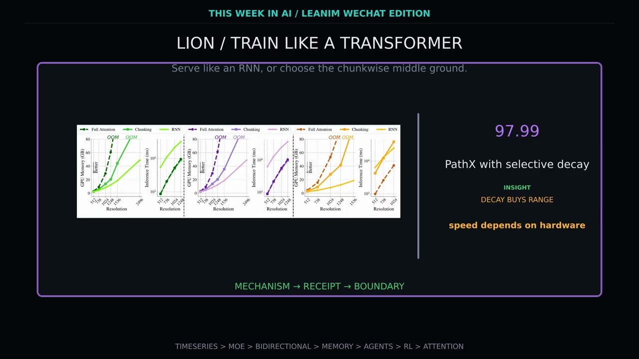
Sequential structures such as DNA sequences, protein chains, and 2D image patches are not inherently directional and gain large representational benefits from processing context forward and backward simultaneously. Standard softmax attention supports bidirectional context but incurs quadratic $\mathcal{O}(N^2)$ memory and compute costs. The LION framework (Linear Bidirectional Transformer Unification) unifies bidirectional linear attention across three mathematically equivalent implementations:

1. **Full Form**: Employs an explicit bidirectional decay mask across the sequence, suitable for parallel training runs. 2. **Recurrent Form**: Runs two decoupled hidden state updates—one processing tokens forward from left to right, and the other backward from right to left—yielding low inference memory footprint. 3. **Chunk Form**: Computes dense parallel matrix operations within isolated sequence chunks while transferring compact state summaries across adjacent chunk boundaries.

A key mechanical issue arises where the two directional passes intersect: the token residing at the immediate scan boundary would be accounted for in both passes. To eliminate this redundancy, LION explicitly subtracts one-half of the diagonal contribution ($\frac{1}{2}\text{diag}$), preventing the central token from being double-counted.

*Claim Boundary*: The practical speedups reported for LION are strictly hardware- and configuration-dependent, relying heavily on batch sequence length, chosen chunk boundaries, and GPU memory architecture.

---

[07:31](https://www.youtube.com/watch?v=ByYH5n0rhW8&t=451s) Falcon: Causally Aligned Fast-Weight Memory

```mermaid flowchart TD accTitle: Falcon Causal Alignment Update Step accDescr: Chronological sequencing showing how key at T-1 predicts value at T before writing residuals back into fast-weight memory.

subgraph Timeline["Causal Timeline Alignment"] T1["Token T-1: Generates Feature φ(k_{T-1})"] T2["Token T Arrives: Reveals True Target Value v_T"] Pred["State Matrix Predicts Value: y_hat_T = W_{T-1} * φ(k_{T-1})"] Res["Compute Residual Error: e_T = v_T - y_hat_T"] Norm["Scale Step by Feature Energy: η / (||φ(k_{T-1})||² + λ)"] Update["Write to Memory: W_T = W_{T-1} + Scaled Residual ⊗ φ(k_{T-1})"] end

T1 --> Pred T2 --> Res Pred --> Res Res --> Norm Norm --> Update ```

Recurrent attention mechanisms are frequently treated as simple storage engines that blindly overwrite previous key-value states with the newest inputs. The Falcon architecture re-examines the causal timeline of fast-weight memory to enforce exact chronological consistency: what features were visible when an outcome materialized?

In standard sequence modeling, token $T-1$ generates the input feature vector $X_T = \phi(K_{T-1})$, but the actual target value $Y_T = V_T$ is revealed only upon observing token $T$. The internal memory matrix $W$ must first predict the current value using the prior key representation; only after the true value arrives can the prediction residual error be identified and written into the weight matrix. While pairing identical time-step keys and values ($K_T, V_T$) technically maintains causal autoregression, it optimizes a misaligned internal objective by ignoring the operational delay of sequential arrival.

To avoid memory saturation, Falcon normalizes its learning update by the incoming feature energy plus a regularization parameter $\lambda$, preventing high-magnitude features from destabilizing stored weights:

- **Falcon-1**: Applies a single scalar update step size across the hidden representation. - **Falcon-2**: Assigns independent learning gains across each value channel. - **Falcon-3**: Averages updates across a sliding window of recent tokens. - **"A" Variants (e.g., Falcon-3A)**: Replace regression error residuals with pure inner-product write mechanisms, explicitly materializing an outer-product update between features and values. - **Empirical Results**: Under matched evaluation protocols, Falcon-1-3 achieves a FineWeb-Edu validation perplexity of $17.1$, while Falcon-3A-3 delivers an $87.2\%$ mean accuracy on variable-length addition benchmarks. - **Boundary**: These findings reflect targeted algorithmic adjustments on specific downstream tasks rather than a blanket replacement for all recurrent attention patterns.

---

[09:26](https://www.youtube.com/watch?v=ByYH5n0rhW8&t=566s) Research Preference Models for Compute-Constrained Agents

```mermaid flowchart TD accTitle: Research Preference Model Pipeline accDescr: Comparison of unexecuted candidate branches via inference-only or agentic sandboxed runs under fixed compute budgets.

subgraph Generation["Branching Ideas"] Idea1["Candidate Branch A (Code Change)"] Idea2["Candidate Branch B (Code Change)"] end

subgraph RPM["Research Preference Model (RPM) Selection Gate"] G1["Inference-Only Mode: Evaluates Task + Search History + Source Diffs"] G2["Agentic Sandbox Mode: Runs Short Pilot Experiments & Inspects Early Traces"] end

subgraph Execution["Targeted Resource Allocation"] H200["Execute Chosen Candidate on Full H200 Run"] end

Idea1 --> RPM Idea2 --> RPM RPM -->|"Selects Branch with Higher Expected Gain"| H200 ```

Autonomous research agents can propose dozens of candidate code modifications, but hardware availability—such as a single NVIDIA H200 GPU bound by a 24-hour run window—precludes training every permutation to convergence. Rather than trying to estimate the exact final metric of a proposed script, a Research Preference Model (RPM) reframes experiment selection as a pairwise ranking problem: given two unexecuted code candidates, which branch deserves allocation of the next compute run?

The model operates across two deployment paradigms: - **Inference-Only RPM**: A frozen language model reads the initial problem specification, historical experiment logs, and proposed source patches to select the more promising candidate. - **Agentic RPM**: The model spins up fast, inexpensive sandbox pilots, inspects initial validation loss slopes and execution traces, and aborts low-performing runs before expending compute on full training jobs.

The system never evaluates against hidden test labels; it serves purely as a resource allocation gate for expensive training loops. Across an evaluation suite spanning 20 benchmark tasks and 10 random seeds, the unguided baseline finishes with a normalized score of $0.684$. Inference-only RPM reaches $0.711$, while agentic RPM attains $0.729$. Because agentic RPM spends initial GPU time on pilot runs, its benchmark curve rises more slowly before pulling ahead. Crucially, both RPM methods match the unguided baseline's 24-hour final score in roughly 15 hours ($14.88$ hours for inference-only, $15.5$ hours for agentic).

The selection advantage—defined as the score difference between chosen candidates and the overall candidate pool—correlates with final task results at approximately $r = 0.55$. However, because per-step win probabilities remain only modestly above $50\%$, RPM should be viewed as structured decision-making under uncertainty rather than an infallible verification oracle.

---

[11:24](https://www.youtube.com/watch?v=ByYH5n0rhW8&t=684s) OPSA: Teacher-Free On-Policy Distillation

```mermaid flowchart TD accTitle: OPSA Teacher Elimination Mechanism accDescr: Elimination of noisy external teacher supervision by penalizing low-log-probability token tails with an entropy-scaled advantage.

subgraph StandardOPD["Standard On-Policy Distillation (Flawed)"] S["Student Rollout Prefix"] --> T["External Large Teacher"] T -->|"Off-Policy Noise (50% Noisy Gradient Supervision)"| G1["Unreliable Token Feedback"] end

subgraph OPSA["OPSA: Internal Policy Reshaping"] P["Model Policy Logits"] --> LowProb["Identify Low Log-Prob Tail Tokens"] LowProb --> Scale["Apply Negative Advantage Scaled by Entropy"] Scale --> Shift["Reallocate Probability Mass back to Head Tokens"] end ```

On-policy distillation (OPD) is conventionally structured around a student model generating token trajectories and an external, higher-capacity teacher scoring every generation step. However, because the initial generation prefix originates from the student, it is inherently off-policy from the perspective of the teacher. This mismatch produces distorted supervision: mathematically correct reasoning paths can receive negative gradient penalties, while incorrect completions are assigned positive rewards. Experiments reveal that across large teacher settings, nearly half of the answer-token supervision signals are noisy. Remarkably, filtering the data into clean-only versus noisy-only splits yields nearly identical student training curves, demonstrating that external teacher guidance is not the primary driver of performance gains.

Investigating which tokens actually shift policy gradients reveals that distillation primarily penalizes tokens with very low log-probabilities. In fact, $29.2\%$ of advantage values are precisely zero, and $51.7\%$ maintain an absolute magnitude below $10^{-4}$.

OPSA (On-Policy Self-Advancement) eliminates the external teacher entirely by directly modifying the student's own token probability tails: - **Tail Penalization**: Low-probability tokens are systematically assigned a negative advantage, pruning unpromising exploration branches. - **Entropy Gating**: The magnitude of this negative advantage is dynamically scaled by local sequence entropy—applying stronger suppression at high-entropy decision forks and weaker adjustments where the policy is already confident. - **Probability Redistribution**: Probability mass stripped from the low-probability tails is returned to head tokens, leaving confident predictions untouched. - **Downstream Impact**: Evaluated on Qwen2.5-Math-7B on the AIME 24 mathematics benchmark, the average score at 32 passes increases from $13.44\%$ to $48.85\%$, confirming that policy self-regularization can outperform external distillation supervision.

[13:18](https://www.youtube.com/watch?v=ByYH5n0rhW8&t=798s) OPSA Wrap-Up: Efficiency and Distribution Shaping

Before moving away from policy optimization, the speaker concludes the empirical case for On-Policy Self-Distillation (OPSA) by examining its efficiency gains and scaling limits. Beyond accuracy jumps, OPSA delivers a substantial leap in coverage and throughput: its `pass@32` rises sharply from 40% to 80%, while training step time drops from On-Policy Distillation's (OPD) 61.2 seconds down to 46.3 seconds. Because the framework eliminates the forward pass of an external teacher model, training becomes noticeably lighter and faster.

At the same time, the speaker issues an important caveat against over-interpreting these benchmarks. Because evaluations topped out at the 9-billion-parameter scale, the mechanism should be understood primarily as "distribution shaping, not proof of new knowledge at every scale." Rather than infusing the model with net-new world facts, OPSA realigns and concentrates the model's existing capabilities by pruning low-confidence exploratory paths.

- **`pass@32` metric**: Surges from 40% up to 80%. - **Step latency**: Falls from 61.2 seconds (OPD) to 46.3 seconds per training step (OPSA). - **Scale boundary**: Verified up to 9B parameters, acting as policy distribution shaping rather than broad multi-scale world knowledge injection.

---

[13:40](https://www.youtube.com/watch?v=ByYH5n0rhW8&t=820s) Sliding-Window Attention vs. Linear Attention: The Missing Baseline

The comparison between full attention, linear attention, and sliding-window attention (SWA) exposes one of the most persistent methodological blind spots in modern architecture research. Full attention grants every single token uninhibited access to the past, but its key-value (KV) cache inflates linearly with context length, leading to prohibitive memory footprints. Linear attention architectures—such as Gated DeltaNet (GDN), Gated Linear Attention (GLA), and RWKV-v6—attempt to solve this by collapsing history into a fixed-size recurrent state. However, this state faces the constant burden of deciding what to retain and what to overwrite, frequently dropping long-range needles in retrieval tasks and demanding roughly 100 million tokens of post-training retrofit.

```mermaid flowchart TD accTitle: SWA vs Linear Attention Mechanisms accDescr: Diagram contrasting sink-aware sliding-window attention with recurrent linear attention states.

subgraph SWA["Sink-Aware Sliding-Window Attention (Zero Post-Training)"] Sinks["First 4 Attention Sinks (Dump unused softmax mass)"] Window["Sliding Window W (Latest 64 or 512 tokens)"] Sinks --- Window SWA_Out["Pretrained Softmax Output (Memory plateaus, throughput flat)"] Window --> SWA_Out end

subgraph Linear["Linearized Retrofits (e.g., Gated DeltaNet)"] InTokens["Incoming Context Stream"] Carry["Learned Finite State Updates & Carry Gate"] InTokens --> Carry RecState["Fixed Recurrent State (Decides overwrite vs keep)"] Carry --> RecState PostTrain["Requires ~100M tokens post-training"] RecState --> PostTrain end ```

The recent sliding-window paper intervened not by designing a fancy new attention kernel, but by insisting on a fair, repaired baseline. Standard sliding-window attention keeps the latest $W$ tokens alongside the first four initial tokens, termed "attention sinks." These sinks are not necessarily semantically meaningful text; rather, they serve as stable numerical dumps where softmax attention can safely park surplus attention mass. Without sinks, an evicted window suffers catastrophic representation collapse the instant initial tokens fall outside the frame. With sinks preserved, a standard pre-trained model needs exactly zero post-training tokens: "The mechanism is humble, a moving local band plus four fixed dots."

When evaluated against this repaired baseline, the narrative surrounding linearized attention shifts dramatically. Prior papers routinely benchmarked their models against *sink-free* SWA—an artificially handicapped baseline destined to collapse. Once sink-aware SWA is restored, it substantially outperforms the linearized field across standard benchmarks:

| Model / Baseline | Average Metric Set 1 | Average Metric Set 2 | Average Metric Set 3 | Post-Training Budget | |:--- |:--- |:--- |:--- |:--- | | **Gated DeltaNet (GDN)** | 56.1 | 48.1 | 55.7 | ~100M tokens | | **Sink-Aware SWA** | **71.6** (+15.5) | **60.9** (+12.8) | **74.9** (+19.2) | **0 tokens** |

Long-context stress tests reinforce the same conclusion: - **4K Single-Needle Retrieval**: SWA with a 512-token window achieves retrieval scores of 19%, 23%, and 23%, while LoLCATs drops to 8.8%, 16.6%, and 5.8%. - **BAbI Long**: SWA achieves 15% accuracy versus 3% for LoLCATs (with full attention anchoring the ceiling around 60%). - **Hardware Profile**: SWA memory usage completely plateaus once the local window fills up, keeping execution throughput essentially flat. - **Scope & Limitations**: The speaker stresses that the goal is not to argue linear attention can never win, but that researchers must first clear a training-free, sink-aware baseline. SWA claimed the highest average score in 9 out of 11 evaluated model configurations, though the study leaves open full-attention hybrids, multimodal models, and specialized agent workflows.

---

[17:19](https://www.youtube.com/watch?v=ByYH5n0rhW8&t=1039s) The Unified Principle: Information Flow Over Brute Force

The speaker unifies all seven papers into a single diagnostic thread, illustrating how each paper triumphs by constraining and routing information paths rather than throwing unguided compute at the problem:

- **TimesFM-3**: Clarifies which variables can legally be visible in future time horizons during multivariate forecasting. - **SMELT**: Asks whether executing a second shared loop computation yields more expressive power than widening network layers under an identical compute budget. - **LION**: Discovers how to preserve bidirectional context processing in linear attention without quadratic memory or double counting. - **Falcon**: Pinpoints precisely which causal examples must update an internal fast-weight memory. - **Research Preference Models (RPM)**: Solves which experimental candidate deserves the next expensive evaluation budget. - **OPSA**: Formulates which uncertain, drifting tokens must receive negative credit during teacher-free on-policy distillation. - **Sliding-Window Attention (SWA)**: Tests whether four fixed attention sinks inside a finite local window are sufficient before undertaking the costly retrofit of an entirely new linear attention kernel.

The underlying lesson for machine learning practitioners is an operational discipline: "First, draw the object, then name the information it can see, then measure the operation that changes it. Only after that should we scale the model or trust the headline." Progress comes from routing signal across variables, recycling compute within matched budgets, and eliminating structural shortcuts that induce false overconfidence—whether that shortcut takes the form of an arbitrary endpoint prior, a noisy distillation teacher, an uncontrolled KV cache, or a flawed benchmark control. As the walkthrough concludes: "A carefully chosen limit can reveal the operation that brute force was hiding. Benchmarks are evidence, not universal laws. Audit the path, then spend the compute."

## Notable quotes > when should we scale a model—and when should we change how information flows? — Xiaol.x

> [00:01](https://www.youtube.com/watch?v=ByYH5n0rhW8&t=1s) Should we add capacity or change which information is allowed to move? — Xiaol.x

> [03:31](https://www.youtube.com/watch?v=ByYH5n0rhW8&t=211s) The scaling curves are fitted across single experimental runs per grid coordinate; they represent observed empirical trends under specific compute budgets rather than universal physical guarantees. — Xiaol.x

> [05:30](https://www.youtube.com/watch?v=ByYH5n0rhW8&t=330s) The practical speedups reported for LION are strictly hardware- and configuration-dependent, relying heavily on batch sequence length, chosen chunk boundaries, and GPU memory architecture. — Xiaol.x

> [13:18](https://www.youtube.com/watch?v=ByYH5n0rhW8&t=798s) distribution shaping, not proof of new knowledge at every scale. — Xiaol.x

> [13:40](https://www.youtube.com/watch?v=ByYH5n0rhW8&t=820s) The mechanism is humble, a moving local band plus four fixed dots. — Xiaol.x

> [17:19](https://www.youtube.com/watch?v=ByYH5n0rhW8&t=1039s) First, draw the object, then name the information it can see, then measure the operation that changes it. Only after that should we scale the model or trust the headline. — Xiaol.x

> [17:19](https://www.youtube.com/watch?v=ByYH5n0rhW8&t=1039s) A carefully chosen limit can reveal the operation that brute force was hiding. Benchmarks are evidence, not universal laws. Audit the path, then spend the compute. — Xiaol.x

> Benchmarks are evidence—not universal laws. Follow the mechanism, inspect the comparison, and keep the claim’s boundary visible. — Xiaol.x

## Mentioned TimesFM-3, SMELT, LION, Falcon, Research Preference Models (RPM), OPSA (On-Policy Self-Advancement), Sliding-Window Attention (SWA), Gated DeltaNet (GDN), Gated Linear Attention (GLA), RWKV-v6, LoLCATs, Vision Mamba, Qwen2.5-Math-7B, Google, NVIDIA H200, GIFT-Eval, ForecastBench, DCLM-Baseline, ImageNet-1K, Long Range Arena: PathX, FineWeb-Edu, AIME 24, BAbI Long

## Video description Seven recent AI papers, explained through one practical question: when should we scale a model—and when should we change how information flows?

This professional, visual lesson covers forecasting, looped Transformers, bidirectional linear attention, fast-weight memory, AI research agents, teacher-free policy optimization, and sliding-window attention.

You’ll learn:

- How TimesFM-3 combines temporal and cross-variable information - Whether looped Transformers remain efficient under matched budgets - How LION enables bidirectional processing without quadratic memory - Why causal alignment matters for fast-weight attention - How preference models allocate expensive research experiments - Why OPSA can improve Qwen models without an external teacher - Why attention sinks make SWA a much stronger baseline - Why GDN leads the tested linearized methods, yet still trails sink-aware SWA in the reported averages - What the SWA paper actually contributes: a fair baseline comparison, not a new attention kernel

Chapters

00:00 The central question: capacity or information flow? 00:59 Seven papers, one evaluation framework 01:52 TimesFM-3: multivariate forecasting 03:31 SMELT: looped Transformers under equal budgets 05:30 LION: bidirectional linear attention 07:31 Falcon: causally aligned fast-weight memory 09:26 Research Preference Models 11:24 OPSA: does on-policy distillation need a teacher? 13:39 SWA vs linear attention, including GDN 17:19 The shared principle 18:11 Final takeaways

Papers

TimesFM-3 https://research.google/blog/timesfm-3-a-zero-shot-foundation-model-for-multivariate-forecasting/

SMELT https://arxiv.org/abs/2609.01343

LION https://arxiv.org/abs/2502.16249

Fast-Weight Attention https://www.alphaxiv.org/abs/2608.27763

AI Research Preference Models https://arxiv.org/abs/2608.13940

OPSA https://huggingface.co/papers/2608.31046

Sliding-Window Attention vs Linear Attention https://arxiv.org/abs/2608.28444

Benchmarks are evidence—not universal laws. Follow the mechanism, inspect the comparison, and keep the claim’s boundary visible.

#AIResearch #MachineLearning #LLM #LinearAttention #TimeSeries #Qwen #ResearchPapers

[Source](https://www.youtube.com/watch?v=ByYH5n0rhW8)

中文简报

信息流胜过蛮力扩增：解析7篇重要AI论文该视频评估了针对预测跨度、算力受限的研究闭环以及KV缓存内存激增等实际约束提出的七项架构方案。所考察的论文并未依赖蛮力扩展参数，而是证明了性能提升源自对信息传递路径的重构——例如TimesFM-3中的跨变量路由、SMELT中的计算复用、Falcon中的因果权重对齐，以及OPSA中无教师模型的尾部熵剪枝。关键在于，讨论强调了实证研究的严谨性，展示了合理的基准调整（例如在滑动窗口注意力中恢复attention sink）往往能够超越代价高昂的线性注意力改造，且无需额外的后训练。感知Sink的滑动窗口注意力（SWA）揭示了线性注意力研究中的一个重大评估盲区；在完全无需后者约1亿token后训练的情况下，其在基准测试上的平均表现高出Gated DeltaNet等改造方案达两位数百分比。 (13:40) OPSA表明在线策略蒸馏无需外部教师模型；直接惩罚低概率token尾部使单步训练时间从61.2秒缩短至46.3秒，同时在数学推理任务上将pass@32从40%翻倍提升至80%。 (13:18) 在SMELT框架下于严格匹配的FLOP、KV缓存和参数预算内进行评估的循环Transformer，通过结合缩放残差重复访问中间MoE层，在10^21 FLOPs下节省了14.7%至18.0%的计算量。 (3:31) 研究偏好模型（RPM）将实验优先级划定为成对排序而非结果预测，使算力受限的自主智能体能够在不到15小时内达到24小时基线基准测试的成绩。 (9:26)

Reading summary

Rather than relying on brute-force parameter scaling, recent architectural advances succeed by reshaping information flow—enforcing causal boundaries, recycling compute, and establishing rigorous baseline controls. Aligning Causal and Directional Information Flow (1:52) Standard sequence models often blur temporal boundaries or incur prohibitive costs when expanding context. In multivariate time-series forecasting, TimesFM-3 separates these dynamics by applying strictly causal attention across time while maintaining bidirectional attention across concurrent covariates like weather or promotions. Slicing continuous data into patches of 32 and masking future targets contiguously, the 330-million-parameter model forecasts multi-horizon quantiles (P10 through P90) in parallel, attaining leading relative rankings across GIFT-Eval and ForecastBench. In recurrent sequence modeling, directional constraints require precise synchronization. LION unifies bidirectional linear attention across full, chunk, and recurrent modes, eliminating token double-counting at scan boundaries by explicitly subtracting half the diagonal contribution; on Long Range Arena's PathX, its selective decay achieves 97.99% accuracy where decay-free variants fail. Similarly, Falcon realigns recurrent fast-weight updates with sequence causality: because token T-1 generates key features while token T reveals the actual target value, Falcon computes prediction residuals against the prior state before writing normalized updates into memory, reaching a FineWeb-Edu validation perplexity of 17.1. Recycling Compute and Gating Candidate Experiments (3:31) When compute envelopes are strictly constrained, restructuring internal execution paths outperforms widening network layers. The SMELT framework tests looped Transformers under matched token, parameter, and KV-cache budgets by routing tokens through the middle 50% of layers twice with second-pass residuals scaled by 0.5. At 10^21 FLOPs, SMELT yields 14.7% to 18.0% compute savings to match baseline loss, dropping 200-million-parameter validation loss from 1.9445 to 1.9257 and lifting DCLM accuracy from 24.92% to 27.57%. At the macro level of automated experimentation, Research Preference Models (RPM) apply compute efficiency to candidate selection. Instead of training every code proposal to convergence on scarce hardware, RPM ranks unexecuted ideas via frozen LLM evaluation or brief agentic sandbox runs. Evaluated across 20 benchmark tasks, RPM methods reached the 24-hour baseline performance of unguided search in roughly 15 hours, achieving normalized scores of 0.711 (inference-only) and 0.729 (agentic) compared to the unguided 0.684 baseline. Teacher-Free Distillation via Token Tail Shaping (11:24) Conventional on-policy distillation pairs a student model with a larger teacher, but because student rollouts are off-policy from the teacher's perspective, approximately half of the resulting supervisory gradients contain noisy feedback. Analysis reveals that performance gains stem primarily from suppressing low-probability token tails, with over half of advantage values hovering below 10^-4 or landing at zero. On-Policy Self-Advancement (OPSA) discards the external teacher entirely, directly penalizing the student's own low-probability tails with a negative advantage scaled by local sequence entropy. Stripped probability mass is redistributed back to confident head tokens. On Qwen2.5-Math-7B, AIME 24 accuracy at 32 passes rose from 13.44% to 48.85%, while training step time decreased from 61.2 seconds under teacher distillation to 46.3 seconds. Verified up to 9 billion parameters, OPSA acts as distribution regularization rather than an injection of new factual knowledge. Attention Sinks and Fair Long-Context Baselines (13:40) Evaluating novel architectures requires measuring against properly configured baselines. Linearized attention models—such as Gated DeltaNet, GLA, and RWKV-v6—compress context into fixed states to avoid KV-cache memory explosions, but they often require around 100 million post-training tokens and struggle with long-range retrieval. Investigations reveal that prior work demonstrated advantages largely by comparing against sink-free sliding-window attention (SWA), which suffers numerical collapse once initial tokens exit the window. When standard SWA retains the first four 'attention sink' tokens alongside a local window of 64 or 512 tokens, it requires zero post-training tokens and outperforms linearized retrofits across benchmark suites (achieving scores such as 71.6, 60.9, and 74.9 compared to Gated DeltaNet's 56.1, 48.1, and 55.7). On 4K single-needle retrieval, 512-token sink-aware SWA recovered 19% to 23% accuracy, whereas LoLCATs dropped to 5.8% to 16.6%, demonstrating that simple local masking with numerical sinks often surpasses complex architectural replacements. Across these investigations, meaningful performance improvements stemmed from mapping visible information pathways, enforcing causal synchronization, and testing against uncompromised controls rather than expanding raw capacity. The collective findings caution that empirical benchmarks represent situated evidence within specific compute regimes rather than universal laws, making path auditing essential prior to scaling.

Source quotes

Xiaol.x: when should we scale a model—and when should we change how information flows? [0:01] Xiaol.x: Should we add capacity or change which information is allowed to move? [3:31] Xiaol.x: The scaling curves are fitted across single experimental runs per grid coordinate; they represent observed empirical trends under specific compute budgets rather than universal physical guarantees. [5:30] Xiaol.x: The practical speedups reported for LION are strictly hardware- and configuration-dependent, relying heavily on batch sequence length, chosen chunk boundaries, and GPU memory architecture. [13:18] Xiaol.x: distribution shaping, not proof of new knowledge at every scale. [13:40] Xiaol.x: The mechanism is humble, a moving local band plus four fixed dots. [17:19] Xiaol.x: First, draw the object, then name the information it can see, then measure the operation that changes it. Only after that should we scale the model or trust the headline. [17:19] Xiaol.x: A carefully chosen limit can reveal the operation that brute force was hiding. Benchmarks are evidence, not universal laws. Audit the path, then spend the compute. Xiaol.x: Benchmarks are evidence—not universal laws. Follow the mechanism, inspect the comparison, and keep the claim’s boundary visible.

Original transcript

[0:01] Before we name a model, picture three [0:03] constraints. [0:05] A forecast sees yesterday's sales, but [0:08] can miss tomorrow's promotion. [0:11] A research run has 15 plausible ideas, [0:15] but one expensive experiment. And [0:17] attention cash grows until memory, not [0:20] accuracy sets the limit. [0:22] These are the three cards on the board: [0:24] forecast, experiment, context. The [0:27] question is not automatically make the [0:32] model bigger. [0:33] It is, should we add capacity or change [0:37] which information is allowed to move? [0:39] This week's seven papers answer that [0:41] question [0:43] um in different places. Some route [0:45] information across variables or [0:47] directions. [0:48] Some reuse a computation, some remove a [0:50] shortcut. We will keep one discipline [0:52] throughout. Draw the path first, then [0:55] show its measurement, then say where the [0:57] claim stops. [0:58] Now, turn the pressures into a map. The [1:00] first row holds times FM, three, smelt, [1:03] lion, and falcon. The second row holds [1:06] RPM, ops and swa. Read every card in the [1:09] same three steps. [1:11] Um First, what information path changed? [1:15] Variables, a shared loop, two [1:17] directions, a causal right, a selection [1:20] gate, token tails, or a finite window. [1:23] Second, [1:25] what receipt did the authors report? A [1:28] forecast ranking, matched budget loss, [1:32] accuracy, perplexity, selection score, [1:35] training curve, or retrieval recovery. [1:38] Third, what boundary keeps the result [1:40] honest? This map prevents a headline [1:44] from floating free of its mechanism. It [1:47] also tells you what to watch for as each [1:49] paper gets its own board. [1:52] Start with an ice cream shop. The red [1:55] line is yesterday's sales. The blue line [1:58] adds related products, weather, and a [2:01] promotion calendar. If a sale is [2:05] scheduled tomorrow, that future covaria [2:08] is already known even though tomorrow's [2:10] target is not. Uh Times FM 3 is a 330 [2:16] million parameter foundation model [2:18] trained on more than 1 trillion time [2:20] points. It cuts continuous data into [2:23] patches of 32, normalizes each series [2:26] independently, and predicts multiple [2:28] targets together. The important teaching [2:31] move is to separate what is hidden from [2:33] what is legitimately known. A mask [2:35] covers future sales, but the promotion [2:38] signal stays visible. [2:40] Now, watch the attention pattern. [2:43] Along time, attention is causal. [2:46] A token cannot look into a future [2:48] target. Across variables, attention is [2:50] full. Sales can read weather or a [2:53] neighboring product at the same time. [2:55] The model alternates those two views, [2:57] then masks the future target patches in [2:59] one contiguous block. It fills the whole [3:02] forecast horizon in parallel instead of [3:04] making one fragile guess after another. [3:07] Uh for every future point, it emits nine [3:10] quantiles [3:12] from P10 to P90. So, the answer is a [3:15] range, not just a dot. Across Gift Evil, [3:19] FEB bench, and Time Times FM, 3 has the [3:22] best average ranking among the compared [3:25] foundation models. That is a ranking [3:27] claim, not a promise to win every data [3:30] set. [3:32] A looped transformer reuses a block, so [3:35] the diagram looks economical. But, reuse [3:38] also means extra computation, and a [3:40] larger effective depth can require a [3:42] smaller width. Uh Smell asked the fair [3:45] question, if we match per token flops, [3:48] total non-embedding parameters, and KB [3:51] cache, does looping still help? The [3:53] recipe is a sparse mixture of experts [3:57] decoder with the middle half of the [4:00] layers visited twice. Residual updates [4:03] inside the second visit are scaled by [4:05] one over the number of visits, here 1/2, [4:08] to keep the stream stable. The [4:10] comparison is not big model versus small [4:12] model. It is the same budget with a [4:14] different allocation of depth and width. [4:17] The scaling law board makes the result [4:20] concrete. Smelt fits loss as a function [4:23] of compute, sparsity, and data, then [4:26] compares the compute needed to reach the [4:28] same loss. Its fitted exponent is 0.25 [4:34] versus 0.237 [4:36] for the baseline, a modestly steeper [4:39] frontier. At [4:42] 10 to the 21st flops, the reported [4:45] compute saving is about 14.7 to 18% [4:49] in the match 200 million scale ablation [4:54] validation loss moves from [4:56] 1.9445 [4:58] to 1.9257 [5:02] and DCLM core moves from 24.92 [5:07] to 27.57. [5:09] Um the mechanism evidence is also [5:12] interesting. The second visit reuses [5:15] similar experts, changes values more [5:17] than queries and keys, and reduces [5:18] attention paid to the initial sync [5:20] tokens. The paper has one run per grid [5:24] point, so treat the frontier as evidence [5:26] of a trend, not a guarantee. [5:30] Many sequences are not naturally left to [5:33] right. DNA, proteins, and image patches [5:36] benefit from seeing both directions. [5:39] Full softmax attention gives that view, [5:42] but builds a quadratic interaction. Lion [5:46] or linear bidirectional transformer [5:49] unification writes the same idea in [5:52] three equivalent forms. The full form [5:55] uses a bidirectional decay mask. The [5:58] recurrent form runs one state forward [6:01] and one backward. The chunk form does [6:04] matrix work inside a chunk and carries a [6:08] compact state across chunk boundaries. [6:11] There is a small trap. The token at the [6:14] meeting point belongs to both scans. [6:17] LION subtracts one half of the diagonal [6:20] contribution so the current token is not [6:22] counted twice. [6:24] The visual payoff is a choice of routes. [6:27] Full linear attention is fast to train [6:30] but materializes more interaction. [6:32] The bidirectional recurrent route is [6:35] memory light at inference. Chunking sits [6:38] between them. [6:40] More parallel work inside each block, [6:43] fewer serial state transfers than a pure [6:46] scan. On ImageNet 1K LION-D with [6:51] multi-scan reaches 79.9% [6:54] for the small model and 80.2% for the [6:57] base model. While Vision Mamba is faster [7:02] only under a different and much heavier [7:07] training cost. On long range arena [7:10] selective decay reaches 97.99 [7:14] on PathX. [7:16] The no decay LIT variant fails the long [7:19] range test. The paper's honest message [7:22] is conditional. The decay structure [7:24] matters and the claimed speed up depends [7:27] on sequence length, chunk size, and [7:29] hardware. [7:31] A recurrent attention state is often [7:33] described as if it simply stores the [7:35] latest key and value. Falcon asks us to [7:38] slow down and draw the causal timeline. [7:41] Token T minus one produces a feature. [7:44] Token T reveals the value we want to [7:47] predict. [7:49] Um only then does the fast memory update [7:52] and the updated state is read for the [7:54] next prediction. In symbols, the local [7:56] pair is X sub T equals 5 K sub T minus 1 [8:01] and Y sub T equals V sub T. The tempting [8:05] same step pair is still causal, but it [8:06] optimizes a different internal [8:08] objective. Alignment is the contribution [8:11] identify what the learner could actually [8:12] see when the target arrived. [8:15] Now put the state matrix on the board. [8:17] It predicts a value. The revealed value [8:20] exposes a residual and the update writes [8:24] feature times residual back into the [8:26] matrix. A normalized step size divides [8:30] by feature energy plus regularization. [8:35] So, allowed feature does not cause an [8:37] uncontrolled right. [8:39] Falcon 1 uses one scalar gain. [8:43] Falcon 2 gives each value channel its [8:47] own gain. Falcon 3 averages a sliding [8:50] window of recent examples. [8:52] The A variance replace regression [8:54] residuals with an inner product right [8:56] making the feature value outer product [8:58] explicit. In the reported matched [9:01] experiments, Falcon 1 3 reaches fine web [9:05] edge you perplexity 17.1 [9:08] and Falcon 3 A 3 reaches 87.2 [9:14] mean accuracy on variable length [9:16] addition. Those are those are selected [9:20] variants and task specific receipts, not [9:23] a universal win. [9:26] Research agents can generate many [9:28] plausible code changes, but one H200 [9:32] cannot fully train all of them inside a [9:35] 24-hour run. [9:37] A research preference model changes the [9:39] question. It does not predict [9:43] the exact final score. [9:45] It compares two unexecuted children and [9:49] chooses which branch deserves the next [9:51] expensive experiment. In the inference [9:54] only version of frozen language model [9:56] reads the task, the search history, and [9:59] the candidate code. In the agentic [10:02] version, it can run small pilots in a [10:05] sandbox, receive feedback, and stop [10:08] before the real budget is gone. [10:10] The live system never sees hidden test [10:13] labels. [10:14] It is a decision gate that reallocates [10:17] verification, not an oracle that makes [10:20] verification free. [10:22] The results curve separates early and [10:24] late behavior. [10:26] With no RPM, the average normalized [10:29] score finishes at 0.684. [10:33] Inference only reaches 0.711, [10:36] and agentic reaches 0.729, [10:40] with the agentic curve rising more [10:42] slowly because it spends time on pilots. [10:45] Both guided methods match the baseline's [10:48] 24-hour score in roughly 15 hours. [10:51] 14.8 8 hours and 15.5 hours. Selection [10:56] advantage, the chosen child's score [10:58] above the average child's score [11:01] correlates with the final result at [11:03] about R equals 0.55. [11:07] The benchmark has 20 public tasks and 10 [11:11] seeds, and the improvement probabilities [11:14] are modestly above 1/2. So, the durable [11:17] lesson is budget allocation under [11:19] uncertainty with a measured but not [11:22] magical gain. [11:24] On policy distillation sounds like a [11:26] clean division of labor. [11:28] The student samples a trajectory, and a [11:30] stronger teacher scores every token, but [11:34] the prefix came from the student, so it [11:37] is off-policy for the teacher. A correct [11:40] answer can receive negative credit, an [11:43] incorrect answer can receive positive [11:45] credit. In the largest teacher [11:47] condition, the paper reports noise on [11:49] roughly half of answer token [11:51] supervision. The surprise is stronger [11:55] standard OPD, clean only OPD, and noisy [11:58] only OPD reach comparable training [12:01] curves. If noisy supervision still [12:04] improves the student, perhaps the [12:06] teacher is not the main source of the [12:08] gain. We need to inspect which tokens [12:11] actually move the gradient. The signal [12:14] concentrates in low log probability [12:16] tokens. [12:18] Nearly 29.2% [12:20] of advantages are exactly zero, and [12:23] 51.7% [12:25] have magnitude at most 10 to the minus [12:27] four. Opsa keeps the useful direction [12:31] and removes the external teacher. At the [12:34] lowest log positions, it applies a [12:36] negative advantage, an entropy term [12:38] makes that negative signal stronger at [12:41] high entropy forks, and gentler where [12:44] the model is already confident. In a [12:47] four-case drawing, a tail token loses [12:49] probability, head tokens receive the [12:51] returned mass, and confident head [12:54] positions outside the selected tail stay [12:56] untouched. On Qwen 3 1 7B, [13:04] AIME [13:06] 2 4, [13:08] average at 32 rises from 13.44 [13:15] to 48.85, [13:18] while pass at 32 rises from 40 to 80. [13:23] Training step time drops from OPD's 61.2 [13:27] seconds to Opsa's 46.3 seconds. [13:31] Um [13:32] the tests reach 9B, so this is [13:34] distribution shaping, not proof of new [13:36] knowledge at every scale. [13:40] Full attention gives every token [13:43] access to the past, but its KV cache [13:46] grows with context. Linear attention [13:48] keeps a fixed recurrent state, yet that [13:50] state must decide what to overwrite and [13:53] may lose a long needle. The sliding [13:55] window paper asked for a fair baseline. [13:58] Sliding window attention keeps the [13:59] latest W tokens and also keeps the first [14:02] four attention sinks. Those sinks are [14:04] not necessarily meaningful content. They [14:08] are stable places where the softmax can [14:10] put unused attention mass. Without them, [14:14] a window can catastrophically degrade [14:17] after the first tokens slide away. [14:20] With them, the pre-trained model needs [14:22] no post-training. The mechanism is [14:25] humble, a moving local band plus four [14:28] fixed dots. [14:30] Here is the [14:32] comparison people often skip. Gated [14:35] DeltaNet or GDN, GLA, and QRWK V6 [14:41] replace softmax attention with learned [14:44] finite state updates. [14:46] GDN adds an explicit carry gate. [14:50] Its state decides both what to overwrite [14:54] and how much history to keep. These are [14:56] serious linearized retrofits, but they [14:59] need post-training and the state must [15:02] learn what not to forget. SWA is much [15:05] simpler. Keep the original pre-trained [15:07] softmax attention, restrict it to the [15:10] latest 64 tokens, and always keep four [15:14] fixed attention sinks. Zero [15:17] post-training tokens. The important [15:19] novelty is not a new mask. Sink aware [15:22] SWA was already known. The novelty is [15:26] the missing comparison. Earlier linear [15:29] attention work often compared against [15:31] sink free SWA, a baseline that collapses [15:34] when the first sync tokens leave the [15:35] window. Once that control is repaired, [15:40] the interpretation changes. In the [15:42] modern model appendix, SWA reaches [15:46] average scores of 71.6, [15:50] 60.9, [15:51] and 74.9, [15:54] while GDN reaches 56.1, [15:57] 48.1, [15:59] and [16:01] 55.7 [16:04] after roughly 100 million post training [16:09] tokens. GDN is the strongest of these [16:13] linearized rows, but SWA is still ahead [16:16] by 15.5, [16:17] 12.8, and 19.2 points. The long context [16:21] receipt points the same way. At 4K on [16:25] single needle retrieval, [16:27] SWA with a 512 token window scores 19, [16:31] 23, and 23%, while low cats falls to [16:34] 8.8, 16.6, and 5.8. On BABI [16:39] long, SWA reaches 15% against 3% for low [16:43] cats, while full attention remains [16:46] around 60%. [16:48] The hardware curves explain the system's [16:50] trade-off. SWA memory plateaus once the [16:53] window is full and throughput stays [16:55] nearly flat. So, the claim is not that [16:58] linear attention can never win. The [17:01] claim is that a strong fair training [17:03] free baseline must be beaten first. SWA [17:07] wins the average in nine of 11 model [17:09] cases, not all of them, and the paper [17:12] does not evaluate every full attention [17:14] hybrid, multimodal, or agentic workload. [17:19] Let's put all seven mechanisms in one [17:22] line. Times FM three asks which [17:25] variables can legally be visible in the [17:28] future. Smell asks whether a second [17:32] shared computation is worth more than [17:34] extra width under equal budgets. Lion [17:38] asks how to preserve two directions [17:41] without double counting. Falcon asks [17:44] which causal example updates a fast [17:47] memory. [17:48] RPM asks which candidate gets the next [17:51] expensive measurement. OPSA asks which [17:54] uncertain tokens deserve negative [17:55] credit. SWA asks whether four sinks in a [17:59] finite window are enough before we [18:01] retrofit a new attention kernel. In [18:04] every case, the paper earns its claim by [18:06] exposing an information path and [18:08] attaching a receipt to it. [18:11] The professional habit is simple. First, [18:13] draw the object, then name the [18:15] information it can see, then measure the [18:18] operation that changes it. Only after [18:20] that should we scale the model or trust [18:22] the headline. Route useful information [18:26] across variables or directions. [18:28] Reuse computation when the budget is [18:30] matched. Remove the shortcut that [18:33] creates confident errors, [18:36] whether it is an endpoint prior, a noisy [18:39] teacher, a growing cash, or an unfair [18:42] baseline. These papers do not prove that [18:46] less is always more. They show something [18:48] more useful. A carefully chosen limit [18:51] can reveal the operation that brute [18:53] force was hiding. Benchmarks are [18:55] evidence, not universal laws. Audit the [18:58] path, then spend the compute.