LeCun Team Finds Sparse Latents Lift World Model Planning by 57 Points
Xiaol.x
Enforcing exact zeros in latent representations linearizes physical transitions across dynamic regimes, allowing compact three-million-parameter predictors to succeed where standard dense representations fail.
AI-assisted summary of LpWM: A Case for Sparse Representations in World Models — original source. Check the original for full context.
Source published:
Key ideas
- Yann LeCun's group introduces LpWM, showing that replacing standard Gaussian latent targets in JEPA world models with rectified Laplace distributions yields 30–65% exact zeros and drastically simplifies the learned dynamics. (0:00)
- On the PushT benchmark, intermediate-capacity predictors using sparse latents outperform dense baselines by up to 57 percentage points, with a compact 3M-parameter MLP ∘ LTI predictor achieving ~70% planning success on sparse codes versus ~7% on dense ones. (6:03)
- Linear probes confirm a mechanistic phenomenon termed 'mode factoring': the latent vector's binary zero-support decodes discrete physical force regimes with 97% accuracy, while continuous coordinate magnitudes encode position within each regime. (9:11)
- While vanilla frame-level sparsity primarily tracks end-effector motion (r = 0.87), introducing an auxiliary temporal Jaccard loss penalizing support flips successfully realigns the zero pattern to track physical contact (r = 0.61) without degrading planning performance. (12:27)
- The performance advantage of sparse representations is restricted to intermediate predictor capacities; when scaled up to high-capacity Diffusion Transformers (DiT), sparse and dense representations achieve identical performance. (13:34)
Detailed notes
## Background Published on YouTube by Xiaol.x on September 11, 2026, this video presents Episode 02 of the podcast 'Loop State'. The episode features hosts Mara and Theo breaking down an August 2026 paper from Yann LeCun's research group (Kuang et al.) that challenges standard Gaussian latent geometry in JEPA world models in favor of sparse representations.
## TL;DR The hosts examine the paper 'LpWM: A Case for Sparse Representations in World Models', which shows that enforcing exact zeros in latent representations makes environment dynamics dramatically simpler to learn. Theoretical intuition rooted in one-hot state partitions motivates RDMReg, a regularizer steering features toward a rectified Laplace distribution to produce 30–65% exact zeros without codebooks. On the PushT benchmark, sparse latents allow intermediate, low-capacity predictors (such as an MLP over linear dynamics) to outperform dense counterparts by up to 57 percentage points, while both representations tie at the deep transformer level. Analysis on the Piecewise and OGBench-Cube benchmarks reveals that active coordinate supports cleanly factor physical modes, though tracking physical contact requires an auxiliary temporal Jaccard loss.
## Atmosphere & style The discussion carries a lively, intellectually curious podcast dynamic where Mara and Theo bounce technical ideas off each other with sharp clarity and approachable analogies. It moves from playful conceptual thought experiments—like calling one-hot physics a lookup table in a linear algebra costume—into precise mathematical and empirical deconstruction. The tone is enthusiastic yet refreshingly skeptical, celebrating the efficiency gains of sparse world models while meticulously probing empirical limitations, missing baselines, and theoretical caveats.
## Bulletin - [00:00](https://www.youtube.com/watch?v=FVpfCJfV110&t=0s) Yann LeCun's group introduces LpWM, showing that replacing standard Gaussian latent targets in JEPA world models with rectified Laplace distributions yields 30–65% exact zeros and drastically simplifies the learned dynamics. - [06:03](https://www.youtube.com/watch?v=FVpfCJfV110&t=363s) On the PushT benchmark, intermediate-capacity predictors using sparse latents outperform dense baselines by up to 57 percentage points, with a compact 3M-parameter MLP ∘ LTI predictor achieving ~70% planning success on sparse codes versus ~7% on dense ones. - [09:11](https://www.youtube.com/watch?v=FVpfCJfV110&t=551s) Linear probes confirm a mechanistic phenomenon termed 'mode factoring': the latent vector's binary zero-support decodes discrete physical force regimes with 97% accuracy, while continuous coordinate magnitudes encode position within each regime. - [12:27](https://www.youtube.com/watch?v=FVpfCJfV110&t=747s) While vanilla frame-level sparsity primarily tracks end-effector motion (r = 0.87), introducing an auxiliary temporal Jaccard loss penalizing support flips successfully realigns the zero pattern to track physical contact (r = 0.61) without degrading planning performance. - [13:34](https://www.youtube.com/watch?v=FVpfCJfV110&t=814s) The performance advantage of sparse representations is restricted to intermediate predictor capacities; when scaled up to high-capacity Diffusion Transformers (DiT), sparse and dense representations achieve identical performance.
## Key takeaways - [00:00](https://www.youtube.com/watch?v=FVpfCJfV110&t=0s) Conventional JEPA world models enforce dense, maximum-entropy Gaussian latents to avoid representation collapse, inadvertently making downstream dynamics unnecessarily complex to learn. - [01:21](https://www.youtube.com/watch?v=FVpfCJfV110&t=81s) JEPA world models conduct planning entirely in abstract latent space without decoding pixels, using predictors as latent physics engines combined with the Cross-Entropy Method. - [02:51](https://www.youtube.com/watch?v=FVpfCJfV110&t=171s) Proposition 1 proves that one-hot latent codes linearize any Lipschitz continuous dynamic system into state-transition permutation matrices, though doing so exactly requires exponentially many dimensions. - [04:30](https://www.youtube.com/watch?v=FVpfCJfV110&t=270s) LpWM relaxes one-hot coding into distributed continuous sparsity using RDMReg, matching 1D random batch projections against a rectified Laplace distribution to force 30% to 65% of coordinates to exact zero. - [04:30](https://www.youtube.com/watch?v=FVpfCJfV110&t=270s) To maintain exact zeros while preserving gradient flow during backpropagation, LpWM's projector uses a standard ReLU forward pass combined with a GELU gradient on the backward pass. - [06:03](https://www.youtube.com/watch?v=FVpfCJfV110&t=363s) The authors establish a predictor complexity ladder spanning from lightweight 3M-to-34M parameter linear models up to 822M-parameter Diffusion Transformers to quantitatively benchmark dynamics complexity. - [06:03](https://www.youtube.com/watch?v=FVpfCJfV110&t=363s) On the PushT benchmark, sparse LpWM outperforms dense LeWM by 24 to 57 points across intermediate predictor rungs like MLP ∘ LTI and by 36 to 45 points on MLP ∘ LTV. - [06:03](https://www.youtube.com/watch?v=FVpfCJfV110&t=363s) Both sparse and dense representations fail completely on single-step linear predictors (LTI(1)) and tie at top-tier Diffusion Transformers, locating the entire sparse advantage within intermediate model capacities. - [09:11](https://www.youtube.com/watch?v=FVpfCJfV110&t=551s) Sparse representations maintain their performance advantage over covariance-penalized VICReg baselines, outperforming VICReg even at the deep transformer tier. - [09:11](https://www.youtube.com/watch?v=FVpfCJfV110&t=551s) In a piecewise-affine room, latent binary supports capture discrete dynamical zones with 97% accuracy even when visual zone boundaries are completely absent, proving sensitivity to physical dynamics over visual textures. - [12:27](https://www.youtube.com/watch?v=FVpfCJfV110&t=747s) Vanilla marginal RDMReg possesses no temporal awareness, causing the zero support pattern out-of-the-box to correlate strongly with arm motion (r = 0.87) rather than physical contact (r = 0.05). - [12:27](https://www.youtube.com/watch?v=FVpfCJfV110&t=747s) An auxiliary temporal Jaccard regularization penalizes support changes across consecutive frames, raising physical contact correlation to 0.61 and cube motion correlation to 0.80 on OGBench-Cube. - [13:34](https://www.youtube.com/watch?v=FVpfCJfV110&t=814s) The empirical implementation operates far from the theoretical one-hot ideal, retaining 30% to 65% active coordinates rather than a strict single active dimension. - [13:34](https://www.youtube.com/watch?v=FVpfCJfV110&t=814s) The empirical study is limited to four simulated planar environments, uses a single training seed with three evaluation seeds, and omits direct empirical comparisons to discrete categorical latents like DreamerV2. - [15:06](https://www.youtube.com/watch?v=FVpfCJfV110&t=906s) LpWM challenges default self-supervised learning assumptions, framing latent geometry as an intentional design variable that can reduce the compute requirements of world model predictors.
## Detailed walkthrough ### [00:00](https://www.youtube.com/watch?v=FVpfCJfV110&t=0s) Rethinking the Gaussian Latent in World Models
Hosts Mara and Theo kick off the second episode of *Loop State* by diving into an August 2026 paper from Yann LeCun's research group: *"LpWM: A Case for Sparse Representations in World Models"* by Kuang et al. Mara introduces the core premise as a fundamental question she had never thought to ask: why does practically every self-supervised world model push its internal representations toward a dense Gaussian blob? Models like LeWM and VICReg enforce dense geometries by design, but the authors pitch a provocative alternative. Dense representations might simply be the wrong shape.
The core thesis of the paper is not just an aesthetic critique, but a functional one: if latent codes are made sparse—meaning a substantial fraction of their coordinates sit at exact zeros—the underlying dynamics that the model must learn become far simpler. In fact, they become so simple that a nearly linear predictor can successfully plan actions where a dense latent representation would demand an expressive, compute-heavy transformer. The headline finding highlights this drastic difference: on the PushT manipulation task, sparse codes beat dense ones by up to 57 percentage points in planning success at intermediate predictor capacity.
- Paper: *"LpWM: A Case for Sparse Representations in World Models"* (Kuang, Dagade, Le Lidec, Maes, Balestriero, LeCun; August 2026). - Headline result: Up to a 57-point improvement in closed-loop planning success over dense representations when using intermediate-capacity predictors.
[01:21](https://www.youtube.com/watch?v=FVpfCJfV110&t=81s) How JEPA Predicts Without Pixels
To unpack why representations matter, Theo breaks down the machinery of a Joint Embedding Predictive Architecture (JEPA) for listeners who have heard the acronym but never opened the foundational papers. A JEPA world model consists of three core components: an encoder $F$ that maps an observation image into a latent vector $z$, a predictor $G$ that takes the current latent $z_t$ alongside an action $a_t$ to forecast the next latent state $\hat{z}_{t+1}$, and a loss function measuring the distance between $\hat{z}_{t+1}$ and the encoded ground-truth target frame $z_{t+1}$. Because the model predicts strictly within its abstract latent space and never decodes images back into pixels, it bypasses the massive overhead of generative pixel modeling.
```mermaid flowchart LR accTitle: JEPA World Model Architecture accDescr: Visual flowchart tracing the JEPA pipeline from observations through latent encoding, prediction, and loss computation against target frames. subgraph Input["Observations"] O_t["Image (t)"] O_next["Image (t+1)"] end subgraph Encoding["Encoder F"] O_t --> Z_t["Latent z_t"] O_next --> Z_next["Latent z_{t+1}"] end subgraph Dynamics["Predictor G"] Z_t --> G_pred{"Predictor G"} A_t["Action a_t"] --> G_pred G_pred --> Z_hat["Predicted ẑ_{t+1}"] end subgraph Objective["Latent Loss"] Z_hat -.-> Loss(["Distance Loss"]) Z_next -.-> Loss end ```
However, predicting directly in latent space introduces a critical failure mode: representation collapse. Without constraints, the encoder can trivially minimize loss by outputting an identical constant vector for every frame, yielding perfect but useless predictions. To prevent this, architects use regularization terms to force latents toward high-entropy distributions: - **LeWM** applies SIGReg to align latents with an isotropic Gaussian. - **VICReg** penalizes covariance to drive the variance-covariance matrix toward the identity.
Because both targets are maximum-entropy distributions, they guarantee dense representations where every single coordinate is almost surely nonzero. At test time, agents execute planning via the Cross-Entropy Method (CEM), searching for action sequences that steer predicted latents toward a target goal latent. In this paradigm, the predictor serves as the entire physics engine, raising the central question: how complex must that learned physics engine actually be?
[02:51](https://www.youtube.com/watch?v=FVpfCJfV110&t=171s) Proposition 1: One-Hot Codes and Linear Physics
Theo presents an illuminating thought experiment that anchors the mathematical intuition: what happens to dynamical complexity if the latent representation is strictly one-hot, where exactly one coordinate is active and every other coordinate is zero? Under this extreme condition, the system's dynamics become mathematically linear.
The paper formalizes this intuition in Proposition 1. For any compact state space with Lipschitz-continuous dynamics, one can partition the state space into $N$ distinct cells of radius $\epsilon$ and represent each state as an $N$-dimensional one-hot indicator of its cell. Under this mapping, an action $a$ is represented by a transition permutation matrix $P(a)$ that routes the active coordinate to the destination cell dictated by the physical dynamics:
$$z_{t+1} = P(a_t) z_t$$
The decoded transition error is bounded tightly by $(L + 1)\epsilon$, where $L$ is the Lipschitz constant. As Mara observes, complex nonlinear physics is essentially converted into "a lookup table wearing a linear algebra costume." A direct corollary proves that across a $d$-dimensional unit cube partitioned into $N$ cells, the error shrinks at the rate of $N^{-1/d}$, approaching zero as the code widens. However, this power exposes the curse of dimensionality: an exact one-hot code requires an exponential number of dimensions ($N \propto \epsilon^{-d}$). Rather than proposing unusable discrete lookups, the authors suggest relaxing the constraint: distributed sparse representations, where a significant fraction of coordinates are set to exact zeros, could capture a meaningful fraction of that mathematical linearity at a computationally feasible dimensionality.
[04:30](https://www.youtube.com/watch?v=FVpfCJfV110&t=270s) Inducing Exact Sparsity with RDMReg
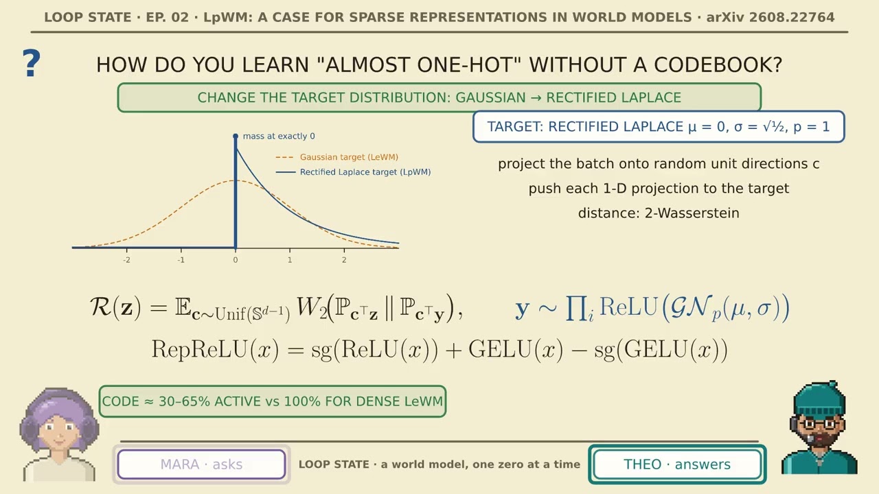
Achieving distributed sparsity in a JEPA without falling back on discrete codebooks, vector quantization (VQ), or brittle discrete bottlenecks requires reshaping the regularization objective. While LeWM matches features against a standard Gaussian, LpWM steers them toward a rectified generalized Gaussian—specifically, a zero-mean Laplace distribution passed through a ReLU activation.
Geometrically, a rectified Laplace distribution exhibits sharp exponential decay along the positive axis paired with a concentrated Dirac delta spike of probability mass sitting precisely at zero, representing all negative mass clipped by the rectification. The authors enforce this geometry using **RDMReg**, a regularizer that projects latent batches onto random unit directions and minimizes the 2-Wasserstein distance between empirical batch projections and the rectified target distribution.
To ensure coordinates reach exact zeros rather than merely vanishingly small values, the encoder's projector ends with a reparameterized ReLU: - **Forward pass:** Evaluates a strict standard ReLU, guaranteeing exact zeros. - **Backward pass:** Employs the gradient of a Gaussian Error Linear Unit (GELU) to prevent dead neurons and keep gradient flow healthy.
Depending on latent width, LpWM yields representations where 30% to 65% of coordinates are active, compared to 100% active density in LeWM. Crucially, reverting the target distribution back to a standard Gaussian without the rectification cleanly recovers LeWM. Because the encoder, predictor capacity, and CEM planner remain identical, this single distribution switch isolates sparsity as an independent variable.
[06:03](https://www.youtube.com/watch?v=FVpfCJfV110&t=363s) The Predictor Ladder and PushT Dynamics
To convert the theoretical claim of "simpler dynamics" into rigorous empirical metrics, the authors construct a ladder of predictors ranging from primitive linear models to deep transformers. By evaluating closed-loop planning success across this ladder, the specific rung where sparse latents succeed and dense latents fail serves as a direct gauge of dynamical simplicity.
```mermaid flowchart TD accTitle: Predictor Complexity Ladder accDescr: Hierarchy of predictor models evaluated in the paper, ranging from simple Linear Time-Invariant baselines to six-layer Diffusion Transformers. subgraph AttentionFree["Attention-Free Rungs (~3M to 85M Params)"] R1["LTI(1): Pure linear single-step (z_{t+1} = Az_t + Ba_t)"] R2["LTI(k): Linear with 3 frames of history"] R3["MLP ∘ LTI: Single ReLU layer over linear dynamics"] R4["MLP ∘ LTV: Linear Time-Varying (State-dependent matrices)"] end subgraph TransformerRungs["Transformer Predictors (Up to 822M Params)"] R5["1-Layer Transformer"] R6["6-Layer DiT (Standard LeWM predictor)"] end R1 --> R2 --> R3 --> R4 --> R5 --> R6 ```
The predictor ladder spans a massive scale: at a feature width of 4,096, the top-rung DiT contains 822 million parameters, while the bottom-rung LTI(1) uses only 34 million parameters, and the middle rungs hover between 70 and 85 million parameters. Architectures below the transformer level are entirely attention-free. Models are evaluated across five latent widths (from 384 to 4,096) utilizing Maximal Update Parameterization ($\mu\mathrm{P}$) to prevent hyperparameter drift across widths.
The experimental tests span two environments: 1. **Wall:** A simple 2D navigation task where an agent must locate a doorway. Because the underlying dynamics are trivial, even the bottom-rung LTI(1) predictor achieves nearly 100% closed-loop success across both sparse and dense representations, validating Wall as an intentionally designed null result. 2. **PushT:** A challenging benchmark requiring an agent to push a T-shaped block into a designated goal pose, involving complex contact mechanics, friction, and rotational discontinuities.
On PushT, both representations fail completely at the lowest LTI(1) rung, and both match high performance at the top transformer rungs. The entire distinction lives in the middle tiers: - **MLP $\circ$ LTI:** Sparse LpWM outperforms dense LeWM by **24 to 57 points** of planning success across widths. - **MLP $\circ$ LTV:** Sparse leads by **36 to 45 points**. - **LTI($k$):** Sparse leads by **11 to 23 points**.
Theo highlights a standout result from Figure 1B: at a width of 768 using the lightweight 3-million-parameter MLP $\circ$ LTI predictor, closed-loop planning achieves roughly **70% success on sparse codes** compared to a miserable **7% success on dense codes**. As Mara summarizes, the core value proposition is not necessarily building a marginally higher-scoring world model, but creating a radically cheaper, low-capacity world model that actually works.
[09:11](https://www.youtube.com/watch?v=FVpfCJfV110&t=551s) Ruling Out SIGReg and Validating Latent Support
Addressing potential skepticism, Mara questions whether the performance gap might simply reflect an idiosyncrasy or weakness of LeWM’s SIGReg regularizer rather than a fundamental flaw of dense codes. To test this, the authors evaluated a second dense baseline by substituting SIGReg with VICReg within the exact same setup.
When evaluated across the PushT ladder, sparse LpWM once again dominated across intermediate rungs like MLP $\circ$ LTV and MLP $\circ$ LTI. Intriguingly, against VICReg, LpWM even outperformed the dense baseline at the top-rung deep transformer. The authors hypothesize that because VICReg constrains only first- and second-order moments (variance and covariance), its target distribution remains underspecified, generating a geometrically degraded latent space for dynamics modeling; by contrast, SIGReg constrains the full distribution shape, making it a stronger dense competitor.
``` +------------------+---------------------+---------------------+ | Predictor Rung | Sparse LpWM vs LeWM | Sparse LpWM vs VICReg | +------------------+---------------------+---------------------+ | LTI(1) | Tie (Both fail) | Tie (Both fail) | | LTI(k) | Sparse +11 to +23 | Sparse wins | | MLP ∘ LTI | Sparse +24 to +57 | Sparse wins | | MLP ∘ LTV | Sparse +36 to +45 | Sparse wins | | Deep Transformer | Tie (Both succeed) | Sparse wins | +------------------+---------------------+---------------------+ ```
The discussion then turns to the mechanistic interpretation of the latent space: what are the inactive coordinates actually doing? To probe this, the authors engineered the **Piecewise** environment—an open room partitioned into hidden spatial zones, where each zone exerts a distinct constant directional force on the agent. The dynamics are locally linear within each region and globally piecewise-affine.
The authors evaluated the agent across a $20 \times 20$ spatial grid, binarizing each latent vector into its mathematical support (the binary mask of nonzero entries) and calculating the Jaccard similarity index (intersection over union) across spatial coordinates: - The binary support overlaps heavily among positions within the same dynamics zone and drops precipitously at regime boundaries. - Crucially, this zone-clustering behavior persists even when the visual markers of the zones are completely removed from the environment rendering, proving that the latent support latches onto the underlying physics rather than cosmetic visual textures. - Linear probe decoders reveal a striking separation of concerns, termed **mode factoring**: the binary support decodes the discrete physical zone with ~97% accuracy (matching the full continuous vector), while continuous coordinate positions within a zone are decoded primarily from coordinate magnitudes. - In planning evaluations over random goals within Piecewise, sparse models attained **84.7% success** compared to **65.3% for dense models**, maintaining their performance edge across extended planning horizons.
Turning finally to contact-rich robotic manipulation in the OGBench-Cube environment—where discrete dynamical transitions represent physical contact between the gripper and the cube—the hosts note the paper's transparency regarding the limits of vanilla sparsity and support stability.
[12:27](https://www.youtube.com/watch?v=FVpfCJfV110&t=747s) Does It Still Work When Things Touch? Support Dynamics on OGBench-Cube
When testing whether the sparsity pattern naturally tracks physical contact on the OGBench-Cube manipulation task, the initial results show an immediate limitation of pure marginal regularization. Out of the box, the latent support shifts whenever the robotic arm moves across the workspace. The support correlates at 0.87 with end-effector motion, while its correlation with actual object contact hovers at an insignificant 0.05. As the hosts observe, without additional inductive biases, "the zeros are just a motion detector." Because RDMReg exclusively penalizes and shapes the marginal feature distribution frame by frame, it possesses no temporal awareness across transitions.
```mermaid flowchart TD accTitle: Temporal Jaccard Loss Effect on Latent Support accDescr: Diagram illustrating how adding temporal Jaccard loss redirects the latent zero support from tracking arm motion to tracking physical contact and cube motion. subgraph Raw["Vanilla RDMReg (Marginal Only)"] direction TB A1["Frame-level Laplace Prior"] --> B1["Latent Support Pattern"] B1 --> C1["End-Effector Motion (r = 0.87)"] B1 -.->|Weak signal| D1["Object Contact (r = 0.05)"] end subgraph Regularized["RDMReg + Temporal Jaccard Prior"] direction TB A2["Temporal Jaccard Loss"] --> B2["Penalize Inter-Frame Support Flips"] B2 --> C2["Latent Support Stabilizes"] C2 --> D2["Cube Motion (r = 0.80)"] C2 --> E2["Physical Contact (r = 0.61)"] end ```
To bridge this gap, the authors introduce an optional temporal Jaccard loss that explicitly penalizes support flips between adjacent time steps. Adding this temporal prior completely realigns what the zero patterns encode without degrading planning performance:
- Correlation with end-effector motion plummets from 0.87 down to 0.40. - Correlation with cube motion climbs significantly up to 0.80. - Correlation with physical contact jumps from 0.05 to 0.61. - Planning success rate remains stable throughout tuning, proving that reallocating support semantics does not harm task execution. - Raster plots reveal that the active support becomes quiet during free space navigation and sharply reorganizes when entering the contact interaction window. - The fundamental mechanism is summarized neatly: "Sparsity gives you a slot for the mode. A temporal prior decides what goes in the slot."
---
[13:34](https://www.youtube.com/watch?v=FVpfCJfV110&t=814s) What Does This Paper Not Show? Theoretical and Empirical Limitations
Turning to the boundaries of the paper, the hosts scrutinize the exact failure modes, omissions, and assumptions underpinning LpWM. The most significant empirical asterisk is that sparse representations do not beat dense representations when paired with high-capacity predictors: on PushT, when using a Diffusion Transformer (DiT) backbone, sparse and dense representations achieve parity. The massive performance deltas only materialize at intermediate predictor capacity.
The gap between the mathematical theory and practical implementation is equally sharp. The paper's formal linearization proof (Proposition 1) relies on strictly one-hot latent codes, which demand exponentially many dimensions relative to state space complexity. In contrast, the trained networks produce codes with 30% to 65% active coordinates, operating far from true one-hot regimes. The mathematical proof serves as an inspirational motivation for local linearity rather than an exact description of the empirical model.
The experimental design also leaves several practical questions open:
- **Benchmark Diversity:** Evaluated across four environments, all of which are simulated; three are purely two-dimensional navigation or planar pushing benchmarks, with zero physical robot validation. - **Statistical Rigor:** Models were trained across only a single training seed and evaluated on three test seeds, reporting numbers from the best-performing tuned hyperparameter cells. - **Interpretability Prerequisite:** Support interpretation is completely unsupervised only when physical modes are purely spatial (as in the Piecewise domain); on contact benchmarks like Cube, it requires a hand-tuned, optional auxiliary temporal loss. - **Missing Categorical Baselines:** The study does not include direct head-to-head empirical comparisons against discrete latent frameworks like DreamerV2's categorical distributions, despite referencing them in related work. - **Author Aspirations vs. Present Evidence:** The paper positions latent Linear Quadratic Regulator (LQR) control and the hypothesis that sparsity benefits will scale up to heavy transformer backbones under harder dynamics strictly as future work rather than demonstrated results.
---
[15:06](https://www.youtube.com/watch?v=FVpfCJfV110&t=906s) Key Takeaways and Open Questions
In their closing reflections, the hosts highlight the broader paradigm shift implied by the paper. The geometry of a world model's latent space should not default to an isotropic Gaussian blob simply because self-supervised learning conventions inherited from computer vision dictate it. Latent geometry is an explicit system design choice. Introducing true zeros into the representation simplifies the learning burden on the physics engine, providing discrete structural slots that signal which physical regime the system occupies.
The episode leaves listeners with a core open challenge for model-based reinforcement learning: at what threshold of dynamical complexity does even a heavy transformer like a DiT begin to fail on dense geometries and actively demand sparse representations? While the current experiments stop just short of proving that transition point, the paper lays the architectural foundation for testing it.
## Notable quotes > [00:00](https://www.youtube.com/watch?v=FVpfCJfV110&t=0s) Why does every world model squeeze its features into a Gaussian blob?
> [02:51](https://www.youtube.com/watch?v=FVpfCJfV110&t=171s) What if the code were one-hot?
> [02:51](https://www.youtube.com/watch?v=FVpfCJfV110&t=171s) a lookup table wearing a linear algebra costume. — Mara
> [04:30](https://www.youtube.com/watch?v=FVpfCJfV110&t=270s) How do you learn "almost one-hot" without a codebook?
> [06:03](https://www.youtube.com/watch?v=FVpfCJfV110&t=363s) How do you measure "simpler dynamics"?
> [09:11](https://www.youtube.com/watch?v=FVpfCJfV110&t=551s) Is this just SIGReg being weak? — Mara
> [09:11](https://www.youtube.com/watch?v=FVpfCJfV110&t=551s) What do the zeros mean?
> [12:27](https://www.youtube.com/watch?v=FVpfCJfV110&t=747s) Does it still work when things touch?
> [12:27](https://www.youtube.com/watch?v=FVpfCJfV110&t=747s) the zeros are just a motion detector.
> [12:27](https://www.youtube.com/watch?v=FVpfCJfV110&t=747s) Sparsity gives you a slot for the mode. A temporal prior decides what goes in the slot.
> [13:34](https://www.youtube.com/watch?v=FVpfCJfV110&t=814s) What does this paper not show?
## Mentioned Yann LeCun, Mara, Theo, Loop State, LpWM, LeWM, VICReg, SIGReg, RDMReg, JEPA, PushT, OGBench-Cube, DreamerV2, Lean 4, Claude Fable 5.1
## Video description Should a world model's latent code be dense or sparse? Every JEPA world model pushes its features toward a Gaussian blob. This paper from Yann LeCun's group (Kuang, Dagade, Le Lidec, Maes, Balestriero, LeCun, August 2026) asks whether that is the wrong shape, and shows that codes with exact zeros make the dynamics simpler to learn: a 3M-parameter predictor plans at ~70% on sparse codes where it gets ~7% on dense ones.
Loop State EP. 02. Two hosts, Mara and Theo, walk the paper one question at a time.
Chapters 0:00 Why does every world model squeeze its features into a Gaussian blob? 1:20 What is a JEPA world model actually predicting? 2:51 What if the code were one-hot? 4:30 How do you learn "almost one-hot" without a codebook? 6:03 How do you measure "simpler dynamics"? 7:37 Where does sparsity actually win? 9:11 Is this just SIGReg being weak? 10:22 What do the zeros mean? 12:14 Does it still work when things touch? 13:41 What does this paper not show? 15:12 Sign-off
What the paper shows - RDMReg swaps LeWM's Gaussian target for a Rectified Laplace, so 30–65% of latent coordinates are exactly zero. Everything else (encoder, predictor, CEM planner) is shared. - Proposition 1: one-hot codes turn any Lipschitz controlled dynamics into exactly linear latent dynamics, at the price of exponentially many dimensions. - On PushT, sparse beats dense by 24–57 points (MLP∘LTI), 36–45 (MLP∘LTV), 11–23 (LTI(k)) at intermediate predictor capacity. Ties at the DiT rungs. Both fail at LTI(1). - The sparse advantage survives a second dense baseline (VICReg). - The zeros are interpretable: on Piecewise, the binary support decodes the dynamics zone (0.97) even with no visual cues, and magnitudes decode position. On OGBench-Cube, the support only tracks contact once a temporal-Jaccard prior is added.
What it does not show No win over dense codes with a strong predictor, four simulated environments and no real robot, one training seed with three evaluation seeds, and no head-to-head with discrete latents like DreamerV2's categoricals.
Paper: https://arxiv.org/abs/2608.22764 Figures are rasterized from the arXiv e-print. Concept diagrams and pixel-art hosts were authored for this episode. Voices: MiniMax speech-2.8-hd. Board rendered with Leanim (Lean 4). Produced with Claude Fable 5.1.
#WorldModels #JEPA #SparseRepresentations #SelfSupervisedLearning #Robotics #MachineLearning #YannLeCun #AIResearch
The chapter timestamps are computed from the frozen narration manifest. Verify them against the upload once, since YouTube requires the first stamp to be 0:00 and at least three stamps to show chapter markers, both of which this list satisfies.
[Source](https://www.youtube.com/watch?v=FVpfCJfV110)