RWKV Speeds Batched Inference 7.2-Fold With Frozen 3B Backbone

Xiaol.x

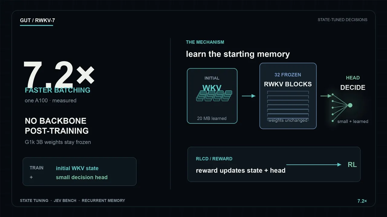
Adapting a 20-megabyte initial recurrent memory state delivers a 7.2-fold execution speedup without backbone retraining, though the compressed representation collapses on boolean and multi-step reasoning.

AI-assisted summary of Gut Feeling: RWKV + JEV — 7.2× Faster Decisions with State Tuning — original source. Check the original for full context.

Source published: 2026-09-25

Key ideas

By tuning only a learned initial WKV state (~20 MiB) and a lightweight decision head, a frozen G1k 3B RWKV backbone achieved a 7.2× within-request batching speedup on an A100 GPU. (0:00)
In a separate public evaluation, the adapted recurrent model attained 64.5% accuracy (149/231 tasks) with 100% schema validity, though performance degraded sharply on complex reasoning queries. (0:00)
At an 8k context length, the constant 20.31 MiB recurrent state offers a 14.18× memory reduction compared to a standard 3B Transformer's expanding KV cache. (6:29)
Despite pristine schema formatting, severe blind spots emerged, including a near-total failure mode on boolean queries where the model defaulted to 'false' on 471 out of 472 inputs. (4:24)

Detailed notes

## Background Published on YouTube by Xiaol.x on September 25, 2026, this video examines how a pretrained 3B recurrent RWKV model can adapt to structured decision tasks without updating its core weights. According to the description, it demonstrates a 7.2× within-request batching speedup on an A100 GPU by training only an initial WKV state and a small decision head, alongside an empirical evaluation on public JevBench tasks.

## TL;DR The video demonstrates state tuning on a frozen G1k 3B RWKV backbone, adapting the model to structured decision tasks by optimizing only roughly 20 MiB of initial recurrent memory and a compact classification head via RLCD and policy gradients. Across 32 repeated queries on an A100 GPU, within-request batching achieved a 7.2× speedup compared to serial execution, while maintaining a fixed 20.3125 MiB live state per stream that avoids Transformer KV cache bloat. In a separate evaluation on 231 public tasks, the model scored 64.5% accuracy with 100% schema validity, though it exhibited severe blind spots such as near-total collapse on boolean questions and weak performance on multi-hop reasoning.

## Atmosphere & style The presentation carries a meticulous, engineering-first tone characterized by intellectual honesty and measured restraint. Rather than leaning into hyperbole around artificial intelligence breakthroughs, the presenter candidly dissects system limitations, walking viewers step-by-step through tensor math, memory matrices, and catastrophic edge-case failures like the near-uniform false predictions on boolean queries. It feels like an open-source technical post-mortem and lab walkthrough, pairing precise code mechanics with clear caveats distinguishing micro-benchmarks from production server concurrency.

## Bulletin - [00:00](https://www.youtube.com/watch?v=hRsQZ8Qb8vA&t=0s) By tuning only a learned initial WKV state (~20 MiB) and a lightweight decision head, a frozen G1k 3B RWKV backbone achieved a 7.2× within-request batching speedup on an A100 GPU. - [00:00](https://www.youtube.com/watch?v=hRsQZ8Qb8vA&t=0s) In a separate public evaluation, the adapted recurrent model attained 64.5% accuracy (149/231 tasks) with 100% schema validity, though performance degraded sharply on complex reasoning queries. - [06:29](https://www.youtube.com/watch?v=hRsQZ8Qb8vA&t=389s) At an 8k context length, the constant 20.31 MiB recurrent state offers a 14.18× memory reduction compared to a standard 3B Transformer's expanding KV cache. - [04:24](https://www.youtube.com/watch?v=hRsQZ8Qb8vA&t=264s) Despite pristine schema formatting, severe blind spots emerged, including a near-total failure mode on boolean queries where the model defaulted to 'false' on 471 out of 472 inputs.

## Key takeaways - [00:00](https://www.youtube.com/watch?v=hRsQZ8Qb8vA&t=0s) The G1k 3B backbone remains completely frozen during adaptation, with updates restricted to ~20 MiB of initial recurrent memory state and a compact decision head. - [00:00](https://www.youtube.com/watch?v=hRsQZ8Qb8vA&t=0s) The reported 7.2× speedup measures within-request batched execution (1.018 s vs. 7.330 s serial) for 32 repeated questions on an A100 GPU, rather than concurrent multi-client server throughput. - [00:00](https://www.youtube.com/watch?v=hRsQZ8Qb8vA&t=0s) On public JevBench tasks, state tuning yielded 149 of 231 correct answers (64.5%) with zero schema violations, serving as a standalone evaluation rather than an official leaderboard rank. - [00:56](https://www.youtube.com/watch?v=hRsQZ8Qb8vA&t=56s) The RWKV recurrent state spans 32 layers with 40 heads per layer, where each head maintains a 64×64 associative matrix memory alongside auxiliary token-shift history vectors. - [02:05](https://www.youtube.com/watch?v=hRsQZ8Qb8vA&t=125s) Adaptation is achieved via RLCD and policy gradient updates applied directly to the learned starting state before prompt context enters the recurrent loop. - [02:05](https://www.youtube.com/watch?v=hRsQZ8Qb8vA&t=125s) Policy gradient training optimizes 16 positive and negative perturbation pairs while reusing a single forward evaluation of the backbone per question. - [03:32](https://www.youtube.com/watch?v=hRsQZ8Qb8vA&t=212s) Task accuracy proved highly sensitive to optimization hyperparameters; simply lowering the state learning rate raised task cohort accuracy from 38/72 to 56/72. - [04:24](https://www.youtube.com/watch?v=hRsQZ8Qb8vA&t=264s) The adapter struggles with structured reasoning, recording 16.7% accuracy on trade-off questions, 20.0% on probability queries, and 27.8% on multi-hop composition. - [04:24](https://www.youtube.com/watch?v=hRsQZ8Qb8vA&t=264s) A full regression occurred on boolean questions, with the system predicting 'false' on 471 of 472 inputs, demonstrating that schema compliance does not ensure logical calibration. - [05:15](https://www.youtube.com/watch?v=hRsQZ8Qb8vA&t=315s) The recurrent state requires exactly 20.0 MiB in FP32 for head matrices plus 0.3125 MiB in FP16 for token history vectors, creating a constant 20.3125 MiB runtime footprint per stream. - [06:29](https://www.youtube.com/watch?v=hRsQZ8Qb8vA&t=389s) In a 24 GiB VRAM budget at 8k context tokens, RWKV's fixed state allows theoretical room for 1,209 resident stream slots compared to 85 slots for a standard 3B Transformer. - [06:29](https://www.youtube.com/watch?v=hRsQZ8Qb8vA&t=389s) Theoretical slot occupancy does not directly translate to multi-tenant concurrency due to prompt prefill overheads, candidate evaluation demands, and server scheduling bottlenecks. - [08:04](https://www.youtube.com/watch?v=hRsQZ8Qb8vA&t=484s) State-tuned recurrent models provide a viable path toward low-latency, bounded decision APIs without post-training full multi-billion parameter backbones.

## Detailed walkthrough ### [00:00](https://www.youtube.com/watch?v=hRsQZ8Qb8vA&t=0s) Results Overview and Frozen Backbone Adaptation

The core takeaway is delivered upfront: a 7.2× speedup achieved through within-request batching on an A100 GPU without any post-training of the G1k 3B recurrent backbone. The underlying model weights remain completely frozen; the only components updated during adaptation are the learned starting memory state and a lightweight decision head. In parallel, a separate supervised state-tuning evaluation on public JevBench tasks yields an accuracy of 64.5% (149 out of 231 tasks correct), with 100% of the model outputs maintaining schema validity. The presenter is careful to qualify these figures immediately: this is a standalone public evaluation rather than an official JevBench leaderboard submission, and the batching speedup measures within-request optimization rather than concurrent multi-client server throughput.

To demonstrate how the system works in practice, the video introduces a concrete customer service routing task: `"I was charged twice. Please refund the extra payment."` In an earlier 0.4B pilot experiment, this ticket was correctly categorized and routed to billing. The goal is to understand how this tokenized message flows through the recurrent memory structure and yields a structured decision without modifying the billions of weights inside the backbone.

- **Speedup:** 7.2× faster execution using batched evaluation on a warm A100 40GB GPU. - **Backbone State:** Pretrained G1k 3B backbone weights remain entirely frozen. - **Trainable Footprint:** ~20 MiB of initial recurrent memory state plus a compact decision head. - **Quality Metric:** 149/231 (64.5%) on public JevBench tasks, with every response schema-valid.

---

[00:56](https://www.youtube.com/watch?v=hRsQZ8Qb8vA&t=56s) Deconstructing the Recurrent RWKV State

Peeling back the layers of a single RWKV block reveals how tokens interact with the recurrent architecture. As an incoming token enters a block, it first encounters TimeMix, which inspects and updates a persistent matrix memory before passing its output through a residual connection back into the token vector. From there, ChannelMix applies a feed-forward channel transformation, accompanied by a second residual addition. This sequence cascades across all 32 layers of the network.

```mermaid flowchart TD accTitle: RWKV Block State Flow accDescr: Diagram showing TimeMix and ChannelMix updates with residual connections and state memory in an RWKV block.

subgraph Block["RWKV Block (1 of 32)"] direction TB TokenIn["Token Vector In"] TM["TimeMix"] CM["ChannelMix"] TokenOut["Token Vector Out"]

TokenIn --> TM TokenIn -->|"Residual 1"| TM TM --> CM TM -->|"Residual 2"| CM CM --> TokenOut end

subgraph StateMem["Recurrent State Memory"] direction TB WKV["40 Heads x (64x64) Matrix"] Hist["Token History Vectors (TM & CM)"] end

The concept of "states inside a state" becomes tangible when inspecting the dimensional hierarchy: - **Depth:** 32 sequential layers. - **Attention/Mixing Heads:** 40 heads per layer. - **Head State:** Each individual head maintains a 64×64 state matrix. - **Token History Vectors:** Two smaller auxiliary vectors per layer capture the immediately preceding inputs to TimeMix and ChannelMix to facilitate token-to-token shift comparisons, distinct from the primary associative matrix memory.

Within each head matrix, past associations are retained, decayed over time, corrected, and overwritten with fresh associations as new tokens arrive. The video emphasizes that conceptual diagrams reflect the mathematical and structural mechanics of the code rather than empirical activation maps: the design provides an intuition for a compact situational representation, not a "verified world simulator."

---

[02:05](https://www.youtube.com/watch?v=hRsQZ8Qb8vA&t=125s) State Tuning via RLCD and Policy Gradients

Rather than fine-tuning the 3-billion-parameter backbone, training is confined strictly to the initial WKV memory state and the decision head. This learned starting state enters the recurrent loop before any prompt context arrives; it acts as a learned prior rather than an additional adapter layer tacked onto the end of the model.

```mermaid flowchart LR accTitle: Training vs Inference Recurrent State Flow accDescr: Diagram contrasting policy and RLCD updates during training with static initial memory during inference.

subgraph Train["Training Phase (Backbone Frozen)"] direction TB InitStateTrain["Learned Initial WKV State"] PromptTrain["Prompt Tokens"] BBTrain["Frozen G1k 3B Backbone"] HeadTrain["Decision Head"] RewardGrad["Reward / Policy Updates\n(Pathwise or REINFORCE)"]

InitStateTrain --> BBTrain PromptTrain --> BBTrain BBTrain --> HeadTrain HeadTrain --> RewardGrad RewardGrad -.->|"Update State & Head"| InitStateTrain RewardGrad -.->|"Update State & Head"| HeadTrain end

subgraph Infer["Inference Phase"] direction TB InitStateInfer["Fixed Learned State"] BBInfer["Frozen G1k 3B Backbone"] Output["Typed Decision Output"]

InitStateInfer --> BBInfer BBInfer --> Output end ```

The optimization framework leverages Reinforcement Learning from Compiler/Diagnostic Feedback (RLCD) and policy gradient formulations: - **Legacy RLCD:** Adds perturbation noise directly to output logits and differentiates through a scoring reward function. - **Revised Policy Experiment:** Evaluates 32 noisy logit vectors derived from 16 positive and negative perturbation pairs. Crucially, these pairs reuse a single forward evaluation of the backbone per question rather than executing 32 separate autoregressive rollouts. - **Reward Signals:** Ground-truth target labels inform the reward, log-probabilities, and a spherical score metric, combined with an ordinal distance penalty applied specifically to score evaluations. - **Update Paths:** Both pathwise reward gradients (which differentiate directly through the scoring mechanism) and REINFORCE-style updates (which scale gradients by reward-weighted log probabilities) route parameter updates exclusively to the initial state and the decision head.

Once training concludes, exploratory noise, sampling perturbations, and optimizer updates are stripped away. During inference, while the live recurrent state continues to evolve dynamically with every ingested token, the learned starting state remains static.

---

[03:32](https://www.youtube.com/watch?v=hRsQZ8Qb8vA&t=212s) Benchmark Accuracy and Failure Modes

On out-of-domain evaluation tasks where the adapter must produce structured, typed answers, performance proved highly sensitive to hyperparameter tuning: - **Early Public Baseline:** Initially achieved 38 out of 72 correct answers. - **Learning Rate Sensitivity:** Simply reducing the state learning rate boosted accuracy on the matched cohort to 56 of 72, edging out the pathwise reward branch by one task. - **Full Public Cohort:** On the broader 231-task public distribution, the lower learning rate cross-entropy run answered 149 of 231 tasks (64.5%), with 100% schema compliance. On a local A100 GPU, median serial request execution took approximately one-third of a second.

Despite strong schema validity, the model exhibits sharp blind spots, proving that a cleanly typed answer can still be "confidently wrong":

The near-complete failure on boolean queries—defaulting to `false` in all but one instance—highlights that the compressed state fails to carry complex multi-step reasoning dependencies, underscoring the absolute necessity of rigorous held-out calibration checks before deploying decisions into production.

---

[05:15](https://www.youtube.com/watch?v=hRsQZ8Qb8vA&t=315s) Memory Footprint and Recurrent State Math

The exact parameter and memory math of the recurrent state illustrates why recurrent architectures provide an operational advantage for structured inference:

$$\text{Matrix Parameters} = 32 \text{ layers} \times 40 \text{ heads} \times (64 \times 64) = 5{,}242{,}880 \text{ elements}$$

Stored in 4-byte single-precision floating point (FP32), these matrix elements equate to exactly:

$$5{,}242{,}880 \times 4 \text{ bytes} = 20{,}971{,}520 \text{ bytes} = 20\text{ MiB}$$

The auxiliary input history vectors for TimeMix and ChannelMix store 2-byte values (FP16/BF16), contributing an additional 0.3125 MiB across the 32 layers. Consequently, a single active recurrent stream occupies exactly 20.3125 MiB, matching the repository's empirical memory allocation.

``` Total Live State Memory per Branch: • Head State Matrices (FP32): 20.0000 MiB • Token History Vectors (FP16): 0.3125 MiB ------------------------------------------- Total Recurrent State: 20.3125 MiB

Static Adapter Overhead: • Trainable Decision Head: ~1.2700 MiB ------------------------------------------- Total Adapter Tensors: ~21.2700 MiB ```

While the learned initial state is shared across requests, each concurrent branch or active user must maintain its own private 20.3125 MiB state. For example, a batch of 16 independent decision streams demands roughly 325 MiB of dedicated GPU memory for states alone, beyond backbone weights and workspace buffers.

---

[06:29](https://www.youtube.com/watch?v=hRsQZ8Qb8vA&t=389s) Capacity Estimation vs. Transformers and Batched Speed

To evaluate memory capacity, the presenter contrasts RWKV against a standard Grouped-Query Attention (GQA) Transformer: Qwen 2.5 3B (36 layers, 2 key-value heads, head dimension of 128).

At 2 bytes per entry, the Transformer's KV cache expands continuously at 36 KiB per token:

$$\text{KV Cache at 8,192 tokens} = 8{,}192 \times 36\text{ KiB} = 294{,}912\text{ KiB} = 288\text{ MiB}$$

Comparing 288 MiB per stream to RWKV's constant 20.3125 MiB yields a memory footprint ratio of **14.18×** in favor of RWKV at long context lengths.

``` Resident Stream Slots in 24 GiB Free VRAM (at 8k Context): • Standard Transformer (Qwen 2.5 3B, 16-bit KV): 85 streams • Gated RWKV G1k 3B State: 1,209 streams ```

Quantizing the Transformer KV cache to 8-bit cuts that memory advantage roughly in half. Crucially, the presenter notes that theoretical slot occupancy does not equate to realized multi-tenant concurrency. Actual throughput depends heavily on prompt prefill speeds, candidate evaluation costs, custom CUDA kernels, and batch scheduling.

The empirical speedup measured in the repository—**7.2× faster execution** (reducing 7.330 seconds of serial execution to 1.018 seconds batched)—evaluates 32 repeated questions packed into a single shared-prefix request on an A100. Because the current test server serializes incoming clients, formal claims regarding multi-client server throughput and tail latency remain subject to future testing.

---

[08:04](https://www.youtube.com/watch?v=hRsQZ8Qb8vA&t=484s) Bounded Decision APIs and Future Benchmarks

The overarching architecture distills into a clean pipeline: an incoming support ticket passes into the frozen G1k 3B backbone initialized with the learned recurrent state, terminating in branched output heads configured for structured choices, boolean outcomes, or continuous score predictions.

This creates a bounded, low-latency decision API that exploits recurrent state reuse without ballooning memory. However, critical research questions persist around improving data splits, modeling cross-candidate interactions, and remedying probability miscalibration on multi-hop questions. Gated RWKV illustrates a highly viable path toward turning a 3B recurrent model into a specialized Jev-style decision engine, but it does not claim to be an off-the-shelf general reasoner. The core breakthrough remains effective task adaptation achieved solely by tuning a 20 MiB starting memory and a tiny head, leaving the 3-billion-parameter backbone entirely untouched.

## Notable quotes > [00:00](https://www.youtube.com/watch?v=hRsQZ8Qb8vA&t=0s) What if a 3B recurrent model could adapt to a structured decision task without updating its backbone?

> [00:00](https://www.youtube.com/watch?v=hRsQZ8Qb8vA&t=0s) 7.2× faster within-request batching on one A100, while the pretrained G1k 3B backbone stays frozen.

> [00:00](https://www.youtube.com/watch?v=hRsQZ8Qb8vA&t=0s) 149/231 = 64.5%, with every response schema-valid.

> [00:00](https://www.youtube.com/watch?v=hRsQZ8Qb8vA&t=0s) this is not an official JevBench leaderboard rank and it is not a concurrent-client throughput claim.

> [00:00](https://www.youtube.com/watch?v=hRsQZ8Qb8vA&t=0s) I was charged twice. Please refund the extra payment.

> [00:56](https://www.youtube.com/watch?v=hRsQZ8Qb8vA&t=56s) states inside a state

> [03:24](https://www.youtube.com/watch?v=hRsQZ8Qb8vA&t=204s) confidently wrong

> [03:24](https://www.youtube.com/watch?v=hRsQZ8Qb8vA&t=204s) predicts false on 471 / 472 inputs

## Mentioned RWKV, G1k 3B, JEV, JevBench, A100, A100 40GB, TimeMix, ChannelMix, RLCD, REINFORCE, Qwen 2.5 3B, GitHub

## Video description What if a 3B recurrent model could adapt to a structured decision task without updating its backbone?

In this video, we open with the measured result: **7.2× faster within-request batching** on one A100, while the pretrained G1k 3B backbone stays frozen. The trainable pieces are the learned initial WKV state and a small decision head. We then unpack the actual RWKV state, show how RLCD and reward-based state tuning update that memory, and follow one real decision from a customer message to a typed output.

The video also reports a separate public-task evaluation: **149/231 = 64.5%**, with every response schema-valid. That quality number and the batching number come from separate experiments; this is not an official JevBench leaderboard rank and it is not a concurrent-client throughput claim.

We visualize:

- the initial WKV state → 32 frozen RWKV blocks → decision head; - TimeMix, ChannelMix, residual paths, and the recurrent update; - nested state structure: 32 layers × 40 heads × 64×64 WKV matrices; - RLCD and REINFORCE-style reward updates to the state and head; - state memory, resident slots, and the measured batching path.

Project and research notes: https://github.com/xiaol/Gut-RWKV-Jev-laya

Chapters

00:00 The result first 00:56 Open the recurrent state 02:05 RL tunes the starting memory 03:32 Watch the decision happen 04:24 Where the story breaks 05:15 Twenty megabytes of learned starting memory 06:29 Estimate capacity, measure speed 08:04 What the result really says

Evidence notes

- The 7.2× result compares 7.330 s serial execution with 1.018 s batched execution for 32 repeated three-option questions, using a warm A100 40GB run and a shared prefix. - The 64.5% result is a separate cross-entropy state/head evaluation on 149 of 231 public tasks. - Backbone weights remain frozen. State/head adaptation is still training, but it does not post-train the G1k 3B backbone. - No claim is made that this is a top-ranked JevBench submission or that it measures multi-client server concurrency.

#RWKV #JevBench #StateTuning #ReinforcementLearning #RecurrentNeuralNetwork #MachineLearning

[Source](https://www.youtube.com/watch?v=hRsQZ8Qb8vA)

中文简报

RWKV利用冻结的3B主干网络将批处理推理速度提升7.2倍通过微调20MB的初始循环记忆状态，在无需重新训练主干网络的情况下实现了7.2倍的执行加速，但该压缩表征在布尔与多步推理上出现崩溃。该视频展示了在冻结的G1k 3B RWKV主干网络上进行状态微调，通过RLCD和策略梯度仅优化约20 MiB的初始循环记忆以及一个紧凑的分类头，使模型适应结构化决策任务。在A100 GPU上针对32个重复查询的测试中，请求内批处理相比串行执行实现了7.2倍的加速，同时每个数据流保持固定的20.3125 MiB实时状态，避免了Transformer KV缓存膨胀的问题。在针对231个公开任务的另一项评估中，该模型取得了64.5%的准确率和100%的模式有效性，但同时也暴露出严重的盲区，例如在布尔问题上近乎完全崩溃，且在多跳推理上表现较弱。通过仅微调学习到的初始WKV状态（约20 MiB）和一个轻量级决策头，冻结的G1k 3B RWKV主干网络在A100 GPU上实现了7.2倍的请求内批处理加速。 (0:00) 在另一项公开评估中，调优后的循环模型达到了64.5%的准确率（149/231个任务）和100%的模式有效性，但在复杂推理查询上性能急剧下降。 (0:00) 在8k上下文长度下，固定为20.31 MiB的循环状态相比标准3B Transformer不断膨胀的KV缓存，内存占用减少了14.18倍。 (6:29) 尽管模式格式完全合规，但模型暴露出了严重的盲区，包括在布尔查询上近乎完全失效，在472个输入中有471个默认输出为“false”。 (4:24)

Reading summary

Xiaol.x demonstrates that state tuning on a frozen 3-billion-parameter RWKV backbone—updating only a learned ~20 MiB initial recurrent memory state and a compact decision head—enables structured decision routing while achieving a 7.2× within-request batched speedup on an A100 GPU. Frozen Backbone Adaptation and Recurrent State Math (0:00) Rather than fine-tuning the 3-billion-parameter G1k backbone, the adaptation architecture keeps all underlying model weights completely frozen. Training is restricted to a learned starting recurrent memory state and a lightweight ~1.27 MiB decision head. Inside each of the network's 32 layers, token representations pass through TimeMix and ChannelMix operations across 40 heads. Each head maintains a 64×64 state matrix, totaling 5,242,880 elements. Stored in 4-byte FP32 precision, these matrices require exactly 20.0 MiB of memory, with auxiliary 2-byte token history vectors adding 0.3125 MiB across the layers for a total active recurrent footprint of 20.3125 MiB per stream. This learned initial state operates as a prior that enters the recurrent loop before any prompt tokens arrive, functioning as a contextual bias rather than an adapter tacked onto the model's output. While the learned initial state is shared across calls, each independent concurrent decision stream must maintain its own private 20.3125 MiB state buffer during evaluation, requiring roughly 325 MiB of GPU memory for a batch of 16 streams beyond the frozen model weights. Optimization via Perturbed Policy Updates and RLCD (2:05) The training methodology adapts the initial recurrent state and decision head using Reinforcement Learning from Compiler/Diagnostic Feedback (RLCD) and policy gradient formulations. In the revised policy setup, the system evaluates 32 perturbed logit vectors derived from 16 positive and negative perturbation pairs. Crucially, these paired evaluations share a single forward pass through the frozen backbone per question, avoiding the compute overhead of 32 separate autoregressive rollouts. Parameter updates route through both pathwise reward gradients—which differentiate directly through scoring functions informed by ground-truth labels, spherical metrics, and ordinal distance penalties—and REINFORCE-style policy gradients. Once training concludes, all perturbation noise, sampling logic, and optimizer updates are stripped away. During inference, the learned starting state remains fixed, while the live recurrent memory updates dynamically with each incoming token. Benchmark Accuracy, Schema Adherence, and Reasoning Limitations (3:32) On public JevBench evaluation tasks, performance proved highly sensitive to hyperparameter tuning. While an initial baseline achieved 38 out of 72 tasks correct, lowering the state learning rate raised accuracy on that cohort to 56 of 72. Evaluated on the broader 231-task public distribution, the lower learning rate cross-entropy run answered 149 tasks correctly (64.5%) with 100% schema validity and an ordinal mean absolute error of 0.134, recording a median serial execution time of about one-third of a second on an A100 GPU. Despite perfect schema compliance, the model exhibited severe reasoning blind spots. Accuracy fell to 16.7% on trade-off questions, 20.0% on probability queries, and 27.8% on multi-hop composition tasks. Most notably, the model experienced a near-total collapse on boolean questions, predicting false in 471 out of 472 instances. Paired with an expected calibration error of 0.21, these results demonstrate that while the recurrent state produces cleanly formatted outputs, it fails on complex relational dependencies without strict calibration. Memory Scaling Against Transformers and Batched Speedup (6:29) Comparing RWKV against a standard Grouped-Query Attention Transformer, such as Qwen 2.5 3B, illustrates the structural difference in memory scaling. A Transformer's 16-bit key-value cache expands continuously at 36 KiB per token, reaching 288 MiB per stream at an 8,192-token context length. RWKV's fixed 20.3125 MiB state yields a 14.18× memory advantage at that sequence length, theoretically allowing 1,209 resident streams in 24 GiB of free VRAM compared to 85 for the Transformer. In execution benchmarks on an A100 GPU, packing 32 repeated prompts into a single shared-prefix request dropped runtime from 7.330 seconds to 1.018 seconds, realizing a 7.2× speedup. However, the presenter qualifies that this test isolates within-request batching rather than multi-client server concurrency, as the evaluation server serialized incoming client requests and did not measure multi-tenant throughput or tail latency. The presented architecture shows that tuning a 20 MiB starting memory and a small output head can adapt a frozen 3B recurrent model into a fast, schema-compliant decision API. However, unresolved challenges remain around severe probability miscalibration on multi-hop problems, boolean regression, and measuring true multi-client server throughput beyond shared-prefix batching.

Source quotes

[0:00] What if a 3B recurrent model could adapt to a structured decision task without updating its backbone? [0:00] 7.2× faster within-request batching on one A100, while the pretrained G1k 3B backbone stays frozen. [0:00] 149/231 = 64.5%, with every response schema-valid. [0:00] this is not an official JevBench leaderboard rank and it is not a concurrent-client throughput claim. [0:00] I was charged twice. Please refund the extra payment. [0:56] states inside a state [3:24] confidently wrong [3:24] predicts false on 471 / 472 inputs

Original transcript

[0:00] 7.2 times faster through batching with [0:03] no post training of the G1K3B [0:06] backbone. [0:08] Its weights stay frozen. [0:10] Only the starting state and a small head [0:12] are trained. [0:14] >> Separately, on the public GEB bench [0:16] tasks, supervised state tuning scores [0:18] 64.5%. [0:20] Every response is schema valid. That is [0:23] a public evaluation, not an official [0:25] leaderboard rank. [0:27] >> The G1K3B backbone stays frozen. We [0:31] train 20 mebibytes of starting memory [0:33] and a small head. How? Let's open the [0:36] state, then explore RLCD and [0:38] reward-based state tuning. [0:40] >> First, a concrete decision. I was [0:43] charged twice. Please refund the extra [0:46] payment. The repository's earlier 0.4B [0:49] pilot routes that ticket to billing. [0:51] Keep that example in mind as we follow a [0:54] token into the recurrent state. [0:56] >> Open one RWKV block. A token enters time [1:01] mix, which reads and updates matrix [1:03] memory. A residual connection adds its [1:05] output back to the token vector. Channel [1:07] mix then transforms the channels with [1:10] another residual addition. [1:13] >> This repeats through 32 layers. The [1:15] complete state contains a memory for [1:17] every layer. Inside each layer are 40 [1:20] heads, and inside each head is a 64 by [1:22] 64 matrix. That is the concrete meaning [1:25] of states inside a state. [1:28] >> Two additional vectors remember the [1:30] previous inputs to time mix and channel [1:32] mix. [1:33] Um they help compare this token with the [1:36] preceding token. Um they are different [1:39] objects from the large matrix memory. [1:42] >> A head matrix retains and decays earlier [1:45] associations, applies a correction, and [1:48] writes a new association. A read vector [1:51] retrieves a signal. These drawings show [1:54] the code's structure, not measured [1:56] activations. A compact representation of [1:59] the situation is the intuition. A [2:02] verified world simulator is not [2:04] established here. [2:05] >> We do not fine-tune the G1K 3 billion [2:09] parameter backbone weights. [2:12] We train the initial WKV state and the [2:15] small decision head. The starting state [2:18] enters the recurrence before the [2:20] context. It is not an extra layer after [2:25] the backbone. [2:26] >> The legacy RLCD objective adds noise to [2:29] the logits and differentiates a scoring [2:32] reward. The later policy experiment uses [2:35] 32 noisy logit vectors formed from 16 [2:38] positive and negative perturbation [2:40] pairs. These reuse one model evaluation [2:43] per question. They are not 32 generated [2:46] rollouts. [2:47] >> The target label supplies the reward, [2:50] log probability, and a spherical score, [2:52] plus an ordinal distance penalty only [2:54] for score in the revised policy [2:56] experiment. Pathway follows the reward [2:59] gradient directly. Reinforce uses [3:03] reward-weighted log probability. Both [3:07] send updates to the starting state and [3:09] the head, while the backbone remains [3:11] frozen. [3:12] >> Then the next training example starts [3:15] from the updated initial state. During [3:17] inference, exploration, noise, and [3:20] optimizer updates disappear. The state [3:23] still changes as tokens arrive, but the [3:25] learned starting state stays fixed. This [3:27] separates adapter learning from ordinary [3:30] recurrent computation. [3:32] >> Here is the benchmark question. [3:37] After the adapter sees the ticket, does [3:40] the typed answer survive on tasks it did [3:43] not train on? [3:45] >> The early public cohort was 38 of 72. [3:47] Lowering only the state learning rate [3:49] raised the match comparison to 56 of 72, [3:52] one answer above the pathwise reward [3:55] arm. [3:55] >> On the larger public set, the lower LR [3:59] cross entropy arm answered 149 of 231. [4:04] That is 64.5% [4:08] with every response schema valid. [4:11] >> The local A100 median was about a third [4:14] of a second with serial requests. That [4:17] is a serving measurement, not a cloud [4:20] price and not an official leaderboard [4:22] rank. [4:24] >> A typed answer can still be confidently [4:26] wrong. The weak families are the ones [4:28] that need composition, multi-hop, [4:30] probability, and trade-off questions. [4:33] >> The public report puts those families at [4:35] 27.8, [4:37] 20, and 16.7%. [4:39] Those are not decorations. They tell us [4:42] what the current state and head fail to [4:44] carry. [4:45] >> The full data regression gives an even [4:47] sharper warning. On Nual questions, it [4:50] predicts false on 471 [4:53] of 472 inputs, barely above an always [4:57] false baseline. [4:59] >> So, calibration is part of the model [5:01] story. The lower LR public run has ECE [5:05] 0.21 [5:06] and its ordinal mean absolute error is [5:09] 0.134. [5:10] A probability needs a held out check [5:12] before anyone trusts it. [5:15] >> Now, count the memory. 32 layers, 40 [5:18] heads per layer, and 64 by 64 entries [5:22] give 5,242,880 [5:27] state parameters stored in 4-byte [5:31] floating point. [5:33] That is exactly 20 mebibytes. [5:36] >> The two token history vectors add 0.3125 [5:39] mebibytes in total at two bytes per [5:42] entry. So, one live recurrent state [5:44] occupies 20.3125 [5:47] mebibytes, matching the repository's [5:49] measured byte count. [5:50] >> The learned initial state is shared. [5:53] Every active branch has its own evolving [5:56] state. The trainable decision head adds [5:59] about 1.27 mebibytes, making the adapter [6:03] tensors about 21.27 [6:06] mebibytes. Model weights and training [6:09] workspaces are additional memory. [6:13] >> Here the attraction is visible. Another [6:15] token updates the same matrices. It does [6:17] not append another cache slot. Another [6:20] independent stream, however, needs [6:22] another state. A batch of 16 branch [6:24] states alone occupies 325 mebibytes. [6:29] >> Can that support higher concurrency? [6:31] We can estimate memory capacity. Use [6:35] Qwen 2.53B [6:37] as a concrete grouped query attention [6:40] comparator. 36 layers, two key value [6:43] heads, and head width 128. [6:46] At two bytes per value, its key and [6:50] value cache grows by 36 kibibytes per [6:53] token. [6:55] >> At 8,192 [6:57] tokens, that is 288 mebibytes per stream [7:01] against 20.3125 [7:03] for this RWKV state. The ratio is 14.18. [7:08] That compares memory footprints, not [7:11] decision quality or requests per second. [7:14] >> With an illustrative 24 gibibytes left [7:17] after weights and workspaces, the [7:20] arithmetic fits 1,209 [7:23] RWKV state slots or 85 of those [7:27] transformer caches. [7:29] These are resident slots, not a promise [7:31] of that many active users. An 8-bit key [7:34] value cache roughly halves the memory [7:37] advantage before metadata. [7:40] >> Actual speed depends on prefill, [7:42] candidate work, kernels, and a [7:44] scheduler. The measured result we do [7:46] have is 7.2 times faster for 32 repeated [7:50] questions batched inside one request. [7:53] The current server serializes clients. A [7:55] real concurrency test must measure [7:58] diverse requests, throughput, and tail [8:00] latency before we claim a client serving [8:03] speedup. [8:04] >> The useful picture is now simple. Ticket [8:07] into RWKV [8:09] one shared recurrent state, then a [8:12] branch for choice Nual or score. [8:15] >> The payoff is a bounded decision API [8:18] that can reuse the recurrent state. The [8:20] open question is whether better data [8:22] splits, candidate interactions, and [8:24] calibration make the decision reliable [8:27] outside this public slice. [8:29] >> Gated RWKV [8:31] therefore shows a plausible path from an [8:34] RWKV3B [8:37] model to a Jev style decision system. It [8:40] does not show a finished general [8:43] reasoner. [8:44] >> The central result is adaptation through [8:46] a small learned starting memory and a [8:48] head with the pre-trained backbone [8:50] unchanged. The next tests are a locked [8:52] quality evaluation and a genuinely [8:54] concurrent server benchmark. Memory [8:57] capacity is promising. Quality and speed [8:59] each need their own evidence.