Pavone Pivots to MPC as Exact Reachability Solvers Hit Six-D Limit
Stanford Online
Exact Hamilton-Jacobi reachability analysis breaks down beyond six state dimensions, requiring autonomous systems to deploy receding-horizon optimization with control-invariant terminal sets to guarantee persistent feasibility.
Backward reachable tubes generalize terminal-only reachable sets by evaluating the infimum of a level set function across the entire time horizon, ensuring systems never breach safety boundaries at intermediate times. (13:15)
Exact Hamilton-Jacobi-Isaacs PDE reachability methods hit a computational bottleneck at five to six state dimensions due to exponential grid scaling, necessitating scalable alternatives such as Model Predictive Control. (39:28)
Model Predictive Control unites the speed of open-loop trajectory optimization with the disturbance rejection of closed-loop control by repeatedly executing only the first action of an updated finite-horizon plan. (44:21)
Invariant set theory provides the mathematical foundation for modern MPC, guaranteeing persistent feasibility when the truncated feasibility set is shown to be control invariant. (71:05)
Detailed notes
## Background
Published on YouTube by Stanford Online on August 13, 2026, this video documents Lecture 11 of the graduate course AA203: Optimal and Learning-Based Control, instructed by Prof. Marco Pavone. The accompanying description links to course materials and textbook resources, framing the session as a conclusion to reachability theory and an introduction to Model Predictive Control (MPC).
## TL;DR
Prof. Marco Pavone concludes reachability theory by demonstrating how backward reachable sets and backward reachable tubes are computed via Hamilton-Jacobi-Isaacs differential games and the level set method, evaluated through a two-aircraft collision avoidance case study. Highlighting the curse of dimensionality in continuous partial differential equation solvers, the lecture pivots to Model Predictive Control (MPC) as an efficient paradigm combining finite-horizon open-loop optimization with closed-loop receding horizon feedback. Pavone formalizes discrete-time constrained linear MPC, explaining the operational trade-offs of horizon length, stage costs, and terminal tuning knobs. Finally, the lecture introduces invariant set theory—specifically predecessor sets and control invariance—to establish the theoretical foundation for persistent feasibility and closed-loop stability.
## Atmosphere & style
The lecture blends rigorous academic theory with a relaxed, engaging classroom dialogue. Prof. Pavone frequently uses humor and candid commentary—praising students' intuitive answers during geometric polls and affectionately calling high-dimensional reachable boundaries 'blobs'—which demystifies dense mathematical formulations. The session carries a distinct pedagogical rhythm, transitioning from the daunting mathematical hurdles of HJI equations to the accessible, practical mechanics of MPC through lively student exchanges and real-world autonomous systems examples.
## Bulletin
- [13:15](https://www.youtube.com/watch?v=3_gxaB_Pp3k&t=795s) Backward reachable tubes generalize terminal-only reachable sets by evaluating the infimum of a level set function across the entire time horizon, ensuring systems never breach safety boundaries at intermediate times.
- [39:28](https://www.youtube.com/watch?v=3_gxaB_Pp3k&t=2368s) Exact Hamilton-Jacobi-Isaacs PDE reachability methods hit a computational bottleneck at five to six state dimensions due to exponential grid scaling, necessitating scalable alternatives such as Model Predictive Control.
- [44:21](https://www.youtube.com/watch?v=3_gxaB_Pp3k&t=2661s) Model Predictive Control unites the speed of open-loop trajectory optimization with the disturbance rejection of closed-loop control by repeatedly executing only the first action of an updated finite-horizon plan.
- [01:11:05](https://www.youtube.com/watch?v=3_gxaB_Pp3k&t=4265s) Invariant set theory provides the mathematical foundation for modern MPC, guaranteeing persistent feasibility when the truncated feasibility set is shown to be control invariant.
## Key takeaways
- [00:05](https://www.youtube.com/watch?v=3_gxaB_Pp3k&t=5s) Reachability theory categorizes state spaces using game-theoretic quantifiers into avoidance sets (where disturbances can force target entry) and reach sets (where control can guarantee arrival).
- [03:00](https://www.youtube.com/watch?v=3_gxaB_Pp3k&t=180s) The level set method recasts binary set membership into an optimal control framework by eliminating running costs and defining terminal costs whose zero sublevel sets capture the target geometry.
- [09:10](https://www.youtube.com/watch?v=3_gxaB_Pp3k&t=550s) Avoidance problems map to minimax differential games that maximize safety margins against worst-case disturbances, while reachability problems invert the operators into maximin games.
- [13:15](https://www.youtube.com/watch?v=3_gxaB_Pp3k&t=795s) Standard Backward Reachable Sets evaluate safety only at the terminal endpoint, necessitating Backward Reachable Tubes with running infimum costs to prevent transient intermediate collisions.
- [28:22](https://www.youtube.com/watch?v=3_gxaB_Pp3k&t=1702s) In aircraft collision avoidance, head-on encounters stretch the backward reachable set forward longitudinally, demanding significantly greater separation margins than parallel flight paths.
- [39:28](https://www.youtube.com/watch?v=3_gxaB_Pp3k&t=2368s) Because grid-based PDE solvers for continuous-time closed-loop control scale exponentially, systems beyond 5 to 6 state dimensions rely on sampling approximations, neural representations, or MPC.
- [41:39](https://www.youtube.com/watch?v=3_gxaB_Pp3k&t=2499s) MPC originated in 1970s chemical engineering, where slow multi-second system dynamics permitted online numerical optimization while directly managing hard thermal and pressure constraints.
- [44:21](https://www.youtube.com/watch?v=3_gxaB_Pp3k&t=2661s) The receding horizon mechanism transforms open-loop trajectory optimization into closed-loop feedback by applying only the first computed input and re-solving from the updated physical state.
- [52:42](https://www.youtube.com/watch?v=3_gxaB_Pp3k&t=3162s) Discrete-time linear constrained MPC formulations incorporate terminal costs and terminal constraint sets as essential structural tuning knobs to guarantee stability and feasibility.
- [54:53](https://www.youtube.com/watch?v=3_gxaB_Pp3k&t=3293s) Horizon length involves a direct engineering trade-off: overly short horizons risk myopic instability or infeasibility, while long horizons increase online computational latency.
- [01:00:24](https://www.youtube.com/watch?v=3_gxaB_Pp3k&t=3624s) Modern MPC replaced empirical trial-and-error tuning with analytical Lyapunov design, embedding stability and persistent feasibility conditions directly into terminal components.
- [01:06:13](https://www.youtube.com/watch?v=3_gxaB_Pp3k&t=3973s) A set is defined as control invariant if, for every state within it, there exists an admissible control input that ensures the subsequent state remains inside that same set.
- [01:11:05](https://www.youtube.com/watch?v=3_gxaB_Pp3k&t=4265s) The Persistent Feasibility Lemma establishes that if the truncated feasibility set is control invariant, the receding horizon controller is guaranteed to remain solvable at all future steps.
## Detailed walkthrough
### [00:05](https://www.youtube.com/watch?v=3_gxaB_Pp3k&t=5s) Reachability Theory and Backward Reachable Sets
Professor Marco Pavone opens the lecture by framing the agenda: wrapping up the discussion on reachability theory before transitioning to the central topic of the lecture, Model Predictive Control (MPC). Recalling the previous lecture, he emphasizes that reachability theory represents an exceptionally useful and practical application of continuous-time closed-loop optimal control. In essence, it provides the mathematical machinery to compute reachable sets through the lens of the Hamilton-Jacobi-Isaacs (HJI) equation.
Depending on how one interprets the target set, reachable sets take on two main instantiations: **avoidance sets** and **reach sets**. Pavone reviews their precise mathematical definitions within the context of backward reachable sets, where the terminal time is denoted by convention as $t = 0$ and the system trajectories are analyzed backward from some negative time $t$:
* **Avoidance Set ($\mathcal{A}$):** Represents dangerous or unsafe states. It is the set of states at time $t$ for which there exists an adversarial disturbance such that, for all possible control inputs available to the system, the trajectory enters the target set at time $t = 0$. To guarantee safety, a control engineer must ensure that the system starts and remains outside of this set.
* **Reach Set ($\mathcal{R}$):** Represents desirable states or goal regions. It is defined as the set of states at time $t$ such that for all disturbances chosen by nature, there exists a control strategy that drives the system into the target set at time $t = 0$. To ensure a mission succeeds regardless of what "nature throws at you," the initial condition must lie within this set.
These backward reachable sets directly translate into constraints within downstream trajectory optimization problems. For collision avoidance, the trajectory optimization problem enforces that state trajectories stay strictly outside the avoidance set; for target rendezvous or reachability, it enforces that the initial state is contained within the reach set so that the optimal controller can safely achieve the objective.
```mermaid
flowchart TD
accTitle: Reachable Set Classification
accDescr: Categorization of backward reachable sets into avoidance sets and reach sets based on control objectives and game-theoretic quantifiers.
subgraph Types["Backward Reachable Sets"]
A["Avoidance Set (A)<br/>'Unsafe States'"]
R["Reach Set (R)<br/>'Desirable States'"]
end
subgraph Quantifiers["Quantifier Formulations"]
AQ["There exists disturbance d<br/>for all controls u: state enters target"]
RQ["For all disturbances d<br/>there exists control u: state enters target"]
end
subgraph Action["Design Constraint"]
AA["Keep state OUTSIDE set<br/>to ensure safety"]
RA["Keep initial state INSIDE set<br/>to guarantee goal reachability"]
end
A --> AQ --> AA
R --> RQ --> RA
```
[03:00](https://www.youtube.com/watch?v=3_gxaB_Pp3k&t=180s) Framing Reachability as a Differential Game with the Level Set Method
The fundamental question is how to procedurally compute these sets. Pavone explains that backward reachable set computation naturally reduces to solving a zero-sum two-player differential game where the outcome is fundamentally Boolean: an agent either belongs to the set or does not. In this two-player game, Player 1 is the control designer, who uses the control inputs to either reach a goal or avoid an obstacle. Player 2 is "nature," acting through an unmodeled or adversarial disturbance input to thwart Player 1’s efforts.
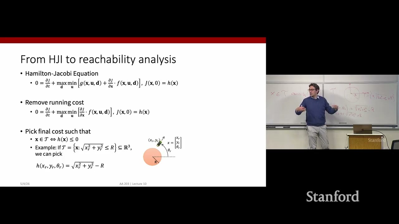
While the two-player structure matches the Hamilton-Jacobi-Isaacs formalism intuitively, a mathematical hurdle arises: standard optimal control formulations minimize or maximize an integrated cost function, whereas set membership is a binary condition (a state either lands inside the target set or it does not). To resolve this, Pavone introduces the **level set method**. The binary outcome can be completely embedded into the HJI formulation by making two critical structural modifications:
1. **Eliminate the running cost ($g \equiv 0$):** Because the only concern is whether the system state is inside or outside the target set at the terminal time $t = 0$, there is no intermediate running penalty along the path.
2. **Choose a terminal cost function ($h(x)$) whose zero sublevel set captures set membership:** The terminal cost $h(x)$ is constructed such that the target set $\mathcal{T}$ is precisely characterized by its zero level set.
Under this formulation, belonging to the target set $\mathcal{T}$ is equivalent to satisfying $h(x) \le 0$:
$$x \in \mathcal{T} \iff h(x) \le 0$$
[06:33](https://www.youtube.com/watch?v=3_gxaB_Pp3k&t=393s) Constructing the Level Set Function: A Geometric Example
To make the level set abstraction concrete, Pavone presents an intuitive geometric example using a unicycle model operating in a three-dimensional state space consisting of planar position coordinates and heading, $x = [x_r, y_r, \theta_r]^T$. Suppose the target set $\mathcal{T}$ is an obstacle defined as a circular disc of radius $R$ centered at the origin:
Pavone polls the class: if the unicycle is evaluated and $h(x) \le 0$, where is the vehicle located? A student responds that it is inside the circle. Pavone confirms: "Inside the circle. Exactly." The condition $h(x) \le 0$ means the Euclidean distance from the origin is strictly less than or equal to $R$. Conversely, if $h(x) > 0$, the system is safely outside the circular obstacle.
```mermaid
flowchart LR
accTitle: Level Set Function Mapping
accDescr: Representation of target set membership via the sign of the terminal cost function h(x).
Pavone highlights an elegant byproduct of this formulation:
- The sign of $h(x)$ encodes binary set inclusion.
- The magnitude of $h(x)$ quantifies safety margin. A large positive value of $h(x)$ indicates that the vehicle is far from danger, whereas an increasingly negative value indicates penetration deep inside the obstacle.
- In response to a student asking whether a larger positive value of $h$ always indicates higher safety, Pavone affirms: the magnitude provides a quantifiable "buffer" measuring how much room exists before crossing the zero boundary into danger.
[09:10](https://www.youtube.com/watch?v=3_gxaB_Pp3k&t=550s) Formulating the Hamilton-Jacobi-Isaacs Minimax Game for Avoidance and Reach Sets
With the running cost stripped out ($g = 0$) and the terminal cost $h(x)$ defined, avoidance and reachability problems map directly into the standard HJI partial differential equation framework. The boundary condition at final time $t = 0$ is governed purely by the terminal cost:
$$V(x, 0) = h(x)$$
For the **avoidance set** problem, Player 1 wants to prevent the system from entering the obstacle at $t = 0$, which corresponds to maximizing $h(x)$ to keep it positive. Nature (Player 2) acts adversarially to push the system into the obstacle, trying to force $h(x) \le 0$. This yields a minimax game:
$$\max_{u} \min_{d} \; h(x(0))$$
In contrast, when solving the **reach set** problem, Player 1 seeks to drive the system into the goal region ($h(x) \le 0$), while Player 2 attempts to prevent entry by making $h(x)$ positive. The game structure swaps players' roles, transforming the objective into a maximin game where Player 1 minimizes $h$ and Player 2 maximizes the cost:
$$\min_{u} \max_{d} \; h(x(0))$$
Pavone emphasizes that no new theoretical machinery is needed: by adjusting the order of the $\min$ and $\max$ operators and setting $g = 0$, both complex reachability problems can be proceduralized and resolved using standard HJI solvers.
[13:15](https://www.youtube.com/watch?v=3_gxaB_Pp3k&t=795s) From Backward Reachable Sets to Reachable Tubes
In zero-sum differential games, switching between reachability (reaching a target) and safety (avoiding a danger zone) corresponds directly to swapping the `min` and `max` operators in the terminal and Hamilton-Jacobi-Isaacs conditions. A student asks whether these definitions can be iterated to define a set that allows an agent to enter a feasible set. Pavone agrees that this is the essence of backward reachable sets: once a target set is established, the dynamics are propagated backward in time to determine the set of states from which one can reach or avoid that region.
However, Pavone points out a fundamental limitation of this formulation: it is essentially static with respect to trajectory execution. As initially structured, backward reachable sets (BRS) only evaluate whether the system ends up in an acceptable state at the final horizon endpoint ($t = 0$ in the backward time convention). In safety-critical autonomy, terminal safety alone is completely inadequate:
- Consider a safe trajectory whose endpoint at $t = 0$ lies outside the obstacle set, and whose entire history remains strictly outside; its cost function evaluation is positive, and it is correctly deemed safe.
- A collision trajectory ends up inside the obstacle set at $t = 0$, yielding a negative cost and being deemed unsafe.
- But consider an alarming edge case: a trajectory dips straight through an avoidance set at an intermediate time $\tau < 0$, but recovers and exits before $t = 0$. Because the cost only evaluates the state at $t = 0$, the endpoint cost remains positive, and the framework incorrectly classifies the path as "safe."
In an aviation context, passing through an avoidance zone during flight means having a near-miss or mid-air collision, even if the aircraft lands safely at the end of the trip. To protect an autonomous system along its entire trajectory rather than merely at the final time, one must generalize the backward reachable set into a **backward reachable tube (BRT)**.
[16:04](https://www.youtube.com/watch?v=3_gxaB_Pp3k&t=964s) Formulating the Hamilton-Jacobi-Isaacs Equation for Tubes
To enforce safety across the entire time horizon rather than at a single terminal time, the problem formulation replaces the terminal cost $h(x(0))$ with an infimum over all time:
$$\min_{\tau \in [t, 0]} h(x(\tau))$$
Requiring this minimum to be strictly positive guarantees that $h(x(\tau)) > 0$ at every single instant along the trajectory, meaning the vehicle never dips into the avoidance set.
```mermaid
flowchart LR
accTitle: Comparison of BRS and BRT Formulations
accDescr: Diagram contrasting Backward Reachable Set evaluating only terminal time versus Backward Reachable Tube evaluating the minimum cost across the full trajectory horizon.
subgraph BRS["Backward Reachable Set (BRS)"]
A["Terminal Cost: h(x(0))"] --> B["Evaluates safety only at final endpoint"]
end
subgraph BRT["Backward Reachable Tube (BRT)"]
C["Trajectory Infimum: min h(x(tau))"] --> D["Guarantees h(x(tau)) > 0 for all tau in horizon"]
end
```
Incorporating this running minimum changes the derivation of the Hamilton-Jacobi-Isaacs (HJI) PDE, introducing an extra minimization term into the dynamic programming operator. Pavone notes that while the resulting PDE is slightly more involved, the conceptual takeaway is clear: mathematical tools exist to compute safe reachable tubes over time horizons, and students can refer to the course citations for the explicit derivation.
When a student asks to clarify the distinction between solving for a BRS versus a BRT, Pavone explains that:
- A BRS identifies initial states that guarantee safety (or reachability) specifically at the endpoint of the optimization horizon.
- A BRT identifies the set of initial states that guarantee safety throughout the entire optimization horizon.
- In both cases, solving the HJI equation yields two essential outputs: the reachable set/tube itself (where the value function $V(t, x) > 0$) and the corresponding optimal feedback control policy $u^*(t, x)$.
If an agent starts in a safe state but fails to execute the minimax optimal control policy, disturbances or an adversarial agent can still push the system into the collision set. Once the value function is computed, evaluating the optimal control action at runtime requires only a straightforward gradient evaluation. When asked if tubes apply to target-reaching corridors, Pavone confirms that while mathematically possible, reachable tubes are overwhelmingly used in robotics and aerospace as safety buffers to avoid collisions. If the resulting safe set turns out to be empty, it indicates that the formulation is overly conservative or that the vehicle simply lacks sufficient control authority—a signal to either redefine the operational envelope or upgrade the actuators.
[22:37](https://www.youtube.com/watch?v=3_gxaB_Pp3k&t=1357s) Case Study: Aircraft Collision Avoidance with Unicycle Dynamics
To demonstrate practical HJI reachability, Pavone introduces a classic two-aircraft collision avoidance benchmark where both vehicles are modeled using unicycle kinematics in a 3D state space $(x, y, \theta)$:
$$\dot{x}_A = v \cos\theta_A, \quad \dot{y}_A = v \sin\theta_A, \quad \dot{\theta}_A = u_A$$
$$\dot{x}_B = v \cos\theta_B, \quad \dot{y}_B = v \sin\theta_B, \quad \dot{\theta}_B = u_B$$
Both aircraft travel at constant forward speed $v$ and steer by controlling heading rates through their angular inputs $u_A$ and $u_B$. Collision is defined as the relative distance between Aircraft A and Aircraft B falling below a critical safety radius $r$:
$$(x_A - x_B)^2 + (y_A - y_B)^2 \le r^2$$
Centering the coordinate frame on Aircraft A creates an avoidance zone of radius $r$ around player A. The objective is to identify the set of joint initial states $(x_A, y_A, \theta_A, x_B, y_B, \theta_B)$ from which Aircraft B—acting adversarially—can force a collision regardless of the evasive action chosen by Aircraft A.
Pavone emphasizes that this is not merely a theoretical toy example: "This is real stuff. I mean, how people may want to implement some level of collision avoidance for aircraft." He points out that he provided a companion reference implementation script for the course, enabling students to inspect the numerical grid-based reachability solver and see how the continuous HJI partial differential equation is solved to generate safety boundary tubes and evasion controls in practice.
[25:45](https://www.youtube.com/watch?v=3_gxaB_Pp3k&t=1545s) Hamilton-Jacobi Reachability for Aircraft Collision Avoidance
The discussion centers on a concrete collision avoidance problem formulated using differential game theory and solved via the Hamilton-Jacobi-Isaacs (HJI) partial differential equation. In this setup, the terminal avoidance set is defined as a circle with a radius of $5$ units, implemented through the terminal cost function $h$. The computation is performed using `hj_reachability`, an open-source Python package developed in Prof. Pavone’s lab.
The visualization produced by the solver is a three-dimensional surface representing the zero-level set of the value function $J$:
- $x$ denotes the relative longitudinal displacement between the two aircraft.
- $y$ denotes the relative lateral displacement.
- $z$ represents the relative heading between the vehicles.
The region where $J < 0$ (visualized as a green three-dimensional volume) corresponds to the set of initial relative states from which the opposing vehicle can force a collision despite optimal evasive action. If the initial state lies strictly outside this shape ($J \ge 0$), collision can be avoided.
When the relative heading is $z = 0$, both aircraft are flying parallel in the same direction. Under this condition, if they start outside the radius-5 circle, they can easily maintain separation indefinitely; if they start inside, they remain in a dangerous state. Consequently, at $z = 0$, the backward reachable set simply matches the circular shape of the baseline avoidance target.
```mermaid
flowchart TD
accTitle: HJI Collision Avoidance Problem Architecture
accDescr: Diagram illustrating relative coordinates fed into the HJI solver yielding a safe or collision outcome based on the zero-level set.
subgraph LevelSet["Zero-Level Set Outcome"]
JNeg["J < 0: Inside BRS<br/>(Potential Collision)"]
JPos["J >= 0: Outside BRS<br/>(Guaranteed Safe)"]
end
RelCoords --> PDE
Cost --> JNeg
Cost --> JPos
```
---
[28:22](https://www.youtube.com/watch?v=3_gxaB_Pp3k&t=1702s) Geometry of the Reachable Set Under Head-on Encounters
The geometry becomes asymmetrical and far more complex when the relative heading approaches $z \approx \pi$ (around $3$ radians), corresponding to a head-on encounter where the intruder aircraft is pointed directly toward the ego aircraft. Prof. Pavone struggles briefly with displaying the 3D model on the lecture projector, noting that interpreting the shape takes practice but quickly becomes intriguing once understood.
When the intruder aircraft is located with positive longitudinal displacement ahead of the ego vehicle and facing it, the backward reachable set protrudes significantly forward along the $x$-axis. Because the oncoming vehicle is directly closing the gap, the ego vehicle requires substantially more initial separation along the longitudinal axis to execute an evasive maneuver. Conversely, if the intruder is positioned behind the ego vehicle (negative longitudinal displacement) while facing opposite, it is simply flying away; the only requirement is that the vehicles do not already overlap inside the radius-5 avoidance circle at the start.
This pronounced protrusion—what Prof. Pavone affectionately calls a "blob"—directly captures the coupled kinematic and dynamic constraints of the Dubins-like aircraft model from first principles. When asked by a student whether the aircraft are assumed to share identical constant velocities, Prof. Pavone confirms that both travel at speed $v$, noting that assigning asymmetric velocities would warp the reachable set's geometry accordingly.
---
[31:43](https://www.youtube.com/watch?v=3_gxaB_Pp3k&t=1903s) 2D Projections, Horizon Length, and Steady-State Sets
To analyze the safety boundary more concretely, the 3D set is projected onto a 2D plane by fixing the relative heading at $z = 3.7$ radians (slightly greater than $\pi$). In this horizontal cross-section, dark blue contours designate the unsafe set ($J < 0$), bounded by a black zero-level curve.
Prof. Pavone poses an interactive question to the class to illustrate why the slice appears visibly tilted:
- If longitudinal separation is fixed at $x = 5$, should a pilot require a larger lateral buffer if the oncoming plane starts at a positive lateral distance or a negative lateral distance?
- Asking the students to vote between Option 1 and Option 2, the class unanimously selects the correct, intuitive option. Prof. Pavone jokes in response: "Great. Happy to fly with all of you."
- A positive lateral offset in this relative geometry forces the oncoming aircraft to perform a significantly more aggressive, complex turning maneuver to cause a collision, providing the ego vehicle ample time and room to evade. Thus, positive lateral positions require less protective margin, whereas negative lateral positions demand up to $5$ meters or more of lateral buffer, explaining the tilted geometry.
The backward reachable set also evolves back in time from the terminal horizon $t_f = 0$ toward negative values ($t = -2.5, -3.0, -3.5$). As the computation extends further back in time, the reachable set stabilizes. Beyond roughly $t = -3.5$ time units (e.g., at $t = -4, -5, -6$), the boundary ceases to expand and converges to a stationary set. In time-invariant differential games, once the initial transient clears, the game settles into a steady-state condition where the pursuer is permanently chasing or the encounter has already been decided; having additional time horizon available confers no further strategic advantage to either player.
---
[35:17](https://www.youtube.com/watch?v=3_gxaB_Pp3k&t=2117s) Trajectory Simulations, BRS vs. BRT, and Real-World Autopilot Systems
Prof. Pavone demonstrates the optimal closed-loop policies by simulating trajectories initialized inside and outside the backward reachable set, pitting Player 1 (ego, blue) against Player 2 (adversary/intruder, red):
1. **Initial state outside the set:** Player 2 aggressively maneuvers to intercept Player 1, but cannot breach the 5-unit personal space bubble. Both aircraft transition into a steady-state pursuit without collision.
2. **Initial state inside the set:** Player 2 starts within personal space, locks onto Player 1, and successfully maintains the collision state indefinitely.
3. **Transient boundary breach:** An edge case where Player 2 briefly enters Player 1's protected bubble during intermediate maneuvers before Player 1 manages to escape and pull away prior to the final time.
This third case reveals a critical theoretical nuance: under a standard Backward Reachable Set (BRS) formulation evaluated strictly at the terminal horizon, avoiding the bubble at $t = 0$ constitutes a mathematical success. In real safety-critical aviation, however, any transient violation of personal space is unacceptable. This limitation motivates using a **Backward Reachable Tube (BRT)** formulation, which tracks whether the state enters an unsafe set at *any* time instant across the entire trajectory $[t, 0]$, treating transient violations as definitive failures.
Prof. Pavone highlights that these theoretical tools are directly applied in industry. Several production-grade autonomous vehicle autopilots implement algorithms derived from backward reachability to enforce non-negotiable low-level safety envelopes, guaranteeing that an autonomous car maintains sufficient maneuvering buffer to avoid a crash regardless of erratic actions by surrounding drivers.
---
[38:18](https://www.youtube.com/watch?v=3_gxaB_Pp3k&t=2298s) Mathematical Wrap-Up and Computational Limits of PDE Solvers
In responding to a student question about convergence guarantees, Prof. Pavone clarifies that while they demonstrated a backward reachable set rather than a tube, time-invariant reachability formulations generally converge to well-defined steady-state solutions.
He acknowledges the steep theoretical curve of the material, calling differential games and HJI reachability "mathematically speaking, probably [...] the most sophisticated lecture" of the course. The primary practical obstacle to deploying HJI reachability broadly is the notorious curse of dimensionality associated with solving partial differential equations over dense grids:
- While his lab’s Python library (`hj_reachability`) provides one of the fastest implementations available, grid-based PDE solvers scale exponentially.
- In practice, standard HJI PDE techniques are computationally tractable only for state spaces up to 5 or 6 dimensions, necessitating alternative paradigms—such as Model Predictive Control—for high-dimensional systems.
[39:28](https://www.youtube.com/watch?v=3_gxaB_Pp3k&t=2368s) The Scalability Frontier in Reachability and the Transition to MPC
Exact Hamilton-Jacobi (HJ) reachability analysis suffers from the curse of dimensionality, typically hitting a hard computational wall around five or six state dimensions where grid-based PDE solvers cease to scale. While exact grid-based computation—such as that provided by tools like the `hj_reachability` package—breaks down beyond this threshold, solving higher-dimensional reachability problems is by no means impossible. Practitioners and researchers routinely circumvent the scalability barrier by adopting approximations, including sampling-based techniques and neural network representations, which trade formal worst-case accuracy guarantees for computational tractability.
```mermaid
flowchart TD
accTitle: Control Paradigms Comparison
accDescr: Diagram contrasting open-loop optimal control, closed-loop dynamic programming, and model predictive control.
subgraph Classical["Classical Extremes"]
OL["Open-Loop Optimal Control<br/>• Fast trajectory optimization<br/>• Vulnerable to disturbances"]
CL["Closed-Loop Optimal Control<br/>• Dynamic Programming / HJB / HJI<br/>• Robust feedback policy<br/>• Curse of dimensionality"]
end
subgraph SweetSpot["The Best of Both Worlds"]
MPC["Model Predictive Control (MPC)<br/>• Fast finite-horizon open-loop solves<br/>• Closed loop via receding horizon feedback"]
end
OL -->|"Combine speed with feedback"| MPC
CL -->|"Approximate infinite horizon tractably"| MPC
```
Turning away from dynamic programming and reachability, the lecture pivots to Model Predictive Control (MPC). Comparatively speaking, moving to MPC is "going to be a walk in the park in terms of complexity." Rather than wrestling with the mathematical intricacies of the continuous-time Hamilton-Jacobi-Bellman (HJB) or Hamilton-Jacobi-Isaacs (HJI) equations, MPC offers a paradigm that is profoundly intuitive and "just feels right" as a practical control strategy. Reflecting on the course roadmap:
- Open-loop optimal control is fast and computationally lightweight, but inherently fragile because it plans static sequences without feedback.
- Closed-loop optimal control (via the discrete-time Bellman equation or continuous HJB/HJI) produces robust feedback policies, but scales poorly due to prohibitive computational complexity.
- MPC bridges this gap, capturing the best of both worlds by uniting the computational efficiency of open-loop trajectory optimization with the robustness and adaptability of closed-loop feedback.
[41:39](https://www.youtube.com/watch?v=3_gxaB_Pp3k&t=2499s) Historical Origins and the Rise of MPC
MPC represents a broad framework rather than a rigid single algorithm. Second only to classical PID controllers, it stands as perhaps the most widely deployed control methodology in industry today. Its roots trace back to the 1970s and 1980s, when it emerged largely as an industrial heuristic within chemical engineering. Chemical processing proved to be the ideal proving ground for two specific reasons:
1. **Critical constraint satisfaction:** Chemical plants involve delicate reactions where operating parameters—most notably temperature—cannot be allowed to "go out of whack" without risking plant failure or catastrophic explosions. Classical frequency-domain linear control techniques could not handle hard state and actuator constraints directly.
2. **Slow physical timescales:** Unlike high-speed robotics or aerospace systems, chemical processes evolve sluggishly over intervals of multiple seconds. Even with the modest compute available in the 1970s and 1980s, solving constrained numerical optimization routines online at sample rates of 0.1 Hz to 0.5 Hz was entirely feasible.
Through the 1990s and 2000s, seminal contributions by researchers such as Francesco Borrelli, Alberto Bemporad, and Manfred Morari, alongside James B. Rawlings, David Q. Mayne, and Moritz Diehl, transformed MPC from an ad-hoc heuristic into a rigorous discipline grounded in mathematical stability and feasibility guarantees. Over subsequent decades, rapid advances in embedded processors and numerical convex optimization solvers have driven replanning rates from fractions of a hertz up to 10 Hz, 30 Hz, and even the kilohertz regime, pushing MPC into high-speed dynamic systems like autonomous driving, robotics, and aerospace.
[44:21](https://www.youtube.com/watch?v=3_gxaB_Pp3k&t=2661s) The Receding Horizon Philosophy
The fundamental premise of MPC addresses an infinite-horizon optimal control problem that is computationally intractable to solve globally in closed loop. MPC approximates this ideal by repeatedly solving a sequence of finite-horizon open-loop problems in discrete time.
```mermaid
flowchart LR
accTitle: Receding Horizon Control Loop
accDescr: Step-by-step cycle showing measurement, finite horizon optimization, input application, and horizon advancement.
A["Measure current state x(t)"] --> B["Solve finite-horizon open-loop problem over [t, t + N]"]
B --> C["Extract first input u*(t|t)"]
C --> D["Apply u*(t|t) to plant; discard remaining plan"]
D --> E["System transitions to x(t+1)"]
E -->|"Shift horizon to [t+1, t+1+N]"| A
```
At each discrete sampling instant $t$:
1. The controller measures or estimates the current system state $x_t$.
2. Conditioned on this state, system dynamics, and operating constraints, it formulates and solves an open-loop optimal control problem over a finite prediction horizon spanning from $t$ to $t + N_p$.
3. The optimization yields an optimal sequence of planned control inputs alongside the corresponding predicted state or output trajectory.
4. Crucially, the system applies **only the very first control action** in this computed sequence during the interval $[t, t+1)$.
5. The remainder of the planned trajectory is discarded.
6. As the physical plant transitions to state $x_{t+1}$, the planning horizon recedes forward by one step, and a fresh open-loop optimization is launched starting from the newly measured state $x_{t+1}$.
At first glance, discarding the rest of the planned sequence might seem wasteful. However, in practice, the discarded solution often warm-starts the numerical solver at the next tick. More importantly, this continuous replanning cycle is precisely what endows an open-loop solver with true closed-loop feedback characteristics: the optimization is continually re-anchored to real-world measurements, allowing the controller to reject unmodeled disturbances and modeling errors. This mimics human decision-making: a person plans out a walking path, takes a single step, gathers fresh visual and proprioceptive information, and immediately updates their plan.
[49:19](https://www.youtube.com/watch?v=3_gxaB_Pp3k&t=2959s) Discrete-Time Linear Constrained Formulation
To formalize the mathematical foundation, consider the regulation of a discrete-time linear time-invariant (LTI) system to the origin:
$$x_{t+1} = A x_t + B u_t$$
Unlike classical frequency-domain methods, MPC explicitly enforces state and actuator constraints:
where the admissible sets $\mathcal{X}$ and $\mathcal{U}$ are assumed to be polyhedra—geometric regions defined by the intersection of finitely many linear inequalities (such as hyperplanes forming bounding boxes or hypercubes).
Assuming full state measurement at time step $t$, the controller solves a constrained finite-horizon optimization problem over the control sequence $\{u_{t|t}, u_{t+1|t}, \dots, u_{t+N-1|t}\}$ to minimize an additive objective function:
Key structural aspects of this formulation include:
- **Double-index prediction notation:** The term $x_{t+k|t}$ denotes the state at future step $t+k$ predicted from the perspective of sampling time $t$, and $u_{t+k|t}$ represents the planned input for that step. The distinction matters because external disturbances or model mismatch mean that $x_{3|1}$ (the state predicted for step 3 when planning at step 1) will rarely match $x_{3|2}$ (the state predicted for step 3 when re-evaluating at step 2).
- **Initial condition anchoring:** Setting $x_{t|t} = x_t$ ties the mathematical optimization directly to the actual state measurement at run time, injecting feedback into the loop.
- **Terminal ingredients:** The formulation introduces both a terminal cost $\ell_f(x_{t+N|t})$ and a terminal constraint set $\mathcal{X}_f$. These components act as crucial theoretical anchors to ensure stability and recursive feasibility across subsequent replanning steps.
[52:42](https://www.youtube.com/watch?v=3_gxaB_Pp3k&t=3162s) The MPC Tuning Knobs and Core Objectives
When constructing an optimal control formulation for Model Predictive Control (MPC), standard components like stage (running) costs and control constraints are familiar, but two specialized ingredients are introduced to regularize the formulation: a terminal constraint set and an auxiliary terminal cost penalizing the predicted state at horizon $N$. These elements are not arbitrary mathematical artifacts; they serve as the primary design choices and "tuning knobs" available to control engineers to shape closed-loop behavior, ensure numerical tractability, and guarantee performance upon deployment. Alongside the terminal cost and terminal constraint set, the prediction horizon length $N$ constitutes the third fundamental tuning knob.
```mermaid
flowchart TD
accTitle: Online MPC Receding Horizon Loop
accDescr: Flowchart illustrating the online execution cycle of Model Predictive Control from state measurement to control application.
subgraph SenseAndSolve["1. State Observation & Optimization"]
A["Measure current state x(t)"] --> B["Solve finite-horizon OCP over horizon N"]
end
subgraph FeasibilityCheck["2. Feasibility Evaluation"]
B --> C{"Is problem feasible?"}
C -->|"No"| D["Infeasible: Stuck / Call for help"]
C -->|"Yes"| E["Extract optimal sequence {u_0*,..., u_{N-1}*}"]
end
subgraph ActuateAndAdvance["3. Receding Horizon Execution"]
E --> F["Apply first control input u_0* to system"]
F --> G["System evolves to state x(t+1)"]
G -->|"Advance t to t+1"| A
end
```
Whenever deploying an MPC framework, system designers prioritize two fundamental properties above all else:
- **Persistent Feasibility:** The controller must guarantee that whenever the system transitions to a successor state, the freshly instantiated optimal control problem remains feasible. If the reachable set becomes empty, the optimization solver fails, leaving the system stranded with no admissible action that avoids constraint violation.
- **Stability and Task Fulfillment:** Assuming persistent feasibility holds, the resulting closed-loop system must successfully regulate the state to the target set or equilibrium—most commonly driving the state to the origin ($x \to 0$).
---
[54:53](https://www.youtube.com/watch?v=3_gxaB_Pp3k&t=3293s) Receding Horizon Feedback and Horizon Length Tradeoffs
The conceptual bridge connecting open-loop optimal control trajectories to a true closed-loop feedback policy lies in the receding horizon mechanism. At each sampling instant $t$, an open-loop optimal control problem is solved over the lookahead horizon using the measured physical state $x_t$ as the initial condition. From the resulting optimal control trajectory, only the very first control action $u_0^*(x_t)$ is applied to the physical plant. At the next time step $t+1$, the system measures the updated state $x_{t+1}$, shifts the horizon forward, and resolves the optimization problem anew. Defining the policy $\pi(x_t) = u_0^*(x_t)$ yields the closed-loop system dynamics:
$$x_{t+1} = A x_t + B \pi(x_t) = f_{\text{cl}}(x_t)$$
In time-invariant settings—where system matrices $A$, $B$, and constraint sets do not vary with absolute time—the cumbersome double-indexing notation (tracking predictions made at time $t$ for future time $t+k$) can be streamlined. One simply formulates a standard optimization starting from an initial condition $x_0 = x_t$, applies $u_0$, observes the transition to $x_{t+1}$, and repeats the procedure with $x_0 = x_{t+1}$.
In response to a student question regarding whether the prediction horizon $N$ must be sufficiently long to reach the terminal set, horizon selection represents an approximation of an underlying infinite-horizon problem. Horizon length imposes a direct engineering trade-off:
- **Overly Short Horizons:** If $N$ is too short, the controller becomes myopic or excessively aggressive. In severe cases, a myopic controller may fail to converge, render the state unable to reach the terminal target, or drive the system into an inescapable constraint-violating corner.
- **Longer Horizons:** Increasing $N$ expands the lookahead horizon, improving stability, constraint satisfaction, and convergence margins ("in general, the longer the better").
- **Computational Overhead:** Longer horizons significantly increase the dimensionality of the mathematical program, escalating online solver latency. The designer must delicately balance real-time computational budgets against task completion and convergence guarantees.
---
[01:00:24](https://www.youtube.com/watch?v=3_gxaB_Pp3k&t=3624s) The Online MPC Algorithm and Historical Perspective
In practical applications, MPC stage costs commonly adopt quadratic penalties analogous to Linear Quadratic Regulator (LQR) designs, penalizing state and control deviations via positive semi-definite and positive definite weighting matrices. Alternatively, designers employ $p$-norms such as the 1-norm (summing the absolute values of vector components) or the infinity-norm (taking the maximum component magnitude), both of which yield linear programming formulations that facilitate efficient real-time solving.
```
Algorithm: Standard Online Model Predictive Control
1. Measure the current physical state x(t).
2. Formulate and solve the finite-horizon optimal control problem starting at x(t).
3. If the solver reports infeasibility:
System is trapped; trigger safety fallback ("call for help").
Else:
Extract optimal sequence and apply the first control u_0 to the system.
4. Allow system to transition to x(t+1).
5. Increment t ← t + 1 and repeat from Step 1.
```
While explicit or offline MPC approaches compute look-up tables of parametric solutions offline across all anticipated initial states, standard practice focuses predominantly on this online receding horizon cycle.
From a historical vantage point, selecting the tuning parameters ($N$, terminal cost $p(\cdot)$, and terminal set $X_f$) remained largely an empirical, heuristic art throughout the industrial adoptions of the 1970s and 1980s. Between the 1990s and the 2000s, control theorists introduced rigorous analytical frameworks to replace trial-and-error tuning. Direct closed-loop analysis of $x_{t+1} = f_{\text{cl}}(x_t)$ proved excessively intractable because the vector field $f_{\text{cl}}$ is an implicit, nonlinear mapping defined by the solution of a constrained optimization problem. The breakthrough emerged when researchers realized they could synthesize structural conditions directly onto the terminal cost and terminal constraint set, guaranteeing persistent feasibility and Lyapunov stability *by design* without needing to simulate or inspect individual closed-loop trajectories beforehand.
---
[01:03:45](https://www.youtube.com/watch?v=3_gxaB_Pp3k&t=3825s) Invariant Set Theory: Feasible and Controllable Sets
To establish persistent feasibility on rigorous theoretical footing, modern MPC leverages tools from invariant set theory. While slightly heavy on geometric definitions, invariant set theory provides the exact mathematical language required to prevent controller failure.
The analysis begins by establishing two fundamental sets:
- **Set of Feasible Initial States ($X_0$):** Defined as the set of all current states $x \in X$ for which there exists at least one admissible control sequence $\{u_0, u_1, \dots, u_{N-1}\} \subseteq U$ such that the resulting state trajectory satisfies all intermediate state constraints ($x_k \in X$ for all $k = 0, \dots, N-1$) and terminates strictly within the designated terminal set ($x_N \in X_f$). The MPC optimization problem admits a valid solution if and only if the current state belongs to $X_0$.
- **One-Step Controllable Set:** For a discrete-time autonomous system subject to state and input bounds, the one-step controllable set to a target set $S$ comprises all states in the state space from which there exists a feasible control input that propels the system into $S$ on the very next time step while respecting system constraints.
Characterizing these backward reachable regions enables control designers to configure the terminal constraint set $X_f$ so that steering the predicted trajectory into $X_f$ at step $N$ inherently guarantees the existence of a feasible continuation trajectory at step $N+1$.
[01:06:13](https://www.youtube.com/watch?v=3_gxaB_Pp3k&t=3973s) One-Step Controllable Sets and Control Invariance
To build up the formal machinery for persistent feasibility in Model Predictive Control (MPC), the discussion introduces set-theoretic definitions starting with the predecessor set, or one-step controllable set. For an autonomous dynamical system $x_{t+1} = f(x_t)$, the predecessor set $\text{Pre}(S)$ (or previous set of $S$) answers the fundamental question: what is the set of initial states such that taking one step under the natural system dynamics lands you inside $S$?
```mermaid
flowchart LR
accTitle: Predecessor and Control Invariant Set Transitions
accDescr: Visual flow showing states transitioning into set S or remaining in set C via control input u.
subgraph PreSet["Predecessor Set: Pre(S)"]
XPre["x in Pre(S)"] -->|"f(x, u) with u in U"| TargetS["Next state in S"]
end
subgraph InvariantSet["Control Invariant Set: C"]
XC["x_t in C"] -->|"exists u such that f(x_t, u)"| NextC["x_{t+1} in C"]
end
```
This definition generalizes directly to controlled systems $x_{t+1} = f(x_t, u_t)$. For a controlled system, the one-step controllable set $\text{Pre}(S)$ is defined as the set of states for which there exists an admissible control input $u$ such that the one-step transition $f(x, u)$ lands directly into $S$.
This leads directly into the ubiquitous MPC concept of a control invariant set:
- A set $\mathcal{C}$ is a **control invariant set** for a system $x_{t+1} = f(x_t, u_t)$ if, whenever the current state $x_t \in \mathcal{C}$, there exists an admissible control $u_t$ such that the successor state $x_{t+1} = f(x_t, u_t)$ remains inside $\mathcal{C}$. Intuitively, think of $\mathcal{C}$ as a "safe set" where the system remains sufficiently far from danger, and there always exists a control action that keeps it there.
- The **maximal control invariant set**, denoted $\mathcal{C}_\infty$, is the largest possible control invariant set for the dynamical system—meaning it contains all other control invariant sets.
- For an autonomous system without explicit input dependency, the analogous property is called **positive invariance**: if $x_t \in A$, then $f(x_t) \in A$.
- Computationally, these geometric polyhedral sets can be calculated using the Multi-Parametric Toolbox (MPT) in MATLAB, which students will use in their homework assignments.
[01:09:51](https://www.youtube.com/watch?v=3_gxaB_Pp3k&t=4191s) Maximal vs. Non-Maximal Invariant Sets
A student asks for clarification on how a control invariant set could fail to be maximal, requesting an intuitive example of a non-maximal set.
The canonical example is a single equilibrium point, such as the origin $\{0\}$ for a linear system $x_{t+1} = Ax_t + Bu_t$. If the system starts at $x = 0$ and $u = 0$ is a feasible control input, the next state is $A(0) + B(0) = 0$. Thus, the singleton set containing only the origin satisfies the definition of being control invariant because you can remain there indefinitely. However, it is obviously not maximal—there are typically many other states outside the origin from which the system can still transition and remain within some larger invariant region.
[01:11:05](https://www.youtube.com/watch?v=3_gxaB_Pp3k&t=4265s) Truncated Feasibility and Persistent Feasibility Lemma
Connecting these set concepts back to MPC feasibility requires defining the truncated feasibility set, denoted $X_1$. This is the set of states for which the optimal control problem is feasible over a shortened horizon of length $N - 1$. More precisely, it is the set of states for which there exists a truncated control sequence starting from time step 1 rather than time step 0 (i.e., sequence $\{u_1, \dots, u_{N-1}\}$ with $u_k \in \mathcal{U}$) such that the resulting state trajectory satisfies all state constraints as well as the terminal constraint $x_N \in X_f$.
The foundational result linking invariance to feasibility is established:
- **Lemma:** If the truncated feasibility set $X_1$ is a control invariant set for the system, then the receding-horizon MPC control law is guaranteed to be **persistently feasible**.
- The core intuition is that if $X_1$ is control invariant, you can use that invariant property to "buy a one-step of staying in that set" at the current time, and then execute the feasible solution for the remaining $N - 1$ steps.
- On its own, this lemma is practically unusable because $X_1$ is an implicit construct rather than an explicit tuning knob. The system designer directly tunes the terminal cost matrix $P$, the terminal constraint set $X_f$, and the horizon length $N$, but cannot directly tune $X_1$.
- Nevertheless, the lemma is the essential theoretical stepping stone needed to derive actionable theorems that provide explicit recipes for choosing $P$ and $X_f$ to guarantee both persistent feasibility and closed-loop asymptotic stability. The proof of this lemma and the resulting stability theorems will be completed in the following lecture and applied in the problem set.
## Notable quotes
> [06:33](https://www.youtube.com/watch?v=3_gxaB_Pp3k&t=393s) Inside the circle. Exactly. — Prof. Marco Pavone
> [22:37](https://www.youtube.com/watch?v=3_gxaB_Pp3k&t=1357s) This is real stuff. I mean, how people may want to implement some level of collision avoidance for aircraft. — Prof. Marco Pavone
> [31:43](https://www.youtube.com/watch?v=3_gxaB_Pp3k&t=1903s) Great. Happy to fly with all of you. — Prof. Marco Pavone
> [38:18](https://www.youtube.com/watch?v=3_gxaB_Pp3k&t=2298s) mathematically speaking, probably [...] the most sophisticated lecture — Prof. Marco Pavone
> [39:28](https://www.youtube.com/watch?v=3_gxaB_Pp3k&t=2368s) going to be a walk in the park in terms of complexity. — Prof. Marco Pavone
> [39:28](https://www.youtube.com/watch?v=3_gxaB_Pp3k&t=2368s) just feels right — Prof. Marco Pavone
> [41:39](https://www.youtube.com/watch?v=3_gxaB_Pp3k&t=2499s) go out of whack — Prof. Marco Pavone
> [54:53](https://www.youtube.com/watch?v=3_gxaB_Pp3k&t=3293s) in general, the longer the better — Prof. Marco Pavone
> [01:00:24](https://www.youtube.com/watch?v=3_gxaB_Pp3k&t=3624s) call for help — Prof. Marco Pavone
> [01:11:05](https://www.youtube.com/watch?v=3_gxaB_Pp3k&t=4265s) buy a one-step of staying in that set — Prof. Marco Pavone
## Mentioned
Prof. Marco Pavone, Dr. Daniele Gammelli, Stanford University, NVIDIA, NASA Jet Propulsion Laboratory, Principles of Robot Autonomy, Hamilton-Jacobi-Isaacs (HJI) equation, Hamilton-Jacobi-Bellman (HJB) equation, Model Predictive Control (MPC), hj_reachability, Francesco Borrelli, Alberto Bemporad, Manfred Morari, James B. Rawlings, David Q. Mayne, Moritz Diehl, Linear Quadratic Regulator (LQR), Multi-Parametric Toolbox (MPT), MATLAB, Dubins car model, PID controller
## Video description
Lecture 11 — Introduction to Model Predictive Control
Read the companion textbook, Principles of Robot Autonomy, free online: https://porabook.com
To learn more about enrolling in AA203 Optimal and Learning-Based Control, visit: https://online.stanford.edu/courses/aa203-optimal-and-learning-based-control
Follow along with the course schedule and syllabus: https://stanfordasl.github.io/aa203/sp2526/
Bio: Dr. Marco Pavone is an Associate Professor of Aeronautics and Astronautics at Stanford University and a Senior Director of Autonomous Vehicle Research at NVIDIA. Prior to joining Stanford, he was a Research Technologist in the Robotics Section at NASA’s Jet Propulsion Laboratory. Dr. Pavone received his Ph.D. in Aeronautics and Astronautics from the Massachusetts Institute of Technology in 2010. His research focuses on the analysis, design, and control of autonomous systems, with particular emphasis on self-driving cars, autonomous aerospace vehicles, and future mobility systems. He has been recognized with numerous awards, including the Presidential Early Career Award for Scientists and Engineers from President Barack Obama, the Office of Naval Research Young Investigator Award, the NSF CAREER Award, the NASA Early Career Faculty Award, the IEEE Kiyo Tomiyasu Award, the CSS Award for Technical Excellence in Aerospace Control, and the Early-Career Spotlight Award from the Robotics Science and Systems Foundation.
Instructors:
Prof. Marco Pavone, Associate Professor of Aeronautics and Astronautics, Director of Autonomous Vehicle Research at NVIDIA
Dr. Daniele Gammelli, Research Director at the Italian Institute of Artificial Intelligence (AI4I), Researcher at the Department of Aeronautics and Astronautics, Stanford University
Full playlist: https://www.youtube.com/playlist?list=PLa9dmHsLK9dg
Professor Marco Pavone outlines the mathematical transition from continuous-time Hamilton-Jacobi reachability analysis to discrete-time Model Predictive Control (MPC), balancing computational tractability against safety and stability guarantees.
Hamilton-Jacobi Reachability and Continuous Trajectory Safety (0:05)
Reachability theory frames safety verification as a zero-sum differential game resolved via the Hamilton-Jacobi-Isaacs (HJI) partial differential equation. Using the level set method, the running cost is eliminated ($g \equiv 0$) and target set membership is embedded into a terminal cost $h(x) \le 0$, where the sign indicates inclusion and the magnitude quantifies safety margin. However, evaluating Backward Reachable Sets (BRS) strictly at the terminal horizon $t = 0$ creates a critical vulnerability: trajectories that breach an obstacle set at an intermediate time before recovering are misclassified as safe.
To ensure continuous safety over a mission, the formulation extends to Backward Reachable Tubes (BRT) by evaluating the infimum over time, $\min_{\tau \in [t, 0]} h(x(\tau)) > 0$. Pavone illustrates this with a two-aircraft collision avoidance problem using unicycle dynamics and a 5-unit separation radius solved via `hj_reachability`. Under head-on encounters, the required safety boundary protrudes significantly along the longitudinal axis, showing how kinematic limits dictate protective margins and how tube formulations prevent transient near-misses.
Computational Scalability Bottlenecks and the MPC Alternative (39:28)
Exact grid-based HJI reachability provides robust worst-case policies but encounters a strict computational barrier: the curse of dimensionality limits dense PDE solvers to systems with five or six state dimensions. While practitioners employ approximations like sampling or neural networks for higher dimensions, Model Predictive Control emerges as the predominant framework to handle constrained, high-dimensional dynamics.
Historically developed in the 1970s and 1980s for slow-moving chemical processes operating at 0.1–0.5 Hz, MPC was formalized through the 1990s and 2000s into a mathematically rigorous discipline. Faster processors and convex solvers now enable replanning rates up to kilohertz frequencies. Pavone highlights that MPC unites the speed of open-loop trajectory optimization with the disturbance rejection of closed-loop feedback, avoiding the exponential intractability of dynamic programming.
Receding Horizon Control and Optimization Design Knobs (44:21)
Rather than attempting an intractable infinite-horizon closed-loop solve, MPC repeatedly computes finite-horizon open-loop problems across discrete steps. At each sampling instant $t$, the system measures state $x_t$ and solves a constrained optimization problem over horizon $N$, enforcing system dynamics alongside polyhedral state and actuator constraints ($x \in \mathcal{X}, u \in \mathcal{U}$). The system executes only the first planned input $u_0^*$, discards the remaining sequence, and advances the horizon, continually re-anchoring predictions to physical measurements.
System designers tune three primary parameters: the prediction horizon length $N$, the terminal constraint set $\mathcal{X}_f$, and the terminal cost $\ell_f(x_{t+N|t})$. Horizon length presents a fundamental engineering trade-off: short horizons risk myopic behavior, infeasibility, or failure to converge, whereas longer horizons expand stability margins at the expense of higher online computational latency.
Invariant Set Theory and Guarantees of Persistent Feasibility (63:45)
Deploying online MPC requires preventing solver infeasibility, which leaves autonomous systems stranded without an admissible control action. Because analyzing the closed-loop dynamics $x_{t+1} = f_{\text{cl}}(x_t)$ directly is intractable due to the implicit, nonlinear optimization mapping, modern control leverages invariant set theory to guarantee feasibility and Lyapunov stability by design.
A set $\mathcal{C}$ is defined as control invariant if every state in $\mathcal{C}$ possesses an admissible control input whose one-step transition remains within $\mathcal{C}$. Pavone introduces a foundational lemma: if the truncated feasibility set $X_1$ (the set of states feasible over a reduced horizon $N-1$) is control invariant, the receding-horizon control law is guaranteed to remain persistently feasible. Because $X_1$ is an implicit construct rather than a directly tunable parameter, this lemma serves as the theoretical bridge for deriving explicit synthesis conditions on the terminal set $\mathcal{X}_f$ and terminal cost.
While MPC circumvents the dimensional limits of continuous dynamic programming by solving constrained open-loop programs online, ensuring that the controller never encounters infeasibility requires rigorous terminal constraints. The primary unresolved task is translating implicit invariance conditions on truncated feasibility into explicit design recipes for terminal sets and terminal costs.
Source quotes
[6:33] Prof. Marco Pavone: Inside the circle. Exactly.
[22:37] Prof. Marco Pavone: This is real stuff. I mean, how people may want to implement some level of collision avoidance for aircraft.
[31:43] Prof. Marco Pavone: Great. Happy to fly with all of you.
[38:18] Prof. Marco Pavone: mathematically speaking, probably [...] the most sophisticated lecture
[39:28] Prof. Marco Pavone: going to be a walk in the park in terms of complexity.
[39:28] Prof. Marco Pavone: just feels right
[41:39] Prof. Marco Pavone: go out of whack
[54:53] Prof. Marco Pavone: in general, the longer the better
[60:24] Prof. Marco Pavone: call for help
[71:05] Prof. Marco Pavone: buy a one-step of staying in that set
Original transcript
[0:05] So today, we're going to
continue our discussion
[0:08] about reachability,
and then we move
[0:10] on to the next
topic, which is that
[0:12] of model predictive control.
[0:15] So as you remember
from last time,
[0:17] we discussed how a
particularly useful application
[0:21] of continuous time
closed-loop optimal control
[0:25] is represented by
reachability theory.
[0:28] That essentially involves
computing reachable sets
[0:33] through the lens of the
Hamilton-Jacobi-Isaacs equation.
[0:36] So we discussed last time
what reachable sets are
[0:40] and what they represent.
[0:41] Depending on the interpretation
for the target set,
[0:45] we have two main instantiations
of the concept of reachable set,
[0:49] namely avoidance
set and reach sets.
[0:54] So what we're going to do today
is, based on these definitions,
[0:58] see how we can apply the
Hamilton-Jacobi-Isaacs
[1:01] equation to compute these
mathematical objects.
[1:04] And then I will
discuss how, once you
[1:06] have computed these
objects, you could use
[1:08] those in a control pipeline.
[1:13] Any questions?
[1:15] So just as a reminder, we
defined an avoidance set,
[1:23] which is a particular
instantiation of a backward
[1:26] reachable set, as the
set of states at time, t,
[1:29] satisfying the
following definition.
[1:33] A stands for avoidance.
[1:36] This is the set of states for
which there exists a disturbance
[1:39] such that for all
possible control,
[1:41] the system enters the target
set at time t equal 0.
[1:47] And of course, once you
have computed this set,
[1:49] you want to make sure that
you start outside of this set
[1:53] to guarantee safety.
[1:55] For the opposite, the
reachable set is actually
[1:59] the set of desirable
states, and is
[2:01] defined as the set
of states at time, t,
[2:05] such that for all
disturbances, there
[2:07] exists a control such
that the system enters
[2:09] target set at time t equals 0.
[2:12] So in this case, you would like
to start within this set so that
[2:17] no matter what nature
throws at you that there
[2:19] is a control, the optimal
control, that will still
[2:22] allow you to fulfill
your control objectives.
[2:26] So this naturally
become a constraint
[2:28] in your trajectory
optimization problem.
[2:30] You want to ensure that in
the case of avoidance set,
[2:34] your trajectory stays
outside of that set.
[2:36] In the case of a
reach set, you want
[2:40] to make sure that your initial
condition is within that set.
[2:47] Now the question is, how
we compute these sets?
[2:50] So the point is that you can
use the Hamilton-Jacobi-Isaacs
[2:55] equation to compute these
sets in a very procedural way.
[3:00] Specifically, as we will
see, the computation
[3:03] of the backward reachable
sets, both in the avoidance
[3:05] case and the reach case, entails
solving a differential game
[3:09] where the outcome is Boolean.
[3:11] What does it mean a
differential game?
[3:13] From last time,
differential game
[3:15] means that there
are two players.
[3:17] We are player 1.
[3:18] We use the controls
at our disposal
[3:21] in order to either
avoid a target set
[3:25] or reach a target set.
[3:26] And then there is
player 2, nature,
[3:29] that, through a
disturbance control,
[3:31] is trying to thwart our
attempt to fulfill our control
[3:35] objectives.
[3:38] Now, the question is, at
the level of a two-player
[3:42] structure--
[3:43] should be quite
intuitive that, actually,
[3:45] the Hamilton-Jacobi-Isaacs
formalism is well set up
[3:47] to address these problems.
[3:49] The question, though, how do
we instantiate all the problem
[3:53] formulation in a
way that is aligned
[3:56] with the definition of
backward reachable set,
[3:58] particularly because
belonging to a set
[4:02] or not is a binary condition?
[4:06] When backward reachable set--
sorry, in the optimal control
[4:10] formulation, we only framed it
in terms of a cost function.
[4:14] So the question is, can we
reframe membership to a set
[4:22] through the lens
of a cost function
[4:24] so that we can reduce everything
to the optimal control
[4:26] formulation, to
which we can then
[4:28] apply the
Hamilton-Jacobi-Isaacs equation?
[4:31] And the short answer is, yes, we
can encode this Boolean outcome
[4:36] of belonging or
not to target set
[4:40] within the
Hamilton-Jacobi-Isaacs
[4:42] formulation by removing
the running cost.
[4:45] Since we only care about
being in the target
[4:48] set at the final time or
not being in the final set
[4:51] at the target time, there is
no notion of running cost.
[4:56] And by picking the final cost,
to denote set membership.
[5:01] The question is how we do that?
[5:03] It turns out that this
is relatively easy
[5:07] and leads to the level
set method for backward
[5:12] reachable computations.
[5:15] Specifically,
remember the equations
[5:18] that one needs to solve in order
to find the optimal control
[5:22] profile in a differential game.
[5:27] In our problem, we
only care about getting
[5:30] into the backward reachable
set at the final time.
[5:34] There is no notion
of a running cost.
[5:36] So accordingly, we set the
running cost, g, equal to 0
[5:40] for the specific
case of computing
[5:43] backward reachable set.
[5:45] So we are only left
with the final cost, h,
[5:49] which shows up in the
boundary condition
[5:51] for the partial
differential equation.
[5:53] Now, can we pick a final
cost that reflects the notion
[5:59] that you either
belong to a target set
[6:01] or you do not belong
to the target set?
[6:04] And the answer is affirmative.
[6:06] So one can always
find a function h
[6:09] of x such that set
t, the target set,
[6:14] is equal to the
0 level set of h.
[6:17] That is, x belongs to a given
set t if and only if h of x
[6:28] is less than or equal to 0.
[6:33] Let me give you an example.
[6:34] And through the example, you
see that this is actually
[6:36] quite obvious.
[6:37] So let's assume that
the set, capital T,
[6:40] is represented by a
circle with radius R.
[6:48] So T is defined as
the set of point
[6:54] x such that x squared plus
y squared is less than
[7:02] or equal to R.
[7:07] Now, you can define
a function h that
[7:11] is a function of--
so let's assume
[7:13] that the state space of our
system is three-dimensional.
[7:15] So we have a unicycle
with state x.
[7:18] The longitudinal position
y, the lateral position.
[7:21] And theta, the heading.
[7:23] So we can define the function
h as h of xr yr theta r
[7:30] as square root of--
[7:42] so if your unicycle,
whose state space
[7:47] is three-dimensional, x, y
position and heading, has xy
[7:53] coordinates such that h is
negative, what is the unicycle?
[7:58] We assume that we have a
reference frame like this one.
[8:07] If the function h is less than
or equal to 0, what is it?
[8:12] Inside the circle.
[8:13] Inside the circle.
[8:14] Exactly.
[8:15] Because it means that the
distance is less than R.
[8:20] So if h less than or
equal to 0, it means--
[8:25] x squared plus y
squared less than
[8:27] or equal to R, which means that
its position, its displacement
[8:32] from the origin, has
to be less than R.
[8:34] So it's inside the circle.
[8:36] If h is greater than 0, it
means that you are outside.
[8:40] And of course, the more h
is negative means the deeper
[8:44] you are in the circle.
[8:45] The more h is positive, the
farther you are from the circle.
[8:50] Actually, the magnitude h
also has an interpretation
[8:53] in terms of how safe
or how unsafe you are.
[8:57] But most importantly,
the level set of h
[9:03] tells you whether a system
is in the target set
[9:07] or is not in the target set.
[9:10] So then the idea of reframing
backward reachable set
[9:14] through the lens of
Hamilton-Jacobi-Isaacs equation
[9:16] is fairly straightforward.
[9:17] You remove the running cost.
[9:19] This is not a notion
on running cost.
[9:20] In computing backward
reachable sets,
[9:22] you find a function
h that represents
[9:26] belonging to a given set
for whatever target set, t,
[9:31] you have defined.
[9:32] That's always possible.
[9:34] Of course, if you have something
that is a bit more complicated
[9:37] than a circle, then
a function h is
[9:39] going to be a bit
more complicated,
[9:40] but that's not a problem.
[9:44] And thus, we have
reframed the problem
[9:48] of avoidance of a target set
as the problem of maximizing
[9:56] over u.
[9:56] We want to stay
outside of the set.
[9:59] So we want to make--
[10:00] us, as player 1, we
want to make h positive
[10:03] while the enemy, player 2,
wants to make h negative.
[10:07] And so we are in the
same exact formalism
[10:10] of the Hamilton-Jacobi-Isaacs
problem,
[10:13] but the difference is that
we only have the final cost.
[10:16] We don't have the running cost.
[10:19] Remember that for the
continuous time optimal control
[10:22] formulation, the
final time is 0.
[10:24] So we start from some negative
time and the final time is 0.
[10:27] This is more of a convention.
[10:30] So this is an example.
[10:31] So this is an example
where the avoidance
[10:33] set is this red circle.
[10:38] For this trajectory
here, the cost
[10:42] is positive since
the final point
[10:46] is outside of the
avoidance set, which
[10:47] means that the h, the
final cost, is positive.
[10:51] And then opposite to that,
for this blue trajectory,
[10:56] the final condition is
in the circle, which
[10:58] means that h is negative, which
means that the overall cost is
[11:03] negative.
[11:05] So we're not doing
anything deep here.
[11:07] We're just trying to find
a one-to-one correspondence
[11:10] between the abstract problem
of backward reachable set
[11:12] computation and the tool
that we know of, which is
[11:15] that of Hamilton-Jacobi-Isaacs.
[11:16] Yeah.
[11:17] [INAUDIBLE] show me how
safe you are? [? Will h ?]
[11:21] always be more positive?
[11:23] Yeah, yeah.
[11:23] So that's why, actually,
the magnitude of h
[11:27] not only allows you to reflect
the problem of a reachable set
[11:31] computation in the
Hamilton-Jacobi-Bellman
[11:33] framework, but also gives you
some interesting additional
[11:36] information, which is,
loosely speaking, a buffer.
[11:39] The information about
how much buffer you
[11:41] have before crossing
the danger line,
[11:44] which is when h is equal to 0.
[11:45] So short answer is yes.
[11:48] OK, so we're almost there.
[11:52] So this is the formulation
for an avoidance set.
[11:56] So now that you want to--
[11:58] so if you have a
problem where you
[12:00] want to find a backward
reachable set, that is,
[12:03] the set of initial conditions
that would lead you
[12:06] to a collision-- so for your
set to enter some unsafe region
[12:11] for some adversarial selection
of the [INAUDIBLE] profile,
[12:16] the problem that you want
to solve is minimax problem.
[12:20] We already discussed
how to pick h.
[12:23] And then there is nothing
else that you have to do.
[12:25] You just write down the
Hamilton-Jacobi-Isaacs equation
[12:29] for this specific problem.
[12:31] Same as last time.
[12:33] We don't have the running cost.
[12:35] And of course, for the
boundary condition,
[12:37] we use the h function
that represents membership
[12:40] to a given set.
[12:42] If instead you want to solve
the opposite problem, that
[12:45] of reaching a goal-- so now
you want to enter into the set.
[12:49] So you want to make h negative.
[12:51] And the player wants to
make-- the nature wants
[12:54] to make h positive
because it doesn't
[12:56] want you to go into the set.
[12:59] Then the problem formulation
is a swap in terms of minimax.
[13:03] And now, you want to minimize h.
[13:06] Player 2 wants to
maximize the cost.
[13:11] So all stays the same.
[13:12] It's just that the
max min and min max
[13:15] are swapped in the conditions.
[13:17] So you would do the
same derivation,
[13:19] but just swapping min max.
[13:21] Yeah.
[13:22] [INAUDIBLE] would
like to be used
[13:24] to define a set such that you
can enter the feasible set?
[13:27] Like iterate?
[13:30] A set--
[13:31] If you got reachable sets.
[13:37] Right?
[13:38] Yeah, I mean that's the notion
of backward reachable set.
[13:40] But by feasible set,
what do you mean exactly?
[13:43] [INAUDIBLE] course.
[13:45] Yeah, of course.
[13:46] This will become then your
target set and then you can
[13:49] propagate the dynamics, even--
[13:51] yeah, yeah, of course.
[13:53] And in general, we'll see--
[13:56] so I think your question
is pointing, actually,
[13:58] to the next point I
want to make here,
[14:02] which is the following, that
the formulation so far is
[14:07] pretty static.
[14:08] So basically, I'm
telling you what
[14:09] is the set of initial conditions
such that, at the end,
[14:13] you are in a
desirable condition.
[14:15] But in general, you
want to be desirable
[14:18] along your full trajectory,
not necessarily just
[14:21] at the endpoint, which
leads to the notion
[14:25] of an evolution of the
concept of reachable
[14:28] set into reachable tube.
[14:30] Specifically, look at this case.
[14:32] So here we have a case
where the trajectory stays
[14:34] outside of the avoidance set.
[14:39] So the cost is positive.
[14:41] Here you have-- in particular
because the endpoint is outside.
[14:46] Here, the blue trajectory,
the endpoint is inside.
[14:50] So the cost is negative, OK?
[14:52] But here, there is a case
whereby the trajectory
[14:55] passes through the avoidance set
for some time at t less than 0.
[15:00] But time t equals 0.
[15:01] So at the end, the state is
outside the avoidance set.
[15:05] So the cost, because of how we
formulated the problem before,
[15:09] is negative.
[15:10] So we deem this
trajectory as safe.
[15:13] Well, I mean it's
safe for the endpoint,
[15:15] but there was a portion of time
where you were in a danger zone.
[15:19] Maybe this is a
zone where you were
[15:21] too close to another aircraft.
[15:22] So you might have
had a near-miss.
[15:26] So the question
then is, how do we
[15:27] make sure that we protect the
full trajectory from being
[15:30] outside of an avoidance set, as
opposed to just the endpoint?
[15:35] This leads to the notion
of a tube, whereby
[15:38] we want to reason not just
with respect to the final time,
[15:41] but across the
full time horizon.
[15:47] So basically, you're
building a safety tube
[15:49] so that you stay your trajectory
and basically a tube outside it
[15:53] outside of the avoidance set.
[15:56] Can we still use techniques from
Hamilton-Jacobi-Isaacs equation?
[16:01] The answer is, yes, we can.
[16:04] I will just give
you the intuition
[16:07] here because this gets
a bit more convoluted.
[16:10] But essentially, the
intuition is as follows.
[16:13] So before setting
of reachable set,
[16:16] you cared only about
the final endpoint.
[16:22] Now, you care about making sure
that your entire trajectory
[16:26] stays out of the avoidance set.
[16:28] How do you change the
problem formulation such
[16:32] that you encode this objective?
[16:34] So one way that you can do
that is by replacing h of x0
[16:39] as your cost with minimum
of tau in the optimization
[16:46] horizon of h of x tau.
[16:49] So what is this saying is that
you are interested in making
[16:52] sure that not just h
evaluated at x of 0
[16:57] is greater than 0, which
means that you're safe,
[17:00] but that the minimum of h
across all of that trajectory
[17:04] is greater than 0.
[17:06] Because if that is
the case, it means
[17:08] that at every single point in
time, h evaluated at x of t
[17:12] is greater than 0,
which means that you are
[17:14] outside of the avoidance set.
[17:19] Make sense?
[17:21] So basically, you are
strengthening or actually
[17:23] making your cost a bit more
sophisticated to encode
[17:27] the notion that
you don't just care
[17:28] about what happens at the end
of the optimization horizon,
[17:32] but you care about what
happens throughout the horizon.
[17:35] In particular, you
want to make sure that,
[17:39] in the worst possible situation
across your optimization
[17:42] horizon, h never dips below 0.
[17:48] Now, this is a cost that
we haven't seen last time.
[17:52] So actually, it changes a little
bit the derivation that we did.
[17:55] We're not going to
do the derivation,
[17:57] but basically, the
Hamilton-Jacobi-Isaacs equation
[18:02] takes this form that is
a bit more complicated
[18:05] because now we have an
additional minimization.
[18:08] And I'm not going to dig
much deeper than that.
[18:11] My main point is that if
you care about making sure
[18:15] that your entire trajectory
stays out of danger,
[18:18] there is actually a
formulation of optimal control
[18:21] that allows you to
compute that object.
[18:23] It's a little bit
of a refinement
[18:24] of the Hamilton-Jacobi-Isaacs
equation.
[18:27] We're not going to
go down this path
[18:29] because we have many
other concepts to discuss
[18:31] in this class.
[18:32] But if you're interested, I
provided you with the reference
[18:35] to do so.
[18:35] My most important point
here is to make sure
[18:37] that you are familiar
with this problem,
[18:39] and you know that there
are tools at your disposal
[18:41] to solve it.
[18:43] Yeah.
[18:44] So both of BRS and BRT refer
to a set of initial states?
[18:50] Yeah.
[18:50] So what is the--
[18:51] What were the
different properties?
[18:53] So here, you make sure that it's
a set of initial states such
[18:56] that you don't end up in danger
at the end of optimization
[19:00] horizon.
[19:01] This is the set
of initial states
[19:03] such that throughout
optimization horizon,
[19:05] you stay out of danger.
[19:08] [INAUDIBLE] we'll be solving
for either the BRS or BRT?
[19:13] Or are we solving--
[19:14] For two things.
[19:14] You are solving for
the BRS and you're
[19:16] solving for the optimal
control profile, u.
[19:21] So I mean, you start from
a state in the backward
[19:26] reachable set, OK?
[19:27] But if you don't use the
optimal control policy,
[19:32] you might still-- so
actually, in the case
[19:34] of the avoidance set, you
start with an initial condition
[19:37] outside the backward
reachable set.
[19:39] But if you don't use the
optimal control policy,
[19:42] actually, the disturbance
might still lead you
[19:44] into the avoidance set.
[19:45] So you need both, both
the set and the associated
[19:49] optimal control policy.
[19:50] But the optimal control
policy, once you
[19:52] have solved for the
Hamilton-Jacobi-Isaacs equation,
[19:55] can be computed quite readily.
[19:57] So this is an easy computation.
[19:59] So once you compute the
backward reachable set,
[20:04] you can also easily compute
the optimal control.
[20:09] Yeah.
[20:11] So what you were talking about
with reaching versus avoiding,
[20:15] when you hear you switch
maximum to min max,
[20:19] then it would be
a value function
[20:21] in the backwards reachable tube.
[20:23] Does the outside--
[20:24] So here there are
two things, right?
[20:26] So there is a avoid versus
reach and tube versus set.
[20:30] So this slide is only
about avoid versus reach.
[20:33] There is no notion of tube here.
[20:36] Is there any notion
of reaching for tubes?
[20:39] Like if you want your agent to
pass through a certain corridor?
[20:44] Yeah, there is, even though it's
slightly less commonly used.
[20:47] So typically-- even though
I frame the problem also
[20:53] from the point of view
of reach, typically,
[20:56] reachability-based
computations are
[20:58] used more for the
purposes of safety
[21:00] to-- basically as
additional constraints
[21:02] you have in your trajectory
optimization process
[21:04] to make sure that you have
enough buffer to avoid
[21:07] collisions or stuff like that.
[21:09] So the most common formulation
is the avoidance safety one.
[21:16] So let me show you one example.
[21:18] And of course, the set
of initial conditions
[21:21] for which you're guaranteed
to stay out of danger
[21:24] is that such that the value
function is greater than 0.
[21:35] Now, let me show you an example
to make these things a bit more
[21:39] concrete.
[21:40] Yes.
[21:41] Oh, are dynamics make it
such that we can never
[21:45] reach our target set?
[21:47] What happens when you're
trying to initialize
[21:49] a condition in the target set?
[21:51] Yeah, basically
your set is empty.
[21:53] And either you
change the problem
[21:56] or you don't
control-- basically,
[21:59] you don't deploy your robot.
[22:01] But at least it gives
you a strong information.
[22:04] It means that the way
you frame the problem,
[22:07] maybe because you were
too conservative-- it
[22:09] might be that your problem
formulation is too conservative.
[22:13] Maybe you don't have
enough control actuation,
[22:15] so you want to spend
a bit more money
[22:17] on buying better actuators.
[22:20] But it's saying something
about your problem formulation.
[22:22] Maybe it's just how
you frame the problem.
[22:24] Or maybe there is an inherent
limitation in your robot.
[22:28] And then, for example, you
have to design a better robot,
[22:33] have more control authority.
[22:35] But, yeah.
[22:37] So let me show you one example.
[22:38] So this is actually
quite illustrative.
[22:40] So we have a situation whereby
we have two airplanes modeled
[22:47] with unicycle dynamics.
[22:48] So the equations of motion
for the first airplanes
[22:51] are x dot equal v
cosine of theta,
[22:54] where dot is equal to v sine of
theta, theta dot is equal to u.
[22:57] So essentially,
the state space is
[22:58] three-dimensional, xy
position and heading.
[23:01] And you control
the heading theta.
[23:04] So basically, the time rate
of change of the heading
[23:10] through the control u.
[23:14] And the vehicle goes at speed
v. Same equations of motion
[23:20] for the other vehicle, x
dot equal v cosine of theta,
[23:23] y dot equal v sine of
theta, theta dot equal ub.
[23:29] So now, I pose
you this question.
[23:32] So what is the initial set of--
[23:35] what is the set of
initial conditions joint?
[23:38] So between aircraft A
and aircraft B. Such
[23:42] that there is a
trajectory for aircraft B
[23:46] that no matter how much we're
trying to avoid a collision,
[23:49] may lead to a collision,
whereby by collision we
[23:52] mean that the relative position
between A and B is in--
[24:01] so the relative
distance is less than r.
[24:05] So essentially,
our avoidance set
[24:07] is, indeed, a circle in
the relative position xa
[24:14] minus xb and ya minus yb.
[24:17] We want the relative distance
between the two aircraft
[24:21] to be less than r.
[24:23] So if we center everything
around aircraft A,
[24:30] want to make sure that B is
never inside this kind of shape
[24:35] of circle.
[24:39] So what is the set of
initial conditions that
[24:43] allow us to make sure that
a collision, or at least
[24:46] a near-miss, never happens?
[24:49] So we are exactly in the setting
of computing and avoidance
[24:53] set and associated
control profile
[24:55] for player A, which is
us, to avoid a collision.
[24:59] So I posted a script.
[25:02] Is the problem clear?
[25:06] Any question about
the problem set?
[25:08] I mean, this is real stuff.
[25:09] I mean, how people
may want to implement
[25:11] some level of collision
avoidance for aircraft.
[25:16] So I implemented the
Hamilton-Jacobi reachability
[25:23] computation.
[25:24] So this is useful because it
gives you a reference codebase
[25:28] to do this type of computation.
[25:30] But here, in particular, I
want to show the main result.
[25:34] So I implemented the
dynamics of these systems.
[25:38] So this is not too important.
[25:40] I will just highlight here.
[25:43] You know, it's a bit small.
[25:45] That basically, the terminal
set, the terminal values,
[25:48] is defined as a
circle with radius 5.
[25:54] So that's where I
implement the h function.
[25:58] So I call the package--
we called it up in my lab.
[26:00] Called HJ reachability.
[26:02] This is essentially the end
result of an HJ computation.
[26:08] So what is this thing saying?
[26:10] It's a weird shape.
[26:12] So x represents in
relative coordinate
[26:19] the relative longitudinal
displacement.
[26:24] So if this is
aircraft, aircraft--
[26:29] so this distance
here would be x.
[26:34] This distance here would be y.
[26:39] So what we have here-- and
z is the relative heading
[26:43] between the two aircraft.
[26:45] OK?
[26:47] So this is the 0-level set of
the cost function as computed
[26:53] through Hamilton-Jacobi-Isaacs
equation,
[26:56] which means that for those
set of states for which j is
[27:02] negative, namely, you are
within these green shape,
[27:09] then you might end
up in a collision.
[27:11] If you're outside, you
don't end up in a collision.
[27:14] Why this weird shape?
[27:16] So to illustrate how to
interpret this result--
[27:20] so this is basically
the set of states
[27:22] for which j is equal to 0.
[27:26] Assume that z, the
relative heading, is--
[27:39] the relative heading is 0.
[27:41] So basically, the
aircraft are aligned.
[27:50] So, if this is the case, then
in order to be out of danger,
[27:59] it's just the aircraft
can follow each other,
[28:02] either they start
outside of the circle
[28:04] and they will stay outside
the circle forever.
[28:06] Or if they are
inside the circle,
[28:07] we just say inside
the circle forever,
[28:09] and they are in a
dangerous situation.
[28:11] So that's why the backward
reachable set is simply
[28:16] the shape of your avoidance set.
[28:22] But let's see what happens
when z, the relative heading,
[28:25] is close to 3, which
basically means pi.
[28:33] So it takes a little
bit actually of practice
[28:36] to view all of this, but then
it becomes quite intriguing.
[28:40] Now, why it's not
picking this up?
[28:48] So this is the part where
I had to show my computer.
[28:50] It's very difficult to show
this shape on the board.
[28:57] Yeah.
[28:57] So let me try to
make it a bit bigger.
[29:01] So say that-- ugh.
[29:04] Told you that is a
little bit tricky.
[29:07] Oh, come on.
[29:12] So say that your pi equals
3 so that the aircraft are
[29:19] opposite of each other.
[29:32] And-- so this axis is still
the longitudinal displacement.
[29:43] So what is it saying?
[29:45] That if you are with a positive
longitudinal displacement,
[29:50] namely the aircraft--
so this is aircraft A.
[29:54] So aircraft B is here.
[29:57] In order to ensure
collision avoidance,
[30:01] initially, the aircraft
had to be more separated.
[30:07] Because the other aircraft
is just pointing at you.
[30:09] So you need a little bit more
maneuvering space in order
[30:12] to avoid the other aircraft.
[30:14] If instead the aircraft is
beneath you, then no problem.
[30:19] The only thing
that you care about
[30:21] is that you don't
start in a situation
[30:22] where you are already
within the circle,
[30:25] but then otherwise,
you can just escape.
[30:27] So that's why you have
this kind of protrusion
[30:29] in this direction to take into
account about the geometric part
[30:35] and dynamic part of the problem.
[30:36] Does that make sense?
[30:37] So this is just saying
something obvious, right,
[30:39] that if the two aircraft
are on a collision course,
[30:45] you need to have more
lateral separation.
[30:47] That's what this
blob here is saying.
[30:51] It's kind of nice that
we computed, actually,
[30:54] from first principle.
[30:55] And we know exactly for
then each possible value
[30:59] of the relative
heading by how much you
[31:02] want to ensure
lateral separation,
[31:04] also take into account--
longitudinal separation.
[31:06] Also taking into account
about lateral separation.
[31:08] So now I can tell you exactly
how much longitudinal separation
[31:12] you should have if you start
from this initial condition,
[31:15] or if you start from
initial condition,
[31:18] or if you start from
initial condition.
[31:20] Of course, this one,
from the point of view
[31:22] of avoiding collision
is worse than this one.
[31:26] And this is actually
reflecting this kind
[31:27] of non-symmetrical
shape of this object.
[31:31] Yeah.
[31:31] Assuming the same
constant velocity.
[31:34] Yes, v, yeah.
[31:35] Otherwise, that-- you can also
choose two different velocities?
[31:38] Of course.
[31:39] The shape of the
thing will change.
[31:43] Just to reiterate
on the concept.
[31:45] So here, I'm showing how the
projection of the backward
[31:52] reachable set changes depending
on how long the time horizon is.
[31:57] For now, let's just look
at the black curve here.
[32:02] Blue means negative.
[32:04] I mean, darker blue
means negative.
[32:06] Everything else means positive.
[32:07] So here is the scale.
[32:10] So this is essentially the
projection of that weird thing
[32:13] that was three-dimensional
on a 2D space,
[32:16] where we fix the
relative heading at 3.7.
[32:20] So it'd be higher than pi.
[32:22] x, still notion of
longitudinal distance. y,
[32:25] notion of lateral distance.
[32:27] So we're fixing the relative
heading at a little bit more
[32:31] than pi.
[32:32] So it's basically
something like that.
[32:36] So the vehicle is
pointing-- the vehicle
[32:38] B is pointing in this
direction, and then you
[32:40] want to understand where
it should be placed
[32:43] at the beginning to
make sure that we do not
[32:46] incur a collision.
[32:48] So fix the longitudinal
separation equal to 5.
[32:56] So if-- and my point is, why,
basically, the reachable set
[33:03] has the shape that
is a bit tilted?
[33:06] Well, if you fix the
longitudinal separation at 5,
[33:11] then do you want to add more
lateral buffer if the vehicle--
[33:20] so we're fixing the
longitudinal separation, right?
[33:25] So the question is, do you
want to add more lateral safety
[33:28] buffer if the vehicle starts
with a negative lateral distance
[33:33] or with a positive
lateral distance?
[33:35] In other words, do you think
that this situation is safer?
[33:38] Or this situation is safer?
[33:43] Who votes for option 1?
[33:47] Who votes for option 2?
[33:49] Great.
[33:50] Happy to fly with all of you.
[33:52] So yeah, of course, because this
guy, in order to really collide
[33:55] with us, will need to do a
much more complicated maneuver
[33:58] and we have much
more space to evade.
[34:01] So that's why now the
reachable set is tilted.
[34:04] It's simply saying
that if you are
[34:07] in-- you start with a
negative lateral distance,
[34:11] you need less buffer.
[34:13] With a positive distance,
you need more buffer.
[34:15] You need up to 5, say, meters.
[34:20] What it's saying-- why is this
thing evolving through time?
[34:24] The shape of the
reachable set, of course,
[34:26] depends on the initial time.
[34:29] So if you are computing
the backward reachable set
[34:31] from the perspective of
time equal minus 2.5,
[34:35] minus 3, minus 3.5, remember
that the final time is always
[34:39] 0 for these computations.
[34:41] So it turns out that after
3.5 units of time, actually,
[34:47] the backward reachable
set goes to a constant.
[34:49] So after minus 4,
minus 5, minus 6,
[34:53] you always get the same
backward reachable set.
[34:56] Why is that the case?
[34:57] Is that in most
of these problems,
[34:59] where things are stationary,
after a transient,
[35:02] then the problem setups into a
stationary situation, whereby
[35:07] either the player 2 is just
chasing us or we have collided.
[35:12] So it doesn't change that we
have more time at our disposal.
[35:17] Let me show you
some example of--
[35:20] so you do this computation, you
compute the control profiles,
[35:23] and then you start injecting
some possible initial
[35:25] conditions.
[35:26] And here I picked three for fun.
[35:28] So blue is player 1.
[35:30] Red is player 2.
[35:32] So we want to make sure
the player 2 doesn't
[35:37] enter our personal space.
[35:39] So here is a situation
where we started
[35:42] in terms of relative coordinates
outside of the backward
[35:47] reachable set.
[35:49] So no matter how hard player
2 is trying to play the game
[35:53] to catch with us, it can't.
[35:56] Velocity here is the same.
[35:58] You see that after
a while, then you're
[35:59] just going to steady state.
[36:00] Additional time doesn't
really buy you anything.
[36:04] So this is a situation where
we started with player 2
[36:09] essentially inside
the personal space,
[36:12] and then it just
locks in, and then it
[36:13] stays in our personal
space throughout.
[36:17] Here is an interesting
case that I found,
[36:20] whereby the player 2,
for a little while,
[36:29] transitioned in our
backward reachable set.
[36:32] Sorry, in our protected space.
[36:35] But then we're able
to maneuver out,
[36:37] and then the other player
is unable to catch with us.
[36:41] So for the way we frame this
problem, we have succeeded.
[36:45] In reality, we should
care about the fact
[36:49] that for some small
portion of time, actually,
[36:51] player 2 enter our
personal space.
[36:54] So this is undesirable.
[36:56] So this is motivation
for actually switching
[36:58] to a backward reachable
tube formulation, which
[37:00] is not what we're doing here.
[37:02] So that's why for
this computation,
[37:03] actually, this is
a success story,
[37:05] but in reality,
probably we would
[37:06] like to use a backward
reachable tube formulation.
[37:08] In which case, this would
be a negative story.
[37:12] So what I'm doing here is just
to initialize the two vehicles
[37:15] inside or outside the
backward reachable set,
[37:18] playing the game
optimally, as derived
[37:21] through the solution of the
Hamilton-Jacobi-Isaacs equation,
[37:24] and then displaying
the trajectories.
[37:28] Isn't this cool?
[37:30] I think it's nice.
[37:32] And people use this
stuff for real.
[37:34] So for example, in the--
[37:40] in several production-grade
autopilots for cars,
[37:43] you have something reminiscent
of a backwards reachable set
[37:47] to ensure that at the lowest
level of safety, no matter what
[37:52] another driver might
do close to you,
[37:55] you still have a safety buffer
so that you can maneuver it out.
[37:58] Yeah.
[37:59] Is it guaranteed to
converge for some?
[38:02] The backward reachable tube?
[38:03] So first of all, here
we're not computing
[38:05] backward reachable tube.
[38:06] Oh.
[38:06] We are computing
backward reachable sets.
[38:08] In general, for a
time-varying formulation,
[38:11] it converges to a
steady-state solution.
[38:18] I think it's pretty neat.
[38:19] I know that mathematically,
probably this was
[38:21] the most sophisticated lecture.
[38:25] I tried to give you as
much intuition as I could.
[38:29] The treatment of differential
games, mathematically speaking,
[38:33] is quite involved.
[38:36] But I do hope that at least
you have an understanding
[38:38] of the main ideas about what
is possible with this formalism
[38:43] and also what are the underlying
algorithmic packages that
[38:47] allow you to--
[38:49] algorithm concepts and
packages that allow
[38:52] you to solve these problems.
[38:58] And speaking about
algorithmic packages,
[39:01] how do you solve this stuff?
[39:03] Well, solving a partial
differential equation is hard.
[39:07] Actually, the
example that I gave
[39:11] you is based on a
package we developed
[39:12] in my lab, which is one of
the fastest packages written
[39:15] in Python to solve
Hamilton-Jacobi reachability
[39:17] equations.
[39:18] So you could use that.
[39:20] That said, typically, you
can solve these problems
[39:23] for maybe five-dimensional state
space, six-dimensional state
[39:28] space, and then things
break down because
[39:31] of the curse of dimensionality.
[39:33] So the solvers don't scale
beyond that dimensionality.
[39:40] That said, it doesn't mean that
you can't solve reachability
[39:43] a problem with more than
five or six dimensions.
[39:45] You just have to resort
to approximations.
[39:48] And this is still a fairly
active field of research.
[39:51] There are many different
ways of breaking
[39:54] this scalability barrier
by using approximations
[39:58] through neural networks,
sampling-based methods,
[40:01] giving up some guarantees of
accuracy, and so on and so
[40:04] forth.
[40:05] So I won't go into
the details here,
[40:07] but at least you have
an exact implementation
[40:09] of the Hamilton-Jacobi
reachability computations
[40:12] through the HJ package
that I showed you before.
[40:15] And then just for
you to know, there
[40:17] are a number of techniques
that are approximate in nature
[40:20] that allow you to solve this
problem beyond five or six
[40:22] dimensions.
[40:25] All right, let's move to MPC.
[40:28] Any questions in the meantime?
[40:36] Comparatively
speaking, MPC is going
[40:38] to be a walk in the park
in terms of complexity.
[40:41] MPC is actually very--
[40:44] it's very intuitive in general.
[40:46] It just feels right, I
think, as a control strategy,
[40:49] as you'll see.
[40:51] Going back to roadmap.
[40:53] So we spent quite a bit of time
on open-loop optimal control.
[40:56] We spent quite a bit of time
on closed-loop optimal control.
[41:00] This is fast, but less powerful
because we reason in terms
[41:03] of open-loop control sequences.
[41:05] This is powerful, we reason in
terms of closed-loop policies,
[41:09] but computationally complex both
in discrete-time formulations
[41:13] through the discrete-time
Bellman equation
[41:15] or in the continuous
time formulation
[41:17] through Hamilton-Jacobi-Bellman
and Hamilton-Jacobi-Isaacs.
[41:21] Can we get the best
of both worlds?
[41:23] Basically, the speed
of an open-loop
[41:26] control method with the power
of a closed-loop control
[41:32] methodology.
[41:33] The answer is, yes,
to a large extent,
[41:35] through the lens of MPC,
Model Predictive Control.
[41:39] MPC is really a framework
more than a specific control
[41:45] strategy.
[41:46] That said, I would say
that after PID controllers,
[41:50] it's probably the most
widely-used control
[41:52] methodology out there.
[41:54] Originally developed in the '70s
and '80s more as a heuristic,
[41:59] primarily in the chemical
engineering domain.
[42:02] You may wonder why
chemical engineering.
[42:04] Because, two reasons.
[42:08] First, there was a need.
[42:09] You want to reason
about constraints.
[42:11] Typically, in
chemical engineering,
[42:13] you don't want the
temperature of the products
[42:16] that you're mixing
to go out of whack.
[42:18] So you really care
about constraints.
[42:21] Otherwise, the entire
thing blows up.
[42:23] And constraints
are difficult to be
[42:25] dealt with directly through
frequency-based controls.
[42:30] But at the same time,
chemical processes typically
[42:32] evolve on a slower timescale.
[42:35] Multiple seconds.
[42:37] So even though MPC relies
on, oftentimes, online
[42:41] optimization--
[42:43] and at the time, the computers
were not particularly fast.
[42:46] People could still solve
those optimization problems
[42:48] at the level of a few seconds.
[42:51] So it was just a sweet spot.
[42:53] There was a need.
[42:53] And actually, the
problem itself was
[42:56] well-attuned to solve
optimization problems at maybe
[42:59] 0.5 hertz or 0.1 hertz.
[43:03] So what we're going
to do today is
[43:05] to introduce the
basic ideas behind MPC
[43:09] and start developing
a bit of theory
[43:11] about how to apply MPC
in a principled way.
[43:15] Good readings about
MPC are the textbooks
[43:19] from Borrelli,
Bemporad, and Morari
[43:21] and the textbook from
Rawlings, and Mayne, and Diehl.
[43:25] These scientists,
in general, have
[43:29] been quite influential
in setting up
[43:32] the algorithmic
foundations of MPC.
[43:35] Until the early '90s, MPC
was used mostly in heuristic.
[43:39] And then people in the '90s and
2000 started developing a theory
[43:44] about MPC that allow researchers
and developers to deploy MPC
[43:51] with mathematical assurances
about the correctness
[43:55] of the design.
[43:57] Most recently, as you
know, there have been a lot
[44:00] of advantages in terms of--
advances in terms of online
[44:04] solvers--
[44:05] so this has been the main
trend, to really push MPC
[44:09] into the control loop
with increasingly more
[44:13] stringent requirements
in terms of replanning
[44:15] rates, 10 hertz, 30
hertz, kilohertz,
[44:19] and so on and so forth.
[44:21] So what is MPC?
[44:22] The idea of MPC
is really simple.
[44:26] And as I said, very natural.
[44:28] So the underlying idea is that
you have an infinite horizon
[44:32] optimal control problem.
[44:34] You want to solve it optimally.
[44:39] But that is very expensive.
[44:41] And so you're fine with
solving it sub-optimally
[44:44] but still in closed-loop form.
[44:48] So what does MPC do?
[44:50] MPC measures and
keeps, basically track,
[44:55] of previous values
of the states.
[45:00] Based on that information,
based on information
[45:03] about the dynamics, based on the
controlling state constraints,
[45:07] it computes a control profile.
[45:11] Here, we assume
that we are solving
[45:13] the problem in discrete time.
[45:15] So essentially,
solves-- it solves
[45:19] an open-loop optimal
control problem
[45:22] over a finite horizon between
time, t, at time t plus Np.
[45:30] You find that your
open-loop control sequence,
[45:36] along with a predicted sequence
of states or outputs that stem
[45:43] from the application of your
optimized control sequence
[45:48] to the dynamics of your system--
[45:52] so, so far, this is just an
open-loop optimal control.
[45:56] But then what MPC does is to
use only the first control that
[46:06] makes the system
transition to the new state
[46:10] or output at time t plus 1.
[46:12] And then you completely
discard everything else
[46:15] that you computed at a
previous planning cycle,
[46:18] and you recompute
everything from scratch,
[46:21] but now starting at a new
state at time t plus 1.
[46:26] With the idea that at every
single planning cycle,
[46:32] you always compute-- you always
solve for an open-loop control
[46:36] problem.
[46:38] But since you
replan, which means
[46:41] that you get to observe a
new state, and based on that,
[46:45] you solve a new open-loop
optimal control problem,
[46:49] you actually endow
the entire framework
[46:56] with the notion of
closed-loop because you
[46:59] are closing the loop on
your most recent observation
[47:01] on the state.
[47:03] But you're always solving an
open-loop control problem.
[47:06] Turns out that this is really
a sweet spot between doing
[47:09] open-loop optimal
control and actually
[47:12] using closed-loop information
from the measurement
[47:14] of the state.
[47:16] It seems wasteful, right?
[47:17] Because you solve the problem
over maybe a long horizon,
[47:23] and then everything
that you have
[47:24] computed after the first time
step goes into the trash.
[47:29] Not always, because
you can always
[47:31] use this information to inform
the solution at the next step.
[47:36] But in its simplest
vanilla form,
[47:39] you put everything
into the trash.
[47:41] There are some nuances,
like, for example, you
[47:44] may want to compute your
optimal control sequences up
[47:49] until end horizon t plus Nm
but keep your predictions
[47:54] going for a little bit further.
[47:55] So that there are a lot of
variations in the theme.
[47:58] So MPC is a framework.
[48:00] It's not a specific
control algorithm.
[48:02] But the main idea is
that you do receding
[48:05] horizon optimization,
always moving,
[48:08] which again, is very natural,
is also what we do as humans.
[48:13] We optimize our control
profile, then we
[48:17] walk around a little bit, of
course, we gather information,
[48:20] and we revise our plan.
[48:22] So the idea shouldn't
be too surprising.
[48:25] Does it make sense?
[48:27] There is a little bit of
notation here, t plus 1
[48:30] plus k given t plus 1.
[48:33] I will explain this
terminology in a second.
[48:36] So key ideas.
[48:37] At each sampling
time t, we solve
[48:40] an open-loop optimal control
problem over a finite horizon.
[48:43] How long the horizon should
be, we will discuss it later.
[48:47] We apply the
optimal input signal
[48:49] during the sampling
interval t, t plus 1.
[48:54] We throw into the
trash everything else.
[48:57] Then the system, under the
application of this input,
[49:00] evolves into the new
state at time t plus 1.
[49:04] And now, at time
step t plus 1, we
[49:06] solve a new optimal
control problem
[49:08] based on new measurements of
the state of a shifted horizon.
[49:12] So now the horizon goes
one step into the future.
[49:19] So let me give you a little
bit more concrete formulation,
[49:24] particularly in the
setting of linear dynamics.
[49:29] So we consider the problem
again of regulating
[49:32] to the origin, the discrete-time
linear time-invariant system,
[49:37] x t plus 1 equals Ax plus Bu.
[49:41] So very similar
to what you would
[49:42] do with the classical
frequency domain control.
[49:46] But we also have constraints.
[49:47] So this is not
something that you
[49:48] can do with classical
frequency-based control.
[49:50] So we assume that the state
x belongs to some capital set
[49:55] X. So the set of safe states.
[49:58] And u belongs to
some capital set U.
[50:02] And here, we're
assuming that the
[50:03] sets X and U are
polyhedra, that is,
[50:06] the sets that can be defined
by finitely many linear
[50:11] inequalities.
[50:12] So basically, half planes that
defines your feasible state
[50:16] space.
[50:19] A cube, for example.
[50:20] You're are confined
within the cube.
[50:23] So what is the basic
formulation of MPC then?
[50:28] Assume that we can measure
fully the state x of t.
[50:35] Then at each
replanning time at t,
[50:38] we solve an optimal
control problem
[50:41] in open-loop in terms of
the variables ut, ut plus 1,
[50:45] all the way to ut plus N minus
1, to minimize an additive cost.
[50:50] But now, you should be very
familiar with the structure.
[50:52] So you have a terminal cost
plus the summation of a running
[50:56] cost, subject to the
dynamics state constraints
[51:00] control constraints.
[51:02] The initial condition
has to be xt,
[51:04] the state you are in right now.
[51:06] That's how you close the loop.
[51:08] And also potentially adding
some terminal constraints.
[51:11] So you want to make sure
that your predicted state
[51:14] after N steps belong to
some desirable set x of f.
[51:19] I will discuss later why we may
want to add this constraint.
[51:27] So you solve for this
optimal control sequence.
[51:30] You use the first term.
[51:31] You move into state xt plus 1.
[51:33] You measure it.
[51:33] And then you replan.
[51:37] Where is all this complicated
formulation here coming from?
[51:40] This vertical bar t and so on?
[51:42] What does that mean?
[51:45] So that means the following.
[51:46] So xt plus k given t
use this terminology.
[51:52] It's the state vector at
time t plus k predicted
[51:57] at time t, the system dynamics.
[51:59] ut plus k given t is
the input u at time t
[52:03] plus k computed at time t.
[52:05] Note that the state
predicted a step
[52:08] 3 from the perspective of
time 1 is not necessarily
[52:13] the same state 3 predicted
from the perspective of time 2
[52:17] simply because maybe
disturbance might have perturbed
[52:21] our nominal trajectory.
[52:27] Any questions here?
[52:31] So here, what I want to
highlight is these two guys.
[52:35] So these two guys
are additional terms
[52:42] that we inject in our MPC
formulation to regularize it.
[52:50] Our optimal control formulation
basically has the running cost.
[52:55] It has the control constraints.
[52:57] Where are these determinant
constraints coming from?
[53:01] And what is this
auxiliary cost that
[53:07] is placed on the predictive
variable at time N coming from?
[53:12] So those two terms are actually
the two design choices or tuning
[53:16] knobs that, as
MPC designers, you
[53:18] can tune in order to optimize
the performance of an MPC
[53:26] control framework.
[53:27] So what we will see for
the rest of this lecture
[53:30] and then the
lecture on Wednesday
[53:32] will be to see how do we
tune this auxiliary terminal
[53:38] constraint here, this terminal
cost here, and potentially
[53:44] the end.
[53:45] So how much lookahead
steps you have
[53:48] to make sure that you
have a good performance
[53:53] once you deploy MPC.
[53:55] And in general, you
care about two things.
[53:58] First of all, you care
about the so-called notion
[54:00] of a persistent feasibility.
[54:02] So you want to make sure
that once you transition
[54:06] into the new state,
the new optimal control
[54:09] problem that you're trying
to solve is still feasible.
[54:13] Otherwise, you're stuck.
[54:14] I mean, that's back to
your colleague's question
[54:16] before, what happens when the
reachable set, for example,
[54:20] is empty?
[54:21] You don't want to end
up in that situation
[54:22] because it means
that you're stuck.
[54:23] You have nothing
that you can do.
[54:25] Whatever you do,
basically, you're
[54:26] going to violate a constraint.
[54:28] So how do you make sure
that doesn't happen?
[54:30] So how do you play
with your tuning knobs
[54:32] so that doesn't happen?
[54:34] And then of course, assuming
that doesn't happen, how do you
[54:37] make sure that you fulfill
your task, in this case,
[54:40] regulating the
state to the origin?
[54:43] So you basically
want x equal to 0.
[54:48] OK, so we talked
about the terminology.
[54:53] Before we address the two
questions I mentioned before,
[54:57] let me add a little bit more
notation, but not too much.
[54:59] So as I said, what
you do in MPC is
[55:04] you take the first control in
the optimal control sequence
[55:09] that you have computed, which
is a function of the state,
[55:14] because the first
predicted state
[55:22] has to be equal to the current
state, x of t, of course.
[55:28] And that's the control that
you enact on your system.
[55:34] Then the optimization problem
is repeated at time t plus 1,
[55:38] but with a new state constraint
that the state predicted
[55:41] at time t plus 1 from
the perspective of t
[55:44] plus 1 has to be the state at
time t plus 1, as measured.
[55:51] So now, we can define
a closed-loop policy
[55:54] as the first control
input that is determined
[55:59] when we solve the optimal
control problem starting
[56:01] from the state x of t.
[56:03] You see how, actually, this
is how we are closing the loop
[56:06] and bridging the gap between
closed-loop control--
[56:10] Sorry.
[56:11] --and the open-loop
optimal control.
[56:14] Is this point clear?
[56:15] That's really the crux of MPC.
[56:20] So then the closed-loop
evolves as xt plus 1
[56:22] equals Ax plus B
pi, which we can
[56:24] abstractly written as a
closed-loop function of x
[56:27] and the time.
[56:31] So how do we characterize
the closed-loop behavior
[56:34] of the system?
[56:37] One more thing notationally,
and I know this is a bit boring,
[56:40] but it will be needed
later, is that in the case
[56:45] that the problem
is time-invariant,
[56:47] that is, A does not explicitly
depend on the current time,
[56:51] so there is no
subscript k, B does not
[56:55] depend on the current
time, C does not
[56:58] depend on the current time.
[57:00] So this problem,
the only thing that
[57:02] changes across planning horizon
is the initial condition
[57:06] for the state.
[57:08] So we can write it in
a simpler form, where
[57:13] we drop all the
things of predicting
[57:17] from perspective of time
t and so on and so forth.
[57:20] We can just drop
all that terminology
[57:23] and use this
simpler formulation.
[57:26] But we're understanding that
we solve this problem starting
[57:29] at state x of t.
[57:30] We use the first control u0.
[57:32] We transition into a
new state xt plus 1.
[57:34] And then we solve the
same problem, but now
[57:36] with x0 equal xt plus 1.
[57:39] Yeah.
[57:40] [INAUDIBLE]
[57:42] Oh, I'm sorry.
[57:43] So does this formulation
require that our time
[57:46] horizon is long enough for
the final state at time N or--
[57:51] Yeah, yeah, otherwise,
you will not get there.
[57:53] Yes.
[57:54] Yeah, yeah.
[57:55] I mean, in general,
the best way to see
[58:00] MPC is that the underlying
problem you're trying to solve
[58:05] is an infinite horizon,
which, as we discussed before,
[58:09] is a bit of an abstraction,
of course, was a good framing.
[58:15] Make it so if your
horizon is shorter,
[58:19] you might have more
aggressive control?
[58:22] Yeah, it will be.
[58:22] OK.
[58:23] So actually, if
it's too short, you
[58:26] may not actually converge
and regulate your state.
[58:29] So that's why the time
horizon, the terminal cost, p,
[58:34] and the terminal
constraint, x of f,
[58:37] are crucial to tune to make
sure that you properly balance
[58:43] lookahead capabilities
or how long in the future
[58:46] you optimize over, which is, in
general, the longer the better.
[58:51] You make your
decision on your form,
[58:53] but you pay more
computational cost.
[58:56] And how short your time
horizon is, in which case
[58:59] you might be too greedy or
even myopic, in which case,
[59:02] you may not fulfill your task.
[59:04] So it's going to be a
delicate balance between how
[59:06] much computation time you want
to invest versus whether you
[59:10] can actually achieve your task.
[59:18] OK, so let's simplify
the notation.
[59:19] Then your optimal control
is the first control input
[59:23] that you compute in the previous
optimal control formulation,
[59:26] and then you have a
closed-loop control law.
[59:31] Now, what type of cost
functions do people use?
[59:35] Here, there are
not many surprises.
[59:38] So for the running
cost, quite common
[59:40] to use just the quadratic
cost similar to LQR.
[59:43] Or you might use also some other
p norms, where for example,
[59:48] you could use the 1-norm
or the infinity-norm.
[59:58] The 1-norm of the vector--
[60:04] I don't have a marker.
[60:12] --is the sum of the absolute
value of its component instead
[60:18] of the square.
[60:24] So to wrap it up, in online
model predictive control,
[60:29] we measure the state x of t.
[60:31] We solve finite time
optimal control problem.
[60:35] If, god forbid, the problem
isn't infeasible, you're stuck,
[60:40] you call for help.
[60:41] Otherwise, you apply the first
element U0 to the system.
[60:45] You transition to the
new time t plus 1.
[60:48] You measure xt plus 1.
[60:50] And you repeat.
[60:52] Why online?
[60:53] Because here, the
idea is that we are
[60:55] solving this problem online.
[60:57] So as you are
deploying your system.
[61:00] As we will discuss
briefly next time,
[61:01] there are also
offline formulation,
[61:04] whereby you do the
optimization offline,
[61:07] basically anticipating all
possible conditions that
[61:10] might arise.
[61:12] But for most of these
exposition of MPC,
[61:15] we will consider only
the online version.
[61:20] Right, so what I was mentioning
before is what are the things
[61:25] we care about?
[61:26] So the two things we care about
are persistent feasibility
[61:34] and stability.
[61:35] Persistent feasibility.
[61:36] We want to make sure
that the optimal control
[61:39] problem is always feasible.
[61:42] That's quite obvious.
[61:44] Stability means that
we want to make sure
[61:48] that the genetic control
inputs lead to trajectories
[61:51] that converge to the origin.
[61:54] So the question is, how do
we tune the three main design
[61:58] knobs so that these two
objectives are fulfilled?
[62:02] Up until the '90s, this
was mostly heuristic.
[62:04] Then between the '90s and 2000,
that's where people started
[62:07] putting some theory to allow you
to make informed choices about
[62:10] how to select
those tuning knobs.
[62:12] So-- sorry for the cough.
[62:16] That's what we're
going to discuss next.
[62:21] So there are two possible ways
of approaching the problem.
[62:25] The first one is a
closed-loop system, right?
[62:29] So we have xt plus 1 equal
f for a closed-loop x of t.
[62:37] We try to somewhat
analyze how the dynamics
[62:41] of this closed-loop system
evolve depending on the three
[62:44] tuning knobs, and then we
optimize the three tuning knobs.
[62:47] That's very hard because this
is a non-linear system that
[62:53] entails an inner optimization.
[62:55] So basically, this is
a closed-loop function
[62:59] f is the result of applying
an optimization step.
[63:01] So it's difficult to analyze.
[63:03] And that's where the
people were stuck.
[63:06] Then people realized
that a better
[63:08] way to do that is to
directly derive conditions
[63:11] in the terminal function p the
terminal constraint set Xf,
[63:14] so that the closed-loop
feasibility are guaranteed
[63:17] by design without having to
analyze ad hoc the trajectory
[63:24] evolutions.
[63:26] So what we're
going to do next is
[63:27] to first tackle the problem
of persistent feasibility.
[63:31] That's the most basic one.
[63:32] If you can even solve the
optimal control problem,
[63:35] then the question of stability
is not even relevant.
[63:37] And then we're going
to see how we can--
[63:39] once we solve the problem
of persistent feasibility,
[63:42] address the problem
of stability.
[63:45] So let's focus on persistent
feasibility first.
[63:48] So the goal is to
tune our tuning knobs
[63:51] so that feasibility for all
future times is guaranteed.
[63:55] To address a problem,
we leverage tools
[63:57] from invariant set theory.
[63:59] So I'm going to give you a
little bit more terminology.
[64:01] Sorry about that.
[64:04] MPC is a bit less mathematically
intense than reachability,
[64:10] but it's a bit more boring
in terms of terminology.
[64:14] What is invariant set?
[64:16] So let me first pin down a
little bit of terminology.
[64:19] So we define the set of
feasible initial state capital
[64:24] X0 as the set of states
that are feasible,
[64:28] meaning belong to the
set capital X, such
[64:32] that there is a feasible
controlled sequence.
[64:37] By feasible meaning that each
control Uk belongs to capital U,
[64:43] such that the
evolution of the state
[64:45] trajectories stemming from an
application of this control
[64:48] sequence gives
rise to states that
[64:52] are feasible at
all times and such
[64:56] that the terminal state belongs
to the desired final set.
[65:02] So this is a set of
initial conditions
[65:04] for which the optimal
control problem
[65:06] has at least one solution.
[65:10] A control input can be found
only if our current state
[65:14] belongs to this set.
[65:19] Then we define a notion
of a controllable set.
[65:25] For an autonomous
systems xt plus 1
[65:27] equal to phi of x of t with
state and control constraints,
[65:31] the one-step
controllable set to set S
[65:34] is defined as the
set of states such
[65:37] that after one-step application
of our transition dynamics,
[65:42] we end up into
set S. Yes, great.
[65:47] Thank you.
[65:50] Specifically-- say
that you're given a set
[66:09] S. The question
that you are asking
[66:13] is, what is the set of the
states, referred to as Pre
[66:20] or previous, of S, such
that if you start here
[66:27] and then you apply your
dynamics, f of x, you
[66:32] end up here?
[66:34] So given a set, you're trying
to answer the question, what
[66:37] is the set of k such
that after one-step
[66:40] under the natural dynamics
of the system, I land into S?
[66:49] The notion of a one-step
controllable set
[66:52] extends to the case
of control system,
[66:55] where now xt plus 1 is
a function of x and u,
[66:58] where the definition
is a very similar.
[67:01] The only difference
is that now, we
[67:04] define the one-step
controllable set
[67:07] as the set of states for
which there exists a u, such
[67:10] that a one-step application of
our dynamics leads us into S.
[67:15] So there exists a
u such that f of xu
[67:21] leads me into S in one step.
[67:24] Well, that's just
the definition.
[67:28] One more set of definitions.
[67:30] So another important
definition is the notion
[67:34] of a control invariant set.
[67:37] Actually, this is a
concept that arises
[67:39] quite ubiquitously in
model predictive control.
[67:44] Given set C is a
control invariant set--
[67:58] Let's call it C. Given set
C is a control invariant set
[68:03] for a given system xt
plus 1 equal f of xu.
[68:11] If you start in C-- so
this is your state, x of t.
[68:15] --then there exists a control
u such that under the state
[68:21] transition dynamics,
you land in C.
[68:25] So if you start
with C, think of C,
[68:27] say, as the safe set, the
set of relative states
[68:31] where you are far
enough from danger,
[68:32] there exists a u that allows
you to stay in that set.
[68:36] It seems a useful concept.
[68:39] So there exists a u
such that f of xu lands
[68:48] into, again, C, the same set.
[68:52] So of course, we
want to choose the C
[68:54] as a set of desirable states.
[68:59] The set C infinity-- this is
really just a minor notation.
[69:02] --is said to be the
maximum control invariant
[69:04] set if this control invariant
contains all control
[69:07] invariant sets containing x.
[69:09] It's basically the largest
possible control invariant
[69:11] set that you might have
for a dynamical system.
[69:15] Similar definition arises
for autonomous systems.
[69:20] So systems where you don't
have explicit dependency
[69:23] on the control.
[69:24] The set is said to be
positive invariant if,
[69:29] after one application of the--
[69:33] so if you start in the set A
and you apply your dynamics,
[69:37] you still remain in A.
[69:43] So these sets can be computed by
using a fairly powerful Matlab
[69:47] tool called MPT.
[69:48] And actually, you will use this
tool as part of your homework.
[69:51] Yeah.
[69:51] Can you explain how a control
invariant set could not
[69:55] be maximal?
[69:57] Like a good example
of a set that--
[70:00] Yeah, I mean, sure.
[70:02] I mean, you might have
a control invariant set
[70:04] with this definition,
but no one is telling us
[70:08] that there might not
be an extension that
[70:14] still has this property.
[70:16] So actually, you
must-- so for example,
[70:18] a control invariant
set could be 0 for--
[70:22] I mean, literally the set
with a single point, 0,
[70:25] whereby if you have
a linear system
[70:27] and you start a state equals
0, you use control u equals 0,
[70:32] the next state is 0.
[70:34] So the origin typically--
[70:37] you see what I'm saying?
[70:38] So you start at the
origin, x equals 0.
[70:41] Assuming that the control
u is a feasible control,
[70:44] then Ax plus Bu is still 0,
which means the next state is 0.
[70:49] So that's a control
invariant set.
[70:50] But that doesn't mean that there
might be some other states that
[70:54] actually still allow you to
transition into the same set.
[71:01] We'll see actually
some examples later.
[71:05] All right, so let's get to the
first useful result related
[71:11] to feasibility,
which is as follows.
[71:15] So let's define x1 as the
truncated feasibility set.
[71:20] So the set of states for
which the problem now
[71:27] solves over the horizon
N minus 1 is feasible.
[71:31] So this is the set of states
such that there exists
[71:34] a truncated control
sequence starting from u1
[71:37] and not u0 such
that it is feasible.
[71:42] So Uk belongs to u.
[71:44] And so that under the
application of the dynamics,
[71:46] the states satisfies
the state constraints
[71:48] and satisfies the
terminal constraint.
[71:52] The key result is as follows.
[71:53] If set x1 is a control
invariant set for your system,
[72:01] then the MPC law is
persistently feasible.
[72:09] The intuition is
that, basically,
[72:11] if x1 is control invariant, you
can use this control invariant
[72:15] to buy a one-step of
staying in that set,
[72:18] and then solve the problem
for N minus 1 steps.
[72:23] Now, the result per se--
[72:25] I mean, we'll prove
this result next time.
[72:27] The result per se is
completely useless
[72:30] because your tuning knobs
are Xf at the terminal cost p
[72:36] and at the horizon N. You
don't really control--
[72:41] you don't really tune x1.
[72:44] But as we will see,
this is a useful lemma
[72:47] that allows us to then derive
a theorem that is actually
[72:51] actionable.
[72:52] Allows us to tune the tuning
knobs that we have in MPC.
[72:56] So we'll prove this
lemma next time.
[72:59] Take 30 minutes at most.
[73:01] And then we continue
our exposition
[73:03] about persistent feasibility,
and then we move into stability.
[73:06] The end result will be a set
of conditions that tells you
[73:09] explicitly how to tune p
and terminal set X of f
[73:15] to ensure persistent
feasibility and stability.
[73:17] And then your p set, you
will solve a few problems
[73:21] so that you really
appreciate this theorem.
[73:27] All right?
[73:29] OK.