Stanford's Pavone Drops MPC Zero Target to Avert Actuation Surges
Stanford Online
Restricting terminal states to the origin forces excessive control expenditure, requiring invariant sets and Riccati-derived costs to guarantee asymptotic stability without over-constraining physical actuators.
Selecting a control invariant terminal set guarantees persistent feasibility for arbitrary MPC horizon lengths, avoiding the over-constraining suboptimality of forcing the state to reach the origin. (11:51)
Closed-loop MPC asymptotic stability is rigorously proven by treating the optimal cost-to-go as a Lyapunov function whose strict decrease along trajectories is certified via a shifted candidate sequence. (36:25)
Terminal design parameters can be systematically synthesized using the discrete Lyapunov equation for open-loop stable systems and the Discrete Algebraic Riccati Equation with unconstrained LQR for unstable systems. (59:22)
Naive trajectory tracking formulations penalizing absolute control effort cause persistent oscillations around non-zero trim states, which is resolved by penalizing delta-control increments instead. (72:21)
Detailed notes
## Background
Published on YouTube by Stanford Online on August 13, 2026, this video presents Lecture 12 of the Stanford University graduate course AA203, 'Optimal and Learning-Based Control,' taught by Prof. Marco Pavone. According to the video description, the session covers persistent feasibility of Model Predictive Control (MPC), stability guarantees, and explicit MPC, functioning as a core lecture alongside the companion textbook 'Principles of Robot Autonomy.'
## TL;DR
Prof. Marco Pavone demonstrates how Model Predictive Control architectures achieve mathematical safety and asymptotic convergence by proving that a control-invariant terminal set ensures persistent feasibility and that the optimal cost-to-go acts as a Lyapunov function. He details practical synthesis methods for tuning terminal sets and costs using discrete Lyapunov equations for stable systems and the Discrete Algebraic Riccati Equation (DARE) for unstable systems. The lecture also examines explicit MPC—which precomputes piecewise affine control policies offline using parametric quadratic programming—and addresses practical trajectory tracking, demonstrating why penalizing absolute inputs causes tracking oscillations and how delta-control formulations resolve this issue.
## Atmosphere & style
The lecture blends rigorous geometric and control-theoretic analysis with a relaxed, self-deprecating, and highly engaging classroom dynamic. Prof. Pavone moves fluidly between meticulous blackboard derivations and humorous banter, poking fun at finicky lecture hall lighting, teasing students to 'always guess zero' when in doubt, and pausing through a cough to blame daycare germs from his young son while noting with a chuckle that the session is being recorded. The room carries the feel of a high-level engineering seminar where formidable mathematical machinery is demystified through intuitive physical metaphors, responsive back-and-forth student exchanges, and pragmatic advice targeting mistakes made in industrial practice.
## Bulletin
- [11:51](https://www.youtube.com/watch?v=8Elrw30y0tg&t=711s) Selecting a control invariant terminal set guarantees persistent feasibility for arbitrary MPC horizon lengths, avoiding the over-constraining suboptimality of forcing the state to reach the origin.
- [36:25](https://www.youtube.com/watch?v=8Elrw30y0tg&t=2185s) Closed-loop MPC asymptotic stability is rigorously proven by treating the optimal cost-to-go as a Lyapunov function whose strict decrease along trajectories is certified via a shifted candidate sequence.
- [59:22](https://www.youtube.com/watch?v=8Elrw30y0tg&t=3562s) Terminal design parameters can be systematically synthesized using the discrete Lyapunov equation for open-loop stable systems and the Discrete Algebraic Riccati Equation with unconstrained LQR for unstable systems.
- [01:12:21](https://www.youtube.com/watch?v=8Elrw30y0tg&t=4341s) Naive trajectory tracking formulations penalizing absolute control effort cause persistent oscillations around non-zero trim states, which is resolved by penalizing delta-control increments instead.
## Key takeaways
- [01:37](https://www.youtube.com/watch?v=8Elrw30y0tg&t=97s) Persistent feasibility ensures that if the MPC optimization problem is feasible at time zero, a mathematically admissible control sequence is guaranteed to exist at all subsequent replanning steps.
- [14:17](https://www.youtube.com/watch?v=8Elrw30y0tg&t=857s) While setting the terminal set to the origin trivially guarantees feasibility, it severely restricts the search space and produces highly aggressive, energy-inefficient control trajectories.
- [16:04](https://www.youtube.com/watch?v=8Elrw30y0tg&t=964s) Backward induction across truncated feasibility sets demonstrates that if the terminal set is control invariant, control invariance cascades down to the one-step feasible set, ensuring persistent feasibility.
- [25:04](https://www.youtube.com/watch?v=8Elrw30y0tg&t=1504s) Lyapunov's direct method establishes asymptotic stability without solving trajectory equations by verifying that an energy-like scalar function strictly decreases along the system's trajectories.
- [36:25](https://www.youtube.com/watch?v=8Elrw30y0tg&t=2185s) The optimal cost-to-go of the MPC optimization problem serves as an exact candidate Lyapunov function for the closed-loop system, vanishing at the origin and strictly positive elsewhere.
- [42:21](https://www.youtube.com/watch?v=8Elrw30y0tg&t=2541s) Monotonic cost decay is proven by constructing a candidate control sequence shifted from the prior optimal trajectory and appending a feasible terminal input that remains within the invariant terminal set.
- [50:54](https://www.youtube.com/watch?v=8Elrw30y0tg&t=3054s) The candidate sequence establishes an upper bound on the new optimal cost, and invoking the terminal Lyapunov descent condition confirms that the optimal cost decreases by at least the executed stage cost.
- [59:22](https://www.youtube.com/watch?v=8Elrw30y0tg&t=3562s) For open-loop stable linear systems, the terminal set can be chosen as the maximal positively invariant set under zero input, with the terminal cost matrix solved directly via the discrete Lyapunov equation.
- [01:02:56](https://www.youtube.com/watch?v=8Elrw30y0tg&t=3776s) For open-loop unstable plants, active feedback must be embedded into the terminal set using the unconstrained infinite-horizon LQR gain, with the terminal cost matrix given by the Discrete Algebraic Riccati Equation.
- [01:06:22](https://www.youtube.com/watch?v=8Elrw30y0tg&t=3982s) Explicit MPC uses multi-parametric quadratic programming to precompute the online optimization offline, yielding a continuous piecewise affine control law defined over a polyhedral partition of the state space.
- [01:06:22](https://www.youtube.com/watch?v=8Elrw30y0tg&t=3982s) Explicit MPC simplifies verification in safety-critical systems by replacing numerical solvers with lookup tables, though polyhedral fragmentation limits scalability in higher dimensions.
- [01:11:08](https://www.youtube.com/watch?v=8Elrw30y0tg&t=4268s) Standard MPC tracking objectives that penalize absolute control inputs create an artificial conflict between tracking accuracy and non-zero physical trim actuation, causing oscillatory limit cycles.
- [01:12:21](https://www.youtube.com/watch?v=8Elrw30y0tg&t=4341s) Tracking formulations based on delta controls penalize input rate-of-change between consecutive steps, allowing non-zero steady-state trim actuation without incurring control effort penalties.
The lecture begins with an outline of the roadmap for Model Predictive Control (MPC). The immediate goal is wrapping up the discussion on persistent feasibility—one of the core properties required in any practical MPC control architecture—before shifting gears toward stability. A control policy must not only produce a valid mathematical solution at every point in time; it must also do "something useful," which in this stabilization setting means guaranteeing convergence of the system state to the origin.
Looking beyond stability, two topics of high practical engineering relevance are on the agenda. The first is computing parts of the optimization offline rather than online. While computing hardware and numerical solvers have advanced dramatically, offloading work offline was a major breakthrough a decade ago to eliminate computation delays in fast-acting physical systems. The second topic extends the basic formulation to trajectory tracking, which requires modifying the standard MPC formulation slightly to maintain tracking precision—an area where, as Prof. Pavone notes with a grin, "sometimes people in industry get it wrong," cautioning students not to make the same mistake.
---
[01:37](https://www.youtube.com/watch?v=8Elrw30y0tg&t=97s) Recap: Problem Formulation and the Feasibility Lemma
After pausing to adjust the lecture hall lighting ("before the entire setup explodes"), the discussion reconnects with the foundations laid in the previous lecture. The core setup centers on controlling linear systems subject to polyhedral state and input constraints. Ensuring safe operation requires several geometric and set-theoretic primitives:
- The **one-step controllable set** (or backward reachable set/pre-set, $\mathrm{Pre}(\mathcal{X})$)
- The **control invariant set**
- The **positively invariant set**
- The **feasibility set** $\mathcal{X}_0$ (states from which an admissible $N$-step trajectory exists)
Prof. Pavone restates the foundational feasibility lemma introduced previously: if the set $\mathcal{X}_1$—the truncated feasibility set consisting of all states that can safely execute an $(N-1)$-step feasible sequence starting from stage 1 rather than stage 0—is a control invariant set for the closed-loop system, then the MPC law is persistently feasible. This guarantees that at every future replanning cycle, an optimization solver will find at least one feasible candidate solution.
While the lemma itself is not directly actionable because $\mathcal{X}_1$ is not a concrete tuning knob exposed to the control engineer, it serves as an indispensable mathematical stepping stone toward linking persistent feasibility directly to user-defined design choices—specifically the choice of the terminal constraint set $\mathcal{X}_f$.
---
[03:45](https://www.youtube.com/watch?v=8Elrw30y0tg&t=225s) Proof of the Feasibility Lemma: $X_1 \subseteq X_0$
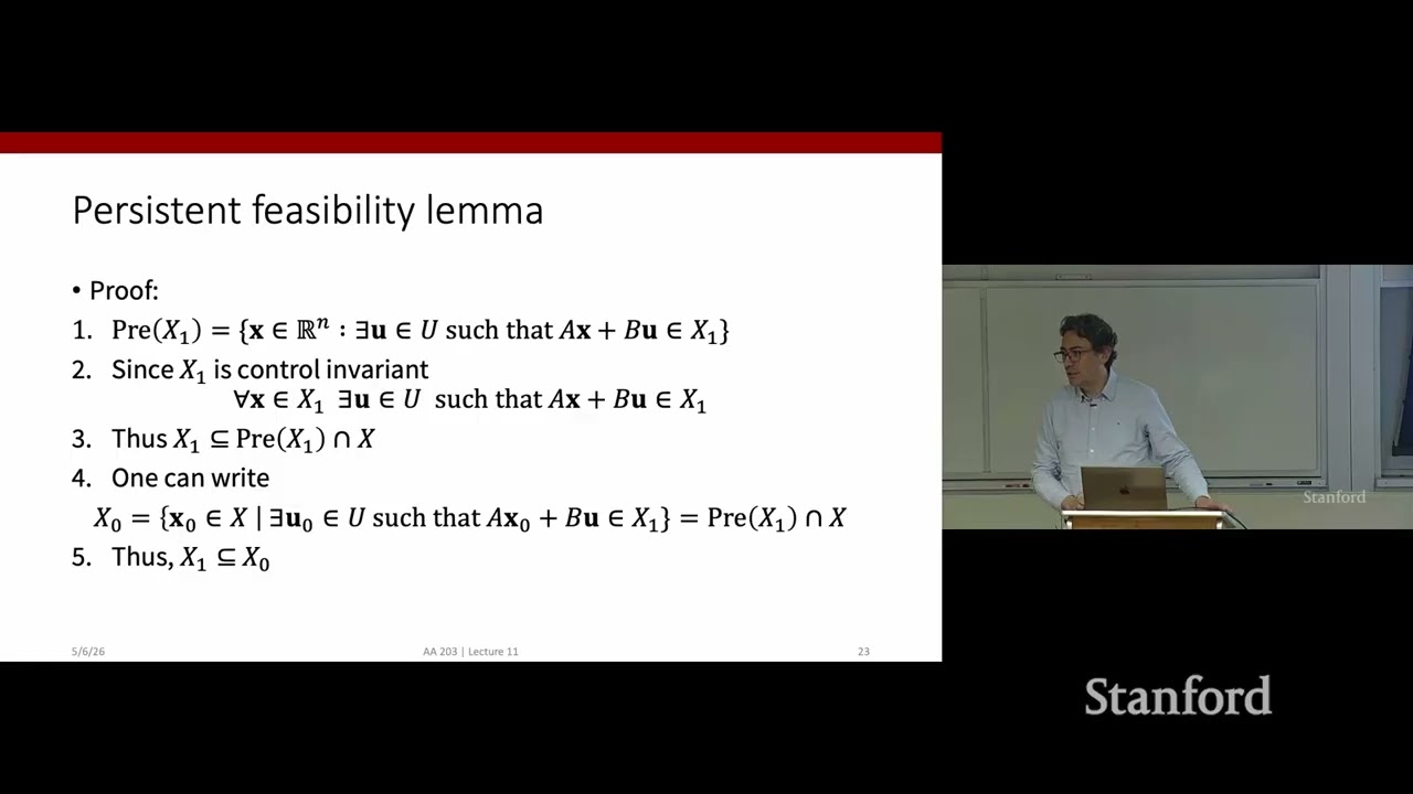
Although jokingly characterized as "not particularly interesting" and "boring," the proof provides a rigorous stress-test of geometric control definitions. To show that the system remains persistently feasible once transitioning to state $x_1$, one must verify that $x_1$ belongs to the set of initial states with feasible horizons, $\mathcal{X}_0$.
```mermaid
flowchart TD
accTitle: Feasibility Set Inclusion Logic
accDescr: Diagram demonstrating how control invariance of X1 implies X1 is a subset of X0 and ensures persistent feasibility.
subgraph Defs["Set Invariance & Reachability"]
A["x in X1"] --> B["Ax + Bu in X1 for some u in U"]
B --> C["x in Pre(X1)"]
end
subgraph Inclusion["Set Inclusions"]
C --> D["X1 subset of (X intersect Pre(X1))"]
D --> E["X0 = X intersect Pre(X1)"]
E --> F["X1 subset of X0"]
end
subgraph Conclusion["Recursive Feasibility"]
F --> G["MPC selects u*(0) in U"]
G --> H["x1 = Ax0 + Bu*(0) in X1"]
H --> I["x1 in X0 (Feasible at next step)"]
end
```
The proof proceeds through the following step-by-step argument:
1. **Definition of One-Step Controllable Set:** The set $\mathrm{Pre}(\mathcal{X}_1)$ is defined as $\{x \in \mathbb{R}^n \mid \exists u \in \mathcal{U} \text{ s.t. } Ax + Bu \in \mathcal{X}_1\}$.
2. **Implication of Control Invariance:** If $\mathcal{X}_1$ is control invariant, then for every $x \in \mathcal{X}_1$, there exists a valid $u \in \mathcal{U}$ such that $Ax + Bu \in \mathcal{X}_1$. Therefore, any point $x \in \mathcal{X}_1$ is automatically inside $\mathrm{Pre}(\mathcal{X}_1)$.
3. **Intersection with State Constraints:** Because points in $\mathcal{X}_1$ must satisfy state constraints, $\mathcal{X}_1 \subseteq \mathcal{X}$. Combining these yields $\mathcal{X}_1 \subseteq \mathcal{X} \cap \mathrm{Pre}(\mathcal{X}_1)$.
4. **Equivalence to $\mathcal{X}_0$:** By definition, $\mathcal{X}_0$ is the set of all $x \in \mathcal{X}$ from which there exists a control sequence generating feasible state trajectories reaching the terminal condition. Equivalently, $\mathcal{X}_0 = \{x \in \mathcal{X} \mid \exists u \in \mathcal{U} \text{ s.t. } Ax + Bu \in \mathcal{X}_1\} = \mathcal{X} \cap \mathrm{Pre}(\mathcal{X}_1)$.
5. **Set Inclusion:** Comparing the expressions proves that $\mathcal{X}_1 \subseteq \mathcal{X}_0$.
When the system starts at $x_0 \in \mathcal{X}_0$, applying the optimal first control $u^*(0)$ drives the system to $x_1 = Ax_0 + Bu^*(0)$. Since this step is the first segment of an admissible trajectory, $x_1 \in \mathcal{X}_1$. Because $\mathcal{X}_1 \subseteq \mathcal{X}_0$, the state $x_1$ also belongs to $\mathcal{X}_0$. Hence, the subsequent MPC optimization problem formulated at state $x_1$ is guaranteed to possess a feasible solution, establishing recursive feasibility by induction.
Prof. Pavone emphasizes that on the final exam, students will definitely be asked to define concepts like control invariant sets.
---
[11:51](https://www.youtube.com/watch?v=8Elrw30y0tg&t=711s) Theorem on Persistent Feasibility via the Terminal Set $X_f$
If the horizon length is $N = 1$, setting the terminal set $\mathcal{X}_f$ to be control invariant directly guarantees feasibility at every step via the previous lemma. To handle general horizons $N > 1$, the following central theorem is introduced:
> **Theorem:** *If the terminal constraint set $\mathcal{X}_f$ is chosen to be a control invariant set for the system under study, then the resulting MPC law is persistently feasible.*
This theorem bridges the theoretical gap, moving feasibility from an abstract property of $\mathcal{X}_1$ to an explicit design parameter, $\mathcal{X}_f$, chosen by the control engineer.
To provide concrete intuition, Prof. Pavone asks what the simplest, most trivial control invariant set is. He jokes, "In any mathematical equation, if you are in doubt, always say zero. Typically zero is the best guess." In this case, the guess is exact: the origin $\{0\}$ is a valid control invariant set. Assuming $u = 0$ is an admissible input (in other words, "doing nothing is typically allowed"), any linear system $x_{k+1} = Ax_k + Bu_k$ starting at $x = 0$ with $u = 0$ transitions directly back to $0$.
The operational intuition is straightforward: if an $N$-step sequence drives the state to the origin by stage $N$, advancing one step forward leaves an $(N-1)$-step sequence that reaches zero. One can then simply append the null control $u = 0$ as the $N$-th input, keeping the system parked at the origin and yielding a valid, admissible $N$-step plan for the next optimization cycle. While $\{0\}$ is an intuitive singleton example, real-world systems can utilize richer, higher-volume control invariant polyhedral sets for $\mathcal{X}_f$.
[14:17](https://www.youtube.com/watch?v=8Elrw30y0tg&t=857s) Choosing the Terminal Set: The Suboptimality of the Origin
Prof. Pavone opens by contrasting arbitrary terminal sets with the broader class of control invariant sets. While forcing the system to reach the origin in $N$ steps ($\mathcal{X}_f = \{0\}$) immediately guarantees persistent feasibility, he poses a fundamental design question to the class: is forcing the state to the origin always the smartest thing to do? The answer is emphatically no. In practical control engineering, the objective is rarely just to drive states to zero at all costs; controllers must also be "very parsimonious in terms of how much control you spend."
Constraining an $N$-step Model Predictive Control (MPC) problem to hit the origin exactly at step $N$ severely restricts the feasible search space. Out of all candidate control sequences, the optimizer is permitted to evaluate only the narrow subset that forces the state to zero within the finite horizon. Typically, those aggressive trajectories demand immense control effort and actuation energy. Thus, while persistent feasibility is mathematically preserved, the controller operates suboptimally, burning excessive control expenditure. For this reason, the terminal constraint $\mathcal{X}_f$—an artificial constraint introduced purely to ensure feasibility—should be kept as relaxed and large as possible to avoid over-constraining the physical system. Designing $\mathcal{X}_f$ represents an ongoing balance between mathematical rigor and engineering pragmatism.
[16:04](https://www.youtube.com/watch?v=8Elrw30y0tg&t=964s) Proof: Control Invariance of $\mathcal{X}_f$ Implies Persistent Feasibility
To provide rigorous backing for these concepts, Pavone presents the proof that choosing a control invariant terminal set $\mathcal{X}_f$ guarantees persistent feasibility of the MPC policy. The proof proceeds by backward induction across truncated feasibility sets:
1. Show that if the terminal set $\mathcal{X}_f$ is control invariant, then the truncated set $\mathcal{X}_{N-1}$ (the set of states that can be steered into $\mathcal{X}_f$ in one step) is also control invariant.
2. Inductively cascade this property backwards: if $\mathcal{X}_{N-1}$ is control invariant, so is $\mathcal{X}_{N-2}$, continuing all the way down to $\mathcal{X}_1$.
3. Once control invariance is established for the one-step feasible set $\mathcal{X}_1$, invoke the previously proven feasibility lemma to conclude that the closed-loop MPC system is persistently feasible.
Focusing on the first inductive step, Pavone defines $\mathcal{X}_{N-1}$ as the truncated feasible set over a one-step horizon—the set of states $x \in \mathcal{X}$ for which there exists an admissible control input $u \in \mathcal{U}$ such that the successor state $Ax + Bu$ lands in the terminal set $\mathcal{X}_f$. To establish that $\mathcal{X}_{N-1}$ is itself control invariant, one must prove that for every state inside $\mathcal{X}_{N-1}$, there exists a control input that transitions the system to another state within $\mathcal{X}_{N-1}$.
By definition, from any point in $\mathcal{X}_{N-1}$, an admissible control steers the state to $x_N \in \mathcal{X}_f$. The critical question is whether this successor state $x_N$ also belongs to $\mathcal{X}_{N-1}$. Because $\mathcal{X}_f$ is assumed to be control invariant, there inherently exists an input $u$ such that $Ax_N + Bu \in \mathcal{X}_f$. But satisfying that exact condition is precisely what qualifies a point for membership in $\mathcal{X}_{N-1}$. Pavone cautions students not to get confused by the subscript indexing: $\mathcal{X}_{N-1}$ denotes a set definition rather than a specific time index, so showing $x_N \in \mathcal{X}_{N-1}$ confirms that one can remain within the set. Repeating this reasoning backward to $\mathcal{X}_1$ and invoking the feasibility lemma completes the proof: an invariant terminal set guarantees persistent feasibility for all future time steps.
```mermaid
flowchart TD
accTitle: Persistent Feasibility Inductive Proof Architecture
accDescr: Flowchart illustrating how terminal set control invariance cascades backward through truncated sets to guarantee persistent feasibility.
subgraph Terminal ["Terminal Condition"]
A["Terminal Set X_f is Control Invariant"]
end
subgraph BackwardInduction ["Backward Invariance Induction"]
B["Truncated Set X_{N-1} is Control Invariant"]
C["Truncated Set X_{N-2} is Control Invariant"]
D["Base Set X_1 is Control Invariant"]
end
subgraph Conclusion ["Feasibility Guarantee"]
E["Invoke Feasibility Lemma"]
F["MPC is Persistently Feasible"]
end
A -->|"1-step reachability"| B
B -->|"induction step"| C
C -->|"cascade to horizon 1"| D
D --> E
E --> F
```
[21:05](https://www.youtube.com/watch?v=8Elrw30y0tg&t=1265s) Design Knobs and Practical Implementation: Tools and Childcare Diseases
Pavone underscores the core takeaway: choosing $\mathcal{X}_f$ to be control invariant with respect to the system dynamics is "a big deal" because it solves the feasibility dilemma. While setting $\mathcal{X}_f = \{0\}$ is always an available option, its practical suboptimality motivates computing richer, larger invariant sets. He notes that dedicated computational toolboxes exist for synthesizing maximal control invariant sets, and students will gain hands-on experience using these algorithmic tools in Problem Set 3.
Midway through this explanation, Pavone is interrupted by a persistent cough, prompting a humorous, weary confession about family life:
- He blames his illness on preschool germs: "I mean, this is my son that brings back bugs from childcare. The child is a biological weapon."
- Realizing the session is being recorded for Stanford Online, he laughs: "I mean, I'm recording. So I'll stop here... just complaining about the diseases that go around in the childcare."
Returning to the technical narrative, he reiterates that $\mathcal{X}_f$ is merely one of three key tuning knobs in the MPC framework. The other two knobs are the terminal cost matrix $P$ and the horizon length $N$. With persistent feasibility resolved via the choice of $\mathcal{X}_f$, the central challenge shifts to tuning $P$ and $N$ to guarantee closed-loop stability.
[22:29](https://www.youtube.com/watch?v=8Elrw30y0tg&t=1349s) Introduction to Stability and the Lyapunov Direct Method
Pavone pivots to the theory of stability, explaining that the primary analytical machinery used in modern MPC is Lyapunov stability. He provides an intuitive, geometric introduction before diving into the formal theorem, considering both discrete-time dynamics $x_{k+1} = f(x_k)$ and continuous-time formulations $\dot{x} = f(x)$.
At an intuitive level, stability asks: if a system starts near an equilibrium point, will its state trajectories remain bounded and return to that equilibrium without going "out of whack"? Pavone illustrates this with the classic mechanical analogy of a ball placed inside a bowl:
- A ball at the bottom of a bowl represents a stable equilibrium. Displacing the ball causes it to oscillate, but natural friction dissipates energy, eventually returning the ball to the bottom.
- Pavone pokes fun at his own accent during the blackboard sketch: "because if you have a ball in a bowl—I never got the pronunciation right. But anyway, so this is a ball and this is a bowl."
- By contrast, balancing a ball on top of an inverted bowl forms an unstable equilibrium; the slightest nudge causes it to roll away indefinitely.
Analyzing stability by solving nonlinear differential or difference equations directly across all initial conditions is practically intractable. Historically, this created a major roadblock in dynamical systems theory until Aleksandr Lyapunov introduced the direct method. Rather than solving for state trajectories explicitly, Lyapunov proposed constructing an energy-like scalar function that decreases monotonically along the system's trajectories. If the system continuously dissipates this generalized "energy," the state is constrained to converge to the point of minimum energy—the equilibrium.
[25:04](https://www.youtube.com/watch?v=8Elrw30y0tg&t=1504s) Lyapunov Stability Theorem and Energy Dissipation Intuition
Building on this physical intuition, Pavone introduces the formal discrete-time Lyapunov stability theorem for an autonomous dynamical system $x_{k+1} = f(x_k)$ with an equilibrium at the origin, meaning $f(0) = 0$.
The formal setup relies on several fundamental components:
- An equilibrium state situated at the origin, satisfying $f(0) = 0$.
- A closed, bounded (compact) set $\Omega$ containing the origin that is positively invariant under the closed-loop dynamics (meaning any trajectory initialized in $\Omega$ remains in $\Omega$ for all forward time).
- A candidate Lyapunov function $V(x)$ (referred to colloquially on the board as $D$ or $V$) defined over $\Omega$.
The Lyapunov function must fulfill three core mathematical properties:
1. **Zero at the origin:** $V(0) = 0$.
2. **Positive definiteness:** $V(x) > 0$ for all non-zero states $x \in \Omega \setminus \{0\}$.
3. **Strict decrease along trajectories:** For all system trajectories evolving within $\Omega$, the value of the function strictly decays at each subsequent time step, such that $V(f(x)) < V(x)$ for all $x \neq 0$.
When these conditions are met, the origin $x = 0$ is proven to be asymptotically stable, guaranteeing that all states starting within $\Omega$ inevitably converge to zero as time tends to infinity. This foundational result establishes the exact framework Pavone will use to design the MPC terminal cost $P$ as a Lyapunov function for the closed-loop optimization.
[27:51](https://www.youtube.com/watch?v=8Elrw30y0tg&t=1671s) Geometric Intuition and Power of Lyapunov Stability
Visualizing a two-dimensional state space clarifies the core geometric intuition behind Lyapunov functions. If an auxiliary scalar function $V(x)$ decreases along all possible system trajectories, the state trajectory is driven down toward the bottom of the bowl—the equilibrium point—because $V(0) = 0$. Physically, this mirrors the intuition that a dynamical system is continuously dissipating energy along its path. The paramount advantage of Lyapunov's direct method is that it establishes stability without requiring explicit integration of differential equations in continuous time or solving closed-form state transition equations in discrete time. As long as one can construct a valid function exhibiting this non-increasing property along trajectories, stability is guaranteed.
```mermaid
flowchart TD
accTitle: Lyapunov Stability Mechanism
accDescr: Concept showing how a candidate Lyapunov function guarantees asymptotic convergence without explicit integration.
subgraph Candidate ["Candidate Function"]
V["Lyapunov Function V(x)<br/>• V(0) = 0<br/>• V(x) > 0 for x ≠ 0"]
end
subgraph Trajectory ["System Evolution"]
Decr["Dissipation Condition:<br/>V decreases along trajectories"]
end
subgraph Outcome ["Stability Conclusion"]
Equil["State Converges to Origin<br/>(Asymptotic Stability)"]
end
V --> Trajectory
Trajectory --> Decr
Decr --> Outcome
```
Constructing such a Lyapunov function is historically the hardest step. In classical physical systems, energy-based arguments often yield natural Lyapunov functions, but other dynamical systems require alternative constructions. Asking the lecture hall how many students have previously encountered Lyapunov stability draws only a few confident hands and an exasperated sigh ("Uf! OK. Well, in that case, read about it"). While the class applies the Lyapunov theorem in a somewhat mechanical way to verify the closed-loop properties of Model Predictive Control (MPC), exploring the broader mathematical and physical literature is strongly recommended. The central question for MPC becomes immediate: what candidate Lyapunov function can be constructed for the closed-loop system?
[32:02](https://www.youtube.com/watch?v=8Elrw30y0tg&t=1922s) The MPC Stability Theorem and Its Assumptions
The development of MPC mirrors recurring historical patterns in engineering. For roughly twenty years, industry practitioners deployed MPC with immense practical success before any rigorous theoretical guarantees existed; only in the 1990s did researchers establish formal stability theory to enable principled parameter tuning. This dynamic is directly comparable to modern deep learning: practitioners use deep neural networks everywhere despite limited theoretical understanding, while existing learning theory often models simplified settings that do not reflect practical deployment.
To establish stability, consider an LQR-style discrete-time setting with linear dynamics and quadratic costs:
- Stage cost: $c(x, u) = x^T Q x + u^T R u$
- Positive definiteness: State weighting matrix $Q \succ 0$, input weighting matrix $R \succ 0$, and terminal penalty matrix $P \succ 0$ (yielding terminal cost $p(x) = x^T P x$)
- Constraint sets: State set $\mathcal{X}$, control set $\mathcal{U}$, and terminal set $\mathcal{X}_f$ are closed and contain the origin
- Control invariance: Terminal set $\mathcal{X}_f$ is control invariant, which directly ensures persistent feasibility of the MPC optimization problem
The fourth condition appears intimidating at first glance: for all $x \in \mathcal{X}_f$, there must exist an input $u \in \mathcal{U}$ such that $A x + B u \in \mathcal{X}_f$ and:
$$c(x, u) + p(A x + B u) - p(x) \le 0$$
Rewriting this inequality as $p(A x + B u) - p(x) \le -c(x, u)$ highlights its Lyapunov-like flavor: because $c(x, u)$ is strictly positive away from the origin, the terminal cost must decrease by at least the stage cost incurred at each step. Reflecting on his own student days, the instructor jokes that encountering this condition felt "like some nightmare of a mathematician." When all four assumptions are satisfied, the closed-loop origin is asymptotically stable, with the set of feasible initial states $\mathcal{X}_0$ serving as the domain of attraction. Beyond proving stability, this theorem provides a practical recipe for selecting MPC design knobs such as the terminal set $\mathcal{X}_f$ and terminal weight matrix $P$.
[36:25](https://www.youtube.com/watch?v=8Elrw30y0tg&t=2185s) Proving Stability: The Optimal Cost as a Lyapunov Function
The proof that follows avoids the tediousness of persistent feasibility proofs, standing out as a particularly elegant and satisfying argument. The core insight is to propose the optimal cost-to-go of the MPC optimization problem initialized at state $x$, denoted $J_0^*(x)$, as the candidate Lyapunov function for the closed-loop system:
$$x_{t+1} = f_{\text{cl}}(x_t) = f(x_t, \mu_{\text{MPC}}(x_t))$$
Once the control input $u$ is replaced by the state-feedback law $\mu_{\text{MPC}}(x)$ obtained by solving the online optimization, the closed-loop dynamics become a pure function of $x$.
To apply Lyapunov's theorem rigorously, several conditions must be checked:
1. **Origin is an equilibrium point:** If initialized at $x = 0$, applying $u_k = 0$ for all horizon steps is feasible because constraint sets contain the origin. With $Q \succ 0$ and $R \succ 0$, the quadratic cost is non-negative and is identically zero for $u = 0$. Since zero is the absolute lower bound of the cost, the all-zero sequence is optimal. Applying $u = 0$ to $x_{t+1} = A(0) + B(0)$ keeps the state at the origin, confirming it is an equilibrium point.
2. **Value at the origin vanishes:** The minimal cost at the origin is strictly zero, confirming $J_0^*(0) = 0$.
3. **Strict positivity away from the origin:** For any state $x \neq 0$, the cost summation over the prediction horizon begins with $k = 0$, which explicitly includes the stage cost term $x_0^T Q x_0$. Because $Q$ is strictly positive definite and $x_0 \neq 0$, this initial term is strictly greater than zero, ensuring $J_0^*(x) > 0$ everywhere outside the origin.
[42:21](https://www.youtube.com/watch?v=8Elrw30y0tg&t=2541s) The Lyapunov Decrease Condition and Shifted Trajectory Bookkeeping
Showing that the optimal cost function $J_N^*(x)$ is strictly positive for non-zero states is the easy half of proving it acts as a valid Lyapunov function. The harder, more fundamental challenge is establishing that this cost strictly decreases over time along the actual trajectories generated by the closed-loop system. Intuitively, this condition ensures the system is continuously dissipating cost or energy, inevitably driving the state down toward its lower bound at the origin. To analyze this, consider any initial state $x_0$ that is feasible for the MPC problem (meaning $x_0 \in \mathcal{X}_N$).
The indexing and bookkeeping can appear clumsy at first glance, but the mechanics are straightforward. At the initial planning cycle (iteration 0), solving the MPC problem yields an optimal control sequence denoted by $(u_0^0, u_1^0, \dots, u_{N-1}^0)$, with an associated predicted state trajectory starting at $x_0^0 = x_0$ and progressing through $(x_1^0, x_2^0, \dots, x_N^0)$. Following the standard MPC policy, only the first control input $u_0^0$ is applied to the plant, causing the system to transition according to its dynamics into the true next state $x_1 = A x_0 + B u_0^0$, which exactly matches the predicted state $x_1^0$.
```mermaid
flowchart TD
accTitle: MPC Shifted Sequence Construction
accDescr: Diagram illustrating the comparison between the iteration 0 optimal sequence and the iteration 1 candidate sequence.
Once at state $x_1$, a candidate control sequence is constructed for stage 1 by taking the tail of the previous optimal sequence, $(u_1^0, \dots, u_{N-1}^0)$, and appending a feasible terminal input $v$. When this shifted sequence is applied starting from $x_1$, the resulting state trajectory replicates the trajectory predicted during the previous cycle from step 2 onward, ending at the new terminal state $A x_N^0 + B v$. A student asks whether the convexity of the quadratic cost alone is enough to guarantee decrease, but Professor Pavone clarifies that one must prove the cost decreases along the specific trajectories produced by the closed-loop feedback law—a property that is not guaranteed a priori. Another student asks if the appended input $v$ is actually executed; Pavone explains that this shifted sequence is simply a "dumb candidate sequence" used as an analytical tool to establish an upper bound on the true optimal cost at $x_1$.
[48:01](https://www.youtube.com/watch?v=8Elrw30y0tg&t=2881s) Constructing a Feasible Candidate Sequence via Control Invariance
To turn this candidate sequence into a rigorous analytical bound, the terminal input $v$ must be chosen intelligently rather than arbitrarily. From the formulation of the MPC problem at time step 0, the final predicted state satisfies the terminal constraint $x_N^0 \in \mathcal{X}_f$. Because the terminal set $\mathcal{X}_f$ is control invariant, there is guaranteed to exist at least one feasible control $v \in \mathcal{U}$ such that the successor state $A x_N^0 + B v$ remains inside $\mathcal{X}_f$.
Selecting this invariant-preserving $v$ guarantees that the entire candidate sequence $(u_1^0, \dots, u_{N-1}^0, v)$ is feasible for the MPC optimization problem initialized at state $x_1$:
- Every control in the shifted sequence satisfies the input constraints $u \in \mathcal{U}$ by construction.
- The intermediate states $(x_2^0, \dots, x_N^0)$ satisfy the state constraints $\mathcal{X}$ because they were already certified as feasible in the cycle 0 solution.
- The final state $A x_N^0 + B v$ satisfies the terminal set constraint by remaining within $\mathcal{X}_f$.
Because this candidate sequence is feasible for the optimization problem at state $x_1$, its associated cost serves as an upper bound on the true optimal cost $J_N^*(x_1)$. In optimization, the optimal cost cannot exceed the cost of any particular feasible candidate:
Establishing this inequality is the pivotal step toward demonstrating that $J_N^*(x_1) < J_N^*(x_0)$, which completes the descent condition needed for Lyapunov stability.
[50:54](https://www.youtube.com/watch?v=8Elrw30y0tg&t=3054s) Algebraic Grouping and Invoking Assumption 3
With the upper bound established, algebraic manipulation reveals how the candidate cost relates to the optimal cost of the previous cycle. By adding and subtracting the terminal penalty $p(x_N^0)$ and the initial stage cost $c(x_0, u_0^0)$, the expression can be rewritten as:
When Pavone asks the class what the first bracketed summation represents, a student identifies it as the optimal cost of the problem initialized at $x_0$, prompting Pavone's enthusiastic reaction: "Exactly. Plus 1 for your grade." Substituting $J_N^*(x_0)$ leaves only the initial stage cost and the terminal bracketed difference.
At this point, Assumption 3 (the Lyapunov descent condition in the terminal set) is brought into play. Assumption 3 states that for all states $x \in \mathcal{X}_f$, there exists an admissible input $u \in \mathcal{U}$ such that $A x + B u \in \mathcal{X}_f$ and:
$$\min_{u \in \mathcal{U}: A x + B u \in \mathcal{X}_f} \left[ p(A x + B u) - p(x) + c(x, u) \right] \le 0$$
By selecting $v$ to be precisely the minimizer $\bar{v}$ that satisfies this condition at $x = x_N^0$, the entire final bracketed term becomes non-positive ($\le 0$). This yields the fundamental descent relation:
$$J_N^*(x_1) \le J_N^*(x_0) - c(x_0, u_0^0)$$
Because the stage cost $c(x_0, u_0^0)$ is strictly positive for any state $x_0 \neq 0$ (owing to the positive definiteness of the quadratic running cost), the optimal cost strictly decreases along the closed-loop trajectory: $J_N^*(x_1) < J_N^*(x_0)$. By standard Lyapunov stability theory, this guarantees that the origin is an asymptotically stable equilibrium for the closed-loop system, with the domain of attraction being the entire set of feasible initial states $\mathcal{X}_N$. Pavone emphasizes the elegance and significance of the derivation: "Is it an interesting proof? I think that's an interesting proof. It's actually quite powerful. So try to go through it a few times just to internalize it."
[57:36](https://www.youtube.com/watch?v=8Elrw30y0tg&t=3456s) Making the Theory Actionable: Stable Open-Loop Dynamics
With theoretical guarantees for persistent feasibility and asymptotic stability in place, the discussion pivots to making these theorems actionable: how does a practitioner explicitly choose the terminal set $\mathcal{X}_f$ and the terminal cost matrix $P$ (where $p(x) = x^T P x$)?
To address synthesis, Pavone introduces the simplest design setting: linear dynamics where the unforced system matrix $A$ is already open-loop asymptotically stable, meaning all eigenvalues of $A$ have magnitude strictly less than 1 (they lie strictly within the unit circle). In this setting, the terminal ingredients can be chosen as follows:
- Define the terminal set $\mathcal{X}_f$ as the maximal positively invariant set for the unforced autonomous system $x_{t+1} = A x_t$ subject to the state constraints $x \in \mathcal{X}$.
- Because the system is unforced ($u = 0$), and $u = 0$ is assumed to be an admissible control ($0 \in \mathcal{U}$), setting $u = 0$ at any state within this set keeps the successor state inside $\mathcal{X}_f$ because $A x + B(0) = A x \in \mathcal{X}_f$. Hence, control invariance is automatically satisfied.
- Numerically, this maximal positively invariant set can be computed directly using standard computational geometry software, such as the Multi-Parametric Toolbox (MPT) in MATLAB, requiring only a few commands to produce the exact polyhedral set representation.
With persistent feasibility secured via this choice of $\mathcal{X}_f$, the remaining question is how to select the terminal cost matrix $P$ so that the Lyapunov descent condition of Assumption 3 holds throughout $\mathcal{X}_f$.
[59:22](https://www.youtube.com/watch?v=8Elrw30y0tg&t=3562s) Tuning the Terminal Cost for Stable Systems via the Lyapunov Equation
The discussion returns to the fundamental requirement imposed by the Lyapunov stability theorem for Model Predictive Control (MPC). Writing the descent condition explicitly for a standard quadratic stage cost and terminal cost, the objective is to ensure that the change in the value function plus the stage cost remains non-positive:
$$-x^T P x + x^T Q x + u^T R u + (Ax + Bu)^T P (Ax + Bu) \le 0 \quad \forall x \in \mathcal{X}_f$$
To verify whether this condition holds, one can test the trivial feedback control law $u = 0$. Setting $u = 0$ causes the control penalty $u^T R u$ and the input terms $Bu$ inside the dynamics to vanish completely. The remaining inequality reduces to:
$$-x^T P x + x^T Q x + x^T A^T P A x \le 0$$
```mermaid
flowchart TD
accTitle: Terminal Cost Selection via Lyapunov Equation
accDescr: Flowchart illustrating how setting u=0 reduces the MPC stability condition to the discrete Lyapunov equation when A is stable.
subgraph StabilityCheck["Stability Condition Check"]
A["Set u = 0 for all x in terminal set X_f"] --> B["Quadratic terms in u drop out"]
B --> C["Resulting relation: A^T P A - P + Q <= 0"]
end
subgraph LyapunovSolve["Matrix Solution"]
C --> D["Recognize discrete Lyapunov equation: A^T P A - P + Q = 0"]
D --> E["If A is asymptotically stable & Q > 0, unique P > 0 exists"]
E --> F["Guarantees persistent feasibility & asymptotic stability"]
end
```
This expression is not merely an arbitrary matrix inequality; it is the celebrated discrete-time Lyapunov equation. If the stage cost weight $Q$ is positive definite ($Q \succ 0$) and the system matrix $A$ is asymptotically stable, there exists a unique positive definite matrix $P \succ 0$ satisfying:
$$A^T P A - P + Q = 0$$
Choosing the terminal cost matrix $P$ as the exact solution to this Lyapunov equation guarantees that the stability condition is satisfied with equality. Consequently, MPC initialized with this choice of $P$ is guaranteed to be asymptotically stable.
The conceptual intuition is straightforward: the MPC horizon is optimized such that after $N$ steps, the system lands inside the maximal positive invariant set $\mathcal{O}_\infty$. If no further replanning were to occur, the natural, unforced stable dynamics would naturally drive the system straight to the origin. In practice, the controller replans at every sampling step and selects different, newly optimized inputs, but the invariant terminal set serves as an indispensable "anchor" ensuring desirable closed-loop behavior. Operationally, this requires only standard computational tools to compute the maximal positive invariant set and a single-line command in MATLAB to solve the Lyapunov equation.
[01:02:56](https://www.youtube.com/watch?v=8Elrw30y0tg&t=3776s) Extending the Design to Unstable Systems via the Riccati Equation
When the autonomous system matrix $A$ is not open-loop stable, the natural dynamics cannot guide the state to the origin without active intervention. In this case, active feedback control must be embedded directly into the terminal design. Instead of assuming $u = 0$, one leverages the infinite-horizon Linear Quadratic Regulator (LQR).
Let $F_\infty$ denote the optimal state feedback gain for the unconstrained discrete-time infinite-horizon LQR problem:
$$u = F_\infty x$$
The terminal set $\mathcal{X}_f$ is then constructed as the maximal positive invariant set for the closed-loop dynamics $(A + B F_\infty)$. This construction ensures that once the state hits $\mathcal{X}_f$ after $N$ steps, even if replanning ceases, the linear LQR control policy remains constraint-admissible and keeps trajectories confined within $\mathcal{X}_f$.
Substituting $u = F_\infty x$ into the stability inequality yields an algebraic expression that is identically satisfied with equality when $P$ is selected as the unique positive definite solution to the Discrete Algebraic Riccati Equation (DARE):
$$P = Q + F_\infty^T R F_\infty + (A + B F_\infty)^T P (A + B F_\infty)$$
This recipe provides a fully procedural, multi-step tuning procedure:
- **If $A$ is stable:** Set $\mathcal{X}_f$ as the maximal positive invariant set under zero input ($u = 0$), and choose $P$ as the solution to the Lyapunov equation.
- **If $A$ is unstable:** Set $\mathcal{X}_f$ as the maximal positive invariant set under the closed-loop LQR controller ($u = F_\infty x$), and choose $P$ as the solution to the discrete-time Riccati equation.
By carving out a region $\mathcal{X}_f$ where the unconstrained linear-quadratic controller is guaranteed to be input- and state-feasible, the LQR cost-to-go acts as an exact Lyapunov terminal penalty.
[01:06:22](https://www.youtube.com/watch?v=8Elrw30y0tg&t=3982s) Explicit MPC and Piecewise Affine Control Laws
While MPC is typically formulated as an online optimization process—measuring the state, solving a quadratic program (QP) in real time on embedded hardware, applying the first control move, and repeating—there exists an offline, explicit counterpart. For linear dynamics subject to polyhedral state and input constraints with quadratic costs, the solution can be precomputed.
The constrained finite-horizon optimal control problem possesses an explicit solution that is continuous and piecewise affine (PWA) over a polyhedral partition of the state space. The state space is partitioned into a finite collection of polyhedral cells $\mathcal{R}_j$:
$$u^*(x) = F_j x + g_j \quad \text{for } x \in \mathcal{R}_j$$
```mermaid
flowchart LR
accTitle: Explicit MPC Lookup Architecture
accDescr: Pipeline of explicit MPC where the state is measured, matched to a polyhedral region, and evaluated via affine gains.
subgraph OnlineExecution["Online Evaluation"]
S["Measure State x"] --> Poly["Point Location in Polyhedral Partition"]
Poly --> Reg["Identify Region R_j"]
Reg --> Law["Evaluate u*(x) = F_j x + g_j"]
end
subgraph OfflinePrep["Precomputed Offline"]
ParamQP["Parametric QP Solver / MPT3"] -.-> Poly
ParamQP -.-> Law
end
```
Under explicit MPC, real-time control requires no numerical optimization solver running on the embedded hardware. The processor simply measures the current state $x$, executes a point-location search in a lookup table to determine which polyhedral cell contains $x$, retrieves the regional gains $(F_j, g_j)$, and evaluates the affine control law directly.
The explicit formulation presents distinct engineering trade-offs:
- **Advantages:** Eliminates the need to embed and certify real-time numerical optimization code. In safety-critical aerospace domains (such as landing a rocket), validating explicit affine lookups is dramatically simpler than guaranteeing that an online solver will converge deterministically without software bugs.
- **Disadvantages:** The polyhedral partition often fragments into a combinatorial explosion of intricately shaped cells as the state dimension or horizon grows. Because modern convex optimization algorithms have advanced substantially, solving a convex QP directly online is often significantly faster than performing spatial point-location queries across a massive lookup table.
Toolboxes such as MPT3 (Multi-Parametric Toolbox 3) automate both the calculation of controlled invariant sets and the multi-parametric quadratic programming required to synthesize explicit controllers.
[01:11:08](https://www.youtube.com/watch?v=8Elrw30y0tg&t=4268s) Transitioning from Regulation to Trajectory Tracking
The focus turns to transitioning MPC from a regulation framework—where the objective is driving the state to the origin—to trajectory tracking. In tracking problems, the control system is provided with a time-varying nominal reference trajectory $x_{\text{ref}}(t)$, often synthesized offline via a direct optimal control method. The MPC layer acts as a feedback wrapper designed to reject disturbances and keep the true trajectory close to the reference.
A naive initial attempt at formulating tracking is to write the stage cost as:
This formulation fails in practical applications. Tracking a dynamic reference trajectory or maintaining a non-zero trim condition inherently requires sustained, non-zero control effort. For example, an aircraft attempting to maintain a constant altitude cannot simply cut off its engines; it requires a persistent, non-zero thrust to counter aerodynamic drag and gravity. Penalizing control effort purely relative to zero ($u^T R u$) introduces an artificial conflict between minimizing state tracking error and penalizing the non-zero control input required to stay on the reference path.
[01:12:21](https://www.youtube.com/watch?v=8Elrw30y0tg&t=4341s) The Oscillation Problem and Delta-Control Formulations
When setting up a standard MPC formulation for tracking using absolute controls, an undesirable pathology often emerges. The moment tracking error drives down to zero, the remaining objective cost becomes completely dominated by the control effort penalty. Consequently, the MPC solver shifts focus to minimizing that input effort, leading it to throttle back—for instance, reducing engine thrust. As soon as thrust decreases, tracking error shoots back up, causing the solver to crank control back up again. This creates a persistent cycle of oscillations bouncing between control effort penalties and tracking error costs.
```mermaid
flowchart TD
accTitle: Tracking Oscillation Cycle in Standard MPC
accDescr: Cycle illustrating how minimizing control effort directly conflicts with zero tracking error in naive MPC formulations.
subgraph Trap["The Naive Penalty Trap"]
A["Tracking error reaches zero"] --> B["Control effort dominates cost"]
B --> C["MPC cuts input effort (e.g., thrust)"]
C --> D["Tracking error spikes back up"]
D --> A
end
```
To resolve this issue, the tracking problem is restructured around "delta controls"—penalizing how inputs vary from one discrete step to the next rather than penalizing their absolute magnitudes. Tracking error is represented by penalizing the deviation of the output $y_k = C x_k$ (where $C$ can simply be identity, yielding $x_k - r_k$ relative to reference $r_k$), accompanied by an input penalty placed purely on rate-of-change variables $\Delta u_k = u_k - u_{k-1}$. Under this reframed objective, achieving steady-state tracking allows for zero tracking error alongside a nonzero, constant physical control (such as steady trim thrust). Because a constant input yields $\Delta u = 0$, both penalty components simultaneously drop to zero, completely harmonizing what the optimizer seeks to minimize with the physical conditions required for stable tracking.
- Absolute controls penalize $u_k$ directly, punishing steady-state trim inputs like hover thrust.
- The delta-control variable is strictly defined as $\Delta u_k = u_k - u_{k-1}$.
- In delta-input tracking formulations, the decision variables solved by the optimizer are the $\Delta u$ increments.
- Starting from a known previous input $u_{t-1}$, actual applied inputs $u_k$ over the horizon are reconstituted recursively by accumulating the solved $\Delta u_k$ steps.
[01:14:28](https://www.youtube.com/watch?v=8Elrw30y0tg&t=4468s) Wrapping Up Known Models and Looking Ahead to Adaptive Control
This discussion brings the foundational first unit of the course to a close. Up to this milestone, every theoretical derivation and algorithmic design assumed a fully characterized system where "everything about the model is known." Starting the following week, the curriculum shifts into unfamiliar territory where system dynamics are partially or entirely unknown. Operating under that uncertainty requires systems to actively adapt on the fly to unmodeled dynamics or learn the missing mechanics in real time while maintaining optimal or near-optimal performance.
The upcoming problem set, P3, will ground these advanced control concepts into practice. Students will explore these MPC architectures firsthand and gain practical experience using the MPT3 (Multi-Parametric Toolbox 3) framework, which provides specialized tools for working with explicit MPC and parametric programming problems.
## Notable quotes
> [00:05](https://www.youtube.com/watch?v=8Elrw30y0tg&t=5s) sometimes people in industry get it wrong — Prof. Marco Pavone
> [01:37](https://www.youtube.com/watch?v=8Elrw30y0tg&t=97s) before the entire setup explodes — Prof. Marco Pavone
> [11:51](https://www.youtube.com/watch?v=8Elrw30y0tg&t=711s) In any mathematical equation, if you are in doubt, always say zero. Typically zero is the best guess. — Prof. Marco Pavone
> [14:17](https://www.youtube.com/watch?v=8Elrw30y0tg&t=857s) very parsimonious in terms of how much control you spend — Prof. Marco Pavone
> [21:05](https://www.youtube.com/watch?v=8Elrw30y0tg&t=1265s) a big deal — Prof. Marco Pavone
> [21:05](https://www.youtube.com/watch?v=8Elrw30y0tg&t=1265s) I mean, this is my son that brings back bugs from childcare. The child is a biological weapon. — Prof. Marco Pavone
> [21:05](https://www.youtube.com/watch?v=8Elrw30y0tg&t=1265s) I mean, I'm recording. So I'll stop here... just complaining about the diseases that go around in the childcare. — Prof. Marco Pavone
> [22:29](https://www.youtube.com/watch?v=8Elrw30y0tg&t=1349s) because if you have a ball in a bowl—I never got the pronunciation right. But anyway, so this is a ball and this is a bowl. — Prof. Marco Pavone
> [27:51](https://www.youtube.com/watch?v=8Elrw30y0tg&t=1671s) Uf! OK. Well, in that case, read about it — Prof. Marco Pavone
> [32:02](https://www.youtube.com/watch?v=8Elrw30y0tg&t=1922s) like some nightmare of a mathematician — Prof. Marco Pavone
> [42:21](https://www.youtube.com/watch?v=8Elrw30y0tg&t=2541s) dumb candidate sequence — Prof. Marco Pavone
> [50:54](https://www.youtube.com/watch?v=8Elrw30y0tg&t=3054s) Exactly. Plus 1 for your grade. — Prof. Marco Pavone
> [50:54](https://www.youtube.com/watch?v=8Elrw30y0tg&t=3054s) Is it an interesting proof? I think that's an interesting proof. It's actually quite powerful. So try to go through it a few times just to internalize it. — Prof. Marco Pavone
> [01:14:28](https://www.youtube.com/watch?v=8Elrw30y0tg&t=4468s) everything about the model is known — Prof. Marco Pavone
## Mentioned
Aleksandr Lyapunov, Discrete Algebraic Riccati Equation (DARE), Linear Quadratic Regulator (LQR), MATLAB, Model Predictive Control (MPC), Multi-Parametric Toolbox (MPT / MPT3), Prof. Marco Pavone, Stanford Online
## Video description
Lecture 12 — Persistent Feasibility of MPC, Stability, and Explicit MPC
Read the companion textbook, Principles of Robot Autonomy, free online: https://porabook.com
To learn more about enrolling in AA203 Optimal and Learning-Based Control, visit: https://online.stanford.edu/courses/aa203-optimal-and-learning-based-control
Follow along with the course schedule and syllabus: https://stanfordasl.github.io/aa203/sp2526/
Bio: Dr. Marco Pavone is an Associate Professor of Aeronautics and Astronautics at Stanford University and a Senior Director of Autonomous Vehicle Research at NVIDIA. Prior to joining Stanford, he was a Research Technologist in the Robotics Section at NASA’s Jet Propulsion Laboratory. Dr. Pavone received his Ph.D. in Aeronautics and Astronautics from the Massachusetts Institute of Technology in 2010. His research focuses on the analysis, design, and control of autonomous systems, with particular emphasis on self-driving cars, autonomous aerospace vehicles, and future mobility systems. He has been recognized with numerous awards, including the Presidential Early Career Award for Scientists and Engineers from President Barack Obama, the Office of Naval Research Young Investigator Award, the NSF CAREER Award, the NASA Early Career Faculty Award, the IEEE Kiyo Tomiyasu Award, the CSS Award for Technical Excellence in Aerospace Control, and the Early-Career Spotlight Award from the Robotics Science and Systems Foundation.
Instructors:
Prof. Marco Pavone, Associate Professor of Aeronautics and Astronautics, Director of Autonomous Vehicle Research at NVIDIA
Dr. Daniele Gammelli, Research Director at the Italian Institute of Artificial Intelligence (AI4I), Researcher at the Department of Aeronautics and Astronautics, Stanford University
Full playlist: https://www.youtube.com/playlist?list=PLa9dmHsLK9dg
Professor Marco Pavone demonstrates how Model Predictive Control (MPC) guarantees persistent feasibility and asymptotic stability by coupling control invariant terminal sets with Lyapunov-based terminal penalties, while detailing practical adaptations for offline computation and trajectory tracking.
Invariant Terminal Sets Guarantee Recursive Feasibility (11:51)
Persistent feasibility requires an MPC optimization solver to produce a valid candidate solution at every future replanning cycle. Pavone outlines the foundational Feasibility Lemma: if the one-step truncated set X_1 is control invariant, then X_1 is a subset of the feasible initial set X_0. Because an optimal first control move steers the system into X_1, this set inclusion guarantees that the next optimization problem formulated at state x_1 remains feasible. For arbitrary horizons N, choosing the terminal constraint set X_f to be control invariant ensures persistent feasibility by inducing invariance backward across all truncated sets down to X_1.
While setting the terminal set to the origin (X_f = {0}) trivially fulfills invariance, Pavone highlights that doing so severely restricts the optimization search space. Forcing the system to reach zero in exactly N steps demands aggressive, energy-intensive control effort, resulting in suboptimal performance. To balance theoretical feasibility with control parsimony, practical engineering formulations keep X_f as large as possible by computing maximal polyhedral invariant sets using specialized toolboxes.
Closed-Loop Stability via Optimal Cost Descent (36:25)
To certify asymptotic stability toward the origin, the closed-loop MPC formulation employs the optimal cost-to-go J_N*(x) as a Lyapunov function. By construction, J_N*(0) = 0, and strictly positive definite stage cost matrices (Q > 0, R > 0) ensure J_N*(x) > 0 for all non-zero states. The key analytical requirement is that within the terminal set X_f, there exists an admissible input such that the terminal penalty decrease satisfies p(Ax + Bu) - p(x) <= -c(x, u), meaning the terminal value decays by at least the stage cost.
Strict decay along closed-loop trajectories is established by analyzing a candidate control sequence formed by taking the tail of the previous cycle's optimal plan and appending an invariant-preserving input v in X_f. Because this candidate trajectory is feasible at state x_1, its cost upper-bounds the true optimal cost J_N*(x_1). Substituting the terminal descent condition yields J_N*(x_1) <= J_N*(x_0) - c(x_0, u_0), confirming that the value function strictly decreases over time and proving asymptotic stability with the feasible initial set X_0 as the domain of attraction.
Tuning Terminal Parameters via Matrix Equations (59:22)
Translating stability conditions into actionable design choices depends on the open-loop stability of the system matrix A. When A is asymptotically stable, X_f is chosen as the maximal positively invariant set under zero input (u = 0). Under this choice, setting u = 0 reduces the terminal descent inequality to the discrete-time Lyapunov equation: A^T P A - P + Q = 0. Solving this equation yields a unique positive definite matrix P that guarantees closed-loop stability.
For open-loop unstable dynamics, zero control cannot steer the system to the origin. Instead, practitioners incorporate an unconstrained infinite-horizon Linear Quadratic Regulator (LQR) feedback law, u = F_inf * x. In this architecture, X_f is defined as the maximal positive invariant set under the closed-loop dynamics (A + B * F_inf), and P is selected as the unique positive definite solution to the Discrete Algebraic Riccati Equation (DARE). This configuration ensures the unconstrained LQR cost-to-go functions as a valid Lyapunov terminal penalty while enforcing constraint satisfaction.
Explicit Lookups and Delta-Control Tracking Formulations (66:22)
Beyond real-time quadratic programming, constrained linear MPC can be evaluated offline as explicit MPC, yielding a continuous, piecewise affine control law defined over a polyhedral partition of the state space. In real-time execution, the controller performs a point-location lookup to retrieve region-specific gains and evaluates an affine equation without running an online solver. While this approach simplifies safety certification in embedded applications like aerospace, Pavone notes that cell partitions suffer from combinatorial growth as dimensions or horizons scale, often making modern online QP solvers faster than large table lookups.
When shifting from origin regulation to trajectory tracking, naively penalizing absolute control effort (u^T R u) creates persistent oscillations because maintaining steady-state trim requires sustained non-zero control. If the tracking error vanishes, the optimizer throttles input to reduce the control penalty, reigniting the tracking error. To prevent this cycle, MPC formulations adopt delta controls by penalizing the input rate of change, delta_u_k = u_k - u_{k-1}. This allows steady-state trim inputs with zero tracking error without incurring cost penalties.
This lecture completes the foundational analysis of MPC for fully known linear models; subsequent lectures shift toward adaptive control and online learning methods designed for systems where the underlying dynamics are partially or entirely unknown.
Source quotes
[0:05] Prof. Marco Pavone: sometimes people in industry get it wrong
[1:37] Prof. Marco Pavone: before the entire setup explodes
[11:51] Prof. Marco Pavone: In any mathematical equation, if you are in doubt, always say zero. Typically zero is the best guess.
[14:17] Prof. Marco Pavone: very parsimonious in terms of how much control you spend
[21:05] Prof. Marco Pavone: a big deal
[21:05] Prof. Marco Pavone: I mean, this is my son that brings back bugs from childcare. The child is a biological weapon.
[21:05] Prof. Marco Pavone: I mean, I'm recording. So I'll stop here... just complaining about the diseases that go around in the childcare.
[22:29] Prof. Marco Pavone: because if you have a ball in a bowl—I never got the pronunciation right. But anyway, so this is a ball and this is a bowl.
[27:51] Prof. Marco Pavone: Uf! OK. Well, in that case, read about it
[32:02] Prof. Marco Pavone: like some nightmare of a mathematician
[42:21] Prof. Marco Pavone: dumb candidate sequence
[50:54] Prof. Marco Pavone: Exactly. Plus 1 for your grade.
[50:54] Prof. Marco Pavone: Is it an interesting proof? I think that's an interesting proof. It's actually quite powerful. So try to go through it a few times just to internalize it.
[74:28] Prof. Marco Pavone: everything about the model is known
Original transcript
[0:05] All right.
[0:06] Let's get started.
[0:07] So today, we're going to
continue our discussion
[0:09] about MPC.
[0:10] In particular.
[0:11] We're going to wrap
up our discussion
[0:12] about persistent feasibility
as one of the key properties
[0:16] we want to imbue in our
MPC control pipeline.
[0:20] And then we'll switch to
the topic of stability.
[0:23] So not only we want to make sure
that MPC loop has a feasible
[0:28] solution at each point
in time, but we also
[0:30] want to make sure
that whatever action
[0:32] we optimize for does
something useful.
[0:35] In our problem
setting, useful means
[0:37] we are stabilizing the system
that is converging to 0.
[0:41] We'll then wrap
up the discussion
[0:43] with a couple of topics that
are of practical relevance,
[0:50] specifically how some
of the optimization
[0:52] could actually be computed
offline as opposed to online.
[0:56] That was actually a pretty big
deal about 10 years ago where
[0:59] hardware was not
particularly advanced yet,
[1:02] and optimization solvers were
not particularly advanced yet.
[1:05] So offloading part of
optimization offline
[1:09] was a big deal
because it relieved
[1:11] what you had to do online.
[1:13] So basically, you
minimize delays.
[1:15] And then we're going to talk
about the application of MPC
[1:18] to a slightly more
general setting, which is
[1:20] that of a trajectory tracking.
[1:22] And I will show you how
the MPC formulation has
[1:25] to be modified a little
bit to ensure that you have
[1:28] a good tracking performance.
[1:30] Interestingly enough, sometimes
people in industry get it wrong.
[1:33] So I want to make sure that you
are not one of those people.
[1:37] All right.
[1:38] So last time, we introduced
the concept of MPC.
[1:42] It's a bit dark here.
[1:46] Let's leave it at this before
the entire setup explodes.
[1:50] So we talked about MPC.
[1:54] I introduced the concept.
[1:55] I introduced a specific
problem set up,
[1:59] which is that of controlling
a linear time varying system.
[2:03] Such were two
polyhedral constraints.
[2:06] We talked about the problem
persistent feasibility
[2:10] and stability.
[2:11] We introduced some concepts,
in particular the concept
[2:14] of a one-step controllable
set, the concept
[2:17] of controlling variance
set, the concept
[2:19] of a positive environment set,
the concept of feasibility set.
[2:23] And then we stated
the lemma, which
[2:25] reads as if set x1,
which is essentially
[2:29] truncated feasibility
set, where we look
[2:31] at feasible state control
pairs starting from stage
[2:38] 1 as opposed to 0.
[2:39] Well, if this set x1 is control
invariant set for the system
[2:44] under consideration,
then the MPC law
[2:47] is persistently
feasible, which means
[2:49] that at each planning
cycle, we have
[2:51] at least one feasible solution.
[2:53] As I mentioned last
time, this result per se
[2:56] is not particularly
useful, because x1 is not
[3:00] one of the tuning knobs that
you can manipulate in order
[3:03] to tune your MPC.
[3:04] But we'll see it's a stepping
stone for the theorem
[3:08] that I'm going to state in a few
minutes that actually relates
[3:12] the concept of
persistent feasibility
[3:14] to one of our tuning knobs.
[3:16] The t is actually
the terminal set, xf,
[3:20] that we use as one of the
constraints in our MPC
[3:23] formulation.
[3:26] With that context, let's
prove this feasibility lemma.
[3:30] The proof is not
particularly interesting,
[3:36] but at least it stress
tests your understanding
[3:39] of some of the concepts
we have discussed so far.
[3:45] So remember that we
want to show that--
[3:50] sorry.
[3:52] If x1 is control invariant
set, then the MPC low
[3:57] is persistently feasible.
[3:58] So once we transition
to the new state
[4:01] from the perspective
of the new state x1,
[4:03] we still have a control that is
feasible over the optimization
[4:06] horizon.
[4:08] So the proof is as follows.
[4:12] Remember the definition of
a one-step controllable set.
[4:18] So the one-step controllable
set to x1 or previous of x1
[4:23] is defined as the set of states.
[4:25] That's just the definition
that we stated last time.
[4:27] It's defined as a set
of states in Rn, such
[4:31] that there exists a
control, a feasible control,
[4:34] such that Ax plus Bu
transitions into the set x1.
[4:40] So that's the definition
of a one-step control set.
[4:46] Now, since x1 is
control invariant,
[4:52] again, by definition
of control invariance
[4:54] for all states within x1, there
exists a feasible control such
[5:00] that Ax plus Bu is in X1.
[5:05] Now, if we compare
the two definitions,
[5:10] we see that x1, a point
that is in x1 also
[5:18] belongs to the previous of x1.
[5:22] So the one-step controllable
set is the same property.
[5:27] But the point that is in x1
also has to be in capital X,
[5:32] by the definition of x1.
[5:36] X1 is first of all the set of
states that are feasible so
[5:40] that are in x, which
means that the set
[5:49] x1 has to be a subset of the
intersection between the set x.
[5:55] This is trivial and
the previous of x1.
[6:01] Does it make sense?
[6:02] It's a bit of a
mouthful, but it just
[6:05] follows from the definitions.
[6:08] Now, let's go back one step and
now reason in terms set X of 0.
[6:16] So this is the set
of states, x of 0,
[6:21] such that there is a
sequence of controls,
[6:24] such that the states
generated under the dynamics
[6:27] are produced states
that are feasible.
[6:33] Remember the definition of X0.
[6:35] X0 is the set of feasible
states such that there exists
[6:40] a sequence of controls,
feasible controls,
[6:43] such that under the
dynamics evolution,
[6:48] the generated states are
also feasible and satisfy
[6:51] the terminal condition.
[6:53] Now, I can rewrite
the definition of X0
[6:56] as the set of
feasible states such
[7:01] that there is a feasible control
such that X1 belongs to capital
[7:06] X1 because capital X1 subsumes.
[7:09] What is the definition of an x1?
[7:11] Previous slide.
[7:13] The fact that there is
a truncated sequence
[7:15] of controls that leads to a
feasible state trajectory.
[7:33] Now, again, let's compare this
definition to the definition
[7:39] here.
[7:40] So they are identical.
[7:42] The only difference
is that in here, I'm
[7:44] imposing these additional
constraints so that the state
[7:47] has to belong to X.
[7:49] So X0 is really the
intersection of capital X
[7:54] and the one-step
controllable set to X1.
[7:58] But then we put
together the two facts,
[8:00] and we see that X1
is subset of X0.
[8:05] Every state that belongs to X1
is also a state belongs to X0.
[8:10] Does this make sense?
[8:11] It's mostly basically
pattern-matching
[8:13] the different definitions.
[8:15] So there is no particular
cleverness here.
[8:17] Yes.
[8:17] So in the previous example, it's
not necessarily a subset of X,
[8:23] because--
[8:24] No, no, because of
how we define it here.
[8:30] It's any state that
transitions us into X1.
[8:34] It could also be a
state that is not
[8:36] feasible in terms set
membership to capital X. OK.
[8:44] So now there is a slightly
more interesting part.
[8:48] Actually, this entire
proof is quite boring.
[8:50] Take some state that belongs
to X of 0, some initial state.
[8:56] And let U star 0 be the solution
to the finite-time optimization
[9:01] problem, MPC
optimization problem.
[9:04] Let U star 0 be in the first
control in this sequence.
[9:09] Then under the
control, you start 0.
[9:11] Under the MPC control, we
transition to a new state X1.
[9:17] Since you U star 0
is clearly feasible,
[9:19] X1 belongs to capital X1 because
it's part of the MPC trajectory.
[9:26] So by definition, it has
to satisfy all the state
[9:28] constraints under the
dynamics evolution.
[9:32] And so it belongs to X1.
[9:34] But we just prove
that set X1 is subset
[9:38] of X0, which means that
set X1 belongs actually
[9:42] to set X of 0, which means
that the new MPC optimization
[9:47] problem is indeed feasible.
[9:49] And then you can recursively
apply this property
[9:51] through time.
[9:54] So rewinding all
of this, we wanted
[9:56] to prove that under the MPC
control law, the new state
[10:01] X of 1, X1 belongs to X0, the
set of feasible states for MPC.
[10:09] To do so, we
manipulated a little bit
[10:12] the definition of a
one-step controllable set
[10:15] and the notion of
control invariance.
[10:19] And we finally proved
that if set X1 is
[10:30] control invariant,
then the problem,
[10:32] the MPC problem is
persistently feasible.
[10:34] Does it make sense?
[10:35] Again, not a particularly
exciting result, not
[10:38] also particularly useful, but
it's a good stress test for you
[10:41] to see whether you
understand the notion
[10:45] of a one-step controllable
set, control invariant set,
[10:47] and so on.
[10:48] In the final exam, there will
be have one question that
[10:50] will-- well, I will ask you what
is say a control invariant set.
[10:55] OK.
[10:57] Anyway-- so say that the
horizon is equal to 1.
[11:09] Then we can just
choose the terminal
[11:13] set to be controlling violence.
[11:14] And by the previous lemma, we
know that if that is the case,
[11:18] then the MPC problem is feasible
at all replanning stages.
[11:26] But of course, in general,
the optimization horizon
[11:29] is greater than 1.
[11:30] So how can we extend
these results to the cases
[11:33] whereby we have a general
optimization horizon capital N?
[11:37] So that's what we're
going to do next.
[11:43] Any questions in the meantime?
[11:51] So now we get to the
more interesting part.
[11:58] So building on the lemma
that I just showed,
[12:00] it says that if X1 is
controlled invariant,
[12:03] then the MPC control law
is persistently feasible.
[12:06] Now, we can prove a
more powerful theorem
[12:09] that reads as follows.
[12:11] If the set X of f,
which is a reminder,
[12:14] is the set through which we
specify a terminal constraint
[12:19] for the MPC
optimization problem,
[12:21] it's something that we decide.
[12:24] And if set X of f is a control
invariant set for the system
[12:29] under study, then the MPC
law is persistently feasible.
[12:35] That's interesting.
[12:37] Let's try to understand
what is this saying.
[12:39] What is a trivial control
invariant set for this system?
[12:44] Meaning a set that
if you are there,
[12:46] there exists a control that
allows you to stay there.
[12:52] By any mathematical equation, if
you are in doubt, always say 0.
[12:56] I mean, typically 0
is the best guess.
[12:59] In this case, it's correct.
[13:00] So the origin 0 is indeed
a control invariant set.
[13:05] If your state is X
equals 0, assuming
[13:09] that U equals 0 is an allowable
control, which is typically
[13:13] true, I mean, doing nothing
is typically allowed.
[13:17] Under linear dynamics, if you
are at 0 and you use Control 0,
[13:22] your next state is 0, which
means that the origin, you
[13:26] have a set with only one
point, but still it is a set.
[13:29] The origin is indeed a
control invariant set.
[13:33] And intuitively,
what does it say?
[13:37] It's saying that if we just
target the origin in N steps
[13:43] and then I shrink
the horizon by 1,
[13:46] there is always an admissible
control sequence that
[13:50] is the concatenation
of the previous control
[13:53] sequence and then the fact
that with the last control
[13:56] we just say at 0.
[13:57] So you can just trivially
continue your control sequence
[14:00] to have a full and
step control sequence.
[14:03] So we're going to
prove the theorem,
[14:06] but the intuition
is quite obvious.
[14:09] That said, for a
general system, you
[14:13] might have different
control invariant set.
[14:15] 0 is just an option.
[14:17] But actually, you could
have a larger set,
[14:19] which is the control
invariant for the system.
[14:21] We'll see later how to
compute those larger sets.
[14:25] So do you think that the origin
is always the best choice?
[14:31] So constraining your system
to reach the origin in N step
[14:34] as part of your MPC
control law, you
[14:37] think that this is always
the smart thing to do?
[14:39] It guarantees you
persistent feasibility.
[14:41] So that's great.
[14:47] Remember that
typically, you're not
[14:50] just reasoning in terms of
controlling the state to 0,
[14:54] but you also want to be
very parsimonious in terms
[14:57] of how much control you spend.
[15:00] So oftentimes,
asking your system
[15:02] to reach the origin in N steps
as part of your MPC optimization
[15:07] problem can be very limiting.
[15:09] So basically, you
are asking-- so
[15:11] of all the control
sequences you could apply,
[15:13] you're only optimizing
over those that
[15:15] in N step new to the origin.
[15:17] It's typically those that
require a lot of control effort.
[15:20] So yes, you have
persistent feasibility,
[15:23] but now, you might control
your system very suboptimally,
[15:27] meaning with a lot of
control expenditure.
[15:30] So that's why in general,
the terminal constraint--
[15:35] it is something that you
artificially add to your MPC
[15:37] problem to ensure
persistent feasibility--
[15:40] should be as relaxed as possible
so that you don't overly
[15:43] constrain your system.
[15:44] Does that make sense?
[15:46] Just trying to give you
both mathematical backing
[15:52] for what I'm saying, but also
some practical considerations.
[15:56] And this is stuff that
people do for real.
[15:58] So it's constantly a little
bit of a design choice
[16:02] how to properly set X of f.
[16:04] So now, let's
prove this theorem.
[16:09] So the proof is as follows.
[16:13] So we prove that if X of f
is control invariant, then
[16:18] XN minus 1, the truncated set,
where your horizon is only 1,
[16:24] is also going to be
control invariant.
[16:27] And then if XN minus 1
is control invariant.
[16:29] XN minus 2 is control invariant.
[16:31] All the way to x1,
and once we hit x1,
[16:34] we know from the
previous lemma that if x1
[16:37] is controlling violent, then the
system is persistently feasible.
[16:39] So we can invoke that
lemma to conclude
[16:42] the proof of the theorem.
[16:45] So let's start with
the first step.
[16:47] So if Xf-- we want to prove
that if Xf is control invariant,
[16:52] XN minus 1 is control
invariant too.
[16:56] XN minus 1 is defined as usual.
[17:00] Now it's just a
truncated feasibility
[17:04] set where we only reason in
terms of a one-step horizon.
[17:07] It's the set of states, feasible
states for which there exists
[17:11] a feasible control such that
under the system dynamics,
[17:16] we have a sequence of
states that is feasible.
[17:19] In this case, the last state
needs to satisfy the terminal
[17:25] constraint.
[17:32] Now, because of the terminal
constraint, we know that--
[17:44] remember that we want to show
that this set is controlled
[17:47] invariant.
[17:48] So the question
is for any state,
[17:52] any vector within
the state, is there
[17:56] a control input that allows us
to transition back into this
[18:00] set under the system dynamics?
[18:04] So that's what we want to prove.
[18:06] Now, what we know is that by
the definition of XN minus 1,
[18:15] there exists a control such
that XN minus 1 plus B1
[18:20] is equal to XN, which belongs
to the terminal set X of f.
[18:24] I mean this is by
essential definition of x1.
[18:29] Now, the question is does
XN which belongs to Xf also
[18:36] belong to X1?
[18:38] If that is true, that means
that X1 is control invariant.
[18:42] I found actually a
control that allows
[18:44] me to transition back into X1.
[18:48] But for now, the only thing
that I know is that X of N
[18:52] belongs to Xf.
[18:55] But from the assumption of the
theorem, we do know that X of f
[19:00] is a control
invariant set, which
[19:04] means that there exists a U
such that Ax plus Bu belongs
[19:11] to X of f.
[19:14] But isn't that the
definition of the--
[19:17] defines the membership
of a point to XN minus 1.
[19:22] So we have just proved
that XN minus-- that XN
[19:26] indeed belongs to
capital set XN minus 1.
[19:29] Don't be mixed up
with the subscript X--
[19:34] XN minus 1 is just a
definition of a set.
[19:37] Is it a one-step feasible set?
[19:40] So the fact that XN
belongs to X minus 1
[19:42] doesn't tell you nothing in
terms of the temporal coherency
[19:45] between the subscripts.
[19:47] So we have just proven that X of
N belongs to capital XN minus 1.
[19:54] So we have just
proved that X minus 1
[19:56] is indeed in control invariant.
[19:58] But then you can apply this
argument recursively until--
[20:03] to prove that X minus 2 is
control invariant, x minus 3
[20:06] is control invariant,
all the way to X1.
[20:08] At that point, we invoke
the feasibility lemma
[20:11] from the previous
lecture, and then
[20:13] we can state the claim, that
if Xf is controlled invariant,
[20:17] then MPC is
specifically feasible.
[20:21] Does this make sense?
[20:23] Again, there's a
little bit of pattern
[20:25] matching with definitions.
[20:28] Most important thing
for you to understand
[20:31] is-- and this is a big deal.
[20:33] If the set Xf is chosen
to be a controlling
[20:39] set for aerodynamics, then set
your MPC is perfectly feasible.
[20:43] Now, the origin is in general
a control invariant set.
[20:49] So it's a possible choice
for your terminal constraint.
[20:52] In general, it's
a bit suboptimal.
[20:54] So we want to have more
sophisticated choices
[20:58] for the terminal set within all
the possible ways of defining
[21:03] a control invariant set.
[21:05] We'll get back.
[21:07] We'll get back to
this point later along
[21:10] with a pointer to a
computational tool that
[21:14] allows you to compute
control invariant sets.
[21:17] And in problem set 3,
you'll have a few problems
[21:21] that will expose you to how
to use this toolbox in order
[21:26] to compute control
invariant sets.
[21:35] I mean, this is my
son that brings back
[21:38] bugs from a childcare.
[21:40] This is-- the child is
a biological weapon.
[21:44] This is my fourth or five--
[21:45] I mean, I'm recording.
[21:46] So I'll stop here.
[21:48] So we're just complaining
about the diseases that
[21:51] go around in the childcare.
[21:53] Anyway, so the
terminal set X of f
[21:56] is introduced artificially for
the sole purpose of leading
[21:59] to a sufficient condition
for persistent feasibility.
[22:02] It's one of the tuning knobs.
[22:04] And now we know that at least
from an abstract standpoint,
[22:07] if we choose X of f to be
controlling variance set,
[22:10] persistent feasibility
is guaranteed.
[22:13] As I said, the
simplest choice would
[22:15] be to just pick X
of f as the origin,
[22:18] but this is
generally undesirable
[22:20] because it excessively restricts
the space of feasible control
[22:25] sequences.
[22:26] We'll discuss this choice
later in more detail.
[22:29] Now we switch to the other topic
which is that of stability.
[22:34] Now we know at least how to
make the problem persistently
[22:36] feasible.
[22:37] The tuning knob that at least
for the scope of this class
[22:40] we choose for that
purpose is the control--
[22:42] the terminal constraints X of f.
[22:45] We have other two tuning knobs,
how we select the terminal cost
[22:50] P in our MPC formulation and
how we select the horizon N.
[22:55] So the question now is,
can we tune those tuning
[22:59] knobs in such a way that
stability is guaranteed?
[23:09] To prove stability,
we will leverage
[23:12] the tool of Lyapunov stability.
[23:14] Some of you may already
be familiar with,
[23:16] but if you are not, no problem.
[23:18] I'll give you a very quick
intro to Lyapunov stability.
[23:24] So what does Lyapunov
stability say?
[23:27] I will state in a
second the full theorem,
[23:31] but first, I want to
give you intuition.
[23:34] So say that you have
a dynamical system.
[23:39] SK plus 1 equal F of XK, or
maybe in continuous time,
[23:46] you also have X
dot equal F of x.
[23:50] Now, the question is
is the system stable?
[23:55] Roughly speaking, if you start
close to an equilibrium point,
[24:00] will you go back to
that equilibrium point
[24:05] without having trajectories
that go out of whack?
[24:12] If this is a ball, this is
a stable equilibrium point,
[24:17] because if you have
a ball in a ball--
[24:21] I never got the
pronunciation right.
[24:23] But anyway, so this is a
ball and this is a ball.
[24:26] And so if you have
a ball in a ball,
[24:31] you know that if you start this
ball outside of the equilibrium
[24:35] point, then it will
start oscillating.
[24:38] And then if you have a
little bit of friction,
[24:40] you dissipate energy.
[24:42] You will go back to
the bottom of the ball.
[24:46] So this is the case of a
stable equilibrium point.
[24:49] If you are here, of
course, this is unstable.
[24:53] This is an equilibrium point.
[24:54] So if you put the ball
here, it will stay here.
[24:56] But then if you start a little
bit farther from equilibrium
[24:59] point, it will go down.
[25:04] So say that you have
a dynamical system
[25:07] and say that you have
equilibrium point
[25:08] and you want to understand
if the dynamics are
[25:11] at least locally stable
around that equilibrium
[25:13] point, how can you show that?
[25:17] Well, all that you know is that
you have an equilibrium point,
[25:22] and you have a
transition dynamics.
[25:24] So in principle, what
you will need to do
[25:25] is to solve for all
possible initial conditions
[25:29] around your equilibrium
point, your discrete time
[25:32] equation, or
differential equation,
[25:35] and then see what happens.
[25:38] Now, in general, solving
nonlinear differential equation
[25:41] or also discrete time nonlinear
update equations is complicated.
[25:47] So for the longest time,
this was a big problem.
[25:51] Then there was a guy,
Lyapunov, that came in
[25:53] and saying, well, maybe
we can say something
[25:55] about the stability
of the system
[25:56] without reasoning
directly in terms
[25:58] of the evolution of the state.
[26:03] The idea is if we can say that
there is some function that,
[26:08] loosely speaking, has a notion
of an energy function, that
[26:12] decreases over time
along the system
[26:16] trajectories, that could tell
me something about the evolution
[26:21] of the underlying system.
[26:23] Think about energy being
dissipating along the evolution
[26:26] of a system.
[26:27] That means that basically
the system inherently
[26:30] is constraint to reach a
point of minimum energy
[26:35] because you are
dissipating energy.
[26:37] So basically, the
institution is if I
[26:39] don't need to prove that all
the trajectory goes to 0.
[26:41] If I can say, tell to the system
that the system is dissipating
[26:44] energy, then probably,
it will converge
[26:46] to some state of minimum
energy, loosely speaking.
[26:51] So that's basically what
the Lyapunov theorem
[26:54] says, considering the
equilibrium point for a system
[26:57] XK plus 1 equal of F of XK.
[27:01] Equilibrium point means
that if you are at 0, F of 0
[27:05] is equal to 0, meaning
that we stay there.
[27:09] Let's consider a set omega,
which is closed-bounded
[27:12] and positively invariant set.
[27:14] This is some mathematical
thing that we
[27:16] need, not super important.
[27:19] Let D refer to it as
the Lyapunov function,
[27:23] be a function that has
the following property.
[27:26] It's a Z origin.
[27:28] It's a positive
outside of the origin.
[27:31] And for the evolution
of system trajectories
[27:36] starting from omega,
then this function
[27:40] decreases along
the trajectories.
[27:45] Then X equals 0 is
asymptotically stable.
[27:51] So essentially, you have--
[28:03] this is your V
function, V of X. This
[28:08] is a two-dimensional
state space.
[28:12] If I can say that along all
possible system trajectories
[28:19] V decreases in value, it means
that the state trajectory
[28:25] is going to the bottom, which is
the equilibrium point, since V0
[28:30] is equal to 0, which in give
means including this notion
[28:35] that you are trying to show that
your system is losing energy
[28:41] along the system trajectory.
[28:44] Note how with this theorem--
that's the most important
[28:46] thing--
[28:47] we can claim
stability properties
[28:51] without having to solve
explicitly the state transition
[28:56] equations or a system of
differential equations
[28:59] if we are in continuous time.
[29:01] So that's the main
thing about Lyapunov.
[29:04] As long as we can find a
function with such a property,
[29:08] then--
[29:10] so we can argue about stability.
[29:15] Now, you might say, how do we
find such Lyapunov function V?
[29:19] I mean that's hard.
[29:20] That's actually the hard part.
[29:22] So in some cases, there
are some physical arguments
[29:30] that allow you to construct a
Lyapunov function, for example,
[29:33] energy arguments.
[29:34] But in many cases, you
can use other arguments,
[29:37] and this is the case that
will be considered for MPC.
[29:41] Now, if you're interested
in Lyapunov theory,
[29:44] it has a very rich theory.
[29:45] So I would do recommend to have
a look at some of the references
[29:49] that I provided.
[29:51] For the sake of this class, the
only thing that I want to say
[29:53] is that there is a tool that
allows us to infer stability
[29:57] properties for a closed-loop
system that entails
[30:02] using an auxiliary function
referred to as Lyapunov function
[30:06] and show that under the system
trajectories that Lyapunov
[30:10] function has a non-decreasing
property, namely
[30:13] this property here.
[30:15] So what we're going
to do now to show
[30:17] stability is to show that
for the closed-loop MPC law,
[30:22] we can't find a
Lyapunov function
[30:26] so that we can then
claim stability
[30:28] for the MPC controller.
[30:31] So the question is, what
is this Lyapunov function?
[30:36] And here, there is
another theorem.
[30:37] What is the last one for MPC?
[30:40] So any questions so far?
[30:45] How many of you heard of
Lyapunov stability before?
[30:52] Uf!
[30:53] OK.
[30:54] Well, in that case,
read about it.
[30:56] It's a useful and
interesting tool also with--
[31:00] of course, I present
it here quite quickly
[31:03] but also with a rich
physical interpretation.
[31:11] Again, main thing that I want
to make sure you understand
[31:13] is that it's essentially
a tool that you
[31:16] have to infer
stability properties
[31:17] about dynamical
system without having
[31:19] to resort to
explicit integration
[31:23] of the underlying
system equations.
[31:27] It boils down to show
that for some choice
[31:29] that you had to come up
with of a function V,
[31:32] you have a non-increasing
property of the function
[31:38] V. If you do that, then
you can infer stability.
[31:42] So we're going to use
that Lyapunov theorem
[31:44] a little bit in a mechanical way
without spending additional time
[31:47] in explaining its
origin, but I do
[31:49] encourage you to do a little bit
of reading on Lyapunov stability
[31:53] because it's an
interesting topic.
[32:02] OK.
[32:03] So let me state now the
celebrated stability theorem.
[32:09] This is an interesting case
whereby for 20 years or so,
[32:11] people applied MPC
without any theory.
[32:14] And then in the '90s people
started to develop theory
[32:17] to more--
[32:18] to tune the algorithm in
a more principled way.
[32:22] Do you know something
that is happening
[32:24] right now with no theory?
[32:27] Deep learning.
[32:28] I mean, nobody knows
exactly why it works,
[32:30] but people use it all the time.
[32:31] Who knows?
[32:32] Maybe in 10 years, there
will be the analog of--
[32:34] I mean, there is some
theory behind deep learning.
[32:37] But it's typically
for settings that
[32:41] are not really reflective of
what people do in practice.
[32:48] So same here, MPC, for 20
years, people applied it.
[32:51] It just worked well.
[32:52] And then people said,
no, actually, we
[32:53] can add some theory.
[32:55] There is one of the celebrated
theorems within this theory.
[32:57] It says the following.
[32:59] Let's assume that we are
in a LQR type of setting.
[33:05] So the cost is a two norm
cost, so X transpose QX plus U
[33:11] transpose RU.
[33:12] So we have a quadratic cost.
[33:14] Let's assume that the control
penalty is positive definite.
[33:17] We also assume that
the state variant
[33:19] is positive definite
and the terminal penalty
[33:23] is positive definite.
[33:24] We assume that in sets X,
Xf, and U contain the origin
[33:29] and are closed.
[33:30] These are just to make
the math be super solid,
[33:34] but it's not the most
critical assumption.
[33:37] Let's assume that Xf
is control invariant.
[33:40] Why do you think we
make this assumption?
[33:49] MPC is feasible.
[33:50] Exactly.
[33:51] This is to ensure that
at least MPC is feasible.
[33:54] So we got that covered.
[33:56] And let's assume this
fourth assumption here
[34:00] that looks very weird.
[34:01] So basically, it's saying
that there exists a U such
[34:07] that AX plus BU belongs to
the terminal set and such that
[34:14] under this U, cxu plus p of
x, u minus p of x is less than
[34:20] or equal to 0.
[34:22] And this has to be
true for all X in Xf.
[34:26] That's weird but-- and we'll
see how we use this result.
[34:32] But just to gain a
sort of intuition,
[34:35] remember the Lyapunov theorem
that I showed you before.
[34:38] We want to show that
along the trajectory,
[34:39] something has to
become negative.
[34:42] Here, basically
what we want to say
[34:44] is that there exists a U such
that c plus p at the next state
[34:48] is less than--
[34:50] or actually, let's
put it this way.
[34:51] P at the next state minus p at
the current state is less than
[34:55] or equal to minus c.
[34:57] And c is a positive thing.
[34:59] So it's a sort of reminiscent
of [CLEARS THROAT]
[35:04] a Lyapunov-like condition.
[35:07] We'll see how we apply it.
[35:08] I just wanted to give a little
bit of intuition about why
[35:10] this way--
[35:11] I mean, the first time
that I saw it as a student,
[35:13] I said, well, where
is this coming from?
[35:15] It's like some nightmare
of a mathematician.
[35:18] So if all of this
is satisfied, then
[35:21] the origin of the
closed-loop system
[35:25] is asymptotically stable with
domain of attraction X of 0,
[35:28] namely, your MPC controller
if started within capital X0
[35:37] is going to asymptotically
converge to the origin.
[35:40] So it works.
[35:46] We'll see after I prove this
theorem how this actually
[35:48] leads to an actionable
recipe to select the tuning
[35:53] knobs for your MPC, meaning how
to select X of f, how to pick
[35:58] p, which is your terminal cost.
[36:01] But let's first
prove the theorem.
[36:04] And the idea here is to
come up with a Lyapunov
[36:07] function for the MPC
controller and show
[36:12] that the Lyapunov function is
indeed a Lyapunov function.
[36:15] So you have this
decreasing property,
[36:17] which allows us to
invoke the Lyapunov
[36:20] theorem to claim stability
of the MPC controller.
[36:25] So the proof is as follows.
[36:26] Let's look at-- this
proof is quite cute.
[36:29] It's more interesting than
the persistent feasibility
[36:32] proofs that personally,
I do not really like.
[36:35] All right.
[36:36] So as your colleague said,
because of assumption A2,
[36:42] namely that the terminal
set is control invariant,
[36:45] then MPC is guaranteed to
be persistently feasible.
[36:48] We already proved that.
[36:49] OK.
[36:51] Now, what I want
to show is that J 0
[36:58] star x, which is the optimal
cost of the MPC problem
[37:07] when initialized at x
is just a function that
[37:11] maps x into a number.
[37:13] That function is indeed
a Lyapunov function
[37:16] for-- valid Lyapunov function
for the MPC control law.
[37:21] So that's our Lyap.
[37:28] If that is true, then we can
invoke the Lyapunov theorem
[37:31] and then show stability.
[37:34] So essentially, what we're
going to do next is then go step
[37:38] by step through
Lyapunov theorem,
[37:40] show that all its assumptions
are verified, most importantly,
[37:45] the decrease in property
of Lyapunov function
[37:48] for this very specific choice
and then invoke Lyapunov theorem
[37:53] to claim stability.
[37:55] So let's do it step by step.
[37:57] First of all, let's write the
closed loop dynamics as x.
[38:09] We will use their
Xt plus 1 equal f
[38:15] of closed loop of x of t.
[38:20] Remember that f of
closed loop of x of t
[38:24] is f of x comma the MPC loop.
[38:40] Once I write u as a function of
x through the MPC optimization,
[38:46] then I get a system that
is just a function of x.
[38:49] Does that make sense?
[38:51] Once u is written
as a function of x,
[38:53] I can then write f
as a function of x.
[38:55] That function, I just
call it f closed loop.
[38:59] So first of all, we
have to be disciplined.
[39:01] Is the origin and
equilibrium point
[39:06] for the closed-loop system?
[39:09] Closed loop meaning once
we use the MPC controller
[39:14] as our control signal.
[39:16] Well, what does it mean to
be an equilibrium point?
[39:18] It means that if you are at
state 0, I solve my MPC problem,
[39:23] I get the optimal
control, and then
[39:25] I transitioned into a new
state that is equal to 0.
[39:29] Well, if I start at 0,
assuming that u equals 0
[39:37] is a feasible control,
and remembering
[39:42] that our cost is a summation
of quadratic terms, where
[39:50] Q and R are positive
definite, what
[39:53] do you think the
optimal sequence
[39:58] is that the MPC is
going to optimize for?
[40:05] What is the result of an
MPC optimization problem?
[40:09] It's supposed to stay at 0.
[40:10] 0, because the cost is
greater than or equal to 0.
[40:15] And if you start at
0 and use equal to 0,
[40:20] all this cost is going
to be equal to 0.
[40:22] So 0 is a lower bound,
and there is this actually
[40:24] you such that you achieve 0.
[40:27] So that's the optimal
control sequence.
[40:30] But if you start at 0 and
use control u equal 0,
[40:34] what is your next control?
[40:35] Sorry, your next state.
[40:38] 0, because our dynamics
are AX plus BU.
[40:42] So we just proved at the
minimum that the origin
[40:45] is an equilibrium point
for the closed-loop system.
[40:50] Great.
[40:51] Then X0 is bounded and closed.
[40:54] That's a bit of a mathematical
thing, not too important here.
[40:58] Now, what I want to claim is
that the optimal cost, which
[41:04] is a legitimate function from
the state to the real numbers
[41:08] is indeed a Lyapunov function.
[41:10] So now, we have to show all of
the different criteria for J
[41:15] star to be a Lyapunov
function, meaning
[41:17] it has to be 0 the origin,
has to be positive elsewhere,
[41:22] and it has to decrease along
the system trajectories.
[41:26] So let's start with
the easiest one.
[41:29] So what is J0 of 0?
[41:32] So if you're at 0,
we already shown
[41:34] that the optimal solution is u
equals 0 throughout the horizon.
[41:40] With corresponding
cost, equal to 0.
[41:43] OK.
[41:43] That's an easy one.
[41:45] Also quite easy is to show
that if you start at a state
[41:50] x different from 0, then the
cost is going to be positive,
[41:55] because remember that in your
cost, you start from k equals 0.
[42:02] You go to n minus
1 of xk, k, k, k.
[42:08] So you have at least the
term X0 transpose Q x0.
[42:13] Since X0 is different
from 0 and q
[42:17] is positive definite,
at least the first term
[42:19] is going to be
positive, which means
[42:21] that if you start from a state
that is different from 0,
[42:24] your optimal cost is positive.
[42:26] OK.
[42:27] So to me, that's the easy
part of Lyapunov function.
[42:30] The harder part is to show that
along the system trajectories,
[42:36] this function is
decreasing over time.
[42:38] So basically, you are
dissipating energy.
[42:40] You're dissipating cost, which
means that over time, you'll
[42:43] get the lower bound,
which is your equilibrium.
[42:48] How do you show that?
[42:49] So let's consider an initial
condition that is feasible,
[42:56] meaning that there exists a
feasible solution to the MPC
[42:59] problem.
[43:00] Now, the terminology here
is a little bit clumsy,
[43:04] but just follow me.
[43:07] So let u subscript
0 of superscript 0
[43:12] being the optimal
control sequence
[43:18] computed at the first
iteration of MPC, iteration 0.
[43:26] And let denote the
corresponding state trajectory
[43:30] as X of 0, which was our initial
condition, X10, XN0, and so on.
[43:37] After we apply the first
control in the control sequence,
[43:42] according to MPC, we
transition into a new state
[43:45] X1 that, according
to our dynamics,
[43:48] is simply Ax0 plus
Bu0 superscript 0.
[43:52] So far, no surprises.
[43:56] Now, let's see what happens
now that we have transitioned
[44:00] into step one.
[44:04] Let's consider a sequence of
controls obtained as follows.
[44:09] I take the tail of the
previous control sequence,
[44:14] and then I append a
control V that is chosen
[44:22] to be a feasible control.
[44:26] And let's denote this
corresponding state trajectory.
[44:29] The corresponding
state trajectory as x1
[44:32] is the point we're
starting from.
[44:34] Look how the subsequent
states are essentially
[44:38] the states that would
have been predicted
[44:42] from a perspective of
the first planning cycle
[44:48] but starting from time 2.
[44:51] And the last state is
simply given by AXN plus Bv.
[44:56] Do you see this?
[44:57] This is the part
where terminology
[44:58] gets a little bit mixed up.
[44:59] Not mixed up, it gets
a little bit confused.
[45:02] So basically, you have--
[45:13] so at the first computation
cycle, you have u0, 0, u1, 0....
[45:25] Un0.
[45:28] And then you have minus 1.
[45:32] And then correspondingly,
you start from state x0.
[45:37] You go into state x10......
[45:42] XN minus 1, XN0.
[45:49] OK.
[45:50] So now, let's assume that we
transition into the new state
[45:56] X1 equal to of A of
X0 plus Bu 0 0, which
[46:07] means that basically, you are
transitioning to this state
[46:09] here.
[46:10] So if you now start applying
the state controlled sequence,
[46:16] you will transition
along the same states
[46:19] that you predicted
from the perspective
[46:21] of the previous planning cycle.
[46:23] So that's what I'm
trying to say here.
[46:26] And the last state, so the state
that is one-time step after
[46:32] is AXN plus Bv.
[46:34] So nothing
particularly deep here.
[46:36] You just-- a little
bit of bookkeeping
[46:38] in terms of terminology.
[46:41] Any questions here?
[46:45] Yeah.
[46:46] I guess one is doing
four basically.
[46:49] I mean the quadratic
cost is convex, right?
[46:51] Can't we just argue
that it's decreasing.
[46:53] So it's like a missed one.
[46:55] Well, we have to show
that it decreases
[46:58] along the trajectories generated
by the closed-loop system.
[47:05] So it's not entirely
obvious that when
[47:09] you evaluate the cost
along those trajectories,
[47:13] the cost necessarily
is going to decrease.
[47:16] Because our figure is
basically this two or--
[47:18] Yeah.
[47:19] All right.
[47:20] Actually, it's you wouldn't
know a priori that is the case.
[47:25] Do we have all four
of all free points
[47:27] is calculated based off
of your initial state.
[47:30] Yes.
[47:30] But then that final control that
you're implementing v, is that--
[47:35] For now, this is just
a v. The only thing
[47:37] that I'm saying is that
this feasible q now
[47:39] will show that for a more
sophisticated choice of v,
[47:44] I can find a control sequence
that allows me to tell something
[47:47] about the decreasing properties
of the Lyapunov function.
[47:51] For now, it's just a
dumb control sequence
[47:58] that I want to consider.
[48:01] On this note, let's be a bit
smarter and let's-- we know that
[48:07] X and 0 belongs to Xf.
[48:09] This is the terminal
constraint for the MPC
[48:12] problem solved at step 0.
[48:17] Since Xf is control
invariant, I know
[48:20] that there exists a
feasible control that allows
[48:22] me to transition back into Xf.
[48:25] So now, I'm refining
the selection of v
[48:29] into the selection of a
specific v that allows me to--
[48:34] for AX plus Bv to stay in the
control invariant set X of f.
[48:47] That means that this
control sequence is now
[48:51] a feasible sequence for the MPC
problem starting at step one.
[48:55] Why?
[48:56] Because v satisfies the
control constraints,
[49:00] and the state trajectory
is a feasible in the sense
[49:06] that all of the
states X to 0, X and 0
[49:14] are going to satisfy the
state constraints because
[49:18] of how the trajectory
of step 0 was computed.
[49:22] And the terminal
constraint is also
[49:25] satisfied because a
chosen v in such a way
[49:28] that the final state is in Xf.
[49:32] So we satisfy the
terminal constraint.
[49:35] So all of this to say that this
specific choice of a control
[49:39] sequence is feasible control
sequence for the MPC problem
[49:44] at step one.
[49:47] So now, what we're
trying to see is
[49:49] whether we can use this control
sequence to say something
[49:53] about the evolution of the
cast J0 along the trajectory.
[49:59] So essentially, we want
to say is a J star of X1
[50:05] less than J star of X0?
[50:07] That's what we're trying
to get to the point.
[50:09] Because if we can
say that, then we
[50:10] can invoke the Lyapunov theorem.
[50:13] Now, for now, the only
thing that we can say
[50:15] is that the J star
0 of X1 is less than
[50:19] or equal to the cost related to
applying this candidate control
[50:29] sequence.
[50:30] Why less than or equal
to as opposed to equal?
[50:34] Because for now, all we know is
that this is a feasible control
[50:38] sequence, but it's not
necessarily optimal.
[50:40] So the only thing
that we can say
[50:42] is that the optimal
cost is upper
[50:44] bounded by a cost of a
feasible control sequence.
[50:49] OK.
[50:54] Now, let's add and
subtract a couple of terms.
[50:59] So we add the p of x and 0.
[51:02] We subtract it.
[51:03] We add the C of x0,
u0, and we subtract it.
[51:07] Look at these
three terms in red.
[51:12] When you sum them,
what do you get?
[51:18] Remember that uk superscript
0 was the optimal control
[51:28] sequence for the MPC problem
from the perspective of stage 0.
[51:32] So when you sum those
terms, what do you get?
[51:41] So it's the summation
of the stage-wise cost.
[51:44] This is a terminal cost.
[51:46] So it looks like the cost of
an optimal control problem,
[51:48] which one?
[51:49] The xn0 or X of f.
[51:51] Exactly.
[51:51] Plus 1 for your grade.
[51:55] Yes.
[51:55] The two and--
[51:57] That's exactly right.
[51:58] So all of these terms really
correspond to the optimal cost,
[52:06] because we're using the optimal
control sequence of MPC problems
[52:10] solved from the
perspective of step 0.
[52:13] So I can substitute from that.
[52:16] So those three terms are
now encapsulated here.
[52:19] And then I have the
remaining terms.
[52:24] Now we play assumption 3,
that Lyapunov-like assumption.
[52:32] Assumption 3 says that
for all states in X of f,
[52:37] there exists a control.
[52:40] Let's call it v
star with a property
[52:46] that AX plus Bv
star is in X of f.
[52:50] That's what v star
does, such that--
[52:56] let's go back.
[52:57] Let me write it here.
[52:58] I think it's--
[53:06] So we keep it here.
[53:09] It will also be useful later.
[53:11] So the minimum over
u, minimum over u
[53:27] in u such that the Ax plus
Bu is in Xf of minus px
[53:39] plus a C of x, u
plus p of Ax plus Bu.
[53:49] All of this is less than or
equal to 0 for all X in Xf.
[53:55] So that's assumption 3.
[54:03] So now what I'm saying
is that among all those
[54:07] the upper bar that allow me
to transition into the control
[54:15] invariant set X of
f, I pick the one
[54:18] that minimizes this quantity.
[54:20] And I know that the one that
minimizes this quantity has
[54:24] the property that
the p of ax plus b
[54:28] bar minus p of x plus c of
x v bar, all of that stuff
[54:44] is greater than or equal to 0.
[54:47] So for that specific
choice of the upper bar,
[54:53] the three quantities in
blue sum up to something
[54:56] that is less than
or equal to 0, which
[54:59] allows me to derive the
key inequality whereby
[55:02] J star 0 of x1 is less than J
star 0 of x0 minus this term
[55:09] here.
[55:15] So basically, I have J star
x0 is equal to-- is less than
[55:23] or equal to--
[55:25] oops, sorry.
[55:28] J star of x1 is 0
plus c minus c of x0.
[55:50] Oh, sorry, minus c is 0.
[55:54] U, 0, 0 plus a term, and
then note that the term
[56:08] is less than or equal to 0.
[56:11] So that implies that the J star
x1 is less than just J star 0
[56:16] x0 minus this quantity here.
[56:22] Does it make sense?
[56:26] Please, this term by
assumption 3, I know
[56:29] is less than or equal to 0.
[56:31] Well, but c of x0
u0 is greater than 0
[56:35] for all initial states that
are not the origin, again,
[56:38] because the cost is a
positive for all states that
[56:42] are not equal to the
origin because of--
[56:44] is a quadratic cost.
[56:46] So we have just shown that
the J star x1 is strictly
[56:52] less than the J star x0,
meaning that the cost is indeed
[56:57] guaranteed to decrease along
the system trajectories.
[57:01] So then, we can invoke the
Lyapunov stability theory,
[57:05] and then claim that indeed,
the MPC control law leads
[57:09] to closed-loop dynamics that
are asymptotically stable,
[57:12] so are guaranteed to
converge to the origin,
[57:14] assuming the assumptions
are verified with domain
[57:16] of attraction x and 0.
[57:20] Any questions here?
[57:22] Is it an interesting proof?
[57:25] I think that's an
interesting proof.
[57:27] It's actually quite powerful.
[57:29] So try to go through it a few
times just to internalize it.
[57:32] This is a very important proof.
[57:35] OK.
[57:36] So now, we have a
theorem that allow
[57:38] us to reason in terms of
persistent feasibility,
[57:41] a theorem that allow us to
reason in terms of stability.
[57:44] How do we make those
theorems actionable?
[57:46] Meaning how do we
link those theorems
[57:48] to specific selections for x
of f and the terminal cost?
[57:53] Which in our case, we assume
the terminal cost is quadratic.
[57:57] So we want to understand
what this theorem tells us
[58:01] in terms of how we
choose a capital P.
[58:05] And we're going to see
a couple of settings.
[58:06] So the first setting is
we're given linear dynamics.
[58:10] But now, A is
asymptotically stable,
[58:13] meaning that all eigenvalues of
A lie within the unit circle.
[58:20] So let's define Xf as the
maximally positive invariant
[58:26] set for the system xt
plus 1 equals A of xt.
[58:30] How do we compute this
positive invariant set?
[58:33] I'll show you in
a couple of slides
[58:35] the link to a very handy
toolbox to compute these sets
[58:39] numerically.
[58:41] So you just use
this Matlab toolbox,
[58:43] write down a couple of commands,
and you will get this set.
[58:48] Now, X of f as defined
is a control invariant
[58:53] set since once you
are in this set,
[58:58] since u equals 0 is a feasible
set, then A of 0 is 0.
[59:04] So you stay there.
[59:14] So the persistent
feasibility part
[59:16] is relatively straightforward.
[59:18] Now, how do we prove--
[59:19] actually, how do we use
the stability theorem?
[59:22] Remember what the stability
theorem is asking us.
[59:28] Actually, let me write it in
terms of a quadratic cost.
[59:41] So minus x transpose Px plus x
transpose qx plus u transpose Ru
[59:50] plus Ax plus Bu
transpose P Ax plus Bu.
[60:00] So we want this stuff to
be less than or equal to 0
[60:03] for all x in Xf.
[60:13] So let's consider the
specific control u equal to 0.
[60:18] The question is for
this specific control u,
[60:21] is this inequality satisfied?
[60:23] If that is the
case, that's great.
[60:25] Then we can [CLEARS THROAT]
infer stability.
[60:31] Now, if you set u equal
to 0, this term goes away.
[60:36] It's equal to 0.
[60:38] This term goes away.
[60:39] This term goes away.
[60:40] So essentially, we are left with
the inequality minus x transpose
[60:45] Px plus x transpose
Qx plus x transpose,
[60:52] A transpose PAx less
than or equal to 0.
[60:58] It just so happens that this is
not a random matrix equation.
[61:02] It's actually a very
famous equation referred to
[61:05] as the Lyapunov equation.
[61:07] And it turns out that if Q is
positive definite and IA is
[61:14] a statically stable, there
exists a positive definite P
[61:18] such that all this quantity
is equal to 0, which
[61:22] satisfies this condition here.
[61:25] So what does that mean?
[61:26] That if you choose
P as the solution
[61:30] to the Lyapunov
equation, you are
[61:32] guaranteed that such a solution
exists and is positive definite.
[61:35] So it satisfy all our
stability assumptions.
[61:37] With that selection of
P as a terminal cost,
[61:41] MPC is going to be
asymptotically stable.
[61:46] So what's the intuition here?
[61:50] The intuition here is
that basically, you
[61:55] optimize MPC in such a way
that after n steps, you end up,
[62:03] if you do nothing afterwards,
into these all infinity set.
[62:11] And then you will let
your natural dynamics
[62:13] that are stable to
drive you to the origin.
[62:16] In reality, you won't do that,
because by re-optimizing,
[62:19] you're always going to find
some different control sequence.
[62:24] But basically, that
set serves as an anchor
[62:27] to make sure that
you stay grounded
[62:31] into desirable behavior.
[62:34] Mechanically, what do you do?
[62:35] You call a computational
tool, that I'm
[62:37] going to mention in
a second, to compute
[62:40] such a maximal
positive invariant set,
[62:42] and then we choose a P in order
to solve the Lyapunov equation.
[62:45] It's another one-line
command in Matlab.
[62:48] You plug those
numbers into your MPC.
[62:50] You're guaranteed persistent
feasibility and stability.
[62:56] So what if A is not stable?
[63:06] Meaning that your
natural dynamics
[63:08] don't help you with going to
the origin without control.
[63:11] What that means is that you have
to do active control in order
[63:13] to make sure that
you go to the origin.
[63:16] So in this case, you still have
a similar procedure in order
[63:22] to tune your parameters.
[63:26] But you now use
LQR active control
[63:31] as basically your
controller that
[63:35] allows you to anchor your future
dynamics into some dynamics that
[63:39] will lead you to the origin.
[63:41] Specifically, let f
infinity be the optimal gain
[63:45] for the infinite
horizon LQR controller.
[63:47] Set X of f as the maximum
positive invariant set
[63:51] with respect to the LQR
closed-loop dynamics,
[63:55] which means that after n
steps, when you hit set X of f,
[64:03] if X of f.
[64:05] If you don't do any
replanning, at least
[64:07] you have a feasible LQR
controller that allows you
[64:10] to stay within a set X of f.
[64:15] But then, if you choose
the terminal cost
[64:19] p in such a way that
your LQR controller
[64:24] which essentially brings
you to the origin,
[64:26] then you are guaranteed
to be stable.
[64:29] Now, here the derivation
is a little bit more
[64:31] convoluted algebraically.
[64:32] So I'm not going to show it.
[64:35] But essentially, the style of
reasoning would be the same.
[64:38] We plug the controller, the LQR
controller, u equal f infinity x
[64:44] into this inequality.
[64:46] And then we will show
that if we pick p
[64:51] as the solution of
this equation, then
[64:54] we will have equality.
[64:56] So we will satisfy the
stability condition.
[64:59] And this equation, again,
is not a random equation.
[65:03] This is the Riccati
equation, and it's
[65:06] guaranteed to have a solution.
[65:08] So bottom line, if you
have an unstable system,
[65:12] you pick your terminal set as
the maximum positive invariant
[65:16] set for the closed-loop
LQR dynamics.
[65:20] You pick p as a solution to the
discrete time Riccati equation.
[65:24] You plug those numbers
into your MPC controller,
[65:26] and then you're guaranteed to
have persistent feasibility
[65:28] and stability.
[65:29] And you will have a couple
of problems in your present.
[65:33] Now, these are not necessarily
the best possible choices,
[65:35] but just some choices
are very procedural.
[65:40] So if A is stable maximally
positive invariant set
[65:44] with respect to the
uncontrolled dynamics,
[65:46] choose p as the solution
to Lyapunov equation.
[65:49] A is unstable,
choose your terminal
[65:54] set as the positive invariant
set for your LQR closed-loop
[65:59] dynamics.
[65:59] And choose p as a solution
to the Riccati equation,
[66:07] with the idea, again, that
you basically carve out
[66:09] a region X of f where the
optimal unconstrained controller
[66:13] is constrained to
be feasible, and it
[66:15] is used as a value function
to guarantee stability.
[66:22] Well.
[66:22] That was quite a bit.
[66:24] Let me conclude with
two very quick things.
[66:29] So the first one is
that so far, we've
[66:31] been looking at MPC through the
lens of online optimization.
[66:36] So in measuring your state, you
solving an optimization problem
[66:39] online, basically
on your device.
[66:41] Get the control sequence.
[66:42] You apply the first control
input, and then you reoptimize.
[66:46] Now, it turns out that there
is also an explicit offline
[66:51] version of MPC that allow you to
pre-compute MPC controller such
[66:58] that you don't have to do
any optimization online.
[67:03] To appreciate that, let's
go back to our usual setup.
[67:07] By the way, MPC can
be generalized also
[67:09] to nonlinear systems.
[67:12] But here, the goal
of this class is
[67:14] to give a broad overview of
different control techniques.
[67:16] So we'll only discuss it in the
context of linear system, which
[67:19] is already quite interesting.
[67:21] So we're back to--
[67:21] I mean, usual setup linear
dynamics quadratic cost.
[67:26] So it turns out that the
solution to the constraint LQR
[67:31] problem is a control, which is
a continuous piecewise affine
[67:36] function and a polyhedral
partition of the state space
[67:39] that is--
[67:42] There exists a partition,
the state space,
[67:44] so that if say, in 1,
2, 3, 4, 5 regions such
[67:50] that if your initial state for
your MPC computation is here,
[67:57] you can just look
at a lookup table.
[68:00] And then the optimal control
policy is simply F of x plus g,
[68:04] where the F, K, J and G,
K, J are gains associated
[68:09] with this specific region.
[68:11] So basically, the
solution to LQR
[68:13] is just a piecewise
affine control,
[68:22] which allows you to basically
do a lookup table search online,
[68:27] meaning that you
measure the state.
[68:29] You see in which
region the state falls.
[68:33] You pull out the gains
corresponding to that region,
[68:39] and then you have your
optimal control law.
[68:40] There is no optimization
that you have to do online.
[68:46] And these terms F and G and the
partition of the state space
[68:50] is all computed offline.
[68:52] I'm not telling
you how to do it.
[68:54] I'm just saying that
this can be done.
[68:56] So you say, great.
[68:58] Why don't you do
it all the time?
[69:01] I mean, this is great
for a number of reasons.
[69:03] Basically, it avoids you to
solve an optimization problem
[69:06] online.
[69:07] Solving optimization
problem also
[69:09] has its own challenges beyond
just how quickly an optimization
[69:13] problem can be solved.
[69:13] For example, you have
to show that you are
[69:16] in a safety critical situation.
[69:18] You want to land
a rocket on Earth.
[69:20] Well, it means that you
really trust your optimizer
[69:23] not to have bugs.
[69:24] So from a development problem
standpoint, it has costs.
[69:27] You need to have
additional people.
[69:28] They had the right optimizer.
[69:30] They had to customize it.
[69:31] They had to code it into
an embedded environment.
[69:34] You had to validate it.
[69:35] Here, everything is explicit.
[69:37] So the validation
step is much easier.
[69:40] On the other hand, it
turns out that oftentimes,
[69:43] these polyhedral
partitions of the space
[69:45] takes very weird shapes.
[69:48] I mean, meaning that
you have a lot of cells.
[69:51] And today, the optimizer,
such as the convex optimizers
[69:55] have become so good
that oftentimes, it's
[69:58] faster to just solve
the optimization problem
[70:00] rather than just doing a lookup
table in a gigantic table.
[70:04] So explicit MPC has a
good concept for you
[70:09] to know with understanding
that oftentimes, you just use
[70:13] online optimization these days.
[70:17] So we essentially discussed the
famous multi-step design process
[70:25] for MPC where we choose.
[70:28] You can also play a little
bit with the horizon length.
[70:31] In this class, we
focus primarily on Xf
[70:33] as your tuning knob for
persistent feasibility.
[70:37] So you tune Xf to be controlled
environment so that you
[70:40] have persistent feasibility.
[70:41] You choose the
parameters Q and R
[70:44] freely to affect the
control performance.
[70:46] You adjust capital P as
per the stability theorem,
[70:49] and then you have an automated
way to tune your MPC algorithm.
[70:53] To compute these
control invariant
[70:56] sets and so on, this is a very
handy toolbox, which is MT3,
[71:00] and that's what you will
work with in your P set 3.
[71:08] One last thing in the
last four minutes--
[71:12] so far, we have looked
at MPC as a tool in order
[71:16] to achieve stability.
[71:19] So basically, we
want to make sure
[71:21] that the state converges to 0.
[71:23] But oftentimes, you want
to use MPC for tracking.
[71:27] So basically, you're giving
a reference trajectory,
[71:30] for example, computed
through a direct method,
[71:32] and then you want to use an MPC
wrapper that basically allows
[71:35] you to counteract
any disturbances
[71:39] and make sure that your
actual trajectory stays
[71:41] close to the
reference trajectory.
[71:44] So the most naive way of
setting up the tracking problem
[71:49] is to have a cost where
you penalize deviations
[71:51] from your reference trajectory
plus a quadratic penalty
[71:56] for the control effort.
[71:58] So this formulation
does not work.
[72:01] The reason why it doesn't
work is that oftentimes,
[72:07] to track a reference trajectory,
you need a non-zero control.
[72:12] So say that you have an aircraft
and you want to track a constant
[72:15] altitude profile, you cannot
switch off the engine.
[72:19] You still need a
constant thrust.
[72:21] So what happens if you
use this formulation is
[72:24] that at the moment your
tracking error goes to 0,
[72:29] now the cost is dominated
by your control effort.
[72:32] So now, MPC is trying to
minimize the control effort.
[72:35] So basically, you reduce thrust,
and then your tracking cost
[72:39] goes up.
[72:40] So you start going to
this kind of oscillations
[72:42] in between control effort
and tracking error cost.
[72:47] So what's the solution?
[72:49] You reframe the problem in
terms of delta controls.
[72:53] So basically, how you change
controls with respect to time
[72:58] steps as opposed to
absolute control.
[73:00] So you frame the
tracking problem
[73:03] as a problem of
minimizing tracking error.
[73:06] So y is C of xx.
[73:10] I mean, C could be also the
identity, could be just xk
[73:14] minus rk, where r is your
reference, plus a penalty
[73:19] term with respect to
the deviation control
[73:23] variables, where the
delta Us are defined
[73:25] as the uk minus uk minus 1.
[73:29] So that in perfect tracking
what you have is a 0 tracking
[73:33] error and a constant control,
meaning constant thrust, which
[73:38] means delta u equals
0, which corresponds
[73:40] to what MPC really wants
to do in this formulation.
[73:45] So all of this to say that
this is a better version,
[73:48] and there are other
considerations
[73:49] to take into account
for tracking.
[73:51] But just to give you some
intuition about how for tracking
[73:54] want to be a bit
more sophisticated
[73:56] in how you set up MPC problem.
[73:58] In particular, typically,
you want to use reason
[74:01] in terms of delta controls.
[74:03] So the optimization
variables that are delta
[74:06] use that are defined
as uk minus uk minus 1,
[74:09] you are given the u
at time t minus 1,
[74:13] and then you obtain
all the Us recursively
[74:15] by adding the delta Us that
are really the optimization
[74:21] variables.
[74:21] Does that make sense?
[74:28] All right.
[74:28] So we did quite a bit.
[74:30] So this lecture
essentially wraps up
[74:33] the first part of
the class, where
[74:35] we assume that everything
about the model is known.
[74:39] Starting from next
week, we'll go
[74:41] into the new setting,
whereby the model may not
[74:47] be completely known anymore.
[74:49] So either, you have to adapt
to the part of the model that
[74:53] is unknown or learn
what you do not
[74:57] know in order to still act
optimally or very close
[75:00] to optimally.
[75:02] So P3 will be an
interesting one.
[75:04] So it will expose you to
a lot of these MPC ideas
[75:08] and will also force you to work
with the MPT3 toolbox, which
[75:15] is kind of neat.
[75:18] All right.
[75:18] So see you next week.