Stanford's Gammelli Shows Adaptive Control Trumps Pure Model Accuracy

Stanford Online

Parameter estimation accuracy fails to ensure closed-loop control success due to policy threshold effects, requiring adaptive schemes that guarantee tracking through coupled Lyapunov dynamics rather than exact plant models.

AI-assisted summary of Stanford AA203 Optimal and Learning-Based Control | Spring 2026 | Lecture 13: Intro to Learning — original source. Check the original for full context.

Source published: 2026-08-13

Key ideas

Stanford AA203 shifts to learning-based control for uncertain dynamics, categorizing methods by direct policy optimization versus indirect system identification, and by operational experience across zero-episode (offline SysID), one-episode (online adaptation), and multi-episode (reinforcement learning) regimes. (0:00)
Least-squares system identification provides an unbiased linear model whose covariance vanishes only under persistent excitation; however, minimizing parameter estimation error does not inherently guarantee downstream closed-loop control success due to parameter threshold effects. (30:00)
Unlike optimal control frameworks that minimize cost functionals, classical adaptive control focuses fundamentally on certifying the stability of the coupled tripartite interaction between the plant dynamics, the feedback controller, and the online parameter adaptation law. (40:00)
For Model Reference Adaptive Control (MRAC) with an unknown mass, combining a certainty-equivalence control law with a gradient-like parameter update rule yields a negative semi-definite Lyapunov derivative, driving the filtered tracking error to zero along a stable sliding manifold. (65:00)

Detailed notes

## Background Published on YouTube by Stanford Online on August 13, 2026, this video features Lecture 13 of the Stanford AA203 course, 'Optimal and Learning-Based Control', instructed by Dr. Daniele Gammelli. According to the page description, the lecture provides an introduction to learning-based control, system identification, and adaptive control, referencing the companion textbook 'Principles of Robot Autonomy'.

## TL;DR Dr. Daniele Gammelli marks the transition into the second half of the course by shifting from optimal control with known physics to learning-based techniques that handle unknown or uncertain dynamics. The session establishes a taxonomy of learning regimes across zero, one, and multiple episodes, and demonstrates offline system identification through ordinary least squares regression along with conditions for persistent excitation. Transitioning to online one-episode adaptation, Dr. Gammelli presents Model Reference Adaptive Control (MRAC) for a mass system with unknown inertia. Finally, using Lyapunov's direct method and sliding-line phase-plane analysis, the lecture proves that the coupled plant, feedback controller, and gradient adaptation rule achieve global asymptotic tracking.

## Atmosphere & style The lecture delivers a rigorous yet engaging academic atmosphere, balancing formal blackboard-style mathematical derivations with practical engineering intuition. Dr. Gammelli maintains an accessible, conversational, and transparent delivery, frequently validating student confusion around the intricate algebra and candidly joking that discovering valid candidate Lyapunov functions is an art worthy of published papers. The pacing feels disciplined and methodical, building step-by-step from foundational regression formulas to the satisfying algebraic cancellation in the final stability proof.

## Bulletin - [00:00](https://www.youtube.com/watch?v=RtJSHiqOdgQ&t=0s) Stanford AA203 shifts to learning-based control for uncertain dynamics, categorizing methods by direct policy optimization versus indirect system identification, and by operational experience across zero-episode (offline SysID), one-episode (online adaptation), and multi-episode (reinforcement learning) regimes. - [30:00](https://www.youtube.com/watch?v=RtJSHiqOdgQ&t=1800s) Least-squares system identification provides an unbiased linear model whose covariance vanishes only under persistent excitation; however, minimizing parameter estimation error does not inherently guarantee downstream closed-loop control success due to parameter threshold effects. - [40:00](https://www.youtube.com/watch?v=RtJSHiqOdgQ&t=2400s) Unlike optimal control frameworks that minimize cost functionals, classical adaptive control focuses fundamentally on certifying the stability of the coupled tripartite interaction between the plant dynamics, the feedback controller, and the online parameter adaptation law. - [01:05:00](https://www.youtube.com/watch?v=RtJSHiqOdgQ&t=3900s) For Model Reference Adaptive Control (MRAC) with an unknown mass, combining a certainty-equivalence control law with a gradient-like parameter update rule yields a negative semi-definite Lyapunov derivative, driving the filtered tracking error to zero along a stable sliding manifold.

## Key takeaways - [00:00](https://www.youtube.com/watch?v=RtJSHiqOdgQ&t=0s) Learning-based control relaxes the fundamental optimal control assumption of known, analytical equations of motion by operating over unknown, uncertain, or partially specified dynamical models. - [02:50](https://www.youtube.com/watch?v=RtJSHiqOdgQ&t=170s) Engineers handle dynamic uncertainty via three paradigms: basic feedback error compensation, conservative game-theoretic robust min-max control, or data-driven learning from observed trajectories. - [07:44](https://www.youtube.com/watch?v=RtJSHiqOdgQ&t=464s) Data-driven control algorithms split into direct methods, which optimize policies directly from data without an explicit model, and indirect methods, which learn an intermediate dynamics model to synthesize controllers. - [10:00](https://www.youtube.com/watch?v=RtJSHiqOdgQ&t=600s) The operational modality of experience dictates algorithm choice: zero-episode settings rely on frozen offline datasets, one-episode settings require live online adaptation, and multiple-episode settings rely on repetitive environment resets. - [12:15](https://www.youtube.com/watch?v=RtJSHiqOdgQ&t=735s) Physical robotics strongly favors zero-episode offline learning over trial-and-error exploration because deploying uncalibrated initial policies on real hardware risks catastrophic crashes. - [20:10](https://www.youtube.com/watch?v=RtJSHiqOdgQ&t=1210s) Discrete linear system identification maps directly to ordinary least-squares regression by concatenating states and inputs into feature vectors to predict subsequent states from trajectory rollouts. - [30:00](https://www.youtube.com/watch?v=RtJSHiqOdgQ&t=1800s) Under zero-mean uncorrelated noise, the least-squares dynamics estimator is unbiased, but driving its covariance to zero requires persistent excitation through rich, non-trivial exploratory inputs. - [35:00](https://www.youtube.com/watch?v=RtJSHiqOdgQ&t=2100s) Model accuracy in system identification can diverge from downstream control success when discontinuous control thresholds cause closer parameter estimates to yield worse closed-loop actions. - [40:00](https://www.youtube.com/watch?v=RtJSHiqOdgQ&t=2400s) Adaptive control operates as an online, one-episode learning framework where theoretical guarantees prioritize verifying the stability of the coupled feedback loop over optimizing a performance metric. - [42:47](https://www.youtube.com/watch?v=RtJSHiqOdgQ&t=2567s) Global asymptotic stability of autonomous and closed-loop systems is certified using Lyapunov's direct method by verifying positive definiteness, negative definite time derivatives, and radial unboundedness. - [50:18](https://www.youtube.com/watch?v=RtJSHiqOdgQ&t=3018s) Model Reference Adaptive Control replaces traditional objective cost functions with an explicit dynamical reference model, defining tracking performance by the error between plant and model outputs. - [01:00:00](https://www.youtube.com/watch?v=RtJSHiqOdgQ&t=3600s) With known plant parameters, model-canceling feedback control forces tracking error dynamics into a linear differential equation with repeated negative roots, ensuring exponential convergence. - [01:05:00](https://www.youtube.com/watch?v=RtJSHiqOdgQ&t=3900s) When plant parameters are unknown, defining a filtered tracking error metric s couples the plant error dynamics directly to a gradient-based parameter adaptation law. - [01:10:00](https://www.youtube.com/watch?v=RtJSHiqOdgQ&t=4200s) Constructing a composite Lyapunov function penalizing tracking error and parameter estimation error yields a negative semi-definite derivative, proving asymptotic convergence of the error metric. - [01:10:00](https://www.youtube.com/watch?v=RtJSHiqOdgQ&t=4200s) Driving the filtered tracking metric s to zero forces error trajectories onto a stable sliding line in the phase plane, guiding position and velocity tracking errors asymptotically to zero. - [01:18:25](https://www.youtube.com/watch?v=RtJSHiqOdgQ&t=4705s) Synthesizing candidate Lyapunov functions and compatible adaptive control laws remains a system-dependent engineering art designed to ensure clean algebraic cancellations in stability proofs.

## Detailed walkthrough ### [00:00](https://www.youtube.com/watch?v=RtJSHiqOdgQ&t=0s) Course Roadmap: Bridging Optimal Control to Learning-Based Control

The lecture marks the transition into the second half of the course, shifting focus from classical optimal control to learning-based control. Up to this point, the curriculum explored the lower half of the course roadmap, analyzing methods that presuppose complete, high-fidelity knowledge of the underlying physical system dynamics—typically in the form of analytical differential equations. The journey began with open-loop methods, categorized into direct and indirect methods, designed to compute an optimal trajectory given a specific initial state. While open-loop trajectory optimization is computationally fast and reliable, its fundamental shortcoming is its local nature: solutions remain strictly tied to the initial conditions for which they were optimized.

To overcome this limitation, the course transitioned to closed-loop formulations via dynamic programming and the Hamilton-Jacobi-Bellman (HJB) and Hamilton-Jacobi-Isaacs (HJI) partial differential equations. Closed-loop methods yield full control policies—state feedback maps that determine the optimal control input regardless of where the system finds itself in state space. Although theoretically powerful and globally robust, closed-loop dynamic programming incurs a severe computational burden due to the curse of dimensionality. To achieve a practical compromise, model predictive control (MPC) was introduced as a unifying framework, "which is basically a framework which tries to get the best of these two approaches" by recursively solving open-loop optimal control problems over a receding horizon to emulate closed-loop state feedback.

```mermaid flowchart TD accTitle: Control Methods Roadmap accDescr: Progression from open-loop and closed-loop optimal control to receding horizon MPC and learning-based control. subgraph KnownDynamics["Known Dynamics (Optimal Control)"] OL["Open-Loop Trajectory Optimization (Direct & Indirect Methods)"] CL["Closed-Loop Control Policies (Dynamic Programming, HJB, HJI)"] MPC["Model Predictive Control (MPC) (Recursive Open-Loop for Closed-Loop Behavior)"] OL --> MPC CL --> MPC end subgraph UnknownDynamics["Unknown Dynamics (Learning-Based Control)"] LC["Learning-Based Control & Adaptation (Relaxing Analytical Dynamics Assumptions)"] end MPC --> LC ```

The second half of the course fundamentally relaxes the assumption that system dynamics are known a priori. Instead of relying entirely on known analytical equations of motion, the learning-based control paradigm assumes the dynamics are unknown, uncertain, or only partially specified. The focus of the current lecture occupies the top-left quadrant of the course roadmap, addressing classical learning approaches: system identification and adaptive control, specifically examining Model Reference Adaptive Control (MRAC) and Model Identification Adaptive Control (MIAC).

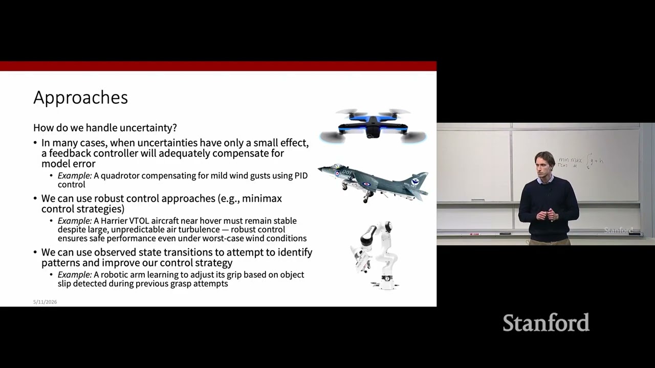
[02:50](https://www.youtube.com/watch?v=RtJSHiqOdgQ&t=170s) Handling System Uncertainty: Three Paradigms

In a standard closed-loop control architecture, a controller sends control inputs to a physical system, sensors measure the resulting output states, and these measurements are compared against an intended reference behavior to generate error signals that drive subsequent control actions. In real-world engineering, however, systems inevitably suffer from unmodeled dynamics, external disturbances, and environmental parameter shifts. To address these discrepancies, three macro-level engineering strategies exist:

```mermaid flowchart TD accTitle: Three Paradigms for Handling Uncertainty accDescr: Overview of feedback compensation, robust min-max control, and data-driven learning. U["Uncertainty / Unmodeled Effects"] --> P1["1. Standard Feedback Control (Compensate via Error Tracking, e.g., PID)"] U --> P2["2. Robust Adversarial Control (Min-Max Optimization over Worst-Case Disturbance)"] U --> P3["3. Data-Driven Learning (Collect State Transitions to Learn Models/Policies)"] ```

1. **Simple Feedback Compensation:** When unmodeled dynamics exert only minor influences on system behavior—such as a multirotor drone encountering gentle, unmodeled wind gusts—sophisticated adaptation may be unnecessary. A well-tuned feedback controller (such as a PID loop tracking a reference flight trajectory) often provides sufficient corrective authority to counteract the disturbance directly. 2. **Robust and Adversarial Control:** When uncertainties are larger or safety-critical, one can formulate the control task as a game-theoretic min-max optimization problem. Here, the controller seeks to maximize a performance reward or minimize cost with respect to the control input $u$, while an adversary draws disturbances from an uncertainty set $\Gamma$ representing the worst-case scenario. While effective—evoking classic differential games like Rufus Isaacs' "homicidal chauffeur" problem discussed earlier in the semester—this paradigm tends to yield behaviors that are excessively conservative, defensive, and sub-optimal under nominal operating conditions. 3. **Data-Driven and Learning-Based Control:** Instead of preparing for an extreme worst-case adversary, this approach leverages empirical operational data. By logging previous trajectories, state transitions, and flight data from past missions, an agent learns an approximate model of the real dynamics or refines its control laws directly from observed data.

[07:44](https://www.youtube.com/watch?v=RtJSHiqOdgQ&t=464s) What to Learn: Direct vs. Indirect Learning Frameworks

When committing to data-driven methods, the primary design choice concerns the target of the learning process. The vast spectrum of learning-based control algorithms splits broadly into two foundational categories:

```mermaid flowchart LR accTitle: Direct vs Indirect Learning accDescr: Contrast between direct policy improvement from data and indirect model learning followed by controller synthesis. subgraph DirectApproach["Direct Control Improvement"] D1["Empirical Data / Transitions"] --> D2["Direct Policy Optimization"] D2 --> D3["Improved Controller"] end subgraph IndirectApproach["Indirect Model-Based Improvement"] I1["Empirical Data / Transitions"] --> I2["System Identification / Model Learning"] I2 --> I3["Approximate Dynamics Model"] I3 --> I4["Synthesize Controller"] end ```

- **Direct Methods:** Empirical observations, state transitions, and rollouts are fed directly into the policy optimization objective to improve control actions without ever constructing an explicit intermediate model of the plant dynamics. This paradigm encompasses direct adaptive control (such as Model Reference Adaptive Control), imitation learning, and model-free reinforcement learning. - **Indirect Methods:** Empirical measurements are first used to solve an intermediate system identification problem, fitting an approximate mathematical model of the system's dynamics. This surrogate model is then provided to an optimal control framework (such as MPC or LQR) to synthesize or update the controller. This family includes indirect adaptive control (such as Model Identification Adaptive Control) and model-based reinforcement learning.

[09:12](https://www.youtube.com/watch?v=RtJSHiqOdgQ&t=552s) Learning Regimes: The Zero-Episodes Setting

Beyond what is learned, algorithms differ fundamentally in *how* learning data is gathered and utilized during the system's operational lifecycle. The lecture introduces three prototypical learning regimes, beginning with the **zero-episodes case** (commonly referred to as classical offline system identification).

In the zero-episodes setting, no real-time policy updates or online learning occur while the system executes its live task. Instead, the engineer relies entirely on an offline, pre-collected dataset of state transitions or rollouts gathered under a prior logging policy or through dedicated exploratory experiments. This historical offline dataset is used to identify the underlying dynamics model or to tune a controller before deployment, ensuring that the control policy remains fixed once operational execution begins.

- The zero-episodes regime treats model training as a purely offline prerequisite, eliminating the stability risks associated with updating controllers in real time during execution. - The pre-collected offline dataset forms the basis for either directly optimizing control parameters or fitting state-space matrices and nonlinear dynamics functions via regression.

[10:00](https://www.youtube.com/watch?v=RtJSHiqOdgQ&t=600s) Modalities of Experience: Zero, One, and Multiple Episodes

Dr. Daniele Gammelli distinguishes three primary operational settings or "modalities of experience" when integrating learning into control systems: zero-episode, one-episode, and multiple-episode learning. In the zero-episode paradigm, an agent relies on an offline dataset collected beforehand. This fixed collection of past data is used offline to estimate unknown parameters or train predictive dynamical models, which are then frozen and deployed to optimize controller performance.

The one-episode setting represents online adaptation. In this regime, learning and adaptation must occur on the fly while actively controlling the system in real time, with no luxury of prior flight datasets to lean on. To illustrate, Gammelli revisits the quadrotor example: suppose a drone must carry a payload of unknown mass $m$. Under an online adaptation framework, the system cannot estimate this mass from previous flights. Instead, while actively stabilizing and steering the drone in the air, the controller must concurrently estimate the unknown mass $m$ and adapt its control commands before the vehicle destabilizes.

The third category is the multiple-episode framework, which forms the classical foundation of reinforcement learning (RL). Here, an agent interacts with an environment that can be reset indefinitely. Gammelli points to chess as an intuitive analogy: the chess board represents an environment where an agent attempts to learn an optimal policy. The game spawns at an initial state, the agent plays through a full sequence of moves until an episode concludes, the board resets, and the agent uses performance feedback accumulated across successive games to iteratively refine its policy parameters.

While these categories provide a clear taxonomy, Gammelli cautions that the boundaries are not completely rigid: offline reinforcement learning, for instance, technically optimizes RL objectives yet operates entirely within the zero-episode offline dataset regime. The choice of algorithm ultimately hinges on what experience is accessible: an offline dataset collected in advance, real-time closed-loop operation requiring instant adaptation, or an interactive simulator/environment that can be reset repeatedly.

```mermaid flowchart TD accTitle: Modalities of Experience in Learning-Based Control accDescr: Diagram illustrating zero episode, one episode, and multiple episode modalities with examples.

subgraph ZeroEp["Zero Episode (Offline)"] D0["Static Offline Dataset"] --> M0["Train Model / Estimate Params"] M0 --> C0["Deploy Frozen Controller"] end

subgraph OneEp["One Episode (Online Adaptation)"] D1["Real-Time Execution"] -->|"Concurrent Estimation"| M1["Adapt Params (e.g., Unknown Mass m)"] M1 -->|"Immediate Feedback"| D1 end

subgraph MultiEp["Multiple Episodes (Reinforcement Learning)"] E2["Episode Interaction"] -->|"Termination & Reset"| U2["Policy Update Across Games"] U2 --> E2 end ```

[12:15](https://www.youtube.com/watch?v=RtJSHiqOdgQ&t=735s) Student Q&A: Exploration, Policy-Driven Data, and Trajectory Chunking

A student asks for clarification on the boundary between one-episode and multiple-episode settings, asking whether the defining factor of multiple episodes is simply the ability to interact with the environment and learn from those interactions. Gammelli clarifies that online one-episode controllers also interact directly with their environment; the critical distinction lies in the *episodic nature* and resets across repeated trials. Returning to the chess analogy, multi-episode learning is akin to playing thousands of separate games to master strategy over time, whereas one-episode learning is equivalent to being thrown into a single ongoing game and trying to learn how to play chess while actively making moves to avoid losing.

Another student observes that multiple episodes allow an agent to reach states that a single run might never explore, and asks how this applies to vehicle trajectory data: if an engineer deploys an instrumented vehicle, records a long time history, and slices that single recording into multiple shorter time horizons, does that count as multiple episodes?

Gammelli explains that slicing up a pre-recorded piloted trajectory actually belongs to the zero-episode (offline) regime:

> "I would probably classify this in the zero episode case, meaning that you have a dataset of trajectories and you're basically chunking this up in order to build a kind of next-state prediction or a forward dynamics problem... because you're not really being necessarily an agent in collecting that data."

In true multiple-episode reinforcement learning, the system's own evolving policy dictates the data collection and exploration path. In physical robotics, this highlights why zero-episode offline learning is so heavily favored over tabular or trial-and-error RL: you cannot deploy a randomly initialized neural network from scratch to drive an autonomous vehicle on open roads because "this will crash for sure." In a simulated game of chess, terrible initial policies carry zero real-world risk, allowing arbitrary exploration that physical hardware cannot tolerate.

[15:45](https://www.youtube.com/watch?v=RtJSHiqOdgQ&t=945s) System Identification via Least-Squares Linear Regression

With the taxonomy established, Gammelli transitions to classical approaches in learning-based control, beginning with system identification (SysID). SysID relies on the insight that many real-world control problems do not require online learning during deployment. Instead, engineers can run prior system tests, assemble an offline dataset of historical inputs and responses, fit a data-driven dynamics model, and insert that estimated model directly into standard model-based control synthesis (such as LQR or MPC) as a proxy for the unknown physics.

To formalize the mathematical foundation, Gammelli reviews standard linear regression via least-squares minimization. Consider a data-generating process where an output $y$ relates linearly to an input feature vector $z$ with unknown parameter vector $\theta$ and additive noise $\epsilon$:

$$y = \theta^T z + \epsilon$$

The learning objective is to estimate $\theta$ using an offline dataset $\mathcal{D}$ consisting of $N$ input-output observation pairs:

$$\mathcal{D} = \left\{(z_i, y_i)\right\}_{i=1}^N$$

Stacking the individual observations into target vector $Y \in \mathbb{R}^N$ and data matrix $Z \in \mathbb{R}^{N \times d}$, the least-squares performance criterion penalizes the squared Euclidean norm of prediction errors:

$$\min_{\theta} \|Y - Z\theta\|_2^2$$

Expanding this objective reveals a convex quadratic function in terms of $\theta$:

$$\|Y - Z\theta\|_2^2 = (Y - Z\theta)^T (Y - Z\theta) = Y^T Y - 2 \theta^T Z^T Y + \theta^T Z^T Z \theta$$

Because the objective is unconstrained and strictly convex (assuming $Z^T Z$ is invertible), the necessary and sufficient condition for optimality is that the gradient with respect to $\theta$ must vanish:

$$\nabla_{\theta} \left( Y^T Y - 2 \theta^T Z^T Y + \theta^T Z^T Z \theta \right) = -2 Z^T Y + 2 Z^T Z \theta = 0$$

Setting this gradient to zero yields the standard normal equations:

$$Z^T Z \theta = Z^T Y$$

Solving for $\theta$ gives the closed-form least-squares estimator:

$$\theta^* = (Z^T Z)^{-1} Z^T Y$$

- **Input vector $z_i$**: The regressor or feature vector for data point $i$. - **Output scalar/vector $y_i$**: The ground-truth measured response. - **Data matrix $Z$**: The matrix composed of row-stacked input vectors. - **Target vector $Y$**: The stacked vector of measured outputs. - **Parameter vector $\theta^*$**: The analytical minimum of the least-squares loss.

[20:10](https://www.youtube.com/watch?v=RtJSHiqOdgQ&t=1210s) Mapping Linear Regression to System Dynamics Identification

Gammelli takes the mathematical machinery of least squares and directly maps it onto the problem of learning unknown physical dynamics. Consider an unknown discrete-time linear dynamical system perturbed by noise:

$$x_{t+1} = A x_t + B u_t + w_t$$

Here, $x_t$ denotes the state at time $t$, $u_t$ represents the control input, and $w_t$ represents process noise or unmodeled disturbances. This relationship can be expressed compactly in linear regression form by concatenating the state and control into a single input vector, and grouping the unknown system matrices into a parameter block:

$$x_{t+1} = \begin{bmatrix} A & B \end{bmatrix} \begin{bmatrix} x_t \\ u_t \end{bmatrix} + w_t$$

Gammelli directly maps each dynamical variable to the regression notation: - The measured output $y$ corresponds to the next state transition $x_{t+1}$. - The regression input $z$ corresponds to the combined state-action pair $\begin{bmatrix} x_t \\ u_t \end{bmatrix}$. - The parameter vector/matrix $\theta$ corresponds to the stacked dynamics matrices $\begin{bmatrix} A & B \end{bmatrix}^T$.

In practice, acquiring this regression data requires running the system (or a human operator piloting it) through a series of rollouts or trajectories over time. Each trajectory is an ordered time history of visited states and applied control commands:

$$\tau = (x_0, u_0, x_1, u_1, \dots, x_T)$$

From these historical trajectories, the dataset $\mathcal{D}$ is constructed by extracting consecutive one-step transition tuples:

$$\mathcal{D} = \left\{ \left( (x_t, u_t), \, x_{t+1} \right) \right\}$$

Each observed pair of current state $x_t$ and applied control $u_t$ serves as the input $z_i$, and the resulting subsequent state $x_{t+1}$ serves as the target label $y_i$. By populating matrices $Z$ and $Y$ with these transition pairs across all available trajectories, the optimal system matrices $\begin{bmatrix} \hat{A} & \hat{B} \end{bmatrix}$ are identified directly via linear regression.

[25:00](https://www.youtube.com/watch?v=RtJSHiqOdgQ&t=1500s) Ordinary Least Squares and the Estimator as a Random Variable

Dr. Daniele Gammelli recaps how system dynamics can be approximated directly from data. The process relies on collecting trajectories of the system's evolution and repurposing those observations into a regression problem that maps the current state and control action to the next state. Addressing the practical implementation of the ordinary least squares (OLS) solution, he highlights that the formula involves computing $(Z^\top Z)^{-1}$. When data matrices grow massive, inverting this matrix directly becomes computationally prohibitive. To handle continuous incoming streams of data without performing costly matrix inversions at every time step, one can turn to recursive formulations (such as recursive least squares), which have equivalents in both discrete and continuous time.

```mermaid flowchart LR accTitle: System Identification via Least Squares accDescr: Pipeline showing data collection mapping to regression, OLS parameter estimation, and evaluation via statistical properties. subgraph DataCollection["Data Collection"] D["Trajectories: (x_t, u_t) → x_{t+1}"] Z["Feature Matrix Z"] D --> Z end subgraph Estimation["Parameter Estimation"] OLS["OLS Solution: (Z^T Z)^{-1} Z^T Y"] RLS["Recursive Formulations\n(avoid large inversions)"] Z --> OLS OLS -.-> RLS end subgraph StatisticalAnalysis["Statistical Analysis"] BLUE["BLUE / MLE Properties"] RV["Random Variable: Mean & Covariance"] OLS --> BLUE OLS --> RV end ```

He then reviews classical theoretical guarantees for the least-squares estimator: - Under standard noise assumptions where the noise terms $\epsilon_t$ are zero-mean, uncorrelated, and exhibit identical, finite variance, the estimator is the **Best Linear Unbiased Estimator (BLUE)**. - If the disturbance distribution is specifically Gaussian, the derived least-squares estimator matches the **Maximum Likelihood Estimator (MLE)**.

Moving deeper into the convergence properties, Dr. Gammelli poses the central question: under what sufficient conditions does the parameter estimate $\hat{\theta}$ converge to the true parameter vector $\theta^*$ as the volume of collected data increases? Visualizing data quantity on the x-axis and the estimate $\hat{\theta}$ on the y-axis, the goal is to determine whether the estimate centers on $\theta^*$ and how its spread shrinks. Because the measurement vector depends on additive noise ($Y = Z \theta + \epsilon$), substituting this expression back into the estimator yields:

$$\hat{\theta} = \theta + (Z^\top Z)^{-1} Z^\top \epsilon$$

Because the noise vector $\epsilon$ is stochastic, the parameter estimate $\hat{\theta}$ is itself a random variable. Consequently, evaluating its convergence requires analyzing its statistical moments—specifically its mean and covariance.

---

[30:00](https://www.youtube.com/watch?v=RtJSHiqOdgQ&t=1800s) Convergence Analysis: Expectation, Covariance, and Persistent Excitation

Dr. Gammelli inspects the expected value of $\hat{\theta}$. Applying the expectation operator $\mathbb{E}[\hat{\theta}] = \mathbb{E}[\theta + (Z^\top Z)^{-1} Z^\top \epsilon]$, the deterministic matrices pull outside the expectation. Since the disturbance sequence satisfies the zero-mean assumption ($\mathbb{E}[\epsilon] = 0$), the right-hand error term drops out entirely, leaving:

$$\mathbb{E}[\hat{\theta}] = \theta$$

This confirms that the estimator is strictly unbiased: in expectation, collecting more data centers the estimate precisely on the ground-truth parameter values.

Next, he analyzes the covariance to determine whether estimation uncertainty contracts around the true parameters. Applying the covariance identity $\operatorname{Cov}(Ax) = A \operatorname{Cov}(x) A^\top$, with $A = (Z^\top Z)^{-1} Z^\top$ and $x = \epsilon$, the covariance matrix of $\epsilon$ is simplified. Because the disturbances are assumed to be uncorrelated with equal variance $\sigma^2$, $\operatorname{Cov}(\epsilon)$ reduces to a diagonal matrix $\sigma^2 I$. Pushing the algebra through yields:

$$\operatorname{Cov}(\hat{\theta}) = \sigma^2 \left( \sum_{t=1}^n z_t z_t^\top \right)^{-1}$$

where $z_t$ contains the combinations of observed states and control inputs. For the covariance to diminish toward zero as $n \to \infty$, the summation term inside the inverse must grow unboundedly toward infinity. This condition hinges on operating the system in a non-trivial manner rather than remaining stationary at the origin. Dr. Gammelli formalizes this concept as **persistent excitation**: the inputs must continuously probe the system in rich, informative directions so that the inverted sum vanishes and $\hat{\theta}$ converges with zero variance to $\theta^*$.

---

[35:00](https://www.youtube.com/watch?v=RtJSHiqOdgQ&t=2100s) Practical Challenges: Model Accuracy vs. Control Performance

An audience member asks about the distribution support and invertibility regularity conditions. Dr. Gammelli acknowledges that rigorous mathematical treatments include explicit regularity conditions guaranteeing invertibility, but emphasizes that the primary purpose here is establishing the control intuition: under linear assumptions and persistent excitation, system identification yields unbiased estimates that converge with zero asymptotic covariance.

He then steps back to address the core dilemmas of system identification in practical control: - **Data Budget & Sample Complexity**: How many data points are realistically needed to learn a viable dynamics model, and how should parameter estimation quality be quantified? - **Mismatch Between Identification and Control**: In classical statistics, parameter estimation accuracy (e.g., small parameter distance $\|\hat{\theta} - \theta^*\|$) is the sole metric. In robotics and control, however, practitioners only care about controller closed-loop performance: "We do not really care too much about model accuracy. What we care about is that we get a better controller out of this process." - **Threshold Effects**: Dr. Gammelli sketches a scenario where a control law switches discontinuously based on the sign of a parameter $\theta$ (e.g., one control action if $\theta < 0$, a different one if $\theta > 0$). If the ground-truth parameter is slightly positive, an estimate $\hat{\theta}_1$ might be numerically closer to $\theta^*$ but land on the negative side of zero, triggering the wrong control action. Meanwhile, a second estimate $\hat{\theta}_2$ could be further away in Euclidean distance yet share the correct positive sign, yielding vastly superior closed-loop performance. This reveals a fundamental limitation of standard system identification: fitting model parameters acts as an intermediate surrogate objective that is not strictly aligned with downstream control success. - **Active Data Collection & Safety**: Real-world data is collected online while the robot is running. Operating with an incomplete or uncertain model introduces severe risks, necessitating cautious, conservative exploration. - **Model Expressivity vs. Capacity**: The derivations assume the real system matches the linear parameterization. If the underlying dynamics contain nonlinearities outside this hypothesis class, one faces a structural trade-off between model expressivity, sample efficiency, and model misspecification.

[40:00](https://www.youtube.com/watch?v=RtJSHiqOdgQ&t=2400s) The Adaptive Control Paradigm: Online Adaptation and Coupled Stability

Dr. Gammelli bridges the transition from system identification to adaptive control by contrasting their learning regimes. While system identification primarily operates in an offline, "zero episodes" setting—where a fixed dataset is collected to estimate dynamics models before synthesizing a controller—adaptive control is inherently a "one episode" problem. In adaptive control, the agent must refine its behavior online in real time while actively operating the physical system. This online learning paradigm bifurcates into two standard methodologies: directly tuning the controller's internal parameters on the fly, or continuously updating an estimated dynamics model and leveraging that updated model to adjust the control policy. This distinction underpins the division between Model Reference Adaptive Control (MRAC), which directly adjusts the controller, and Model Identification Adaptive Control (MIAC), which identifies a model to improve control performance.

```mermaid flowchart TD accTitle: Adaptive Control Taxonomy accDescr: Flowchart contrasting Model Reference Adaptive Control and Model Identification Adaptive Control in an online setting. subgraph OnlineAdaptation["Online One-Episode Adaptive Control"] direction TB A["Online Operating Data"] --> B{"Control Adaptation Strategy"} B -->|"Direct Parameter Update"| C["Model Reference Adaptive Control (MRAC)"] B -->|"Indirect via Dynamics Estimation"| D["Model Identification Adaptive Control (MIAC)"] C --> E["Directly Adjusted Controller"] D --> F["Updated System Model"] --> E end ```

The instructor stresses that classical adaptive control literature, dating back decades, differs fundamentally from modern optimal control. Rather than optimizing an objective cost function or performance metric, traditional adaptive control revolves strictly around certifying the stability of the coupled closed-loop system. When deploying adaptive techniques, three components are inherently linked in a feedback loop: the physical system dynamics, the parameterized feedback controller, and the adaptation law driving parameter updates. Consequently, the primary theoretical mission is not minimizing a cost functional, but designing the controller and adaptation dynamics such that the entire coupled system remains provably stable.

- **Offline vs. Online Learning:** System identification uses pre-collected data (zero episodes) to build a static model, whereas adaptive control adapts within a single continuous operational run (one episode). - **Direct vs. Indirect Approaches:** MRAC tunes controller gains directly; MIAC estimates plant dynamics parameters first and subsequently recalculates control inputs. - **Stability-Centric Objective:** Instead of solving an optimization problem for a cost metric, classical adaptive control focuses on verifying stability guarantees for the coupled triadic interaction: plant dynamics + feedback controller + adaptation rule.

---

[42:47](https://www.youtube.com/watch?v=RtJSHiqOdgQ&t=2567s) Tool of Choice: Global Asymptotic Stability via Lyapunov's Direct Method

To establish rigorous stability proofs for these coupled systems, the course relies on Lyapunov stability theory. Dr. Gammelli recalls the formulation for an autonomous system $\dot{x} = f(x)$, noting that controlled systems driven by a feedback policy $u = \pi(x)$ fit directly into this framework because the control input can be subsumed into the closed-loop autonomous dynamics $\dot{x} = f(x, \pi(x))$. Assuming an equilibrium point $x^*$ satisfies $f(x^*) = 0$, Lyapunov's direct method provides an analytical shortcut to certify stability without needing to integrate nonlinear differential equations or evaluate trajectories across every possible initial state.

Building on the local stability concepts introduced in previous lectures, Dr. Gammelli details the three rigorous conditions required for a scalar candidate function $V(x)$ to establish *global* asymptotic stability:

1. **Positive Definiteness:** $V(x) > 0$ for all $x \neq x^*$, and $V(x^*) = 0$. 2. **Negative Definiteness of the Derivative:** Along system trajectories, $\dot{V}(x) < 0$ for all $x \neq x^*$. 3. **Radial Unboundedness:** As the state norm grows arbitrarily large, the Lyapunov function must diverge: $$\lim_{\|x\| \to \infty} V(x) = \infty$$

Dr. Gammelli paints a visual picture of this mathematical construct as an open, "ball-shaped" bowl centered at the origin in the state space $(x_1, x_2)$. As the system trajectories unfold, the value of $V(x)$ monotonically dissipates down the contours of the bowl, driving the state inexorably to the minimum at the equilibrium point. Radial unboundedness ensures that the bowl's walls extend to infinity in every direction, preventing trajectories from escaping to infinity along paths where the energy function might otherwise remain bounded.

---

[46:42](https://www.youtube.com/watch?v=RtJSHiqOdgQ&t=2802s) Tutorial Example: Lyapunov Stability of a Mass-Spring-Damper

Before applying Lyapunov theory to adaptive control architectures, Dr. Gammelli steps through a foundational physics example to demonstrate the mechanics of the proof: an unforced, passive mass-spring-damper system. The system comprises a mass $m$, a spring with stiffness $k$, and a viscous damper with damping coefficient $d$. The state vector consists of position and velocity, $(x, \dot{x})$, with the desired equilibrium located at the origin $(0, 0)$—zero position and zero velocity.

The candidate Lyapunov function is chosen as the total mechanical energy of the physical system, combining elastic potential energy and kinetic energy:

$$E(x, \dot{x}) = \frac{1}{2} k x^2 + \frac{1}{2} m \dot{x}^2$$

By inspection, conditions 1 and 3 are readily satisfied: the quadratic sum is strictly positive everywhere away from the origin, vanishes at $(0,0)$, and grows without bound as the position or velocity approaches infinity. The core analytical task is therefore evaluating the second condition by differentiating the energy candidate with respect to time along the system trajectories:

$$\dot{E}(x, \dot{x}) = k x \dot{x} + m \dot{x} \ddot{x}$$

From Newton's second law, the equation of motion for the system is $m \ddot{x} = -d \dot{x} - k x$. Substituting this relationship into the acceleration term yields:

$$\dot{E}(x, \dot{x}) = k x \dot{x} + \dot{x}(-d \dot{x} - k x) = k x \dot{x} - d \dot{x}^2 - k x \dot{x} = -d \dot{x}^2$$

The conservative spring terms $k x \dot{x}$ cancel out completely, isolating the dissipative effect of the damper: $\dot{E} = -d \dot{x}^2 \le 0$. This confirms that energy dissipates whenever velocity is nonzero, validating the power of Lyapunov analysis to certify system stability directly from the governing physics without explicitly solving the differential equation.

---

[50:18](https://www.youtube.com/watch?v=RtJSHiqOdgQ&t=3018s) Model Reference Adaptive Control (MRAC) Framework and Setup

Returning to the main focus of the lecture, Dr. Gammelli formalizes the architecture of Model Reference Adaptive Control (MRAC). The MRAC formulation relies on four foundational components:

1. **The Plant:** The underlying physical system to be controlled, containing unknown or uncertain parameters. 2. **The Reference Model:** An idealized dynamical system that outputs the desired reference response $x_m$. Dr. Gammelli emphasizes that the reference model serves as an implicit surrogate for performance: instead of defining a classical cost function to minimize, performance is quantified directly by the tracking error between the actual plant output and this reference trajectory. 3. **The Feedback Controller:** A parameterized control policy designed with tunable, adjustable gains. 4. **The Adaptation Mechanism:** The differential or difference equation that specifies exactly how the controller's adjustable gains evolve over time in response to observed tracking errors.

To make the theoretical analysis concrete, Dr. Gammelli outlines the pedagogical strategy: the class will first study the nominal tracking problem where the plant's physical parameters are assumed to be completely known, deriving a baseline tracking controller. Once this baseline is established, they will strip away the assumption of known parameters, introduce real-time adaptation laws, and re-apply Lyapunov techniques to prove stability for the fully coupled, parameter-adaptive closed-loop system.

The setup begins with a canonical double integrator plant representing a point mass driven by an input force:

$$m \ddot{x} = u$$

To dictate how this mass ought to move, a fictitious reference model state $x_m$ is introduced, driven by an external positioning command to establish the target trajectory that the true state $x$ must track.

[55:00](https://www.youtube.com/watch?v=RtJSHiqOdgQ&t=3300s) Reference Model and Nominal Tracking Controller

Dr. Daniele Gammelli introduces the reference model that describes the ideal, target response of the controlled mass. To specify this desired behavior, a fictitious state $x_m$ (where subscript $m$ denotes "model") is introduced, governed by a second-order linear differential equation:

$$\ddot{x}_m + k_d \dot{x}_m + k_p x_m = k_r r(t)$$

Here, $x_m$ is the ideal output, the parameters $k_d$, $k_p$, and $k_r$ are design gains chosen by the control engineer, and $r(t)$ is an externally provided reference positioning command.

Before tackling uncertainty, the ideal baseline case is considered: suppose the mass $m$ is known exactly. In this scenario, perfect tracking of the reference model can be achieved using a model-canceling control law:

$$u = m \left( \ddot{x}_m - 2\lambda \dot{\tilde{x}} - \lambda^2 \tilde{x} \right)$$

where $\tilde{x} = x - x_m$ is defined as the tracking error between the actual system position $x$ and the ideal reference position $x_m$, and $\lambda > 0$ is a strictly positive control gain chosen by the designer.

Gammelli steps back to reflect on the methodology of adaptive control design. Students often wonder where such reference models and control equations come from. In practical engineering, designing these components is an iterative craft: an engineer hypothesizes a reference model suitable for the hardware, tests a candidate control law, checks whether stability can be proven, and refines the design if the proof fails. In the lecture, however, these structures are given up front to demonstrate the rigorous stability analysis that validates them.

```mermaid flowchart LR accTitle: Nominal Reference-Model Tracking Pipeline accDescr: Reference command drives the reference model, and the tracking error between plant output and model output feeds into the nominal control law. subgraph Target["Reference Model"] R["Reference r(t)"] --> RM["Model: x_m, x_m_dot, x_m_ddot"] end subgraph Error["Error Formation"] RM --> DIFF["Tracking Error: x_tilde = x - x_m"] PLANT["Plant Mass m"] --> DIFF end subgraph Control["Nominal Feedback"] DIFF --> U["Control u = m(x_m_ddot - 2*lambda*x_tilde_dot - lambda^2*x_tilde)"] U --> PLANT end ```

[01:00:00](https://www.youtube.com/watch?v=RtJSHiqOdgQ&t=3600s) Closed-Loop Dynamics and Exponential Convergence Under Known Mass

To prove that the nominal controller guarantees exponential tracking, Dr. Gammelli derives the closed-loop error dynamics starting from the Newton's second law dynamics of the mass:

$$m \ddot{x} = u$$

Substituting the nominal control law into the plant dynamics yields:

$$m \ddot{x} = m \left( \ddot{x}_m - 2\lambda \dot{\tilde{x}} - \lambda^2 \tilde{x} \right)$$

Rearranging all terms onto one side gives:

$$m \left( \ddot{x} - \ddot{x}_m + 2\lambda \dot{\tilde{x}} + \lambda^2 \tilde{x} \right) = 0$$

Since $\ddot{x} - \ddot{x}_m = \ddot{\tilde{x}}$ and $m > 0$, the mass cancels out entirely, leaving a second-order linear ordinary differential equation for the tracking error:

$$\ddot{\tilde{x}} + 2\lambda \dot{\tilde{x}} + \lambda^2 \tilde{x} = 0$$

This ODE has a repeated negative root at $-\lambda$. Its general analytical solution is:

$$\tilde{x}(t) = (c_0 + c_1 t) e^{-\lambda t}$$

Because the designer chooses $\lambda > 0$, the exponential term decays faster than linear growth, meaning $\lim_{t \to \infty} \tilde{x}(t) = 0$. Since $\tilde{x} = x - x_m$, this guarantees that the actual trajectory asymptotically tracks the reference model perfectly over time.

Having established this nominal baseline, Gammelli shifts focus to the core topic of the lecture: the realistic setting where the physical mass $m$ is completely unknown, requiring an online estimate $\hat{m}(t)$. To keep the ensuing algebra clean, three auxiliary variables are introduced: - A filtered tracking error metric: $s = \dot{\tilde{x}} + \lambda \tilde{x}$ - A nominal acceleration command signal: $\nu = \ddot{x}_m - 2\lambda \dot{\tilde{x}} - \lambda^2 \tilde{x}$ - The parameter estimation error: $\tilde{m} = \hat{m} - m$, which implies $\hat{m} = \tilde{m} + m$

Evaluating the plant dynamics $m \ddot{x} = u$ using the certainty-equivalence controller $u = \hat{m}\nu$ yields:

$$m \ddot{x} = \hat{m}\nu = (m + \tilde{m})\nu = m\nu + \tilde{m}\nu$$

[01:05:00](https://www.youtube.com/watch?v=RtJSHiqOdgQ&t=3900s) Error Dynamics with Unknown Mass and the Parameter Adaptation Law

Rearranging the open equation $m \ddot{x} = m \nu + \tilde{m}\nu$ into closed-loop form gives:

$$m (\ddot{x} - \nu) = \tilde{m}\nu$$

Expanding the definition of $\nu$ inside the parenthesis:

$$m \left( \ddot{x} - \ddot{x}_m + 2\lambda \dot{\tilde{x}} + \lambda^2 \tilde{x} \right) = \tilde{m}\nu$$

Noticing that $\ddot{x} - \ddot{x}_m = \ddot{\tilde{x}}$, the term in brackets simplifies directly in terms of the composite variable $s$:

$$\dot{s} + \lambda s = \frac{d}{dt}(\dot{\tilde{x}} + \lambda \tilde{x}) + \lambda(\dot{\tilde{x}} + \lambda \tilde{x}) = \ddot{\tilde{x}} + 2\lambda \dot{\tilde{x}} + \lambda^2 \tilde{x}$$

Thus, the coupled error dynamics can be written compactly as:

$$m(\dot{s} + \lambda s) = \tilde{m}\nu$$

Because $m$ is unknown, an adaptation rule is required to update $\hat{m}$ in real time. Dr. Gammelli introduces the gradient-like parameter adaptation law:

$$\dot{\hat{m}} = -\gamma \nu s$$

where $\gamma > 0$ is a strictly positive adaptation gain chosen by the designer.

With the plant error dynamics and the parameter update law in place, Gammelli sets up a Lyapunov stability analysis to prove that the coupled state converges asymptotically to the desired equilibrium. He introduces the composite Lyapunov candidate function:

$$V(s, \tilde{m}) = \frac{1}{2} m s^2 + \frac{1}{2\gamma} \tilde{m}^2$$

This function penalizes both the tracking error metric $s$ and the parameter estimation error $\tilde{m}$. The first and third Lyapunov conditions ($V(0) = 0$ and $V(z) > 0$ for all $z \neq 0$, along with radial unboundedness) are straightforward to satisfy. The primary challenge is verifying the second condition: ensuring that the time derivative $\dot{V}$ is negative semi-definite along system trajectories.

Differentiating $V$ with respect to time gives:

$$\dot{V} = m s \dot{s} + \frac{1}{\gamma} \tilde{m} \dot{\tilde{m}}$$

Because the true mass $m$ is a constant physical parameter, $\dot{m} = 0$, which implies that the rate of change of the estimation error matches the adaptation rate:

$$\dot{\tilde{m}} = \frac{d}{dt}(\hat{m} - m) = \dot{\hat{m}}$$

[01:10:00](https://www.youtube.com/watch?v=RtJSHiqOdgQ&t=4200s) Lyapunov Proof and Sliding Line Phase-Plane Convergence

Substituting $\dot{\tilde{m}} = \dot{\hat{m}} = -\gamma \nu s$ into the derivative of the Lyapunov function gives:

$$\dot{V} = m s \dot{s} + \frac{1}{\gamma} \tilde{m} (-\gamma \nu s) = s (m \dot{s} - \tilde{m}\nu)$$

From the derived coupled error dynamics, $m(\dot{s} + \lambda s) = \tilde{m}\nu$, which can be rearranged as:

$$m \dot{s} - \tilde{m}\nu = -m \lambda s$$

Substituting this relation directly back into the expression for $\dot{V}$ produces the result:

$$\dot{V} = s (-m \lambda s) = -m \lambda s^2$$

Because the physical mass satisfies $m > 0$ and the control designer specifies $\lambda > 0$, the product $m \lambda$ is strictly positive. Therefore:

$$\dot{V} = -m \lambda s^2 \le 0$$

This confirms that $\dot{V}$ is negative semi-definite, guaranteeing that the composite error metric $s$ converges asymptotically to zero ($s \to 0$ as $t \to \infty$).

Dr. Gammelli then unpacks the physical and geometric meaning of $s \to 0$ in the error phase plane $(\tilde{x}, \dot{\tilde{x}})$. Recalling the definition $s = \dot{\tilde{x}} + \lambda \tilde{x}$, driving $s$ to zero forces the tracking error onto a stable line:

$$\dot{\tilde{x}} = -\lambda \tilde{x}$$

Gammelli illustrates the phase-plane behavior along this line: - Any arbitrary trajectory first collapses toward the line $\dot{\tilde{x}} = -\lambda \tilde{x}$ as $s \to 0$. - Once constrained to this line, if the position error $\tilde{x}$ is negative, its derivative $\dot{\tilde{x}} = -\lambda \tilde{x}$ is positive, driving the error up toward zero. - Conversely, if $\tilde{x}$ is positive, its derivative $\dot{\tilde{x}}$ is negative, driving the error down toward zero.

Thus, the phase trajectory slides directly into the origin $(0, 0)$. Since $\lim_{t \to \infty} \tilde{x}(t) = 0$, the plant position $x(t)$ successfully tracks the desired reference model $x_m(t)$, proving that the adaptive control scheme achieves model tracking even when the true mass is completely unknown.

[01:15:00](https://www.youtube.com/watch?v=RtJSHiqOdgQ&t=4500s) Proving Global Asymptotic Stability via Lyapunov Functions

Dr. Daniele Gammelli clarifies a student's question regarding how Lyapunov stability theory was applied in the preceding derivation to establish equilibrium point stability. He explains that they selected a candidate Lyapunov function formulated primarily in terms of the sliding variable or tracking error metric $s$. While the lecture explicitly verified the second of three core Lyapunov properties on the board, the remaining conditions can be satisfied straightforwardly, often through direct inspection. Once the candidate Lyapunov function satisfies all three requisite conditions, the Lyapunov stability theorem guarantees that the system is globally asymptotically stable with respect to its equilibrium point.

In the context of the robotic manipulator or tracking problem discussed, establishing this stability implies that $s$ converges asymptotically to zero globally. Dr. Gammelli emphasizes that the subsequent step of the analysis connects $s \to 0$ directly to the physical tracking error vanishing ($e \to 0$). Rather than relying on heuristics, the entire derivation operates as a clean, direct application of the classical Lyapunov stability theorem to guarantee asymptotic tracking performance.

[01:16:32](https://www.youtube.com/watch?v=RtJSHiqOdgQ&t=4592s) The Coupled Architecture of Adaptive Control

Addressing a follow-up question on parameter tuning and how convergence holds both when mass $M$ is known versus when it is unknown, Dr. Gammelli steps back to contextualize the overarching adaptive control framework. Classically, adaptive control requires synthesizing and proving the stability of a coupled tripartite system: the plant dynamics, the feedback controller, and an online adaptation mechanism that continuously tunes adjustable parameter estimates (such as the unknown mass $\hat{M}$).

```mermaid flowchart LR accTitle: Coupled Adaptive Control System Architecture accDescr: Block diagram illustrating the interaction between the plant system, feedback controller, and adaptation mechanism.

subgraph ControlLoop["Adaptive Feedback Loop"] SYS["Plant System (Unknown Parameter M)"] CTRL["Feedback Controller (Control Law u)"] ADAPT["Adaptation Mechanism (Parameter Update Law)"]

The progression in class began with analyzing a baseline system where the parameter $M$ was assumed to be known, demonstrating stability under nominal state feedback. In the adaptive setting, an update law is added to adjust the estimate of $M$ online using dedicated adaptation gains ($\Gamma$ or $\lambda$). In practice, an engineer must tune these adaptation gains directly to achieve the desired transient behavior.

Dr. Gammelli acknowledges that students often find this material dense, intricate, and disorienting because multiple mathematical objects appear almost out of nowhere: - A customized control law designed to cancel out specific nonlinearities. - A virtual reference trajectory formulated to shape error dynamics. - An adaptation update law configured to update unknown mass parameters. - A candidate Lyapunov function crafted specifically to make negative-definiteness fall out cleanly.

He notes that designing these components from scratch is intensely case-specific. For this course, rather than getting bogged down in ad hoc derivations for every possible dynamical system, the pedagogical focus is deliberately placed on understanding the stability analysis that ties all these moving parts together once they are established.

[01:18:25](https://www.youtube.com/watch?v=RtJSHiqOdgQ&t=4705s) The Art of Finding Lyapunov Functions and Lecture Wrap-Up

A student presses on the core difficulty of this methodology: the entire proof relies entirely on finding that exact, specialized Lyapunov function—how does one actually discover it in real-world engineering? Dr. Gammelli smiles and admits that this is precisely where the lecture is "completely kind of fast tracking." He jokes that in control theory, coming up with a novel Lyapunov function for a complex, non-trivial system and rigorously proving its stability is not just routine homework—"if you have an interesting system and you derive a Lyapunov function and you show that the system is stable, you write a paper about it and you're happy about it."

Deriving candidate Lyapunov functions is famously an art that is heavily system-dependent. Throughout the lecture, they have been operating under the assumption that "either us, a previous version of us, or someone incredibly smart is giving us all of these things, and we just analyze it." He points students to the references listed on the upcoming slide to explore the forward-design synthesis methods used to construct these functions from first principles.

With class time expiring, Dr. Gammelli pauses the remaining discussion on Model Reference Adaptive Control (MRAC), promising to pick it up at the start of the next lecture before signing off.

## Notable quotes > [00:00](https://www.youtube.com/watch?v=RtJSHiqOdgQ&t=0s) which is basically a framework which tries to get the best of these two approaches — Dr. Daniele Gammelli

> [02:50](https://www.youtube.com/watch?v=RtJSHiqOdgQ&t=170s) homicidal chauffeur — Dr. Daniele Gammelli

> [10:00](https://www.youtube.com/watch?v=RtJSHiqOdgQ&t=600s) modalities of experience — Dr. Daniele Gammelli

> [12:15](https://www.youtube.com/watch?v=RtJSHiqOdgQ&t=735s) I would probably classify this in the zero episode case, meaning that you have a dataset of trajectories and you're basically chunking this up in order to build a kind of next-state prediction or a forward dynamics problem... because you're not really being necessarily an agent in collecting that data. — Dr. Daniele Gammelli

> [12:15](https://www.youtube.com/watch?v=RtJSHiqOdgQ&t=735s) this will crash for sure — Dr. Daniele Gammelli

> [35:00](https://www.youtube.com/watch?v=RtJSHiqOdgQ&t=2100s) We do not really care too much about model accuracy. What we care about is that we get a better controller out of this process. — Dr. Daniele Gammelli

> [42:47](https://www.youtube.com/watch?v=RtJSHiqOdgQ&t=2567s) ball-shaped — Dr. Daniele Gammelli

> [01:18:25](https://www.youtube.com/watch?v=RtJSHiqOdgQ&t=4705s) completely kind of fast tracking — Dr. Daniele Gammelli

> [01:18:25](https://www.youtube.com/watch?v=RtJSHiqOdgQ&t=4705s) if you have an interesting system and you derive a Lyapunov function and you show that the system is stable, you write a paper about it and you're happy about it. — Dr. Daniele Gammelli

> [01:18:25](https://www.youtube.com/watch?v=RtJSHiqOdgQ&t=4705s) either us, a previous version of us, or someone incredibly smart is giving us all of these things, and we just analyze it. — Dr. Daniele Gammelli

## Mentioned Dr. Daniele Gammelli, Prof. Marco Pavone, Rufus Isaacs, Stanford University, Department of Aeronautics and Astronautics, Stanford University, Italian Institute of Artificial Intelligence (AI4I), Center for Aerospace Autonomy Research (CAESAR), Center for Automotive Research at Stanford (CARS), Technical University of Denmark (DTU), NVIDIA, Principles of Robot Autonomy, AA203 Optimal and Learning-Based Control, Hamilton-Jacobi-Bellman (HJB), Hamilton-Jacobi-Isaacs (HJI), Model Reference Adaptive Control (MRAC), Model Identification Adaptive Control (MIAC), Model Predictive Control (MPC), Linear Quadratic Regulator (LQR), Best Linear Unbiased Estimator (BLUE), Maximum Likelihood Estimator (MLE), Lyapunov stability theory

## Video description Lecture 13 — Intro to Learning, System Identification, and Adaptive Control

Read the companion textbook, Principles of Robot Autonomy, free online: https://porabook.com

To learn more about enrolling in AA203 Optimal and Learning-Based Control, visit: https://online.stanford.edu/courses/aa203-optimal-and-learning-based-control

Follow along with the course schedule and syllabus: https://stanfordasl.github.io/aa203/sp2526/

Lecture slides: https://stanfordasl.github.io/aa203/sp2526/pdfs/lecture/lecture_3.pdf

Speaker: Dr. Daniele Gammelli

Bio: Dr. Daniele Gammelli is the Research Director of the Machine Intelligence for Robot Autonomy Laboratory at the Italian Institute of Artificial Intelligence (AI4I), and a Researcher in the Department of Aeronautics and Astronautics at Stanford University. Since 2022, he has been a Research Fellow at the Center for Aerospace Autonomy Research (CAESAR) at Stanford and, until 2025, at the Center for Automotive Research at Stanford (CARS). He received his Ph.D. in Machine Learning and Mathematical Optimization from the Technical University of Denmark (DTU) in 2022, where his doctoral thesis was nominated for the DTU Best Thesis of the Year Award and the DTU Young Researcher Award. Dr. Gammelli’s research focuses on developing the algorithmic foundations and system-level methodologies that enable AI-powered autonomous systems to operate safely, efficiently, and reliably in high-stakes environments, with an emphasis on aerospace autonomy and next-generation mobility systems.

Instructors: Prof. Marco Pavone, Associate Professor of Aeronautics and Astronautics, Director of Autonomous Vehicle Research at NVIDIA

Dr. Daniele Gammelli, Research Director at the Italian Institute of Artificial Intelligence (AI4I), Researcher at the Department of Aeronautics and Astronautics, Stanford University

Full playlist: https://www.youtube.com/playlist?list=PLa9dmHsLK9dg

#StanfordOnline #OptimalControl #Robotics #PhysicalAI

[Source](https://www.youtube.com/watch?v=RtJSHiqOdgQ)

中文简报

斯坦福Gammelli表明自适应控制优于单纯模型精度由于策略阈值效应，参数估计精度无法确保闭环控制的成功，因而需要通过耦合Lyapunov动力学而非精确对象模型来保障跟踪效果的自适应方案。 Daniele Gammelli博士标志着课程正式进入后半部分，研究重心从基于已知物理规律的最优控制转向应对未知或不确定动力学的基于学习的技术。本次课程建立了跨越零回合、单回合和多回合机制的学习分类体系，并演示了利用普通最小二乘回归进行的离线系统辨识以及持续激励的条件。随后转向在线单回合自适应，Gammelli博士展示了针对具有未知惯性质量系统的模型参考自适应控制（MRAC）。最后，讲座结合Lyapunov直接法与滑动线相平面分析，证明了被控对象、反馈控制器和梯度自适应律构成的耦合系统能够实现全局渐近跟踪。斯坦福AA203课程转向面向不确定动力学的基于学习的控制，从直接策略优化与间接系统辨识的对比，以及零回合（离线SysID）、单回合（在线自适应）和多回合（强化学习）机制的运行经验对各类方法进行了归类。 (0:00) 最小二乘系统辨识能够提供无偏线性模型，其协方差仅在持续激励下才会消失；然而，受参数阈值效应影响，最小化参数估计误差本质上并不能确保下游闭环控制的成功。 (30:00) 与最小化代价泛函的最优控制框架不同，经典自适应控制的核心在于论证被控对象动力学、反馈控制器以及在线参数自适应律三者之间耦合相互作用的稳定性。 (40:00) 对于质量未知的模型参考自适应控制（MRAC），将确定性等价控制律与类梯度参数更新律相结合可获得半负定的Lyapunov导数，从而沿稳定的滑动流形将滤波跟踪误差驱动至零。 (65:00)

Reading summary

Dr. Daniele Gammelli transitions the course from optimal control with known physical dynamics to learning-based control under uncertainty, contrasting offline system identification against real-time adaptive strategies like Model Reference Adaptive Control. Frameworks for Uncertainty and Experience Modalities (2:50) Engineering systems inevitably face unmodeled dynamics, which Gammelli groups into three management strategies: standard feedback compensation for minor disturbances, robust min-max formulations against worst-case adversaries, and data-driven learning. Within data-driven control, approaches split into direct policy optimization and indirect surrogate dynamics identification. These methods operate across three experience modalities: zero-episode (offline datasets), one-episode (real-time online adaptation), and multiple-episode (episodic interaction with resets, typical of reinforcement learning). While multi-episode reinforcement learning relies on risk-free environment resets like games of chess, Gammelli notes that safety-critical physical systems cannot tolerate the random exploration of early training policies without crashing. Consequently, physical robotics often relies either on zero-episode offline identification or tightly constrained one-episode online adaptation. System Identification Guarantees and Control Misalignment (15:45) In the zero-episode regime, unknown linear dynamics are cast into an ordinary least squares problem, yielding the closed-form estimator $\theta^* = (Z^T Z)^{-1} Z^T Y$. Under zero-mean, uncorrelated disturbances with equal variance, this estimator is strictly unbiased ($\mathbb{E}[\hat{\theta}] = \theta$) and serves as the Best Linear Unbiased Estimator (BLUE). Gammelli shows that its parameter covariance contracts toward zero as data grows, provided the input signals exhibit persistent excitation to continuously explore the state-action space. Gammelli cautions that statistical parameter accuracy does not equate to closed-loop control success. In threshold-sensitive control laws, an estimate closer in Euclidean distance to the true parameter can land on the wrong side of a critical boundary and trigger incorrect actions, whereas an estimate with larger Euclidean error but the correct sign maintains superior stability and performance. Adaptive Triads and Lyapunov Stability Criteria (40:00) Unlike offline system identification, adaptive control operates in a one-episode online regime, updating control parameters on the fly during a single operational deployment. Rather than minimizing a cost objective, classical adaptive control focuses entirely on certifying the stability of a coupled tripartite system comprising the plant dynamics, the feedback controller, and the online parameter adaptation mechanism. To prove stability without numerically integrating nonlinear differential equations across state space, Gammelli applies Lyapunov's direct method. Certifying global asymptotic stability requires a candidate Lyapunov function $V(x)$ that is positive definite, radially unbounded, and exhibits a strictly negative definite time derivative $\dot{V}(x)$ along closed-loop system trajectories. MRAC Synthesis and Sliding Mode Convergence (55:00) To demonstrate Model Reference Adaptive Control (MRAC), Gammelli examines a point mass $m \ddot{x} = u$ tracking a second-order linear reference model $x_m$. When the mass is known, a model-canceling control law forces the tracking error $\tilde{x} = x - x_m$ into an exponentially decaying second-order differential equation. When mass is unknown, the controller employs a real-time estimate $\hat{m}$ driven by the parameter adaptation law $\dot{\hat{m}} = -\gamma \nu s$, where $\gamma > 0$ is adaptation gain, $\nu$ is the nominal acceleration command, and $s = \dot{\tilde{x}} + \lambda \tilde{x}$ represents a composite error metric. By constructing the composite Lyapunov candidate $V(s, \tilde{m}) = \frac{1}{2} m s^2 + \frac{1}{2\gamma} \tilde{m}^2$, Gammelli proves that its time derivative reduces to $\dot{V} = -m \lambda s^2 \le 0$. This negative semi-definite result ensures that $s$ asymptotically approaches zero, collapsing the tracking error onto the stable sliding line $\dot{\tilde{x}} = -\lambda \tilde{x}$ in phase space and driving position tracking error to zero despite parameter uncertainty. Gammelli observes that while Lyapunov analysis rigorously verifies the stability of coupled adaptive control systems once formulated, discovering appropriate candidate Lyapunov functions remains a system-specific art rather than a standardized, algorithmic synthesis procedure.

Source quotes

[0:00] Dr. Daniele Gammelli: which is basically a framework which tries to get the best of these two approaches [2:50] Dr. Daniele Gammelli: homicidal chauffeur [10:00] Dr. Daniele Gammelli: modalities of experience [12:15] Dr. Daniele Gammelli: I would probably classify this in the zero episode case, meaning that you have a dataset of trajectories and you're basically chunking this up in order to build a kind of next-state prediction or a forward dynamics problem... because you're not really being necessarily an agent in collecting that data. [12:15] Dr. Daniele Gammelli: this will crash for sure [35:00] Dr. Daniele Gammelli: We do not really care too much about model accuracy. What we care about is that we get a better controller out of this process. [42:47] Dr. Daniele Gammelli: ball-shaped [78:25] Dr. Daniele Gammelli: completely kind of fast tracking [78:25] Dr. Daniele Gammelli: if you have an interesting system and you derive a Lyapunov function and you show that the system is stable, you write a paper about it and you're happy about it. [78:25] Dr. Daniele Gammelli: either us, a previous version of us, or someone incredibly smart is giving us all of these things, and we just analyze it.

Original transcript

[0:00] Yeah, so today we begin kind of the second part of the class. Specifically up until last week, we were focused on the bottom half of our usual roadmap, specifically where we focused on methods for optimal control. So if you recall, we started our discussion through open loop methods, namely through the lens of indirect and direct methods, where the goal was to compute an optimal trajectory from a given initial condition. This is great because they are fast and reliable, but they are specific to the given initial condition where we are in. We then move towards the closed-loop section. Namely through dynamic programming and Hamilton-Giacomi Bellman or Hamilton-Giacomi ISACS. equations, where there the focus was on computing an optimal control policy, that is a function that maps states to optimal controls. And we saw how this was definitely more powerful, at least in principle, compared to the open loop framework, because it gives us a rule of how to behave independently on the state in which we're in. But at the same time, this came with an important computational expense. And so last week we focused on MPC or model periodicity control, which is basically a framework which tries to get the best of these two approaches, namely achieve the performance of closed loop methods through the recursive solution of open loop optimal control problems. Underlying all of these methods was the assumptions that we knew how the dynamics behaved. So we always knew that we had a good representation of our dynamics, which came from maybe an analytical expression or a differential equation that represents our dynamics. And so in the second part of this course, we kind of relaxed this assumption and we move into the learning-based setting where we assume we do not know in advance the dynamics of our models. Um, Yes. Thank you. And so specifically for today, we will be first of all transitioning into the learning-based setup, giving a rough idea of the kind of topics we will be discussing. And then we will be approaching specifically the top left part of the quadrant, which relates with more classical ways of dealing with learning. dealing with learning specifically regarding system identification and adaptive control. And we'll see two examples of adaptive controls, namely MRAC or Model Reference Adaptive Control, or MAYAC Model Identification Adaptive Control. And as a general setting, so remember the framework, the setting we are in. So specifically, we look at controlling some system. through the definition of a controller or a controller. And in order to control the system, we may be measuring, we have having some sensors which measure the output of our system. And we might want to compare these, the measurements that come from our sensor with some reference, which you have in mind, that is an ideal behavior of our system that we would want it to, to execute. And this will lead the construction of our controller. And so we have this feedback loop, which would happen kind of in close loop. Thank you. However, the question is what happens in the moment where we have some uncertainty or some unmodeled effects in how the system behaves. And so this is exactly the setting in which we'll be working on today and for the rest of this class. And so fundamentally, when looking at dealing with this kind of uncertainty that could be present in our in our system, how can we handle this? And so kind of a simple approach could be that in many cases, uncertainties may have only a small effect. So for example, consider we're trying to fly a drone and we might have some unmodeled wind effects which are still pretty small. And so in this case, perhaps, we don't really need to do anything too sophisticated about dealing with this uncertainty, but having a feedback controller may be just enough to compensate for this unmodeled effects. And so this could be as simple as we have some reference trajectory for our drone that we want to follow. And we might want to build a sort of feedback controller that tracks this reference trajectory, for example, through PID control. Thank you. But again, we're in the system where we might have some unmodeled effects. If these are pretty small, then maybe feedback control is good enough. A second approach is we could try to be a little bit more sophisticated and going into, for example, robust control approaches. So we discussed or last week or a couple weeks back if you remember, kind of min max formulae [5:00] where Thank you. Our goal was to maximize some measure of reward. which had a form of this type, of course, maximize with respect to our controls U, and we were assuming there was some distribution gamma, set of distributions gamma, which were basically playing the role of the adversary. So essentially modeling the worst case possible disturbance that could affect my system. And in class, we were looking at this. a relatively sadistic example of the homicidal chauffeur, but this is If we see this from the perspective of dealing with uncertainty, It is as if we're saying we have a system with some uncertainty which we are not aware of, things we cannot model. And so let us be robust with respect to this uncertainty by reasoning with respect to the worst case scenario possible. And so of course this is on one hand great, but it could come with behavior that is potentially too defensive and a little bit too conservative. But again, this is a valid second high-level strategy of other approaches. The third one, which is also the one we'll be specifically focusing on today and for the remaining weeks, is the one where we have some uncertainty. And we take into consideration the fact that we can collect examples of behavior and state transitions in our environment. So again, consider the case where we have our drone flying to accomplish some tasks, we might be storing logs of previous flights in order to observe these state transitions, and use those to learn from data and a proxied model of our dynamics. Amen. And so this is exactly the setting we'll be working with. But I think this is a nice kind of frame mental model to have in the sense that whenever we have some uncertainty, we might be good enough with some feedback that in order to correct for our model effects, we might want to be extremely conservative and reason about worst case scenario possible, or we could use data-driven approaches that leverage pre-collected state transitions observations in order to learn an approximate model of our dynamics. Thank you. Any questions on these high level and macro categories of methods? Thank you. Thank you. Thank you. Okay. And so in the moment we zoom in our third of these macro categories, that is data driven methods, kind of the question that comes to mind is, okay, we say we want to learn something, but what can we learn? And at the high level, I would say that different methods for learning based control typically divide themselves across two main families of approaches. In the first one, we want to use measurements or collected episodes or transitions in order to directly improve the controller. On the other hand, we might want to use these measurements to learn an approximate model of our dynamics. and then use this model to approve the controller. So you see that in the second of these two families, we have this intermediate objective, which is kind of system identification in a way. which is then a proxy to improve our overall controller. And so the types of methods that we will see today and for the rest of this class kind of loosely fall within these two buckets. And so today we'll be focusing at direct adaptive control and indirect adaptive control, as well as system identification. But in the coming weeks we'll also focus on imitation learning, as well as model free and model based reinforcement training. Thank you. Okay. As a second question that comes to mind would be then, kind of how does learning actually happen? And specifically, there are three, I would say, prototypical cases. The first one is the zero episodes case. which is also known as the kind of system identification approach. And the assumption here is that We have, in some way, pre-collected a dataset of state transitions or rollouts, if you wish, of some policy controlling our system. And we might want to use this offline dataset to improve our controller. This could be directly improving the controller or it could be learning a model to then improve the controller. But what I want to stress the fact here is that this zero episodes case essentially entails having some mechanism of collecting a data set of complete [10:00] offline and then we use this data set to estimate some parameters or some models in order to improve controller performance. This is to be distinguished from the one episode case. where we want to have this adaptation and learning happening directly online while we control the system. And I think, again, taking our drone example, say that we have some quadrotor that is carrying some of an unknown mass m. The one episode or online adaptation approach would essentially mean that we have no mechanism of kind of estimating this mass m from previous flights, but this is something that we have to estimate and adapt to online. while we control the drone. And so the goal here would be to, while we're controlling the drone, estimate some unknown parameters such as, for example, the unknown mass of our payload. And then a third category of approaches is the one of the multiple episodes setting and this is the classical framework for reinforcement training. The idea here is that we have some environment with which we can interact with say for example we want to learn a policy that plays chess optimally. We have an environment which is the game environment of chess and these environments can be reset indefinitely. And here learning happens in between these episodes. So we could have a situation where we kind of spawn our environment at the beginning of the chess game. We interact with the environment in order to complete an episode. And then this gets reset at the beginning, and we use these repetitions of different strategies in order to update our parameters or policies, depending on what we're trying to do. But I hope that it is clear that The point of this slide is that Once we choose that we want to learn and approach control through learning, then different algorithms will be better suited for different settings. depending on if we assume we have collected some data sets, some offline data sets beforehand, or on the other hand, whether we want to control some system and adapt to unmodeled effects directly while we are deploying and operating our system. Or in the last case, one of the multiple episodes, where we have an environment with which we have the luxury of being able to interact with. Of course the kind of the boundaries here are not so strict. Methods fall between different categories. So, for example, I would say online reinforcement learning typically assumes we have this environment we can reset and iteratively adapt to, but there are methods that still belong to the realm of reinforcement learning, say offline reinforcement learning, which actually fall in the zero episode case. So don't take this too literally, but I think typically you have these three very specific modalities of experience which come into play. Any questions here? Thank you. Yes. So the key difference between one episode and multiple episodes is that multiple episodes are capable of interacting with the environment. You're learning through those interactions, right? So I would say that also in the one episode case you interact with the environment. In the multiple episodes case I would say the difference is that you have this episodic nature where you can learn across repeated episodes. So again, I think a good example here is chess. So if I'm trying to learn a policy to play chess, I could play an infinite amount of games and I improve my policy across these games. Here, if we take the same chess analogy, it would mean I'm trying to learn how to play chess during a single game. What does it make sense? Yeah? Sometimes, with multiple episodes, that's the only way you can get to other states, right? Sorry, can you repeat? Like, if you have a policy, if you run it once, you can only get to the states you go to in that one, versus getting to different states with multiple episodes. In the one episode case? Yeah. No, I'm asking like, that's how you get to the other states that you wouldn't get if you don't want time for it, right? Yes, so in the multiple episodes case, if you act differently in the same environment, you would be able to explore different parts of your state space, if this is what you're referring to. yes so it's me if you deploy a vehicle and then take different time horizons how it's through like different actions are though could those be considered different episodes Or is that still one episode? Are you referring to kind of an RL-like approach where I want to... truck to - Sure. - I was like, "I don't have it to the vehicle for you." [15:00] Would you cut up one piloted thing of some operation into multiple time histories and then use that as multiple episodes, or is that still one episode? I see. I would probably classify this in the zero episode case, meaning that you have a data set of trajectories. and you're basically chunking this up in order to build a kind of next state prediction or a forward dynamics problem, if that makes sense. Because you're not really being necessarily an agent in collecting that data. So here in the multiple episodes case, typically your policy, your control law, is actually the one that dictates the experience that you have. In the zero episode case, you probably don't want neural net from scratch kind of driving a vehicle, right? Because this will crash for sure. But in what happens in chess is that you have very bad policies at the beginning and then you improve over time. Yeah. Thank you. Okay. And so, given this broader framework, let's approach learning-based control methods, specifically for the lens of classical approaches to learning, starting from system identification. Thank you. And the problem and the idea of system identification is that for many problems, we don't have to learn online, right? But we could actually have a pipeline where we collect data set of previous experiments or behaviors in a given environment or system that we care to model. And we want to use this dataset to build a data-driven model of the dynamics. Thank you. So in this way, what we can then do is that we can then use this data-driven model to essentially replace our knowledge of the dynamics for control. So the idea is that the overall problem we want to solve, we have a missing dynamical model. We want to learn to approximate this from some data gathered beforehand, and then use this approximate model as a, essentially, proxy for then using any control tool that we wish to use. And the classical, at least traditionally, method for, or tool for system identification, is linear regression. And so I'm sure this will be kind of repetition for most of you, but let's just set the notation straight on learning through least-square minimization, and linear regression in particular. So, specifically we are describing a setting where we assume that we have some system model described as y equals theta transpose z plus some noise epsilon. where y is the output. Thank you. Thank you. We have some inputs Z. Theta are some parameters which we wish to learn. Thank you. And then we assume that this the process that we wish to approximate is described by some inherent noise. Amen. And the way we want to approximate the system is through examples. which we collect in a dataset D, which are nothing else than tuples of input-output pairs, ZY, with IDA goes from one to N data points, And we want to use this dataset that we collected offline of examples of uh, input-output realizations to learn to estimate an approximate model of our system. Thank you. Now typically the way we use these examples is through, and the way we learn the parameters theta, to approximate our model is through the minimization of some sort of performance criterion or loss, which could be kind of the least squares loss. So, something that essentially encodes the difference between the true realizations and our predictions. Something of this form. In our slides we are referring to capital Z as kind of the matrix of the stacked input vectors. Thank you. Thank you. Thank you. Thank you. which allows us to rewrite it in compact form, as the minimization of the squared Euclidean norm. [20:00] From all our discussions on optimization, and numerical optimization, we know that this is a convex function which we wish to minimize and so we know that in order to Let's go here. Thank you. To find the minimum of that function, we need to set the gradient of the objective with respect to theta equal to zero. Thank you. Thank you. Thank you. All right, so this is our necessary and sufficient condition for optimality. which essentially means that we want to take the gradient of Y transpose Y minus 2 theta transpose Z transpose Y. plus theta transpose Z transpose Z. Tira. and we want to set this to zero. Thank you. And by taking the gradient, what we get is negative two Z transpose Y plus two Z transpose Z. theta, which needs to be equal to zero. which essentially leads to the solution that we have on the slide. Thank you. which is basically that the value of the parameters, theta, that minimize our least squares error is Z transpose the inverse of Z transpose Z. times Z transpose Y. Okay, so nothing too technically deep or too insightful in this slide, but just to make sure we have the notation in place. Bye. OK, so we're saying that we want to use these tools for system identification, so let us map this framework into the problem that we actually care about, which is using a linear model to approximate our system dynamics. Thank you. And so specifically what we're saying is that we are assuming that our system evolves according to the following linear system, xt+1=axt. plus B. UT. Plus some noise. Shanti. which we can rewrite essentially more compactly as the dot product between xtut and vector ab, plus the noise term actually. And once we write it this way, I think it's pretty... clear to see that this is what we're referring to as ROI, These are our inputs Z, and these will be our parameters theta, according to the notation from the previous slide. So, In practice, what this means is that we assume we have access to a dataset of previous transitions or rollouts of our system. So if you wish, We are assuming we have collected some trajectories that represent possible evolutions of our systems. These trajectories are nothing else than collections of kind of states. and controls. over time? Thank you. And we can then use these trajectories that we collected in order to basically construct At the reset. which again is tuples of X, T, U, T, which are our inputs. and Xt plus one, which will be our Out. Thank you. Thank you. Thank you. Thank you. So this is what we mean when we say we want to learn and [25:00] approximate model of our dynamics from data. That is, we will have some mechanism to collect examples of evolutions of the system and we repurpose these examples essentially as a as a regression problem. which maps from current state and current control to the next state. Thank you. Okay, any questions on this? I'm sure this is probably just background for you, but just to make sure we are on the same page. Thank you. Okay, so some comments. So in practice, we have shown how the solution to the RLE squares optimization entails this inverse over Z transpose Z. Depending on how large our data set is, Z could be very large, and so doing this inverse can also be computationally quite expensive. And so there exists a number of recursive formulations or forms for... this optimal solution, which essentially enable us to avoid this recursive inverse of a potentially very large matrix that could be extremely expensive in practice. So this is very useful if we have like a stream of data coming in and we don't want to re-compute this inverse every time. And of course, here we're dealing with discrete time formulation, but there exists equivalent also in continual time. Thank you. Okay, so here just a couple of theoretical results you might be familiar with. So the first one is that this estimator is actually turns out that it is actually the best linear and biased estimator. Um, for any noise distribution that obeys some common assumptions, specifically that the noise terms, epsilon t, are zero mean, uncorrelated, and all have the same and finite variance. So you might be familiar with this from your statistics classes. And if the noise distribution is Gaussian specifically, then this estimator that we just derived is also known as the maximum likelihood estimator. Thank you. Okay, so a question that we might want to ask ourselves the moment we decide that this is the mechanism for which we are trying to estimate our known parameters is what are sufficient conditions for which our estimators, theta hat converges to the ground truth, to the known and true parameters theta. So in other words, what we're saying is that Say we have an x-axis here which represents the amount of data that we collect. and we have the y-axis here that represents our estimator theta hat. and consider a specific value for the ground truth value of our parameters theta star. What we wish to know is we could see this process of estimating theta hat is itself as a random variable. And what we might want to know is, first of all, if Given more data, does this process, is it centered on the ground truth value of theta and also how does this estimation vary the more data we collect. And so the reason why I'm saying that we could see this as a realization of Randall variable is because from the definition, which we just derived of our solution, we see how our estimator if it had, depends on the true output y. which is a process that depends on noise epsilon. So we defined before our ways as Theta transpose Z plus some noise epsilon, And so by just doing the appropriate substitutions, Thank you. So here we're just replacing the definition of y. And by just doing, reassembling the terms, what we get is that we can rewrite our estimator of theta hat as theta plus z transpose z, the inverse of z transpose z, z transpose times the noise action. And so, epsilon is indeed some... This is what makes our estimator itself a random variable. And so if this is a random variable, we might want to study the kind of questions we are asking over here on the behavior of our estimator through the lens of looking at the moments of this random variable. So specifically, the mean and covariance of our estimator. Thank you. Is it clear what we are trying to do? [30:00] Thank you. So looking at the mean first, uh... First of all, we simply replace our new definition of the estimator theta hat inside the expectation We Since the only random variable here is the noise term epsilon, we can basically take everything out of the expectation operator. And we see how We can use the assumption that our noise terms are zero mean. to basically cancel out this right term. And so what we get is that the expectation of our estimator is indeed the true value of the parameter theta. which is a nice result. So what we know here is that in expectation, if we keep using our estimator of the true parameters theta, we will converge to the true value theta. So in this case, we've basically proven that the more data we collect, the expectation, the more we will actually be converging to the ground truth value of data. Thank you. Okay, so similarly we can look at the covariance, so how our estimation oscillates around the true value of theta. Thank you. And we can do again some algebraic steps. So first of all, we again just rewrite the definition of theta hat. And then we use this useful identity that is that the covariance of Ax is equal to A covariance of x, A transpose. And here specifically, we define A as Z transpose Z, so the inverse of Z transpose Z is Z transpose, and X as our noise action. Thank you. Thank you. Thank you. Thank you. And so what we get is this second row over here. And we use again kind of one of the assumptions that we were seeing before on how the noise distribution is defined. And specifically we were assuming, if you recall from the previous slide, that all the noise terms X and T are uncorrelated and all have the same finite variance. So this essentially means that our covariance matrix for the epsilon values, is something that only looks, has zero terms everywhere. except from the diagonal where we have the same variance. Thank you. Where here we're assuming the variance is sigma squared. Right? which essentially means that we can do this substitution over there. So again, doing some algebraic steps, I think the bottom line is that we get an expression of our covariance. which is the variance sigma squared. multiplied by the inverse of our summation terms that goes from 1 to n of basically different combinations of our states and controls. Thank you. now From the perspective of our estimation process, we would like the covariance to basically go to zero the more data we collect. So we want our estimation to be more and more centered around our expectation. And so this means that in practice, since this is an inverse and so this goes at the denominator, what we want is that this summation from 1 to n the more n grows, this has to go to infinity, so that the overall thing goes to zero. And so what we're saying is that first of all, this is a you know, neat result again, in the sense that, as long as the, you know, if our system operates forever, and it operates in a non-trivial way, meaning that the X's and U's that we observe are non-trivial, for example, just statically stop stopped to zero, then that summation will go to infinity, and so our covariance will go to zero. Thank you. So, Here I meant, when I refer to as non-trivial, non-trivially operating the system, what I meant is that I refer to this characteristic that is known as persistent excitation, which essentially encodes this idea that we have to continuously probe the system in meaningful ways. And if we do so, then to the limit of n that goes to infinity, also our estimator will be exactly around the true value of theta. Okay, any questions here? Yes. Oh. Sorry? [35:00] I mean, what is the support of the distribution? - No, sure, so there is, here we're kind of simplifying the treatment, there is some uh you know i can definitely refer you to the complete derivations that basically will tell us when this is invertible. But this is just as a frame of reference, kind of, considering that our goal here is system dynamics, and estimating these two parameters, theta, I was just kind of, fast tracking to the overall result, saying that if we use linear models to estimate our dynamical systems, and we use this estimator for theta, then we get something that is unbiased and that under some regularity conditions, basically also converges with zero covariance, if that makes sense. So there are some regularity conditions that I'm happy to refer you to. - Good night. Yeah. Thank you. Thank you. Thank you. Okay. And so in practice, kind of system identification kind of leads to a number of questions. So we're describing this overall framework or paradigm where we want to essentially approximate the system dynamics by learning from data. And so some questions that could emerge is: what if we have a data budget? So how much data is required to learn the model? or how can we even quantify what good means in terms of parameter estimation. And interestingly, kind of So we did all of these analyses from the perspective of a statistician wanting to analyze the performance or the behavior of an estimator of our parameters. But in reality, what we care about is control performance. We do not really care too much about model accuracy. What we care about is that we get a better controller out of this process. So, Again, just to make a a visual uh... a visual discussion here. So consider the case where we have a very extreme case where we have our depending on some parameter theta which we don't really know the exact value of depending on the parameter theta our control law would vary wildly so say that if Theta is negative. we would have one specific control that we have to take. And if theta is positive, we would have a different control that we have to take. So a very kind of stepwise control function depending on theta. and say that the ground truth value of Theta is over here. Now, Consider these two different estimates. for specifically Theta_1, and theta hat two for that same parameter, theta. Of course, kind of the one on the left, is from a purely statistical point of view, or at least distance based here, is worse, right? Because it's further off. But from the perspective of control, since we are on the right side of the sign, this would actually lead to the controller having better performance. So, of course, this is a extreme case and completely pictorial, but this is exactly the intuition that I'm referring to. And in a way, this is one of the main downsides or bottlenecks of these issues. system identification approaches, because we are introducing this intermediate objective, that is, model estimation, which is not necessarily aligned with controller performance. Thank you. Okay, some other question is, so we are assuming we have access to our dataset, how do we collect this dataset? what if we are learning while we collect the data set? Or what if we have some safety considerations that have to be done while we collect the data set? Of course, we need to take this into account because we would be operating in a system with only partial knowledge of what the system is. And so we might want to be more and more conservative. Thank you. And lastly, here we are assuming we are doing everything under this linear assumption. So we have a ground truth linear model and we are trying to estimate the parameters of a linear model, so the family of models actually matches. But in reality, we don't really know how the system behaves sometimes. And so there's an entire discussion on is our family of models that we're trying to estimate expressive enough. to include the dynamics that we actually wish to learn. And so there is a trade-off between how much data we have, what is the expressivity of the model we want to learn, and so forth. [40:00] Okay, any questions on system identification before we move on to adaptive control? I mean, I guess the main idea here is pretty simple, right? So we want to estimate a model from data and then use this potentially to improve our controller later on. Okay, but so let's move to adaptive control. And if system identification was essentially lying into this zero episodes setting where we had this data and we wanted to use this data to estimate amount of our dynamics, adaptive control falls into this one episode setting, whereby we want to improve our control essentially through online adaptation in real time as we operate the system. And so this can be done, again, as we were saying before, by either directly improving the controller or by first learning a model and then using this model to improve the controller And this is what differentiates between model reference adaptive control which essentially falls in the first category where as we will see we directly improving the controller or model identification adaptive control So notice identification also in the name, which falls under the second category, where we are first estimating a model and then using this to improve the controller performance. And I would say that kind of literature in adaptive control, it's pretty traditional. So it dates back to a number of years ago. And I would say that in general, the classical setting is that it does not consider the optimal adaptive control setting, whereby by optimal I mean we are not necessarily optimizing for some performance metric or cost. But I would say that adaptive control strategies are typically focusing on proving the stability of the coupled system, which entails the coupling of the controller, the adaptive component, and the system dynamics. So how we will see is that we won't be necessarily optimizing for some performance metric, so minimization of some cost function but we will be studying the stability of the coupled closed loop dynamics that emerge from the definition of a specific controller which we have to come up with of an adaptive component that is how we adapt the controller based on experience which we have to decide and the system dynamics Okay, and so as a brief recap and detour, kind of the tool we are using throughout this class to analyze stability is the one of Lyapunov stability. And specifically as we discussed last week, we defined the Lyapunov theorem as follows. So we're given an autonomous system, x dot f of x. Note that we can easily represent kind of systems that are controlled through some policy x as an autonomous system, whereby we are directly encoding the effect of our control as a function of the state, pi of x. So we're given an autonomous system and we have an equilibrium point x star such that the dynamics f at x star are equal to zero. So this is an equilibrium point for our system So last time we introduced Lyapunov stability as this you We saw it from a very pragmatic lens as this tool that enables us to derive stability properties of the system And we did this from the perspective of, according to the Lyapunov theorem for a glob of stability, if there exists a function that satisfies some characteristics, which we'll see briefly, this equilibrium is globally asymptotically stable. I think last week we only discussed the local versions of this, so we're not really looking at the global stability, but we are reinforcing this today. And specifically the conditions is that we need to find this Lyapunov function, v, which respects these three conditions. The first one is that v of x, so it has to be the function v has to be positive for all x that are not the equilibrium point and zero at the equilibrium point. The derivative V dot of X has to be negative for all points that are not the equilibrium. And the third property and the third condition that we have to respect, which is the one we are using to strengthen our conditions for global stability, and this is also known as radial unboundedness, is that as the norm of X grows to infinity, [45:00] Also, the value of the function grows to infinity. Thank you. So... Visually what we're seeing is that we have a system of and X1, X2. Um... The gap-winner function is something that is ball-shaped. And that following the dynamics of the system, it essentially dissipates energy, and reaches the equilibrium point. All right? So this is positive everywhere except at the equilibrium, where it's zero. And the third condition essentially says that this keeps growing the more we-- go further out. And we discussed that this was essentially an extremely useful way of approaching this stability property because we don't have to integrate our dynamics or solve these for every possible conditions, but we just have to define a function that respects these properties. and we can draw conclusions about the stability of the system model. Thank you. Okay. Any questions here? This is mostly repetition. But any questions on So far. OKAY. What we will be doing going forward is that we will be using this Lyapunov Stability Theorem. to prove stability of coupled system dynamics controller and adaptive component mechanisms. And so here we take a little step back, we open this parenthesis where we show exactly what we mean by doing these Lyapunov stability analysis on a system that doesn't really entail control at all, but just to show you how we do these stability analyses, which we will then be doing for the purpose of adaptive control. Thank you. Okay. Ciao. Let me... Make some room here. Thank you. Thank you. Okay, and so let's consider the system composed of a mass spring damper system, where we have some mass M on which we apply some force F. We have a spring K. And we have a damper D. Thank you. Thank you. We want to prove the stability of this system to the Um... point, specifically zero position and zero velocity. And to do this we will assume and we will consider that the energy of the system is our candidate Lyapunov function. So the system, is described by an energy function e of x, x dot. which is one half k x dot plus 1/2 Um... x dot squared So essentially, combination of potential and kinetic energy. And so what we want to do is given a candidate Lyapunov function for our system, we want to check those three properties that we were describing in the previous slide. Thank you. Thank you. Thank you. So in this case, condition 1 and condition 3 are easily derivable by inspection. So we can see how this energy function is positive for all x and x dot. unless these are equal to zero, so our equilibrium point. And we can see that as X grows, also our energy function grows. And so we'll focus on our analysis on proving the second of the three conditions. That is that the derivative of our function, in this case the energy function, is negative for all points that are not the equilibrium. I'm Peace. So let us do this. So let's compute the derivative of the energy function, E of x, x dot, which is equal to k x, x dot, plus m x dot x double dot Thank you. Thank you. Here we can use the fact that from our system dynamics that we know that m x dot is equal Negative. dx dot plus kx. Amen. [50:00] to essentially rewrite this as k x x dot. minus x dot times Thank you. dx dot plus kx. Thank you. from which we know that these two cancel out. And so we get essentially the result that we have on the slide, that is negative dx dot squared. Which indeed verifies our second property, because this is indeed always negative, besides from the equilibrium point. Thank you. Okay, so this is indeed the... what we mean by performing a stability analysis through Lyapunov terms. Thank you. Bye. Thank you. Amen. - Okay, so let us now move to what we actually care about, which is adaptive control techniques. And so specifically, let us start from model reference adaptive control. So in model reference adaptive control, we essentially will be defining four key elements, or parts. So the first one will be a plant containing unknown parameters. So the plant here is a very specific word, but let's consider the system. So this is the system where we have some unknown parameters. We will be defining a reference model which essentially compactly specified the desired output that we would want to have from our system. In a way, the reference model can be seen as an alternative way to specify performance. So we are not really measuring performance through the lens of a metric or objective function that we wish to optimize, but we measure performance from the perspective of measuring distance with respect to our reference signal. The third element is that we will have a feedback controller that contains some adjustable parameters. So we will be coming up with a control mechanism or control policy. which depends on some parameters which are adjustable. And in particular, we will be adjusting these parameters according to adaptation mechanisms which we will be tasked with coming up with. Any question on the setting? Okay, great. Thank you. Okay, so now we will be going through an example of the kind of analysis that we might be doing in adaptive control. We will be first of all setting up the stage in a setting where everything is known, so we'll be just doing the analysis when we actually don't have unknown parameters and adaptation mechanisms. And then we will be taking that same example but now adding this adjusting component, and repeating the analysis. Thank you. Thank you. Thank you. Okay, but as a Frame of reference: remember that in adaptive control we care about measuring the stability of the coupled system controller adaptation mechanism system, right, so this coupled system. And so in general we will be defining Thank you. Thank you. our four ingredients. So we'll have a system which might have some unknown parameters. Thank you. In this case, we consider a double integrator system. So for us the system is will be mx double dot equals u. Thank you. We said before that we want to measure performance as distance with respect to our reference. output that we wish to have from our system. And specifically, Thank you. Thank you. For us, the reference will be described as through a fictitious variable, which we introduce, x sub m, which represents the uh essentially the version of our state X, which we create this kind of fictitious model in order to represent it. So we assume we have someone giving us positioning command, [55:00] See? we come up with this ideal response of the controlled mass, which we assume evolves according to this differential equation. So we're introducing this fictitious X_m, X_m, and we hypothesize that our system will evolve according to this reference model. So X sub M stands for model. Thank you. Thank you. So specifically, our reference will be x double dot XM double dot plus. Kd xm dot plus kp xm. equals K R of T. So X_m will be our ideal output. K The various K's here are just gains we can choose as a system designer. And we assume that R is a positioning command that is given to us. Thank you. Thank you. Thank you. Okay. So, now we assume that the mass is known exactly. And... We can basically state the fact that if the mass is known exactly, we know that we can achieve perfect tracking. of our reference model through that controller. Thank you. So the control law specifically is that U is equal to times XM double dot minus two lambda X tilde dot minus lambda squared X tilde. Thank you. Thank you. where we are denoting as X tilde as the difference between the output of the ACRO system and the reference, the ideal output that we'd want from the system. So if you want the tracking error. Thank you. Right, so you see here as we are building the different ingredients of our adaptive control pipeline. And you might wonder, where is any of this coming from. The point is that if we were actually having to design the system, we would be tasked with designing these things ourselves. So we would be having to we would have to come up with a reference signal, which we think is appropriate for our system. We would have to come up with a control law, which controls our system, which again we think is appropriate. But the purpose of this is that we are assuming that someone gives all of these elements to us and we are showing the kind of stability analysis that follows once we have these ingredients. In reality, there is obviously an iterative component where maybe we have a system, we try out a specific type of reference model, we see how it works, and then maybe we're not really able to prove stability, and we keep iterating on this. Thank you. But for the purpose of this stability analysis, this is the kind of setting we're in. So we have a system, we define the reference a reference that we wish to track, and we have a control law which exponentially converges to the zero tracking error. Thank you. So to show that this is a controller that basically converges to zero tracking error, we have to... derive the closed loop dynamics of this combined system. Thank you. Thank you. Thank you. Thank you. Thank you. Thank you. Is it clear what we are trying to do? Okay. Thank you. So let us start from our system dynamics, so mx double dot equals u. So we have just defined view according to this controller. And so we can... basically replace this as Um, X double dot. m. to lambda X to the dot. minus lambda squared. X tilde. Thank you. Thank you. Thank you. Thank you. which we can rewrite as M Times x double dot minus XM double dot. plus 2 lambda x tilde dot plus lambda squared. x tilde [60:00] just to be equal to zero. So we just brought this term on the other side. Thank you. Now, from our definitions, we know that this is X tilde double dot. Thank you. And so we see that We can essentially discard M because this has to be equal to zero. And so if we solve this ODE, The solution of DODE is actually that x tilde t is equal to C0 plus C1t. times I to the negative lambda t. Thank you. Thank you. Right? Thank you. Thank you. Thank you. Now we know that lambda is a gain which we choose, and this gain is positive. Right? So we know that lambda here is... is positive. So what we can see is that as t goes to infinity, then this-- So x tilde t goes to zero. Thank you. Right. Thank you. Thank you. Thank you. But what does this tell us about tracking error? Yes. Yes, exactly. So we defined x tilde as the tracking error itself, right? So we defined it as x minus xm, and we know that this goes to 0. Thank you. Okay, so this was basically, you know, we introduced the overall setting. We hypothesized the mass M was known, and we basically said that this control law was the controller that guaranteed convergence to zero tracking error, and we have motivated it by this analysis over here. Now we go into the setting that we actually care about, which is the one where we assume that the mass is not known exactly. So here, We assume that everything basically stays the same, but now we are in the slightly more realistic setting where the mass is not known. And so we will have an estimate for the mass m hat. Yeah. Okay, so now let us once again derive the closed loop dynamics of this combined system. Thank you. Thank you. Thank you. Thank you. - Okay, and to do this, let us do some definitions, just for notational compactness. So we'll define S. as x tilde dot plus lambda X tilde. We'll define new as XM double dot, minus two lambda X to the dot. minus Lambda squared. X tilde? And we will define m tilde, as the estimation error basically m-hat minus m. *sniff* So given these definitions, Let us essentially do the exact same analysis we did over here. So we will derive the closed loop dynamics of this combined system. So we start once again from our dynamics. Mx.=u. Thank you. We know what u is because this is something we defined. But this time u is a function of the unknown mass m hat. Right. So m hat Thank you. times XM double dot, minus two lambda x dot x tilde dot minus lambda squared X tilde This is new. I'm sorry. And so we get... till the new Plus. I don't know. Thank you. Right, where basically here we're using the fact that Um, m hat is equal to [65:00] m tilde plus m. Thank you. from the way we defined Until then. Thank you. And so this leads to our closed loop dynamics defined as M x times x double dot minus nu of M feel that, no? Thank you. which... we can expand as m times X double dot minus XM double dot So it was 2 lambda. x tilde dot plus. lambda squared, x tilde. equals. m tilde nu Thank you. Bye. Thank you. where This is X. X. I'll put that on that. Thank you. And so we basically get what we have on the slide. So we have M1. times S dot plus lambda S. because and to kill that. Thank you. . So nothing too deep here, just some algebraic manipulations, but here we are again defining this coupled system and we are computing the closed-loop dynamics of this coupled system. Thank you. Thank you. Okay, so now what we want to do is considering a specific way of adjusting our estimate So remember that we are interested in doing these adaptations, and so we need an adaptive component. in the picture. Thank you. Thank you. And specifically, we assume that we will be adjusting our estimate, m hat, as according to this law, that is m hat dot is equal to negative gamma nu s. Where gamma is again a gain which we call an adaptation gain and has to be positive. Thank you. Thank you. So basically now we have all of the ingredients to perform our stability analysis through Lyapunov. So what we're going to do is we will be considering this candidate to the app on a function. And we will use this to basically verify that the system is globally, asymptotically stable to an equilibrium point. And we'll study what this equilibrium point means, essentially. Thank you. Thank you. Thank you. Thank you. Thank you. Okay, so we have this candidate, a Japanese function, defined as one-half times MS. squared plus 1 over gamma M tilde squared. Remember that according to our Lyapunov analysis, we have to check for our three properties. Um... Thank you. which are again these ones here on the slide. So once again the first one and the third one are easy to prove and I'll leave this up to you guys. And so we'll focus on the second one. that is that the the derivative of this Lyapunov function, V dot, has to be negative for all points that are not the equilibrium. And so we'll be computing the derivative, V dot, which is equal to MSS dot, plus one over gamma M tilde I'm too bad that. Thank you. Thank you. Thank you. So here we use the fact that m tilde, as we defined it, is equal to m hat. minus m Thank you. But because m is a fixed mass, So it's a constant. From this we can say that M tilde dot is equal M hat dot. Thank you. Thank you. Right? Yep. [70:00] Okay. Yeah. And so what we get is Ms times s dot, plus one over gamma m tilde times m hat dot. which is equal to ms dot minus one over gamma times m tilde gamma nu s Thank you. Thank you. Thank you. where here we just used basically the fact that M hat dot is equal to negative gamma Noice. according to how we defined the adaptation component. Thank you. Thank you. Thank you. Thank you. which essentially leads to the fact that the derivative of our Lyapunov function B dot is equal to S Times... MS dot. minus M tilde, no. Thank you. Thank you. Thank you. Thank you. Thank you. Thank you. where this is minus m. Lambda S And so we basically get the result on the slide. Right. So we know that We can write here. Thank you. Yes, so minus lambda m. That's great. Thank you. which basically confirms the second, validates the second property, specifically as a function of S in this case. And so what this is saying is that since we have been done this Lyapunov stability, for giving this candidate the app on a function, what we can say is that . We can say that S goes to zero, because we are considering this as our candidate equilibrium point So s goes to zero. Remember how we defined S, which is, x tilde dot plus lambda x tilde Thank you. Thank you. What we're basically saying is that we have shown that this quantity goes to zero. Thank you. Thank you. which means that x-- Thank you. Thank you. Thank you. which means that x tilde dot is equal to negative x tilde, lambda x tilde. Thank you. Where lambda is positive, right? So remember the lambda is positive. We've shown that S goes to zero, and so this means that X tilde dot converges to, tends to this. So visually what we're seeing is that our system if we were to express it in a plot as a function of x tilde and X to the dot is something that converges to the line x tilde dot equals negative lambda, x tilde. Thank you. So it's something that-- as t goes to infinity converges to this line. Thank you. And specifically, once it's on the line, if X tilde is negative. the derivative of X tilde will be Positive. Thank you. and so it will tend to grow. On the other hand, if x tilde is positive, the derivative will be negative, so it will tend to decrease. And so we have shown that the system will essentially be converging to this line, and once on this line, it will be going to zero. Thank you. you Thank you. Why do we care about this? It's because if x tilde goes to zero, we know that x tilde is our tracking error, essentially, and so x minus XM also goes to zero. Thank you. Yes? [75:00] How do you stop in the barn over here? Proof of this? Or just the... So here we were using the 2O of Lyakunov stability to essentially prove... well, stability of the system to an equilibrium point. Specifically this Liapunov Candide Liapunov function, Uh... is defined as such, which is basically a function of S in this case here. And so we have verified explicitly the second of the three properties, but the other three are more easily shown by, even just by inspection. And we know that if Candrid-Liacuno function satisfies these three properties, it shows that the system will be globally and asymptotically stable to the equilibrium point. Which in this case for us was showing that the system will essentially be globally asymptotically converging to S going to zero. And we showed then this analysis whereby if s is going to zero then the tracking error will also be going to zero. So this is in a way like a one-to-one mapping and application of the Lyapunov Stability Theorem. If that makes sense. Yes? In this case with unknown mass and the previous case with known mass, this proof convergence, like stability, but not actually comparing gamma or computer lambda. Indeed, let me take a step back. So specifically we the general setting we're working with is, we are introducing adaptive control. And we mentioned that classically, adaptive control is instantiated as having to come up with a coupled system of different ingredients namely a system, the controller and an adaptation mechanism of some adjustable parameters. And the entire problem will be posited as we want to derive and prove the stability of this coupled system. Right. So, specifically what we have shown before, is that we basically build constructed towards this example by first introducing the case where M was known, and we just proved the stability of that overall system. Now we are introducing an adaptation mechanism in order to adjust our estimate of M. And these adaptation mechanisms rely on some gains that we are introducing. In practice, we would have to tune this gain. It's that kind of now to answer your questions more directly. So I'm aware that this I would say this analysis can feel you know, somewhat intricate and complex in the sense that we are introducing a lot of functions which is kind of unclear where it comes from, we're introducing control law which is also unclear where it comes from, and same thing for the reference. The reality is that if we were to, you know, study this explicitly, this will be an extremely case-specific discussion. And so I think for the purpose of this class, not very meaningful. So the reality is that whenever we have a system and we wish to apply adaptive control for the system, we will have to be doing some studies and analysis on ways of deriving all of these components. deriving the reference, deriving the control law, deciding how I want to adapt my adjustable parameters, and also, deriving a candidate Jappano function. So a lot to take in. But then, kind of what we decided to focus on for the purpose of this class is showing that once we have all of these ingredients, what are the stability analysis that come as a result? Yes. . This analysis with London has pinched on that particular real function, right? Yes. How could you get that? Yeah, this is the point where we are completely kind of fast tracking. The reality is that If you have an interesting system and you derive a Lyapunov function and you show that the system is stable, you write a paper about it and you're happy about it. So this is something where it's extremely case dependent. We won't go into it. I think there are a number of references that I'm actually I think the next slide is exactly on this. So I definitely advise you to look into this reference over here. to basically see the if you wish the forward direction of this discussion. So until now we've basically been assuming that Either us, a previous version of us, or someone incredibly smart is giving us all of these things, and we just analyze it. But in practice, we have to come up with it. Thank you. All right, so I'm out of time, so I'll conclude the discussion of MYEC next time. NCU is going to win.