Modern physical autonomy stacks increasingly combine imitation learning (IL) and reinforcement learning (RL) into layered pipelines modeled after foundation models, utilizing IL for safe initialization and RL for fine-tuning beyond teacher capabilities. (14:36)
Standard Behavior Cloning faces fundamental degradation in physical systems due to compounding errors and covariate shift, where slight initial mistakes push the agent into unseen states outside expert distribution support. (31:10)
Reinforcement learning fundamentally departs from classical machine learning by dealing with delayed credit assignment and actively violating the independent and identically distributed (I.I.D.) data assumption via policy-induced environmental transitions. (50:46)
Optimal control actions can be determined directly through the optimal action-value function Q*(s, a) via argmax selection, bypassing the requirement for explicit forward trajectory simulations during deployment. (62:09)
Detailed notes
## Background
Published by Stanford Online on YouTube on August 13, 2026, this video presents Lecture 14 of Stanford's Spring 2026 course AA203, 'Optimal and Learning-Based Control.' Taught by Dr. Daniele Gammelli, the session introduces foundational concepts in imitation learning and reinforcement learning as modern, data-driven complements to classical optimal control, aligning with the companion textbook 'Principles of Robot Autonomy.'
## TL;DR
Following a recap of classical system identification and adaptive control paradigms like MRAC and MIAC, Dr. Gammelli bridges optimal control with modern learning-based autonomy. The lecture dissects Imitation Learning into Behavior Cloning and Inverse Reinforcement Learning, highlighting pitfalls such as covariate shift and compounding trajectory errors. It then establishes the mathematical foundations of Reinforcement Learning via Markov Decision Processes, contrasting state-value functions and action-value Q-functions. Concluding with a taxonomy of model-free versus model-based methods, the session illustrates how state-of-the-art autonomy architectures scaffold large-scale imitation pre-training with downstream reinforcement learning alignment.
## Atmosphere & style
The lecture carries an engaging, pedagogical tone that seamlessly connects classical control theory with contemporary deep learning and robotics practice. Dr. Gammelli leads the discussion with approachable rigor, pausing frequently to address thoughtful student inquiries about training bottlenecks and representation complexity. Conversational analogies—such as adjusting a shower valve without computing fluid thermodynamics—temper dense mathematical formulations, giving the session a grounded, intellectually stimulating classroom atmosphere.
## Bulletin
- [14:36](https://www.youtube.com/watch?v=7YdOx-ih0II&t=876s) Modern physical autonomy stacks increasingly combine imitation learning (IL) and reinforcement learning (RL) into layered pipelines modeled after foundation models, utilizing IL for safe initialization and RL for fine-tuning beyond teacher capabilities.
- [31:10](https://www.youtube.com/watch?v=7YdOx-ih0II&t=1870s) Standard Behavior Cloning faces fundamental degradation in physical systems due to compounding errors and covariate shift, where slight initial mistakes push the agent into unseen states outside expert distribution support.
- [50:46](https://www.youtube.com/watch?v=7YdOx-ih0II&t=3046s) Reinforcement learning fundamentally departs from classical machine learning by dealing with delayed credit assignment and actively violating the independent and identically distributed (I.I.D.) data assumption via policy-induced environmental transitions.
- [01:02:09](https://www.youtube.com/watch?v=7YdOx-ih0II&t=3729s) Optimal control actions can be determined directly through the optimal action-value function Q*(s, a) via argmax selection, bypassing the requirement for explicit forward trajectory simulations during deployment.
## Key takeaways
- [00:05](https://www.youtube.com/watch?v=7YdOx-ih0II&t=5s) System identification models system dynamics offline via regression, whereas Model Reference Adaptive Control (MRAC) directly synthesizes adaptive control laws coupled with Lyapunov stability analysis.
- [02:47](https://www.youtube.com/watch?v=7YdOx-ih0II&t=167s) MRAC exhibits an identifiability trade-off where simple reference signals eliminate tracking error without identifying true parameters, necessitating persistently exciting inputs to recover physical truth.
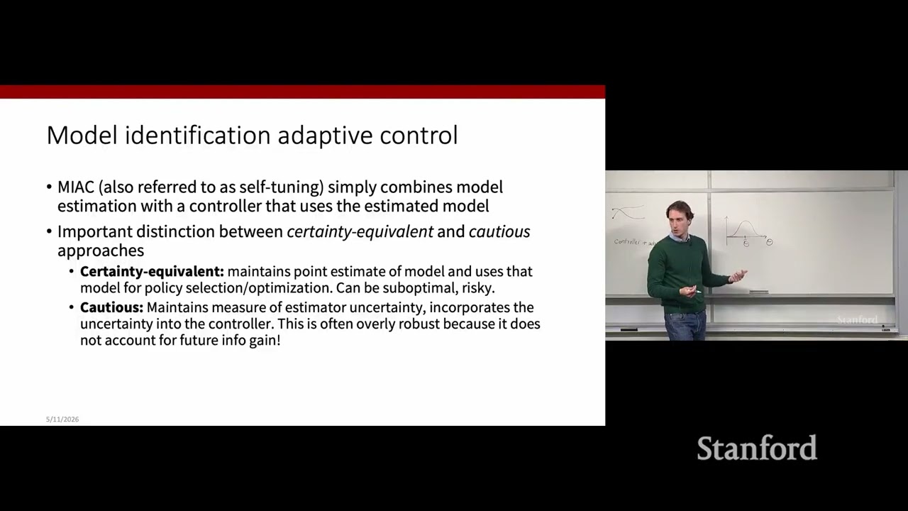
- [05:26](https://www.youtube.com/watch?v=7YdOx-ih0II&t=326s) Model Identification Adaptive Control (MIAC) decouples dynamic estimation from control execution, enabling modular pairings under certainty equivalence or cautious distributions.
- [13:08](https://www.youtube.com/watch?v=7YdOx-ih0II&t=788s) Imitation learning fits policies directly from paired demonstrations of state-action tuples, whereas reinforcement learning discovers policies through trial-and-error optimization against scalar reward signals.
- [14:36](https://www.youtube.com/watch?v=7YdOx-ih0II&t=876s) Pure imitation learning is strictly bottlenecked by demonstrator performance, prompting modern architectures to use IL for baseline behavior acquisition followed by downstream RL policy fine-tuning.
- [18:13](https://www.youtube.com/watch?v=7YdOx-ih0II&t=1093s) Supervised learning under maximum likelihood estimation forms the mathematical foundation of imitation learning, minimizing negative log-likelihood across collected state-action datasets.
- [23:17](https://www.youtube.com/watch?v=7YdOx-ih0II&t=1397s) Imitation learning branches into Behavior Cloning, which maps states directly to actions, and Inverse Reinforcement Learning, which reconstructs the expert's implicit reward function as an objective field.
- [29:01](https://www.youtube.com/watch?v=7YdOx-ih0II&t=1741s) ALVINN established the early precedent for end-to-end physical AI by mapping front-facing visual imagery directly to vehicle steering commands using artificial neural networks.
- [31:10](https://www.youtube.com/watch?v=7YdOx-ih0II&t=1870s) Closed-loop robotic execution causes compounding errors and covariate shift in behavior cloning, as the policy actively induces its own test-time state distribution.
- [35:54](https://www.youtube.com/watch?v=7YdOx-ih0II&t=2154s) Inverse Reinforcement Learning decouples objective representations from specific trajectories, enabling robots to adapt navigation paths across changing environments without re-learning policies.
- [38:10](https://www.youtube.com/watch?v=7YdOx-ih0II&t=2290s) Reinforcement learning models closed-loop agent-environment interactions where agents select actions, observe environment transitions, and receive scalar performance feedback.
- [45:42](https://www.youtube.com/watch?v=7YdOx-ih0II&t=2742s) RL enables the emergence of novel strategies unconstrained by human biases, exemplified by DeepMind's AlphaGo Move 37 and automated tunneling strategies in Atari Breakout.
- [49:14](https://www.youtube.com/watch?v=7YdOx-ih0II&t=2954s) In quadrupedal locomotion, RL acts as a physics distillation engine, embedding complex simulated contact dynamics into fast, deployable neural network policies.
- [53:10](https://www.youtube.com/watch?v=7YdOx-ih0II&t=3190s) Markov Decision Processes formalize reinforcement learning tasks, defining trajectory distributions and maximizing expected cumulative discounted rewards parameterized by discount factor gamma.
- [59:26](https://www.youtube.com/watch?v=7YdOx-ih0II&t=3566s) The action-value function Q(x, u) allows model-free evaluation and policy improvement by scoring alternate candidate actions without requiring an explicit transition dynamics model.
- [01:05:43](https://www.youtube.com/watch?v=7YdOx-ih0II&t=3943s) RL taxonomy divides into model-free methods (split into policy optimization and value-based approaches) and model-based approaches leveraging known or learned physical dynamics.
- [01:07:32](https://www.youtube.com/watch?v=7YdOx-ih0II&t=4052s) Direct policy parameterization is often practically simpler than modeling full underlying physics, as seen in cartpole balancing and everyday human thermal feedback adjustments.
- [01:11:17](https://www.youtube.com/watch?v=7YdOx-ih0II&t=4277s) Frontier autonomy models like NVIDIA's Alpamayo-R1 unify pre-training, supervised demonstration fine-tuning, and reinforcement learning alignment into a single multi-tier architecture.
## Detailed walkthrough
### [00:05](https://www.youtube.com/watch?v=7YdOx-ih0II&t=5s) Recap: Classical Learning-Based Control, System ID, and MRAC
The lecture opens with an "extreme recap" of the previous session to establish continuity before moving into modern paradigms. The foundational motivation for learning-based control is the need to relax the classical assumption that the system dynamics are known perfectly. In practical robotics and aerospace settings, engineers frequently face unknown dynamics or physical parameters that must be estimated from data. On Monday, the class explored classical approaches to this challenge, beginning with System Identification (sys ID). In sys ID, the practitioner collects rollouts or trajectories reflecting the system's evolution, frames the task as a regression problem (such as linear regression), and fits an approximate model of the dynamics.
Dr. Gammelli then revisits Model Reference Adaptive Control (MRAC), a direct adaptive control method where the controller, an adaptive parameter-adjustment mechanism, and the physical plant operate as a coupled system. Rather than fitting dynamics as an isolated offline task, adaptive control analyzes this interconnected system directly, leaning on Lyapunov stability theory to guarantee stability. In MRAC, the adaptive component specifically tunes the control law online to force the plant to track a prescribed reference signal.
```mermaid
flowchart LR
accTitle: Classical Learning-Based Control Paradigms
accDescr: Diagram contrasting System Identification with Model Reference Adaptive Control.
subgraph SysID["System Identification (Sys ID)"]
A["Collect Rollouts / Trajectories"] --> B["Regression Problem"]
B --> C["Approximate Model of Dynamics"]
end
subgraph MRAC["Model Reference Adaptive Control (MRAC)"]
D["Reference Signal"] --> E["Adaptive Controller"]
E --> F["Coupled Plant Dynamics"]
F -.->|"Lyapunov Stability Analysis"| E
end
```
[02:47](https://www.youtube.com/watch?v=7YdOx-ih0II&t=167s) Reference Signals, Identifiability, and Persistent Excitation in MRAC
Reflecting on the MRAC examples covered previously, Dr. Gammelli clarifies that those derivations were somewhat "contrived" from an analytical perspective. In class, the control law $u$, the candidate Lyapunov function $V$, and the parameter adaptation law were essentially handed to the students from the outside so they could focus purely on the mechanics of stability analysis. In real engineering practice, the designer must synthesize all three components themselves before conducting the Lyapunov analysis.
The discussion then turns to the nature of the reference signal itself, uncovering a fundamental tension between tracking and parameter estimation:
- **Trivial Reference Signals and Identifiability:** If the reference signal is simple—such as zero or a constant value—multiple distinct parameter values can yield zero tracking error. Because MRAC is fundamentally driven to minimize tracking error rather than estimation error, it suffers from an identifiability problem: it achieves its tracking objective without ever recovering the true physical parameters.
- **Complex Reference Signals and Persistent Excitation:** If the reference signal is sufficiently rich and complex, accurate tracking cannot occur unless the estimated parameters match the true values. This forces the system back into the domain of *persistent excitation*: the plant must be probed with rich, varied inputs to guarantee that parameter estimates converge to their ground truth.
[05:26](https://www.youtube.com/watch?v=7YdOx-ih0II&t=326s) Model Identification Adaptive Control (MIAC) vs. MRAC
The lecture completes its review of classical methods by introducing Model Identification Adaptive Control (MIAC), an indirect adaptive control architecture. Unlike direct methods, MIAC embeds system identification into an inner loop: it continuously estimates a model of the dynamics and immediately feeds that estimated model into a controller that treats the parameters as if they were ground truth. Because the identification module and the control algorithm are decoupled, MIAC is modular and customizable, allowing designers to pair arbitrary system identification schemes with arbitrary controllers.
Dr. Gammelli distinguishes between two core philosophies for handling parameter uncertainty within MIAC:
- **Certainty Equivalence:** The estimator provides a single point estimate $\hat{\theta}$, which the controller trusts entirely without accounting for estimation error.
- **Cautious Approach:** The estimator maintains a probability distribution over the unknown parameters $\theta$. This distribution explicitly captures the system's epistemic uncertainty, allowing the controller to act cautiously in regions where data is sparse.
| Feature | Model Reference Adaptive Control (MRAC) | Model Identification Adaptive Control (MIAC) |
|:--- |:--- |:--- |
| **Primary Objective** | Directly minimizes tracking error against a reference signal | Minimizes data-fitting error (parameter estimation) |
| **Architecture** | Direct: tightly coupled adaptation and control | Indirect: modular inner-loop sys ID driving a separate controller |
| **Stability Guarantees** | Strong: stability and convergence are built-in via Lyapunov design | Weaker: difficult to guarantee due to dependence on parameter accuracy |
| **Flexibility** | Rigidly constrained by the analytical Lyapunov synthesis | Highly flexible: arbitrary models and controllers can be coupled |
[08:50](https://www.youtube.com/watch?v=7YdOx-ih0II&t=530s) The Modern Paradigm: Imitation Learning and Reinforcement Learning
With classical adaptive control concluded, Dr. Gammelli transitions to the main subject of the lecture: Imitation Learning (IL) and Reinforcement Learning (RL). On the course roadmap, this marks a shift from the top-left quadrant (classical learning-based control) to the top-right quadrant (modern learning-based and end-to-end approaches)—representing what Dr. Gammelli characterizes as "probably one of the most active areas of research right now when looking at control and autonomous systems."
This surge of interest is fueled by the deployment of foundation models, Large Language Models (LLMs), and Vision-Language Models (VLMs) directly in closed-loop control pipelines. While high-level hype surrounds these multimodal architectures, Dr. Gammelli stresses that virtually all end-to-end robotic systems developed over the past three to four years rely on imitation learning or reinforcement learning as their underlying learning signals.
Key real-world applications driving this shift include:
- **Robotic Manipulation:** End-to-end vision-to-action networks trained on expert demonstrations via imitation learning.
- **Autonomous Driving:** Industrial stacks, such as NVIDIA's Alpamayo AV stack, combining supervised imitation learning from human driving data with reinforcement learning for fine-grained policy optimization.
- **Foundation Model Alignment:** Large language and multimodal models fine-tuned via RL (such as RLHF) to turn raw next-token predictors into aligned, helpful, and safe interactive agents.
Dr. Gammelli sets up the overarching question for the remainder of the lecture: how do these modern, data-driven frameworks interface with the formal optimal control formulations developed throughout the course?
[11:38](https://www.youtube.com/watch?v=7YdOx-ih0II&t=698s) From Model-Based Optimal Control to Learning-Based Approaches
Every method examined in the course up to this point has shared a single underlying objective: establishing a concrete mechanism to transition from a state representation—whether more or less structured—to the specification of an optimal control input. This transition represents the "gold standard" pursued across classical optimal control. Prior lectures operated entirely within an initial framework categorized as "option one." Under option one, an engineer must first acquire a deep, principled understanding of the physical problem setting, typically formalized as explicit differential or difference equations governing the system dynamics. Using this analytical model, one then designs an optimization routine. The canonical extreme of this approach is indirect methods, where an intimate mathematical understanding of the system dynamics is leveraged via the calculus of variations to derive necessary optimality conditions (such as Pontryagin's Minimum Principle) and solve boundary value problems.
The course now pivots away from purely model-based derivations toward data-driven learning paradigms, categorized on the slides as options two and three. Rather than manually engineering controllers from dynamic equations, the task of translating state observations into control actions is directly cast as a machine learning problem.
```mermaid
flowchart TD
accTitle: Control paradigms comparison
accDescr: Diagram contrasting model-based optimal control with learning-based imitation and reinforcement learning.
subgraph Option1["Option 1: Model-Based Control"]
A["Deep System Understanding<br/>(Equations of Motion)"] --> B["Analytical Derivation<br/>(Optimality Conditions)"]
B --> C["Optimal Control Input"]
end
subgraph LearningOptions["Learning-Based Formulations"]
subgraph Option2["Option 2: Imitation Learning"]
D["Demonstration Dataset<br/>(State-Action Tuples)"] --> E["Supervised Approximation<br/>(Mimic Teacher)"]
end
subgraph Option3["Option 3: Reinforcement Learning"]
F["Environment Interaction<br/>(Trial and Error)"] --> G["Reward Metric Optimization<br/>(Find Best Strategy)"]
end
end
```
[13:08](https://www.youtube.com/watch?v=7YdOx-ih0II&t=788s) Imitation Learning vs. Reinforcement Learning: Demonstrations vs. Trial and Error
Learning to map states to actions splits into two distinct philosophical frameworks: imitation learning and reinforcement learning. Imitation learning is succinctly characterized by the phrase "learn from demonstrations." In this paradigm, practitioners collect datasets of prior experience structured as tuples containing observed states and the corresponding control decisions executed within those states. The learning algorithm's goal is to estimate and approximate the functional mapping between them. Crucially, imitation learning relies on the presence of an expert or teacher whose logged decisions are assumed to demonstrate good, desirable behavior.
Reinforcement learning (RL), conversely, operates on the principle of learning through trial and error. Rather than pairing a state with an expert demonstration of what to do, the algorithm observes the state it occupies and receives a scalar score or evaluation metric indicating how favorable a particular chosen action was. Dr. Gammelli highlights the core philosophical contrast between the two paradigms:
- **Imitation Learning:** Relies on an explicit teacher or supervisor prescribing what action *should* be taken in any given state.
- **Reinforcement Learning:** Lacks any supervisory agent showing the correct trajectory; instead, the agent receives an evaluative performance signal and must actively explore alternative strategies to discover which behavior yields the highest cumulative reward in practice.
[14:36](https://www.youtube.com/watch?v=7YdOx-ih0II&t=876s) Student Q&A: Teacher Bottlenecks and Multi-Stage Training Pipelines
A student raises an essential question regarding dataset quality: is the training data fed into an imitation learning algorithm treated as an incontrovertible, perfect ground-truth model, or exists there a mechanism to communicate that a demonstration is merely "good" but open to improvement? Dr. Gammelli emphasizes that this hits directly on the fundamental limitation of imitation learning. At face value, standard imitation learning assumes that the empirical mapping being fitted constitutes optimal behavior; consequently, the resulting policy is fundamentally bounded and "bottlenecked by the performance of your teacher." While an asterisk belongs on that claim—since specialized algorithmic variations can re-weight or prioritize higher-performing trajectories over lower-performing ones—the baseline paradigm cannot surpass the capability of the demonstrations provided.
A follow-up question asks whether autonomous systems practicalize this by using machine learning to absorb basic behaviors first before switching to reinforcement learning for fine-tuning once task constraints are understood. Dr. Gammelli confirms that modern autonomy stacks rely heavily on layered, multi-stage training pipelines:
- **Inspiration from NLP and LLMs:** Autonomous vehicle and robotic training regimes have largely adopted paradigms popularized by large language models, where training is partitioned into distinct progressive stages.
- **Pre-training Phase:** Broad, large-scale supervised learning or imitation learning is utilized on massive datasets to absorb general environmental rules, dynamic priors, and baseline competence.
- **Fine-tuning via RL:** After establishing a strong initialization through imitation, reinforcement learning is applied downstream to optimize performance, explore alternative actions, and tune policies beyond the teacher's original ceiling.
[16:54](https://www.youtube.com/watch?v=7YdOx-ih0II&t=1014s) Course Roadmap and Foundational References
Setting up the technical agenda, Dr. Gammelli outlines the roadmap: the lecture begins with a rapid grounding in notation and supervised learning foundations, then establishes a unified conceptual mental model comparing imitation learning and reinforcement learning, unpacking their shared mathematical structures and practical trade-offs. Detailed, concrete algorithmic implementations for both paradigms will follow across subsequent lectures.
For students looking to dive deeper, Gammelli points to key foundational literature and courses:
- **Class Textbook:** *Principles of Robot Autonomy* (Pavone et al.).
- **Canonical RL Reference:** Richard S. Sutton and Andrew G. Barto's *Reinforcement Learning: An Introduction*.
- **University Courses:** Stanford's Deep Reinforcement Learning course (CS234) and UC Berkeley's counterpart curriculum (CS285).
[18:13](https://www.youtube.com/watch?v=7YdOx-ih0II&t=1093s) Supervised Learning Foundations: Mapping Inputs to Outputs via Likelihood Maximization
Supervised learning provides the structural foundation for imitation learning. At its core, supervised learning seeks to uncover a parameterized mapping $f_\theta$ linking an input space $\mathcal{X}$ to an output space $\mathcal{Y}$. This standard formulation subsumes classic regression and classification problems. In vision classification, for instance, the input $x$ is an RGB image array of a scene or animal, and the output $y$ is a discrete category label denoting the detected object. More broadly, the framework operates over arbitrary feature vectors $x \in \mathcal{X}$ and target vectors $y \in \mathcal{Y}$ provided as paired observations $(x_i, y_i)$.
Dr. Gammelli illustrates the regression setting with an intuitive example: given scattered data points $(x_i, y_i)$ in two dimensions (visualized as red dots), one might fit a parametric parabolic curve $f(x; \theta)$ parameterized by weights $\theta$. From a deterministic perspective, parameter estimation minimizes an empirical discrepancy metric, such as a sum of squared errors:
Equivalently, the task can be framed probabilistically through maximum likelihood estimation (MLE). Under this perspective, one posits that targets $y$ are distributed according to a conditional probability density centered at the function's output:
Pictorially, this corresponds to placing a small Gaussian distribution over every evaluated prediction point. Fitting the dataset translates to maximizing the joint likelihood across all independent training observations:
Because taking the product of many probability densities between 0 and 1 causes severe numerical underflow and creates an exceptionally sharp, ill-behaved optimization surface, standard practice applies a monotonic logarithmic transformation. Taking the logarithm preserves the precise locations of the extrema while converting the product into a sum. To match standard optimization conventions, the problem is converted into minimizing the negative log-likelihood (NLL):
This transformation smooths out the objective landscape into a well-behaved optimization problem while retaining the identical optimal estimator $\hat{\mu}$. This supervised learning apparatus serves as the exact statistical bedrock onto which imitation learning policies are grafted.
[23:17](https://www.youtube.com/watch?v=7YdOx-ih0II&t=1397s) Foundations of Imitation Learning: Transferring Skills from Experts
Imitation learning fundamentally represents a class of techniques designed to transfer skills directly from an expert to a learner. In robotics, the "expert" is typically either an experienced human operator or a pre-existing control policy, while the "learner" is the target policy being approximated. To illustrate this setup, Dr. Daniele Gammelli describes a bimanual manipulation system operated by a human teleoperator. As the human acts, the system logs their control inputs, treating the human teleoperator as the skilled teacher. The core computational challenge is then formalizing a mapping from the physical states of the bimanual manipulator to the corresponding control actions, typically by minimizing an error metric relative to what the human expert would have chosen in those exact states.
```mermaid
flowchart LR
accTitle: Overview of Imitation Learning Paradigms
accDescr: Diagram showing how expert demonstrations feed into either Behavior Cloning or Inverse Reinforcement Learning.
subgraph DataCollection["Data Collection"]
E["Expert Demonstrator<br>(Human or Controller)"] --> D["Demonstration Dataset<br>Pairs (x, u)"]
end
subgraph Approaches["Imitation Paradigms"]
D --> BC["Behavior Cloning (BC)<br>Direct Mapping: States -> Controls"]
D --> IRL["Inverse Reinforcement Learning (IRL)<br>Infer Reward: r(x, u)"]
IRL --> OPT["Policy Optimization<br>(Derive Policy pi)"]
end
```
At a higher theoretical level, imitation learning assumes access to an offline dataset of state-control pairs $(x, u)$ gathered by observing the expert acting in the physical world. Under the broad umbrella of imitation learning, algorithms fall into two distinct and complementary paradigms:
- **Behavior Cloning (BC):** The most direct and intuitive method, which frames policy acquisition as learning a parametric function $\pi(x)$ that directly maps state $x$ to control $u$, minimizing prediction errors on recorded pairs.
- **Inverse Reinforcement Learning (IRL) / Inverse Optimal Control:** Rather than directly predicting actions, IRL infers the underlying reward function or objective metric $r(x, u)$ that the expert was implicitly optimizing.
---
[26:35](https://www.youtube.com/watch?v=7YdOx-ih0II&t=1595s) Behavior Cloning vs. Inverse Reinforcement Learning in Practice
Addressing a student question about extracting the underlying "intent" or thinking process, Dr. Gammelli contrasts how each paradigm handles a concrete spatial navigation task with a fixed start and goal location. In behavior cloning, the dataset consists of successful trajectory rollouts navigating between these points, and the agent learns to reproduce those exact paths. In inverse reinforcement learning, the algorithm instead reconstructs the underlying cost or reward landscape—such as a vector field where the cost is minimal at the target state and rises across surrounding states.
A student observes that under IRL, finding controls still requires an explicit downstream optimization step. Dr. Gammelli confirms this: IRL does not yield an actionable control rule by itself; it extracts an analytical objective that must then be solved using standard trajectory optimization or optimal control solvers. Autonomous driving illustrates why this extra step is valuable. Formally writing down an analytical mathematical formula for "good driving" is notoriously difficult and highly subjective. However, gathering raw human driving logs is cheap and scalable. IRL reverse-engineers the implicit utility function governing human drivers from those logs, allowing formal control methods to optimize against that recovered objective.
---
[29:01](https://www.youtube.com/watch?v=7YdOx-ih0II&t=1741s) Early Behavior Cloning: The ALVINN Milestone
Behavior cloning simplifies policy synthesis into a pure supervised learning formulation. The canonical workflow takes expert teleoperation demonstrations and fits a policy $\pi_\theta(x)$ using standard supervised regression, classification, or maximum likelihood estimation.
Historically, this approach achieved a breakthrough in the late 1980s through research at Carnegie Mellon University (CMU) involving an autonomous military vehicle (ALVINN). The system processed front-facing camera imagery directly through a small artificial neural network that predicted the vehicle's steering angle. Although restricted to simple roads and controlled environments, the architecture was groundbreaking: it established the prevailing template of modern physical AI systems, learning an end-to-end mapping directly from high-dimensional visual inputs to low-level actuator commands.
---
[31:10](https://www.youtube.com/watch?v=7YdOx-ih0II&t=1870s) The Core Pitfalls: Compounding Errors and Covariate Shift
Despite its elegance, the standard behavior cloning recipe is not guaranteed to work reliably on physical systems. Imitation learning diverges fundamentally from classical supervised learning due to the closed-loop nature of embodied autonomy:
1. **Compounding Execution Errors:** In standard supervised learning, test samples are drawn independently. In closed-loop robotics, any slight policy error $\hat{u}_0 \neq u_0$ steers the robot to an altered state $\hat{x}_1$. This new state often lies outside the support of the expert training distribution, which generates even worse downstream control predictions. This feedback loop degrades performance exponentially over time:
$$\text{Distribution Shift: } x_0 \xrightarrow{\hat{u}_0} \hat{x}_1 \notin \text{supp}(P_{\text{expert}}) \implies \text{Compounding Divergence}$$
2. **Active State Distribution Induction:** Because autonomous agents are active participants in their environment, their own real-time mistakes dictate the exact distribution of states they observe next—a dynamic entirely absent in passive classification tasks.
3. **Physical Constraints and Kinematics:** Unlike open-vocabulary image classifiers that can output any semantic token, physical systems must obey actuator limits, non-holonomic kinematics, and joint limits.
4. **Embodiment Gaps:** Demonstrations often originate from different physical forms, such as attempting to teach a humanoid robot control policies using human video recordings.
5. **Covariate Shift:** The state visitation distribution induced by executing the learned policy systematically diverges from the state distribution induced by the demonstrator.
6. **Data Collection Costs:** Collecting rich robotic demonstrations through continuous teleoperation or real-world vehicle logging is orders of magnitude more expensive and hazardous than scraping unlabeled images or web text.
[035:54] Inverse Reinforcement Learning and Generalizable Objectives
Before moving into the formal foundations of reinforcement learning, Dr. Gammelli pauses for questions and then addresses inverse reinforcement learning (IRL) as an orthogonal paradigm to standard imitation learning. Rather than directly mapping states to actions via behavioral cloning, inverse reinforcement learning aims to recover the underlying reward function from an expert's demonstrations.
To ground this intuition, he offers a concrete warehouse robotics example: suppose a mobile robot must navigate from a starting point $A$ to a goal point $B$. Under behavioral cloning, one collects demonstrations traversing from $A$ to $B$ and trains a policy to imitate those exact controls. That policy will perform reliably in identical setups, but if the warehouse layout is rearranged, the cloned policy quickly meets its limits because it memorized paths rather than underlying objectives. By contrast, if the algorithm infers the expert’s implicit objective—for instance, a reward structure where moving closer to the goal yields positive reward and approaching obstacles yields negative reward—it acquires a generalizable representation. Dr. Gammelli describes this recovered reward as acting like a "vector field in the space of possible paths." While IRL is not unconditionally superior to behavioral cloning, it fundamentally decouples the learning of the objective from the execution of the policy, enabling adaptation across varying configurations.
[038:10] The Reinforcement Learning Formalism and Interaction Loop
Dr. Gammelli formally introduces reinforcement learning as a mathematical framework for learning-based decision making through experience, operating via trial and error. The framework is grounded in a closed-loop interaction between two primary entities: the agent (the decision-maker or policy) and the environment (the world or dynamical system).
```mermaid
flowchart LR
accTitle: Reinforcement Learning Interaction Loop
accDescr: Diagram showing the cyclic interaction where the agent emits actions to the environment and receives updated states and scalar rewards.
subgraph AgentSystem["Policy / Decision Maker"]
Agent["Agent (Policy π)"]
end
subgraph WorldSystem["Dynamical System"]
Env["Environment"]
end
Agent -->|"Action / Control (u_t)"| Env
Env -->|"Next State (x_{t+1}) & Reward (r_t)"| Agent
```
The interaction proceeds sequentially over time:
1. At step $t$, the agent observes the current system state $x_t$.
2. The agent executes an action (or control input) $u_t$.
3. The environment consumes the action and transitions to an updated state $x_{t+1}$, returning a scalar performance metric known as the reward $r_t$.
4. Unrolling this interaction over time generates a trajectory $\tau = (x_0, u_0, r_0, x_1, u_1, r_1, \dots)$.
Every reinforcement learning algorithm fundamentally leverages these sampled trajectories to improve the policy, refining behavior based on performance feedback rather than external supervision.
[040:25] Core Terminology: Policies, Rewards, Value Functions, and Models
Establishing standard terminology from the computer science and machine learning literature, Dr. Gammelli contrasts standard control assumptions with RL definitions:
- **Policy ($\pi$):** While classical optimal control typically assumes a deterministic mapping $u = \pi(x)$, RL predominantly treats the policy as a conditional probability distribution over actions given states, $\pi(u \mid x)$. In a discrete navigation task like Gridworld, the policy outputs a probability distribution over the four cardinal directions; in continuous control domains, it is often modeled as a parametric continuous distribution, such as a Gaussian distribution over candidate actions.
- **Environment:** Represented mathematically as a conditional state-transition distribution $p(x_{t+1} \mid x_t, u_t)$.
- **Reward ($r_t$):** A scalar function evaluating immediate, single-step success for taking a specific control $u_t$ in a state $x_t$.
- **Value Function ($V^\pi$ or $Q^\pi$):** Unlike the immediate reward, the value function captures expected cumulative performance over the long run. Because both the policy and the underlying system transitions may be stochastic, an action taken at state $x_t$ fans out into a wide tree of possible future trajectories. The value function computes the expected value of future rewards under policy $\pi$. Dr. Gammelli emphasizes that estimating value functions is the true "golden standard" in reinforcement learning, because agents ultimately aim to maximize overall task success rather than instantaneous feedback.
- **Models (Model-Free vs. Model-Based RL):** An internal model represents the agent's approximate understanding of the environment's transition dynamics, $\hat{p}(x_{t+1} \mid x_t, u_t)$. Whether an algorithm constructs and leverages such a predictive model or bypasses dynamics modeling entirely dictates the split between **model-based** and **model-free** reinforcement learning.
[045:42] Why Reinforcement Learning: Emergent Strategies and Complex Tasks
Dr. Gammelli turns to why one would choose reinforcement learning over alternative techniques. Its most compelling capability is its ability to discover novel, unexpected solutions. Unlike imitation learning, where performance is fundamentally bounded by the competence of the demonstrator, RL has "no teacher." Agents are free to explore strategies purely guided by reward maximization.
He cites two landmark milestones in modern artificial intelligence to illustrate this trait:
- **Atari Breakout (mid-2010s):** Early deep RL agents began by flailing blindly, but through trial and error learned proficient paddle control. Eventually, the agent discovered an optimal, counter-intuitive strategy: repeatedly digging a tunnel along the side of the wall to trap the ball behind the bricks, racking up massive points automatically without manual human prompting.
- **AlphaGo vs. Lee Sedol (2016):** In game two of the famous tournament, DeepMind's AlphaGo played the legendary "Move 37." Commentators and top Go professionals initially viewed the placement as a bizarre blunder, but it proved to be a game-winning move that permanently altered how human masters analyzed the game.
Beyond finding creative solutions, reinforcement learning excels at directly optimizing complex, non-linear reward functions in high-dimensional domains where analytical controllers struggle, such as quadrupedal robot locomotion traversing rough, unstructured terrain.
[49:14](https://www.youtube.com/watch?v=7YdOx-ih0II&t=2954s) Reinforcement Learning in Robot Locomotion and Physics Distillation
While analytical and optimization-based control tools have long dominated robotics, reinforcement learning has rapidly emerged as the "de facto standard for basically robot locomotion." This paradigm shift is driven by the rise of highly parallelizable simulation environments, which allow robots to master complex navigation and locomotion strategies through millions of simulated interactions. Instead of relying on rigid, hand-crafted analytical assumptions regarding complex contact dynamics or attempting to explicitly identify intricate system models, practitioners let agents explore freely and discover robust behaviors directly.
In response to a student question about whether contact dynamics are still being modeled inside the simulator, Dr. Gammelli clarifies the nature of this simulation-to-policy pipeline. The simulator itself relies on a high-fidelity, physics-based engine that accurately captures physical interactions; however, evaluating these complex physics equations directly in real time can be prohibitively expensive. Reinforcement learning serves as a mechanism to "distill this physics knowledge into a policy." The resulting policy is simply a neural network mapping state inputs to control outputs. Although the policy does not explicitly perform physics calculations during deployment, it has implicitly internalized the underlying physical constraints and contact behaviors during training.
```mermaid
flowchart LR
accTitle: Physics Distillation via Reinforcement Learning
accDescr: High-fidelity physics simulation is distilled into a lightweight neural network policy through parallel interaction.
subgraph SimEngine["Simulation Environment"]
A["Accurate Physics & Contact Dynamics"] --> B["Highly Parallel Simulator"]
end
subgraph Learning["Policy Distillation"]
B --> C["Trial-and-Error Experience"]
C --> D["Neural Network Policy π(u|x)"]
end
subgraph Deployment["Real-World Execution"]
D --> E["Fast Input-to-Output Mapping"]
end
```
---
[50:46](https://www.youtube.com/watch?v=7YdOx-ih0II&t=3046s) How Reinforcement Learning Differs from Standard Machine Learning
Reinforcement learning diverges sharply from standard supervised machine learning paradigms across several foundational dimensions:
First, RL entirely lacks explicit supervision signals. There is no external supervisor providing target ground-truth actions; the agent only observes a scalar reward function. The feedback does not demonstrate what the optimal choice should have been, but merely assesses how good or bad the chosen action turned out to be.
Second, RL systems constantly face the issue of delayed feedback. Dr. Gammelli illustrates this with the game of chess: it is exceptionally difficult to determine the value of a specific opening or mid-game move in isolation, because the only definitive feedback arrives at the very end of the match when the agent either wins or loses. This gap gives rise to the classic "credit assignment" problem—the challenge of deciphering which earlier actions were actually responsible for late-stage outcomes. Modern RL methods address this through value functions and related mechanisms.
Finally, RL fundamentally violates the independent and identically distributed (I.I.D.) data assumption, which stands as "one of the most fundamental assumptions in statistical learning theory." In reinforcement learning, every action an agent executes alters the environment and dictates the future states it will encounter. Because subsequent observations are intrinsically coupled to policy decisions, the data stream is non-independent, making the learning dynamics notoriously prone to instability. Most RL algorithms incorporate specialized regularization techniques to manage this divergence.
---
[53:10](https://www.youtube.com/watch?v=7YdOx-ih0II&t=3190s) The Markov Decision Process Formalism and Objective
Reinforcement learning is formally framed using the mathematical structure of a Markov Decision Process (MDP). Dr. Gammelli advises students to develop "plasticity in dealing with different notation," as conventions differ across academic communities:
The probability of an entire trajectory $\tau = (x_0, u_0, x_1, u_1, \dots)$ is governed by conditional independence properties, factoring into the initial state distribution and two distinct sources of system stochasticity—the environment transition dynamics and the stochastic policy:
The scalar discount factor $\gamma$ serves a dual role: intuitively, it tunes how much the agent prioritizes immediate feedback relative to long-term returns; mathematically, it guarantees convergence in infinite-horizon settings by keeping the infinite sum bounded and tractable.
---
[57:40](https://www.youtube.com/watch?v=7YdOx-ih0II&t=3460s) Formulating Real-World Tasks as MDPs: Chess and Quadruped Locomotion
Before executing any learning algorithm, the practitioner must clearly cast the physical problem into the formal tuple of an MDP. Dr. Gammelli contrasts two concrete examples:
- **Chess:**
- *State Space ($\mathcal{X}$):* The complete configuration of remaining pieces across the 64 squares of the board.
- *Action Space ($\mathcal{U}$):* The set of all legal moves available given the current board arrangement.
- *Dynamics ($p(x_{t+1} \mid x_t, u_t)$):* Deterministic transitions, where selecting a move leads directly to the resulting piece placement.
- *Reward Function ($r$):* Sparse terminal feedback, such as $+1$ for a win, $-1$ for a loss, and $0$ for non-terminal moves.
- **Quadruped Locomotion:**
- *State Space ($\mathcal{X}$):* The full kinematic pose, base orientation, linear and angular velocities, and joint angles of the quadruped.
- *Action Space ($\mathcal{U}$):* Actuation commands, typically parameterized as joint torque setpoints for each leg motor.
- *Dynamics ($p(x_{t+1} \mid x_t, u_t)$):* Physical evolution governed by contact dynamics, ground friction, and inertial effects.
- *Reward Function ($r$):* Continuous shaping terms that award positive values for forward velocity, penalize falling or joint limit violations, and assign neutral values for balanced stance.
---
[59:26](https://www.youtube.com/watch?v=7YdOx-ih0II&t=3566s) Foundations of Value Functions: State Value V(x) vs Action-Value Q(x, u)
Value functions serve as the algorithmic backbone for addressing credit assignment in reinforcement learning. Because value reflects anticipated future returns, any value function is fundamentally conditioned on a particular behavioral policy $\pi$—it measures expected performance under the assumption that the agent continues to act according to that specific policy.
```mermaid
flowchart TD
accTitle: Comparison of V and Q Value Functions
accDescr: Decision tree illustrating the evaluation points of the state value function V(x) versus the action-state value function Q(x, u).
subgraph StateVal["State Value Function V^π(x)"]
S1["Current State x"] -->|"Sample u ~ π(·|x)"| A1["Policy Action u"]
A1 --> E1["Expected Total Return"]
end
subgraph ActionVal["Action-State Value Function Q^π(x, u)"]
S2["Current State x"] -->|"Force specific action u"| A2["Candidate Action u"]
A2 -->|"Follow π thereafter"| E2["Expected Total Return"]
end
```
The course introduces two primary formulations:
- **State Value Function ($V^\pi(x)$):** Quantifies the expected cumulative discounted reward accumulated when starting from state $x$ and selecting all subsequent actions according to policy $\pi$:
$$V^\pi(x) = \mathbb{E}_{\tau \sim p(\tau)} \left[ \sum_{t=0}^\infty \gamma^t r(x_t, u_t) \;\middle|\; x_0 = x, \; u_t \sim \pi(\cdot \mid x_t) \right]$$
- **Action-State Value Function ($Q^\pi(x, u)$):** Quantifies the expected cumulative discounted reward starting from state $x$, executing an arbitrary specific control action $u$ at the current step, and strictly adhering to policy $\pi$ thereafter:
$$Q^\pi(x, u) = \mathbb{E}_{\tau \sim p(\tau)} \left[ \sum_{t=0}^\infty \gamma^t r(x_t, u_t) \;\middle|\; x_0 = x, \; u_0 = u, \; u_t \sim \pi(\cdot \mid x_t) \text{ for } t \ge 1 \right]$$
Dr. Gammelli asks the class why $Q$-functions are generally more practical for control synthesis than $V$-functions. A student points out that $Q$-functions allow an agent to evaluate the consequence of deviating from its current policy—ranking alternate candidate actions directly without needing to query an explicit dynamics transition model. Dr. Gammelli confirms that this makes the $Q$-function especially suited for model-free policy improvement and exploration.
[01:02:09](https://www.youtube.com/watch?v=7YdOx-ih0II&t=3729s) Action Selection via Optimal Q-Functions
Following a student's observation about using value estimates to plan ahead—similar to evaluating whether moving a knight in chess leads to a winning position—Dr. Gammelli highlights the core practical utility of the optimal action-value function, $Q^*(s, a)$. Ultimately, control requires an operational mechanism for picking the immediate next action. If an agent can accurately estimate $Q^*(s, a)$, representing the expected future return under the optimal policy after executing action $a$ in state $s$, action selection simplifies to an optimization problem over actions alone:
$$\pi^*(s) = \arg\max_a Q^*(s, a)$$
To build intuition, Dr. Gammelli suggests imagining the Q-function as a simple lookup table. For any given state, the table provides the expected future reward associated with each available action. The agent iterates through candidate actions and selects whichever yields the highest expected return, bypassing the need for explicit forward trajectory simulations during execution.
Because state-value and action-value functions depend directly on the policy executing them, they induce a partial ordering: one policy is deemed superior to another if its value function is greater than or equal to the other across all states. The optimal state-value function $V^*(s)$ and optimal Q-function $Q^*(s, a)$ correspond to the policy that achieves the maximum expected reward across the state space. Dr. Gammelli emphasizes that these optimal functions represent the "golden standard" that RL algorithms endeavor to converge toward, urging students to firmly anchor these definitions in their minds as foundational building blocks for the upcoming lectures.
---
[01:05:43](https://www.youtube.com/watch?v=7YdOx-ih0II&t=3943s) Taxonomy of Reinforcement Learning: Model-Free vs. Model-Based
Reinforcement learning comprises a broad family of methods categorized primarily by whether they rely on an environmental dynamics model. Model-free methods discard the dynamics entirely, learning effective behaviors without attempting to approximate the transition probability distribution $p(s_{t+1} \mid s_t, a_t)$. Model-based methods, by contrast, either assume known physical dynamics—connecting directly to traditional optimal control frameworks covered earlier in the course—or explicitly learn an approximate dynamics model from data via system identification techniques, leveraging that model to plan or update the policy.
Within the model-free branch, algorithms split into policy optimization and value-based approaches:
- **Policy Optimization Methods:** Directly maximize the RL expected return objective by parameterizing the policy $\pi_\theta(a \mid s)$ and optimizing parameters using gradient ascent.
- **Value-Based Methods:** Optimize the objective implicitly by learning the optimal action-value function $Q^*(s, a)$, with the policy defined downstream as $\pi(s) = \arg\max_a Q(s, a)$.
```mermaid
flowchart TD
accTitle: Taxonomy of Reinforcement Learning Algorithms
accDescr: A tree diagram categorizing RL algorithms into model-free and model-based branches, further divided into policy optimization, value-based, known dynamics, and learned dynamics.
subgraph SubMF["Model-Free"]
MF --> PO["Policy Optimization<br/>(Direct objective optimization)"]
MF --> VB["Value-Based Methods<br/>(Implicit via Q-function estimation)"]
end
subgraph SubMB["Model-Based"]
MB --> KD["Known Dynamics<br/>(Classical optimal control)"]
MB --> LD["Learned Dynamics<br/>(System ID / model learning)"]
end
```
---
[01:07:32](https://www.youtube.com/watch?v=7YdOx-ih0II&t=4052s) Algorithmic Trade-Offs: Sample Efficiency, Stability, and System Modeling
Navigating the RL landscape requires balancing engineering trade-offs, chief among them sample efficiency and numerical stability. Sample efficiency measures how many physical or simulated environment interactions an agent must collect before converging to an effective policy. While high sample efficiency is desirable in theory, it often trades off against optimization stability: algorithms that reuse data aggressively (such as off-policy value-based algorithms) can suffer from unstable training dynamics.
Dr. Gammelli highlights that "wall-clock time is not the same as efficiency." In modern engineering environments where interactions can be parallelized cheaply across thousands of simulator instances, a sample-inefficient algorithm that possesses rock-solid convergence properties often reaches a usable policy faster in real-world wall-clock time than a fragile, sample-efficient method that requires delicate hyperparameter tuning. Problem formulation specifics also dictate algorithm selection:
- **Horizon & Resets:** Episodic settings that permit frequent restarts (such as resetting a chess board) accommodate different algorithms than infinite-horizon environments where the agent runs continuously without resets.
- **Action & State Spaces:** Algorithms must be chosen based on whether action and state spaces are continuous or discrete (for instance, evaluating $\arg\max_a Q(s, a)$ across continuous action spaces requires specialized actor-critic or continuous Q-learning machinery).
- **Representational Complexity:** It is often substantially easier to parameterize a direct control policy than it is to model complex underlying physical dynamics.
To illustrate representational complexity, Dr. Gammelli presents two everyday physical examples:
1. **The Cartpole Problem:** Writing down or identifying the full non-linear differential equations governing cartpole dynamics can be challenging. In contrast, the control policy is intuitive: if the pole tilts to the left, push the cart left to counterbalance it.
2. **Taking a Shower:** When adjusting a shower, humans do not compute fluid mechanics or thermodynamic heat propagation through water and air onto skin. "Simply, we feel something is hot, and we turn the knob." Directly learning the policy mapping sensation to action is vastly simpler than modeling the entire thermal system.
---
[01:11:17](https://www.youtube.com/watch?v=7YdOx-ih0II&t=4277s) Frontier Autonomy: Scaffolded Pipelines and Course Wrap-Up
In his closing synthesis, Dr. Gammelli cautions students against viewing imitation learning and reinforcement learning as isolated, mutually exclusive paradigms. Modern state-of-the-art autonomy stacks—particularly vision-language-action (VLA) models—do not pick one method over the other. Instead, frontier architectures assemble these techniques into multi-stage, scaffolded training pipelines where each paradigm addresses a specific phase of capability development.
As a prime illustration, Dr. Gammelli points to NVIDIA's Alpamayo-R1, an autonomous driving reasoning VLA model designed to output driving actions directly from multi-modal sensor inputs. Rather than attempting to train the entire system with pure RL from scratch, the system undergoes a multi-tiered pipeline:
1. **Internet-Scale Pre-Training:** Large foundation models undergo massive self-supervised and supervised pre-training across internet-scale text, video, and sensory data to learn world representations and commonsense reasoning.
2. **Supervised Fine-Tuning (SFT / Imitation Learning):** The pre-trained model is fine-tuned on expert human driving demonstrations, mapping visual inputs and trajectory targets directly to valid driving behaviors.
3. **Reinforcement Learning Alignment:** Finally, reinforcement learning is applied to align the system's reasoning and control policies with human safety preferences, societal driving norms, and edge-case robustness, effectively "squeezing out the last bit of performance."
Dr. Gammelli concludes the lecture by reiterating that these diverse machine learning and optimal control tools are complementary pieces of a unified toolkit, inviting remaining questions before adjourning until the next session on Monday.
## Notable quotes
> [08:50](https://www.youtube.com/watch?v=7YdOx-ih0II&t=530s) probably one of the most active areas of research right now when looking at control and autonomous systems. — Dr. Daniele Gammelli
> [14:36](https://www.youtube.com/watch?v=7YdOx-ih0II&t=876s) bottlenecked by the performance of your teacher. — Dr. Daniele Gammelli
> [35:54](https://www.youtube.com/watch?v=7YdOx-ih0II&t=2154s) vector field in the space of possible paths. — Dr. Daniele Gammelli
> [49:14](https://www.youtube.com/watch?v=7YdOx-ih0II&t=2954s) de facto standard for basically robot locomotion. — Dr. Daniele Gammelli
> [49:14](https://www.youtube.com/watch?v=7YdOx-ih0II&t=2954s) distill this physics knowledge into a policy. — Dr. Daniele Gammelli
> [50:46](https://www.youtube.com/watch?v=7YdOx-ih0II&t=3046s) one of the most fundamental assumptions in statistical learning theory. — Dr. Daniele Gammelli
> [53:10](https://www.youtube.com/watch?v=7YdOx-ih0II&t=3190s) plasticity in dealing with different notation, — Dr. Daniele Gammelli
> [01:02:09](https://www.youtube.com/watch?v=7YdOx-ih0II&t=3729s) golden standard — Dr. Daniele Gammelli
> [01:07:32](https://www.youtube.com/watch?v=7YdOx-ih0II&t=4052s) wall-clock time is not the same as efficiency. — Dr. Daniele Gammelli
> [01:07:32](https://www.youtube.com/watch?v=7YdOx-ih0II&t=4052s) Simply, we feel something is hot, and we turn the knob. — Dr. Daniele Gammelli
> [01:11:17](https://www.youtube.com/watch?v=7YdOx-ih0II&t=4277s) squeezing out the last bit of performance. — Dr. Daniele Gammelli
## Mentioned
Daniele Gammelli, Marco Pavone, Stanford University, Italian Institute of Artificial Intelligence (AI4I), NVIDIA, Alpamayo, Alpamayo-R1, Principles of Robot Autonomy, Richard S. Sutton, Andrew G. Barto, Reinforcement Learning: An Introduction, ALVINN, Carnegie Mellon University (CMU), DeepMind, AlphaGo, Lee Sedol, Pontryagin's Minimum Principle, Lyapunov, Model Reference Adaptive Control (MRAC), Model Identification Adaptive Control (MIAC), Behavior Cloning, Inverse Reinforcement Learning (IRL), Markov Decision Process (MDP)
## Video description
Lecture 14 — Intro to Imitation Learning and Reinforcement Learning
Read the companion textbook, Principles of Robot Autonomy, free online: https://porabook.com
To learn more about enrolling in AA203 Optimal and Learning-Based Control, visit: https://online.stanford.edu/courses/aa203-optimal-and-learning-based-control
Follow along with the course schedule and syllabus: https://stanfordasl.github.io/aa203/sp2526/
Bio: Dr. Daniele Gammelli is the Research Director of the Machine Intelligence for Robot Autonomy Laboratory at the Italian Institute of Artificial Intelligence (AI4I), and a Researcher in the Department of Aeronautics and Astronautics at Stanford University. Since 2022, he has been a Research Fellow at the Center for Aerospace Autonomy Research (CAESAR) at Stanford and, until 2025, at the Center for Automotive Research at Stanford (CARS). He received his Ph.D. in Machine Learning and Mathematical Optimization from the Technical University of Denmark (DTU) in 2022, where his doctoral thesis was nominated for the DTU Best Thesis of the Year Award and the DTU Young Researcher Award. Dr. Gammelli’s research focuses on developing the algorithmic foundations and system-level methodologies that enable AI-powered autonomous systems to operate safely, efficiently, and reliably in high-stakes environments, with an emphasis on aerospace autonomy and next-generation mobility systems.
Instructors:
Prof. Marco Pavone, Associate Professor of Aeronautics and Astronautics, Director of Autonomous Vehicle Research at NVIDIA
Dr. Daniele Gammelli, Research Director at the Italian Institute of Artificial Intelligence (AI4I), Researcher at the Department of Aeronautics and Astronautics, Stanford University
Full playlist: https://www.youtube.com/playlist?list=PLa9dmHsLK9dg
Dr. Daniele Gammelli contrasts classical, model-based control with modern data-driven paradigms, showing how imitation learning and reinforcement learning relax the need for known system dynamics. Rather than operating as mutually exclusive methods, modern autonomy frameworks combine these paradigms into scaffolded pipelines that pair large-scale demonstration pre-training with downstream reinforcement learning fine-tuning.
From Model-Based Control to Data-Driven Policies (11:38)
Classical optimal control relies on explicit analytical models—such as differential equations solved via indirect calculus of variations—or system identification paired with adaptive control schemes like Model Reference Adaptive Control (MRAC) and Model Identification Adaptive Control (MIAC). Dr. Gammelli explains that while these methods offer formal stability guarantees via Lyapunov theory, they demand explicit dynamics models, hand-crafted adaptation rules, or persistent excitation to ensure parameter convergence.
Modern autonomy increasingly pivots toward machine learning formulations that map state observations directly to control inputs without explicit physical modeling. This transition bifurcates into two data-driven options: imitation learning, which fits mappings from curated teacher demonstrations, and reinforcement learning, which optimizes behaviors through unguided trial-and-error environment interaction.
Imitation Learning Mechanics and Distributional Failure Modes (23:17)
Imitation learning fits parameterized policies to offline datasets of state-action tuples using supervised learning methods, often framed as negative log-likelihood minimization under Gaussian assumptions. The paradigm divides into behavior cloning, which directly learns a policy function mapping states to controls, and inverse reinforcement learning (IRL), which infers the implicit cost or reward function underlying expert behavior. While IRL requires an additional downstream optimization step to generate actionable controls, it decouples the task objective from policy execution, allowing systems to adapt when physical configurations change.
Behavior cloning, introduced historically in systems like Carnegie Mellon University's late-1980s ALVINN vehicle, faces fundamental limitations in closed-loop physical settings. Standard policies remain bounded by teacher competence. More critically, closed-loop execution violates the independent and identically distributed assumption of classical supervised learning: small control errors steer agents into unfamiliar states, inducing covariate shift and compounding execution errors that degrade performance exponentially over time.
Reinforcement Learning Formalism and Credit Assignment
Reinforcement learning removes the supervisory bottleneck of imitation learning by allowing agents to discover strategies through evaluative scalar rewards rather than correct action labels. The problem is formally cast as a Markov Decision Process (MDP) defined by states, actions, transition dynamics, and rewards. The optimization objective seeks a policy that maximizes expected cumulative discounted returns, where a discount factor balances immediate versus future rewards while guaranteeing convergence across infinite horizons.
Because external rewards are frequently delayed—exemplified by terminal win-or-loss outcomes in chess—reinforcement learning relies on value functions to resolve the credit assignment problem. While the state-value function evaluates expected returns from a given state under a specific policy, the action-value function directly evaluates candidate actions. Estimating the optimal action-value function allows an agent to select controls without needing an explicit transition dynamics model.
Algorithmic Trade-Offs and Scaffolded Autonomy Pipelines (67:32)
Selecting between model-free and model-based reinforcement learning involves balancing sample efficiency against numerical stability and representational complexity. Dr. Gammelli emphasizes that wall-clock time does not equal sample efficiency: in settings where simulation can be parallelized cheaply, sample-inefficient algorithms with stable convergence often train faster than delicate, sample-efficient alternatives. In quadrupedal robot locomotion, RL effectively distills complex contact physics from high-fidelity simulators into lightweight neural network policies that execute rapidly during deployment.
State-of-the-art autonomy stacks avoid treating these techniques in isolation. Frontier architectures, such as NVIDIA's Alpamayo-R1 autonomous driving stack, deploy multi-stage pipelines: models first undergo large-scale foundation pre-training, followed by supervised imitation fine-tuning on human demonstrations to establish baseline competence, and finally reinforcement learning alignment to optimize safety, edge-case handling, and driving norms.
While data-driven control circumvents the need to hand-engineer complex physical dynamics, it introduces distinct challenges in sample complexity, credit assignment, and distribution shift. Dr. Gammelli frames imitation and reinforcement learning as complementary tools within a unified control toolkit, setting up subsequent lectures to cover their concrete algorithmic implementations.
Source quotes
[8:50] Dr. Daniele Gammelli: probably one of the most active areas of research right now when looking at control and autonomous systems.
[14:36] Dr. Daniele Gammelli: bottlenecked by the performance of your teacher.
[35:54] Dr. Daniele Gammelli: vector field in the space of possible paths.
[49:14] Dr. Daniele Gammelli: de facto standard for basically robot locomotion.
[49:14] Dr. Daniele Gammelli: distill this physics knowledge into a policy.
[50:46] Dr. Daniele Gammelli: one of the most fundamental assumptions in statistical learning theory.
[53:10] Dr. Daniele Gammelli: plasticity in dealing with different notation,
[62:09] Dr. Daniele Gammelli: golden standard
[67:32] Dr. Daniele Gammelli: wall-clock time is not the same as efficiency.
[67:32] Dr. Daniele Gammelli: Simply, we feel something is hot, and we turn the knob.
[71:17] Dr. Daniele Gammelli: squeezing out the last bit of performance.
Original transcript
[0:05] So I'm going to spend a few
minutes just finishing up
[0:10] the lecture for Monday and
specifically as extreme recap
[0:15] of what we're seeing.
[0:18] We started to introduce the
learning based control setting,
[0:22] whereby the underlying
assumption for all this,
[0:25] motivation for all of
this, is that we wanted
[0:27] to relax our assumption that
we know exactly the system
[0:32] that we're trying to control.
[0:33] So we might have even unknown
dynamics or some parameters
[0:35] that we wish to estimate.
[0:37] And so we started
essentially to introduce
[0:39] on Monday kind of, if you
wish, the classical approaches
[0:42] to learning based control.
[0:43] Where specifically, we
started looking first
[0:46] at system identification
or sys ID,
[0:50] where the idea of
system identification
[0:52] is, broadly speaking, let's
collect a data set of rollouts
[0:56] or experience in our system.
[0:59] These might look different
trajectories that we have
[1:03] while we experience the
evolution of our system.
[1:05] Let's take this data set, frame
this as a regression problem,
[1:09] if you wish.
[1:10] And let's try to approximate
the model of our dynamics.
[1:14] We saw this through the
perspective of linear regression
[1:17] in particular, but this
is a general concept
[1:19] where we want to approximate
some unknown dynamics from data.
[1:24] We then introduced
another class of method,
[1:27] namely adaptive control,
where we looked specifically
[1:33] at MRAC or model reference
adaptive control,
[1:36] where the idea here
is that we wanted
[1:37] to consider the coupled system
comprised of the controller.
[1:46] An adaptive component.
[1:49] That basically is a mechanism
to basically adapt or adjust
[1:53] some maybe unknown parameters
that we wish to estimate.
[1:58] And the system dynamics.
[2:02] So we consider this
joint or coupled system.
[2:05] And the overall goal
of adaptive control
[2:07] is to study the
stability of the system.
[2:10] And so we use Lyapunov
stability as our tool
[2:13] of reference for measuring,
for estimating or analyzing
[2:16] the stability.
[2:17] But this is, loosely
speaking, what we're doing.
[2:20] Model reference adaptive
control, we saw,
[2:22] is the direct method
where we wanted
[2:24] to use the adaptive component
specifically to directly improve
[2:28] our controller.
[2:30] And the term reference
relates to the fact
[2:32] that we want to
adapt our controller
[2:33] to track a reference signal.
[2:36] And now, we're going to spend
maybe just a couple of slides
[2:38] on model identification
adaptive control, which
[2:41] is another approach that
falls under the category
[2:45] of adaptive control methods.
[2:47] But before we get there, so
just a few clarifications
[2:50] on model reference
adaptive control.
[2:53] Remember that we went through
a couple of examples which
[2:56] are, in some way, contrived from
the perspective of the analysis
[3:00] and stability and
tools and analysis
[3:04] from the perspective
of stability.
[3:06] And we did this
in a mental model
[3:10] was essentially
assuming that we had
[3:13] a few things coming
in at different stages
[3:16] of our analysis.
[3:17] So we assume that
somebody was giving us
[3:20] a smart way of defining
the control law u.
[3:24] Someone was giving
us a smart way
[3:25] of defining the Lyapunov
function v. The same thing
[3:29] for the adaptive component.
[3:30] And so our point here
was that in reality, we
[3:33] would have to come up ourselves
with these components.
[3:36] And then you do the
stability analysis.
[3:38] For the purpose of
this course, we just
[3:40] wanted to focus on showing
the kind of analysis that
[3:43] would come from model
reference adaptive control.
[3:46] And so the first
reference is a good one
[3:49] if you wish to see
the forward direction.
[3:52] So deriving these things.
[3:55] A couple of notes on the
reference signal itself.
[3:58] So we introduced this
reference signal as, again,
[4:02] something that came from outside
for the purpose of our analysis.
[4:06] But in general, if
the reference signal
[4:08] is very simple, such as either
0 or a constant throughout time.
[4:14] Then it is possible that we
might have many different values
[4:18] of our parameters that
we wish to estimate
[4:20] that enable us to perfectly
track this reference signal.
[4:24] And so in a way, this comes
with an identifiability issue
[4:30] with respect to the
actual parameters
[4:32] that we wish to estimate.
[4:33] Because again, here
in MRAC, we typically
[4:36] only care about the overall
performance with respect
[4:39] to reference tracking.
[4:40] And so we don't really
care necessarily
[4:42] about parameter estimation.
[4:44] On the other hand, if the signal
is too complex or at least
[4:49] complex enough such that the
only way to actually track
[4:51] it is to estimate the true value
of those unknown parameters,
[4:55] then this creates a problem in
the sense that we, or at least,
[5:00] it creates a tension towards
caring about parameter
[5:03] estimation, because we.
[5:05] And so this kind of brings
up again all our discussions
[5:07] that we did on persistent
excitation in the sense
[5:10] that if we wish to estimate
the true parameters,
[5:12] then we might want to probe
the system in meaningful ways
[5:16] in order to converge
to the true parameters.
[5:22] Any questions on this general
recap and on the overall picture
[5:26] here?
[5:27] Yes.
[5:28] [INAUDIBLE]
[5:30] Yeah, indeed.
[5:31] It's a good point.
[5:34] Let's see.
[5:36] Well, now these ones--
[5:38] let's quickly mention
a couple of things
[5:40] on model identification
adaptive control.
[5:44] Specifically, I
mean, the discussion
[5:46] on model identification
is very case-dependent
[5:49] because at the high level,
what MIAC is doing is basically
[5:52] using system identification.
[5:54] So estimating a
model of aerodynamics
[5:56] as an inner loop for control.
[5:58] So what we do is
that MIAC essentially
[6:00] combines model estimation
with a controller that
[6:03] uses this estimated model
as if it was the true one.
[6:08] So in a way, this is
extremely customizable
[6:11] because you could
pick your own model
[6:13] that you're trying to estimate.
[6:14] You could pick your own
controller that uses this model.
[6:18] And the two things are
fairly independent,
[6:20] the one from the other.
[6:22] One distinction that
typically differentiates
[6:24] between different
methods is whether we
[6:27] are using working under
uncertainty equivalent
[6:30] assumption.
[6:31] That is we are, for the
purpose of modeling,
[6:35] we assume that we are estimating
some parameters theta.
[6:41] And these parameters theta
are obviously the goal
[6:45] of our estimation process.
[6:47] And so there is uncertainty on
our current estimate of theta.
[6:51] And so in the
certainty equivalent,
[6:53] what we're typically assuming
is that our guess, so theta hat,
[6:57] is a point estimate.
[6:58] So we are currently
estimating one value of theta,
[7:01] and we trust it fully.
[7:02] On the other hand, in
the cautious approach,
[7:05] we are trying to
estimate a distribution
[7:07] over the unknown
parameters theta, where
[7:10] the distribution
essentially is a mechanism
[7:12] to express our uncertainty
on the estimate itself.
[7:16] So we have some data
that maybe leads us
[7:18] into thinking that
theta hat is the more
[7:21] plausible value for theta, but
we have some uncertainty on it.
[7:25] And so in the cautious
approach, we're
[7:28] basically trying to maintain
this metric, this estimate
[7:32] of uncertainty and keep this
also potentially for control.
[7:41] So at a high level,
kind of MRAC and MIAC
[7:44] kind of arise from two
different perspectives.
[7:46] So in MRAC, the parameters
are updated directly
[7:49] to minimize tracking error with
respect to our reference signal.
[7:54] On the other hand,
in MIAC, parameters
[7:56] are updated, such as to
minimize data fitting error.
[8:00] So we have this intermediate
objective, which
[8:02] is one of parameter estimation.
[8:06] And as we were saying,
MIAC controllers
[8:08] are generally more
flexible because one
[8:09] can couple different models
and controllers more easily.
[8:13] But at the same time,
MIAC controllers typically
[8:16] rely on having a
good estimate of what
[8:19] the unknown parameters are.
[8:21] And guaranteeing the
performance and stability
[8:24] of MIAC controllers is typically
harder because of this reliance
[8:28] on having to estimate
the true parameters.
[8:32] On the other hand, for MRAC
stability and convergence
[8:35] are usually achieved
by definition.
[8:38] Because we are designing
the full system
[8:40] such as to guarantee stability.
[8:46] And so this
concludes the content
[8:50] that I wanted to discuss
about adaptive control.
[8:55] And so we switch into the
content for today's lecture,
[8:57] which is basically an
introduction to imitation
[9:00] learning and
reinforcement learning.
[9:03] And from the perspective
of our usual roadmap,
[9:06] we are basically moving from
being in the top left quadrant
[9:11] that is more
classical approaches
[9:12] to learning-based control
to the top right, where
[9:16] we are essentially starting
to introduce what I think
[9:19] is probably one of the most
active areas of research
[9:22] right now when looking at
control and autonomous systems.
[9:27] Namely because there has
been a push towards end
[9:30] to end approaches and
learning-based methods
[9:33] to allow robots and autonomous
systems to be deployed
[9:37] in practice.
[9:39] And so in this sense,
you might have stumbled,
[9:44] and you might have seen a
lot of different videos,
[9:46] and you might have been
following the recent progress
[9:48] that is happening in robotics.
[9:51] There are different reasons
for why this progress is
[9:55] being happening.
[9:56] One of this is obviously
the strong progress
[10:01] from the perspective
of foundation models,
[10:03] leveraging large language
models or vision language models
[10:05] for control.
[10:06] But at the high level,
all of these different end
[10:10] to end pipelines that are
coming up over the last three
[10:12] to four years are really,
at the end of the day,
[10:15] being learned through
either imitation learning
[10:17] or reinforcement learning.
[10:18] So these are the ground
truth learning signals
[10:21] that all of these methods and
architectures are leveraging.
[10:25] And of course, their
impact is not only
[10:27] for the purpose of
robot manipulation.
[10:31] They are being used a lot
also in autonomous driving.
[10:34] So you can see here on the left,
this is pretty recent autonomous
[10:39] stack from NVIDIA,
the Alpamayo, which
[10:41] is using indeed both
imitation learning,
[10:44] so supervised learning,
and reinforcement learning
[10:46] to train part of the stack.
[10:49] And also, these methods,
namely reinforcement learning,
[10:53] are used for the alignment
of large language
[10:56] models and visual
language models
[10:58] nowadays, where the
idea here is that we
[11:00] want to take these large
neural networks that represent
[11:04] large language models and
fine tuned them to be useful
[11:07] assistants.
[11:08] And so typically, this alignment
phase happens in different ways,
[11:12] but the main bulk of
the work is typically
[11:14] done through reinforcement
learning in current stacks.
[11:18] So all of this to say
is that these mechanisms
[11:21] are highly relevant in
current industry and research.
[11:28] And therefore, I think they
are extremely exciting.
[11:32] But for the purpose
of our class,
[11:34] what is the usual, what
is the setting that we
[11:37] are interested in?
[11:38] And specifically, I would
say that basically all
[11:41] of the methods that we have
been focusing on so far
[11:43] are essentially trying to
define a mechanism from which
[11:49] we can go from some
representation of the state,
[11:52] which could be more
or less structured,
[11:55] to the definition of
an optimal control.
[11:59] So this is basically
the gold standard
[12:01] that we're aiming
for whenever we
[12:03] are devising all of the methods
that we looked at in this class.
[12:08] And so far, I would
say most of the methods
[12:10] or actually all of
the methods that we
[12:12] have been looking at fall under
this option one category, which
[12:15] is basically entails
having to acquire
[12:20] a deep understanding
of the problem setting,
[12:22] for example, in the form of an
equation of the system dynamics,
[12:27] and then design a
solution that leverages
[12:29] this deep understanding
of our system.
[12:31] You can think of
indirect methods
[12:34] that we looked at the
beginning of the class
[12:36] as the extreme canonical
example of this,
[12:39] where we used our
understanding of the system
[12:41] to derive optimality
conditions for control.
[12:46] On the other hand, what the
tools we'll start to see today
[12:50] and for the rest of
this class belong
[12:52] to either option two or option
three here on this slide,
[12:57] where at a high level,
we want to set basically
[13:00] this problem of going from
a state representation
[13:03] to an action as a
learning problem.
[13:06] And we'll be doing
this in two ways.
[13:08] So one way will be through
imitation learning,
[13:10] where the idea is
that in some way,
[13:15] or as the quote is
saying here on the slide,
[13:17] we want to learn
from demonstrations.
[13:19] And the idea will be that
we will be collecting
[13:22] data sets of experience, which
are then represented as if you
[13:26] want tuples of
states and decisions
[13:29] that were taken in
those states, and we
[13:31] want to try to estimate and
approximate this mapping.
[13:35] So in this case,
the demonstrations
[13:37] are essentially
relating to the fact
[13:40] that we have an example of what
is hopefully a good behavior
[13:44] to take in a specific state.
[13:48] For the case of reinforcement
learning, on the other hand,
[13:50] we want to learn
by trial and error.
[13:53] That is we'll be learning
from data that is basically
[13:56] trying to pair states of we
find ourselves in with a score
[14:01] or metric that
basically tells us
[14:03] how good a specific action
or control is in that state.
[14:06] So I hope that
you're seeing already
[14:08] the kind of philosophical
distinction between these two
[14:12] approaches, because
on one hand, we
[14:13] have a teacher that tells us
what is a good action to take.
[14:17] On the other hand, for the
case of reinforcement learning,
[14:19] we don't have an entity that
tells us what is a good behavior
[14:22] to take, but we have a
measure that tells us
[14:25] how good a specific action is.
[14:27] And so the overall goal
of reinforcement learning
[14:29] will be to try out
different strategies
[14:32] and figure out which one is
the most rewarding in practice.
[14:36] Yes.
[14:36] [INAUDIBLE]
[14:44] Is the data that you're feeding
into your algorithm always going
[14:49] to be treated as
the perfect model,
[14:52] or is there a way to
inform the algorithm you're
[14:55] working with that this is an
example of something good,
[14:58] but it can be done better?
[15:00] Yeah, this is a good question.
[15:01] And I think it
touches on, I would
[15:03] say one of the main limitations,
if you wish, of imitation
[15:08] learning.
[15:08] Because at face value,
imitation learning
[15:11] assumes that the
mapping that you're
[15:13] trying to approximate
from your data
[15:15] is actually representative
of good solutions.
[15:18] So here, in a way,
imitation learning
[15:21] is kind of bounded by the
performance of the behaviors
[15:23] that you have in your data.
[15:27] This is a statement that has an
asterisk in a way because there
[15:30] are different ways
of instantiating
[15:32] the imitation learning problem
to maybe favor high performance
[15:37] behavior with respect to
others in the data set.
[15:41] But in general,
this is the case,
[15:42] where your performance that
you can get out of your data
[15:45] is typically bottlenecked by
the performance of your teacher,
[15:48] if that makes sense.
[15:51] Yes.
[15:53] [INAUDIBLE] machine learning
to learn the basics,
[15:57] I guess, and then
move to reinforcement
[15:58] learning to tune it
more effectively, where
[16:00] it's easier to make it
[INAUDIBLE] once you
[16:02] know your task.
[16:03] Yeah.
[16:04] So this is one of
the points we'll be
[16:06] doing in a few slides from now.
[16:07] But the idea is that I would
say current autonomy stacks
[16:12] and the training of
current autonomy stacks
[16:15] is typically a layered
process, where you have
[16:17] different phases of training.
[16:18] I would say this has
been inherited mostly
[16:21] by the large language model
community and the NLP community,
[16:24] where these things, these large
models have stages of training.
[16:28] So you have maybe a
vast pre-training stage,
[16:29] where you're just learning
the system and general rules
[16:34] of the world, and
then you're trying
[16:36] to distill more and more high
quality data along the way.
[16:40] And so usually, yes, I think
you have a good intuition,
[16:42] where supervised
learning and imitation
[16:44] learning could be a way to
get a good starting point.
[16:46] And then reinforcement learning
could be used to fine tune.
[16:49] Yeah.
[16:54] OK.
[16:54] And so in this context,
what we'll be doing today
[16:56] is we'll start by just
fixing kind of our notation
[17:00] and understanding
unsupervised learning.
[17:02] And then we'll go into a
discussion on imitation learning
[17:06] and reinforcement learning,
where the idea for today
[17:09] is to basically fixate and
understand, I would say,
[17:13] the fundamentals of
what imitation learning
[17:16] and reinforcement learning are.
[17:17] In general, the distinction and
similarities between these two
[17:20] approaches and how they
relate with each other.
[17:23] So I would say at
a high level, I
[17:25] think that you should
see this lecture
[17:27] as trying to build a
mental model of how
[17:30] these different tools are
organized and should be seen.
[17:34] And in the following
weeks, starting on Monday,
[17:36] we'll then start to
actually introduce
[17:38] concretely different methods
that belong to these families.
[17:46] And of course, as
I said, this is
[17:47] one of the most active
areas of research right now.
[17:51] So there are plenty of
great references out there.
[17:56] Apart from the textbook,
from the class definitely.
[18:00] The Sutton and Barto for
reinforcement learning
[18:02] is a great reference.
[18:03] And there are also a number of
classes, both here at Stanford,
[18:06] for example, Deep RL, and
the kind of equivalent on it
[18:10] at Berkeley.
[18:13] But so starting from
supervised learning,
[18:16] I would say in
general, supervised
[18:17] learning describe
these tasks where
[18:20] we want to learn a mapping,
here denoted as f on the slides,
[18:24] from some input set
x to an output set y.
[18:29] And this represents
a general formalism
[18:32] where most regression
and, for example,
[18:34] classification tasks
can be understood.
[18:38] For example, we might want to
learn an image classifier, so
[18:43] something that maps from images
of animals or different scenes
[18:48] to a class category
of the object that
[18:51] is present in that scene.
[18:52] And so here in this
case, the mapping
[18:54] would essentially be learning
in this function that
[18:56] takes an input x,
here represented,
[18:58] for example, as an RGB
image, to the class that
[19:02] represents the object
present in that image.
[19:04] But more generally,
this is essentially
[19:06] the problem of
learning a mapping that
[19:08] goes from some input
representation,
[19:10] denoted usually as a vector x,
to an output representation,
[19:14] which could also
be under vector y.
[19:18] And when we say
learning, this typically
[19:20] involves data in the form of
input-output pairs, so xy,
[19:24] and we want to
approximate this mapping
[19:27] by typically kind of
methods along the lines
[19:31] of maximum likelihood
estimation.
[19:39] And to really set
down the notation
[19:43] we'll be using going
forward, let us go quickly
[19:45] through a simple example.
[19:47] So consider this
simple regression,
[19:49] where we have some input data
x and some output data y.
[19:55] And we have some examples and
examples of these mappings,
[19:58] represented by the red
dots here on the slide.
[20:01] Our problem in this case,
supervised learning problem,
[20:04] might be essentially
trying to fit
[20:07] a candidate kind of parabolic
function to this data.
[20:11] And so in this case, our
mapping that we wish to learn
[20:13] will be a parametric function f
of theta with parameters theta,
[20:17] and the supervised
learning problem
[20:18] will be to learn these
parameters theta that
[20:21] minimize some notion of error.
[20:23] And so we saw this
last time already
[20:25] could be, for example,
in the form of minimizing
[20:29] some squared error loss.
[20:32] Of course,
equivalently, this can
[20:33] be written from the perspective
of maximizing likelihood.
[20:37] So instead of seeing this
as an error minimization,
[20:40] when we want to
minimize the discrepancy
[20:43] between our predictions
and the actual realizations
[20:46] of some mapping that we wish
to estimate, we might be posing
[20:51] this as a probabilistic learning
problem, where our function,
[20:56] we basically hypothesize
that our data is distributed
[20:59] according to some distribution.
[21:01] For example, here, the
probability of a point
[21:04] y given x might be represented
by a Gaussian distribution,
[21:09] where our function
could represent
[21:11] the mean of this
Gaussian distribution
[21:13] given some known variance.
[21:16] So pictorially here is
as if we were placing
[21:19] some small Gaussians
on top of each point,
[21:22] and the overall
learning problem will
[21:24] be to maximize the joint
probability of all our data
[21:28] points.
[21:32] And so learning through maximum
through likelihood maximization
[21:36] can be written as
basically taking
[21:38] the argmax of the product of
all the conditional probability
[21:43] distributions of our
observed data yi's
[21:46] given our prediction f of xi.
[21:50] Mathematically, this
is typically not
[21:53] very well-behaved
object because we
[21:55] have the product of a bunch of
terms that are between 0 and 1.
[22:00] And so what people
do in practice
[22:02] is that rather than
maximizing the likelihood,
[22:04] we would tend to minimize
the negative log likelihood.
[22:08] So we are taking the
logarithm of this,
[22:10] and The logarithm is a
monotonic transformation.
[22:14] So it basically preserves
the extremum points.
[22:17] So the maximum are preserved.
[22:20] So in practice, you
would go from a situation
[22:22] where maybe your maximum
likelihood point would be
[22:28] with a very narrow or peaked.
[22:30] So this is the
objective function
[22:31] that we wish to maximize.
[22:35] So this would be maybe the
probability of a given x.
[22:39] If we take the log of
this, this would typically
[22:43] boil down to basically smoothing
out this loss function landscape
[22:51] while preserving the same point.
[22:53] So this might be the
same mu hat, for example.
[23:02] But I hope this is mostly
repetition and background
[23:07] for most of you guys.
[23:11] But why do we care about
supervised learning?
[23:15] And the point is that supervised
learning, as we will see,
[23:17] is basically the cornerstone
of imitation learning.
[23:21] And this is because imitation
learning essentially
[23:23] refers to a class
of methods that
[23:27] enable skills to be transferred
from an expert to a learner.
[23:33] And in the context of
robotics, this expert
[23:35] is typically a human operator
or some pre-existing control
[23:40] policy.
[23:41] And the learner is
basically our policy
[23:43] that we wish to approximate.
[23:46] So in this case, you could
think as basically, we
[23:50] have this bimanual
manipulation system where
[23:55] we have a human teleoperator
that is controlling this robot.
[23:59] And so for us, the human
kind of logging these actions
[24:04] will be the teacher
or the skilled expert.
[24:10] We would then be collecting
these data sets of controls
[24:13] that the human is taking.
[24:15] And then the learning problem
will then be basically
[24:19] figuring out how to
map from the states
[24:21] of this bimanual
manipulator to the controls.
[24:26] So basically
minimizing, for example,
[24:28] the error with respect
to what the humans would
[24:30] have done in that case.
[24:38] And so imitation
learning at a high level
[24:41] assumes access to a data set,
as we were saying before,
[24:44] of essentially pairs of
states x and controls u, that
[24:49] are collected by
observing some expert that
[24:53] is behaving in the world.
[24:56] And imitation learning should
be interpreted as an umbrella
[24:59] term that, broadly
speaking, comprehends
[25:04] two families of approaches.
[25:06] The first one is
behavior cloning.
[25:08] That is in a way also the
most intuitive of the two.
[25:11] Whereby in behavior cloning,
what we want to learn,
[25:14] or at least the goal
of learning is directly
[25:16] learning this policy that
maps from states to controls.
[25:19] So in behavior cloning,
our objective of learning
[25:23] will be to learn a parametric
representation of our policy pi
[25:27] that basically minimizes
some notion of error
[25:30] between the true x and new pairs
that we have in our data set
[25:34] and the one we are predicting.
[25:38] The other class of methods is
known as reinforcement learning
[25:42] or also often known as
inverse optimal control, where
[25:45] on the other hand,
the objective here
[25:48] is to approximate the reward
or objective that the expert is
[25:55] currently optimizing.
[25:56] So in some way, the
main goal or output
[26:00] of an inverse reinforcement
learning algorithm
[26:02] will be to estimate reward
function r that maps
[26:06] pairs of states and controls
to a measure of success
[26:10] or performance.
[26:14] So you see how these two
families and categories
[26:18] of approaches are
in a way, nicely
[26:19] complementary to each other
because here, we're directly
[26:22] approximating the
mapping that leads us
[26:24] from states to controls.
[26:27] While here, we're approximating
the kind of objective
[26:30] that we think the expert
is optimizing and then use
[26:34] this for control.
[26:35] Yes.
[26:36] [INAUDIBLE] a policy,
like for example,
[26:42] if I'm picking up
something like back
[26:45] out the policy for what
I'm thinking kind of.
[26:47] Yeah, exactly.
[26:48] So it would be as if
maybe, I don't know,
[26:52] an example could be
in a navigation task.
[26:57] So say we have some task where
we have a starting point here
[27:03] and like a goal point here.
[27:06] In the behavior
cloning route, we
[27:08] would be collecting
examples of trajectories
[27:11] of how to get to the goal.
[27:14] And we would be imitating those.
[27:16] In the case of inverse
reinforcement learning, what
[27:19] we might be interested in
doing, on the other hand,
[27:22] is learning maybe a
sort of vector field,
[27:24] where the cost is
basically lower
[27:26] at the goal state and
increases in other states.
[27:30] So it's basically
something that tells us
[27:32] how to behave in that
sense from the perspective
[27:35] of the util operation, yes.
[27:36] This is what you were saying.
[27:40] Yeah.
[27:42] [INAUDIBLE] inverse
reinforcement learning,
[27:44] you still have to do the
optimization to find the best
[27:47] control given your
current state, like some--
[27:49] Yes, indeed.
[27:50] So at the end of
the day, this is not
[27:52] something that practically leads
to a rule of how to behave.
[27:56] So there would be
an additional step,
[27:57] which is having to
derive a policy that
[27:59] optimizes this objective.
[28:01] But this is something that
we have many tools to do.
[28:03] Maybe to give you
some understanding
[28:09] to when inverse reinforcement
learning might be useful.
[28:12] So take the example of
maybe learning how to drive,
[28:15] autonomous driving.
[28:16] It is, I would say, hard
to specify numerically
[28:21] what good driving means.
[28:24] First of all, it's hard in
general, but also because each
[28:27] and every one of us has a
different interpretation
[28:29] of what good driving means.
[28:31] And so in this way, what
we would be doing is
[28:34] we would be collecting
examples of people driving.
[28:39] And this is actually easy
to collect because you just
[28:41] let people drive.
[28:42] And then from that,
you would be deriving
[28:45] a sort of analytical
expression that tells us
[28:47] what these people thought it
was relating with good driving
[28:51] and then optimize for that.
[29:01] And so looking at
the first of the two,
[29:04] so behavior cloning, I would
say the main idea of behavior
[29:08] cloning is, in some way,
particularly simple.
[29:11] So the main ideas that we
want to train a policy through
[29:14] supervised learning.
[29:15] So the skeleton of an imitation
learning algorithm typically
[29:19] goes that we have a data set
of expert demonstrations.
[29:22] Again, we have someone
teleoperate our robot.
[29:26] And then we basically
just train our policy
[29:28] to mimic this expert through
any of our favorite supervised
[29:33] learning methods.
[29:34] So maybe minimizing or doing
maximum likelihood estimation
[29:37] on that data set.
[29:41] And I would say one of the
very first examples of working
[29:46] behavior cloning in practice
dates back to the late 1980s.
[29:52] If I remember correctly,
this is a study from CMU.
[29:55] And the goal here was
to basically learn
[29:59] how to drive from examples
of human striving.
[30:05] So there was this
military vehicle.
[30:07] And the problem
that they set up was
[30:09] in some way kind of
resembling to what
[30:12] I would say many of also
recent approaches are doing.
[30:16] So they're basically
recording some images,
[30:18] maybe a front camera
images on the vehicle
[30:20] or other cameras
around the vehicles,
[30:23] and they're basically mapping
those cameras to the steering
[30:28] angle for the vehicle.
[30:31] And specifically,
at the time, they
[30:32] were doing this by learning a
small neural network to do this.
[30:38] And for the times, this was
actually a pretty amazing result
[30:42] because they got the vehicle
to drive on fairly easy roads
[30:47] and controlled environments.
[30:48] But still, kind
of this, I think,
[30:51] really maps out
also the skeleton
[30:55] of what many of the most
current methods are doing,
[30:58] that is trying out to
set the behavior cloning
[31:00] problem as something that goes
from a high dimensional input,
[31:04] for example, image space, to
control that we care about.
[31:10] And so you might ask, like this
was happening in the 1980s,
[31:14] 1990s.
[31:15] So is this all that there is
to it, to imitation learning,
[31:18] or is there more?
[31:20] And in particular,
is this simple recipe
[31:22] guaranteed to work?
[31:24] And the spoiler
is, of course, no.
[31:26] There are a number of details
that come with these techniques.
[31:30] And I would say the
main factor here
[31:32] is that imitation
learning is fundamentally
[31:35] different from plain
supervised learning
[31:37] for a number of different ways.
[31:40] Specifically, we saw before how
supervised learning at its core
[31:44] is basically a mechanism to
learn a mapping from input data
[31:48] to output labels based on a data
set of examples of this mapping.
[31:53] On the other hand,
imitation learning,
[31:56] while it does build heavily on
specifically behavior cloning
[32:00] builds heavily on
supervised learning,
[32:03] it has some key differences.
[32:05] And specifically one is that
in the case of deploying
[32:10] an autonomous system
in the real world,
[32:12] even small prediction errors
will compound over time.
[32:15] And so you can
imagine a situation
[32:18] where we have maybe a data
set that was showing us
[32:26] a certain behavior
of our system.
[32:28] So going from x0, taking
u0, x1, u1, and so forth.
[32:38] At deployment time, if we were
to start from the same x0,
[32:42] regardless of how
good our model is,
[32:45] there are always going to be
most likely some prediction
[32:48] error.
[32:48] And so maybe this will lead
us into defining a u0 hat that
[32:54] is slightly different from the
original u0, which leads us
[32:57] to a slightly different x1.
[32:59] And now, we are in a state
that is potentially slightly
[33:04] outside of the support
of our data distribution,
[33:07] which will lead to having
a following prediction that
[33:10] is even slightly more off.
[33:12] And so you can see how this
compounding effect is basically
[33:16] getting exponentially
worse over time.
[33:18] Because we are-- since in the
context of autonomous systems
[33:23] and imitation learning,
we are active agents
[33:26] in the environment,
our errors will
[33:29] lead to denote the distribution
of states that we observe.
[33:36] And this is
something that is not
[33:38] present in plain
supervised learning.
[33:45] Another reason for--
does this make sense?
[33:51] So another reason for why
imitation learning is also
[33:54] a difference is that in
general, since here, we
[33:57] might be dealing with
physical systems,
[33:59] there might be some physical
constraints or dependencies that
[34:03] are basically unique
to the fact that we're
[34:05] dealing with some real
world embodied system.
[34:08] So if we're just learning a
mapping from camera images
[34:11] to object classes,
then we literally
[34:15] have no limits to what
those object classes
[34:18] can be within that vocabulary.
[34:20] On the other hand,
if we're trying
[34:22] to learn to predict the joint
angles of a robot manipulator,
[34:26] we have some constraints
that we have to adhere to.
[34:28] So we cannot output
any joint angle.
[34:34] Along this line, in
general, the domain,
[34:38] the source domain may be
different from the one
[34:40] we have at deployment.
[34:41] So say that we are
trying to learn
[34:44] how to control a humanoid by
looking at videos of humans
[34:47] doing different actions.
[34:50] There is, of course,
an embodiment gap.
[34:53] And I would say most
of these problems boil
[34:56] down to what is known
as covariate shift,
[34:59] and we'll talk more
about this on Monday.
[35:02] But the idea is that the
state distribution that
[35:05] is induced, that is
observed through the expert,
[35:09] by state distribution,
I mean the set of states
[35:12] that we are observing while kind
of seeing the expert behave,
[35:17] will be different
from the set of states
[35:18] that we're observing as we
ourselves are taking decisions.
[35:23] And so this leads to
a distribution shift
[35:26] that is uniquely not there in
the plain supervised learning
[35:30] setting.
[35:31] And last but not least, if
collecting more data of images
[35:35] might be extremely cheap,
we just scrape the internet.
[35:38] Collecting demonstrations
or useful demonstrations
[35:41] in the case of robotics is
usually quite more expensive
[35:44] because you have to maybe
drive your car around.
[35:52] OK.
[35:52] And so on Monday,
we'll basically
[35:54] start looking at these
challenges and mechanisms
[35:57] to approach them.
[36:01] Any questions so far?
[36:10] So let's also say a couple of
words on inverse reinforcement
[36:13] learning.
[36:14] So as we were saying before, in
inverse reinforcement learning,
[36:18] we should basically see this
as an orthogonal approach
[36:21] to imitation
learning, where we are
[36:23] trying to recover our reward
function from demonstrations
[36:27] of our policy.
[36:29] And as an example, just
to ground the intuition,
[36:35] we could, for example,
consider the fact
[36:37] where we have a
warehouse robot that
[36:39] must navigate from a starting
point to a goal point,
[36:42] similarly to what
we're saying here.
[36:43] And in the case of
behavioral cloning,
[36:45] we would be collecting
demonstrations
[36:47] of examples of how to go
from A to B and then train
[36:53] a policy that can
imitate that behavior.
[36:55] Now, this policy will
probably be quite effective
[36:57] in similar scenarios,
for example,
[36:59] going from the same state
and goal combination.
[37:03] But in the moment where we
might be maybe reassembling
[37:06] the configuration
of the warehouse,
[37:10] then this might find
some limitations.
[37:13] On the other hand, if we
understand the overall goal
[37:17] of the expert from which
we have demonstrations,
[37:21] then we have basically
a representation,
[37:24] in this case, the
reward function,
[37:26] that can be potentially
much more generalizable.
[37:31] For example, something
along the lines
[37:32] of moving closer
to the goal is good
[37:35] and moving closer to
the obstacles is bad.
[37:38] Something that can be seen
as a sort of vector field
[37:41] in the space of possible paths.
[37:46] Now, this is not to say that
the inverse reinforcement
[37:48] learning is generally
better, but just
[37:50] to highlight a potential kind of
dissimilarity between these two
[37:54] methods.
[37:57] And we will see again
kind of a couple
[37:59] of specific instantiations
of reinforcement learning.
[38:10] So let's now introduce some
key terminology and notation
[38:16] for reinforcement learning.
[38:20] And at a high level
kind of fundamentally,
[38:24] I would say reinforcement
learning can
[38:26] be seen as a formalism for
learning-based decision
[38:29] making, where it is basically
an approach for learning
[38:33] how to make decisions
from experience.
[38:36] And this happens by basically
following a basic learning loop
[38:41] and interaction
between two agents.
[38:43] The first one is what our
policy or here referred to
[38:47] as the agent.
[38:48] And then we have an
environment, which
[38:50] is basically the
world or our system
[38:53] that we're interacting with.
[38:56] And the interaction
between these two elements
[38:58] usually goes such that we have
the agent observing some state.
[39:03] The agent will take
this state in order
[39:05] to compute an action or control.
[39:09] This action will
be kind of acted
[39:12] in the environment,
which on the other hand,
[39:15] will return to us
with an updated
[39:17] state of the system and a
scalar measure of performance
[39:21] or reward, rt.
[39:24] And if you see this loop
unrolling over time,
[39:27] this leads to the definition
of a trajectory tau, which
[39:31] is nothing else than the kind
of unrolled sequence of states
[39:34] and controls and rewards that
we are observing over time.
[39:42] And the point in
reinforcement learning
[39:44] is that basically, all
reinforcement learning
[39:47] algorithms out there will
basically use these trajectories
[39:52] in order to improve the policy.
[39:55] And so when we were referring to
as learning by trial and error,
[39:59] this is what we meant.
[40:00] Because reinforcement
learning essentially
[40:02] defines this
interaction, where we
[40:06] have an agent that is an
active agent in our system,
[40:10] tries out different
strategies, and we'll
[40:12] use the trajectories that
result from its exploration
[40:16] to maximize some notion
of score and performance.
[40:25] And so in reinforcement learning
literature, which generally
[40:29] originates from the
computer science literature,
[40:32] there are a number of
terminologies that I
[40:35] think is good to set in place.
[40:38] So we'll refer to as policy
as a mapping from state
[40:41] to actions, that basically
defines the agent's behavior.
[40:44] And this typically is expressed,
at least in the RL literature,
[40:48] as a distribution over
controls given states.
[40:52] So so far, we were mostly
assuming that the policy
[40:55] was a deterministic policy.
[40:57] So something that basically
led to a control given a state.
[41:04] But in the RL literature,
this is usually
[41:06] seen as a distribution
over controls given states.
[41:16] So in practice, if we
have our gridworld example
[41:22] for navigation, our
possible actions
[41:25] might be the four
cardinal directions.
[41:31] And in this case,
the policy will then
[41:33] be representing a
distribution over these four
[41:39] cardinal directions in the
case of a discrete action
[41:42] space in this case.
[41:45] Similarly, if we were
representing a continuous action
[41:50] space, we could potentially
use a Gaussian distribution
[41:57] over candidate actions here.
[42:09] When we refer to
as environment, we
[42:12] will basically refer to as the
system the agent interacts with.
[42:15] Mathematically, this is
represented as, again,
[42:18] conditional distribution
over the next states
[42:21] given the current states
and the current actions.
[42:24] The reward is a scalar
measure of immediate success.
[42:28] So something that given
a state and a control,
[42:32] will give us a scalar measure
of how good that control was
[42:35] in that specific state.
[42:40] And we will be very often
talking about value functions.
[42:44] So if on one hand the reward
measures immediate success.
[42:50] So again, how good was this
action in a specific state?
[42:55] A value function
represents a measure
[42:57] of performance in the long run.
[43:00] That is specifically,
it will define
[43:02] how much the agent can expect
to achieve in the future.
[43:06] So I would say
again, visually, say
[43:10] that we have our usual kind
of pictorial trajectory here,
[43:16] kind of the reward function
is something that is defined
[43:20] over the immediate transition.
[43:22] So given a state and a control.
[43:27] But at this state,
depending on the uncertainty
[43:32] that might come from the policy.
[43:34] So here, we might sample
different actions transactions,
[43:37] or the state transition
might also be stochastic.
[43:40] So given the same
action, we might also
[43:42] end up in different states.
[43:43] So there is, if you
wish, like a whole set
[43:46] of possible evolutions of
the state that we could have.
[43:51] So the value
function is something
[43:53] that is interested in the
expected value of the reward
[43:57] that we can expect to
have given a policy.
[44:05] And the reason why I
would say basically most
[44:09] or almost all the algorithms in
reinforcement learning really
[44:13] focus a lot on the estimating
value functions is because this
[44:17] is really the golden
standard that we
[44:21] wish to work with
when taking decisions.
[44:23] We don't really care about
immediate success, most likely,
[44:26] but we care about the
overall success in our task.
[44:36] Does this make sense?
[44:42] And optionally, we'll
be talking about models.
[44:45] Namely, the models for
the agent will essentially
[44:49] be representing
its understanding
[44:51] of the environment.
[44:52] Or for us, it will be
basically an approximate model
[44:56] of the system dynamics.
[44:58] Mathematically, this
will be represented
[45:00] as also a distribution
over next states
[45:03] given current states
and current actions,
[45:06] but this will basically
represent our understanding
[45:09] of the environment.
[45:10] This model might
be learned, namely
[45:14] we might choose or not to
approximate this model.
[45:17] Meaning we might want to
design a strategy that
[45:20] leverages this approximate
understanding of our environment
[45:23] or simply choose to ignore it.
[45:25] And so in the case of
reinforcement learning,
[45:27] this is basically
what differentiates
[45:29] between what are called as
model-free reinforcement
[45:31] learning algorithms and
model-based reinforcement
[45:34] learning algorithms.
[45:42] But then the question
is why should we
[45:46] go for reinforcement
learning, and what
[45:48] are the kind of
redeeming characteristics
[45:50] of these techniques?
[45:52] And I would say one
clear kind of winner
[45:55] in terms of
reinforcement learning
[45:57] for me is the fact that
reinforcement learning can
[46:00] discover new and
unexpected solutions.
[46:03] So along the lines of what your
colleague was also alluding to,
[46:06] in the case of
imitation learning,
[46:07] we're basically at
least in principle
[46:10] bounded by the quality of the
demonstrations that we have.
[46:13] So we're basically trying
to distill some knowledge
[46:19] or behavior that we
think is good enough
[46:21] or optimal in the form
of a learned mapping
[46:24] by trying to
approximate this mapping
[46:26] explicitly in
reinforcement learning.
[46:28] We want to discover what are
good solutions by maximizing
[46:32] some notion of performance.
[46:34] And so this is potentially
unbounded by any teacher
[46:37] simply because
there is no teacher.
[46:39] And so I think a good example
here is some of the most recent
[46:44] successes in reinforcement
learning started in the mid
[46:48] 2010s with game playing.
[46:52] And here, the agent
was essentially
[46:56] trying to solve this pong
game in the Atari family.
[47:01] And it started basically trying
around different strategies.
[47:05] At the beginning it
was not that good.
[47:07] But then by where the
goal here was essentially
[47:10] to learn how to control
this while trying
[47:17] to maximize the score
as a notion of reward.
[47:21] But then over time by basically
trying out different strategies,
[47:25] it was starting to become
more and s professional.
[47:30] Until I think after some time,
kind of the interesting aspect
[47:35] that turned out is that
the model kind of found
[47:37] an interesting strategy, which
is basically one of digging
[47:41] a tunnel here on the
side of the screen,
[47:45] because it turned out that
this is an optimal way to
[47:48] or a very smart way to
easily get a lot of points.
[47:50] And so this is obviously
in the case of games,
[47:55] but you might have
heard about one
[47:56] of the famous successes
of reinforcement learning
[47:59] is the case of AlphaGo,
where basically, there
[48:02] was a model trained to
play the game of Go.
[48:06] And it ultimately defeated
the world champion
[48:11] Lee Sedol in a famous match.
[48:15] And there was this move 37.
[48:17] I really advise you to check.
[48:18] There's a full documentary on
this about this project, where
[48:23] move 37 was one that
really stunned even
[48:25] most of the experts that
couldn't really would have never
[48:28] thought about this move.
[48:32] And so this is
really what I mean
[48:34] by discovering new solutions.
[48:36] Because here, we're only
we're not really bounded
[48:38] by demonstrations, but
we are, in the case
[48:40] of reinforcement
learning, trying
[48:42] to maximize some
notion of score.
[48:46] Another reason for why I think
reinforcement learning is
[48:49] particularly powerful is
that reinforcement learning
[48:54] algorithms are very effective
at optimizing complex objectives
[48:58] or kind of complex reward
functions definitions.
[49:02] And this makes it appealing
for complex physical tasks.
[49:06] So in this case,
doing locomotion
[49:10] of a quadruped on rough terrain
is an extremely hard problem
[49:14] to solve through
maybe analytical tools
[49:16] or of optimization-based
control tools.
[49:20] But on the other hand,
reinforcement learning is now,
[49:22] I would say, the de facto
standard for basically a robot
[49:26] locomotion.
[49:28] Because you can
basically leverage
[49:29] these highly parallelizable
simulation environments,
[49:32] let the robots learn how to
navigate in these environments
[49:37] without having to rely on
assumptions on contact dynamics
[49:40] and trying to estimate
the models of your system
[49:43] and so forth.
[49:45] And so this is
really a field where
[49:47] reinforcement learning
is turning out
[49:48] to be extremely powerful.
[49:54] Yes.
[49:55] [INAUDIBLE] the kind of model,
the contact dynamics anyway
[49:58] for the model that
gets [INAUDIBLE]
[50:01] So the simulator internally
is a physics-based simulator,
[50:05] so they do have some at the
very least very accurate model
[50:10] of the physics.
[50:12] But these might be
very expensive right.
[50:14] So here, you're basically
trying to distill this physics
[50:18] knowledge into a policy.
[50:20] So the policy itself is just
a neural net that basically
[50:23] maps inputs to
outputs most likely,
[50:26] and it's not really taking
into account the physics,
[50:28] but it's learned them implicitly
through the simulator,
[50:32] if it makes sense.
[50:35] [INAUDIBLE]
[50:38] Yeah, exactly.
[50:46] And so when we look at
reinforcement learning,
[50:50] I think it's nice
to highlight how
[50:51] it is different from other
machine learning paradigms.
[50:56] So first of all, we
highlighted this already.
[50:58] So in reinforcement learning, we
don't have a supervision signal,
[51:02] right?
[51:02] We only have a reward function.
[51:04] There is nobody that teaches us
what is a good action to take.
[51:08] We only have a
measure that tells
[51:10] us how good is an
action we try to take.
[51:16] In general, depending on the
task, feedback can be delayed.
[51:21] Take the example of
learning how to play chess
[51:24] through reinforcement learning.
[51:26] It is kind of hard
to give credit
[51:29] to one specific move in a chess
game until we reach the end.
[51:33] So the only grounded
reward signal that we get
[51:38] is whether we win
or not the game.
[51:40] But then accrediting this
to any specific moves
[51:43] becomes challenging.
[51:45] And so this is what I mean
by delayed rewards, which
[51:47] creates this problem of
credit assignment, which
[51:51] is one of the fundamental
problems in reinforcement
[51:53] learning.
[51:53] And so we'll see how
different algorithms basically
[51:56] try to approach this through the
notion of value functions most
[51:59] likely.
[52:03] And then we also
hinted at this briefly.
[52:06] But in reinforcement
learning data is not IID.
[52:10] So the IID assumptions,
I would say
[52:12] is one of the most
fundamental assumptions
[52:14] in statistical learning theory.
[52:17] Basically any theorem
out there assumes
[52:19] that the data is independent
and identically distributed,
[52:23] and we can basically sample
from the same data generation
[52:27] process.
[52:28] However, when we work with
reinforcement learning,
[52:31] we are indeed in this setting
where the actions we take now
[52:34] influence the states we
will see in the future.
[52:37] And so this clearly
breaks this assumption
[52:39] because the data
is not independent.
[52:42] And so this creates for
typically much more unstable
[52:47] learning problems.
[52:48] And many of the algorithms that
we will see in the next week
[52:54] essentially will have
some mechanism in order
[52:57] to regularize the learning
problem, partially also
[53:01] because of this misalignment.
[53:10] Formally, reinforcement
learning builds
[53:14] on top of the formalism of
Markov decision processes,
[53:17] which we introduced before.
[53:20] And specifically,
I would say here
[53:23] is where it's also
important that you all
[53:27] build kind of a plasticity in
dealing with different notation.
[53:31] Because until now we
have been following
[53:34] the notation that comes from
the optimal control literature.
[53:37] For example, states are
x and controls are u.
[53:40] But in the reinforcement
learning literature,
[53:42] this typically builds out from
the computer science community,
[53:45] which applies just a different
notation for the same objects.
[53:48] So instead of being x is in use,
for example, in reinforcement
[53:53] learning, you will most
likely be finding states as s
[53:56] and actions as a.
[53:59] But in general, in order
to be consistent throughout
[54:01] this course, we
will keep dealing
[54:03] with the notation that comes
from the controls community.
[54:07] And so we will be
defining a state space, x,
[54:11] that belongs to calligraphic x.
[54:13] State space is just the set
of states that we can be in.
[54:18] Again, take this
navigation example.
[54:21] This would be all of the
cells where we could be in.
[54:24] Same thing for the actions.
[54:25] This could be a set, the
set of all possible actions
[54:28] that we can take
in our environment.
[54:31] We have a transition
function or dynamics.
[54:34] Usually in the RL
community, this
[54:36] is expressed as a
conditional distribution.
[54:38] So the distribution over next
states given current states
[54:42] and controls we will
have a reward function
[54:44] as we discussed before,
and we will have a discount
[54:47] factor, which is used
as a mathematical trick
[54:52] if you wish to
highlight how much we
[54:57] care about immediate reward
against long term reward.
[55:03] So I think this is more
clearly explained here
[55:07] in this objective, where
specifically, given a Markov
[55:13] decision process that
is typically expressed
[55:15] as a tuple of elements, the
goal of reinforcement learning
[55:21] will be to maximize the RL
objective, which is the expected
[55:27] reward, future reward,
or specifically
[55:30] the expected discounted
future reward
[55:33] under the trajectory
distribution.
[55:37] Now, what is this
trajectory distribution?
[55:39] Loosely speaking,
this is nothing
[55:41] else than the distribution
over all possible trajectories
[55:44] that we could ever observe.
[55:48] Again, kind of along the lines
of what we were saying here.
[55:50] We have some environment with
which we're interacting with.
[55:54] The trajectory distribution
is a distribution
[55:58] that assigns a probability
to each and every one
[56:01] of these possible trajectories.
[56:03] Mathematically, this is derived
through these conditional
[56:09] independencies.
[56:10] So the probability
of trajectory tau
[56:13] is basically the probability of
starting from an initial state
[56:16] x0 multiplied by the product of.
[56:21] Basically the two sources
of randomness that we have,
[56:24] where one is just the
randomness over the next state,
[56:29] and one is the randomness
given by our policy.
[56:35] So given this
trajectory distribution,
[56:37] the RL objective will be
to maximize the discounted
[56:41] sum of rewards, the
discounted sum of rewards,
[56:46] where the expectation is
taken under this trajectory
[56:48] distribution.
[56:50] The discounting here,
as you might notice,
[56:52] is basically a
mechanism for which
[56:56] we can give more or less weight
to immediate or future rewards.
[57:02] Also, mathematically,
this is something
[57:04] that allows us to deal with
infinite horizon problems,
[57:07] because if this were to
be an infinite sum, then
[57:10] a good luck optimizing this.
[57:13] But if we have this
scalar discount factor,
[57:17] then this actually
becomes tractable.
[57:27] Any questions on
this formulation?
[57:40] And so I would say whenever
you will be setting up
[57:44] also in your p-sets some
reinforcement learning problems,
[57:48] I think the very
first decision to take
[57:50] will be to basically define
what an MDP is for our problem.
[57:55] And so some examples here,
take the case of chess.
[57:59] The state space might be defined
by all the possible positions
[58:03] of the pieces on the board.
[58:05] The actions will be basically
all the feasible next moves.
[58:10] The dynamics here
are deterministic.
[58:12] So given a position of
the board and the action,
[58:16] then the next state will
just be the next position
[58:19] of pieces on the board.
[58:22] And the reward function
might be something as simple
[58:24] as negative one if we lose
the game or a plus one
[58:27] if we win the game.
[58:31] Similar thing for quadruped.
[58:34] The state might be
the robot's pose.
[58:37] And we might be controlling the
joint torque commands for each
[58:42] of the legs of the quadrupeds.
[58:44] And then the dynamics
here might be
[58:46] kind of where we think
the quadruped will
[58:50] be given some specific
choice of torques.
[58:54] And the reward function, if
we wish for the quadruped
[58:57] to basically learn
how to walk fast,
[58:59] it will be something
as a positive
[59:01] if we're taking a
forward step or something
[59:04] negative if we're falling and
then 0 if we're still standing.
[59:09] But again, these are
just toy examples.
[59:11] But the intuition here is that
whenever we posit our problem
[59:16] as a reinforcement
learning problem,
[59:17] we will have to necessarily
define the elements that
[59:20] define an MDP.
[59:26] And so we mentioned
before how value functions
[59:30] are really key in defining
reinforcement learning
[59:34] algorithms.
[59:34] So we will often be dealing
with different versions
[59:38] or different instantiations of
the concept of value function.
[59:43] Specifically, let
us start from I
[59:44] would say the most
intuitive one,
[59:46] which is the state value
function also expressed
[59:49] as v of x, which
kind of intuitively
[59:55] represents the expected
total reward that we expect
[59:59] the agent to have if we
start in a specific state
[60:02] and act according to
a particular policy.
[60:05] So first of all, let's note
that the value functions
[60:08] are conditioned on
a specific policy.
[60:11] So the future values that we
expect to have depend inherently
[60:16] on how we think we will behave.
[60:19] So the value function is an
object that depends on a policy.
[60:23] In particular, the
state value function
[60:26] is a concept that relates
with a specific state.
[60:31] So in this case, the
value function of state x1
[60:37] will essentially
be the expectations
[60:39] of all my discounted
rewards that I expect
[60:43] to have given the, well, the
uncertainty of the environment
[60:46] itself, but also
the uncertainty that
[60:48] comes from the current
policy that I'm following.
[60:55] Similarly, the action
state value function,
[60:58] also known as Q function,
is on the other hand,
[61:01] something that still measures
this expected future total
[61:04] reward.
[61:05] But this time, it's
not only something
[61:07] that depends on
the state, but it
[61:09] depends on the
state and the action
[61:11] that we take in that state.
[61:13] So it will be essentially
the expected total reward
[61:16] that we expect the agent to
observe if we start in a state,
[61:20] take an action, and
then act according
[61:22] to a particular policy.
[61:29] Now, you might think
that the distinction here
[61:31] is not too drastic.
[61:33] It seems that they are basically
approximating the same thing,
[61:37] apart from the uncertainty
on the one step action.
[61:41] But can you think of a
reason why Q functions
[61:44] might be, in a
way, more practical
[61:47] for the purpose of control.
[61:50] Yes.
[61:54] If you want to explore outside
of your current policy?
[61:58] What do you mean by that?
[62:00] [INAUDIBLE] Why would you like
to deviate from your course
[62:07] In that sense, yes, I agree.
[62:09] So I think you're
capturing something
[62:11] that we'll be discussing
it on next week Wednesday,
[62:15] I think, specifically
in value-based methods,
[62:18] when we talk about off
policy algorithms, here,
[62:22] this will be the mechanism
through which we can basically
[62:24] try actions that do not
depend on our policy.
[62:27] So in this way, yes.
[62:29] But this is not exactly what
I was referring to here.
[62:31] Any other ideas?
[62:36] Yeah.
[62:36] Is it something
along the lines of it
[62:39] allows you to predict
for like the next move?
[62:43] Like if you're
playing chess, it's
[62:44] not just like this is
moving my knight here
[62:48] and put me in a position
[INAUDIBLE] like this.
[62:51] Yes.
[62:52] I think you're capturing exactly
the point here in the sense
[62:55] that ultimately,
what we care about
[62:59] is having a mechanism to
choose what our next action is.
[63:02] If we can estimate the optimal
Q function, meaning the value
[63:11] function that represents what
the future estimate of my cost
[63:15] is for the optimal function.
[63:17] I basically have A function that
I can easily basically optimize
[63:25] over.
[63:26] So basically, taking an
action would basically
[63:29] entail doing an argmax
or my Q function.
[63:32] So here is something where
imagine that this is just
[63:36] a lookup table.
[63:37] I have an object that for
each state and each action
[63:42] gives me an estimate of
what the future reward is.
[63:45] So basically what I could
do is I could basically
[63:48] iterate over all possible
actions in that state
[63:51] and then pick the one
with the highest value.
[63:54] And so this basic
Q functions are
[63:59] critical because they give
us a practical mechanism
[64:02] through which to
learn how to behave.
[64:07] Does this make sense?
[64:16] And so here we are saying
how the value functions
[64:20] depend on a specific policy.
[64:23] Because of this, value functions
follow a specific ordering.
[64:27] So there is a partial ordering
across value functions.
[64:30] So depending on how
good the policy is,
[64:35] then a value function could
be kind of greater or smaller
[64:39] than others.
[64:41] And so we can define the concept
of optimal state value functions
[64:46] and Q functions as basically
the value functions that
[64:51] relate with the
policy that makes
[64:54] for the maximum expected reward.
[64:58] And these optimal
state value function
[65:01] Q functions are basically
the golden standard we would
[65:04] be ideally aiming to and
what most of the algorithms
[65:06] try to converge to.
[65:08] Because once you have this, the
optimal Q function, then picking
[65:12] the optimal action is basically
entails doing an argmax over Q.
[65:23] And so again we'll dig
into the details next week.
[65:26] But in general, I
definitely advise
[65:29] you to fixate these
concepts in your mind
[65:32] because these are really
at the foundation I
[65:37] would say most reinforcement
learning algorithms out there.
[65:43] And so we mentioned
reinforcement learning
[65:46] algorithms as a plural because
there are many of them.
[65:49] And in general, RL algorithms
can be differentiated
[65:53] in a number of subclasses.
[65:54] So the first
distinction we already
[65:56] mentioned, it is
basically divides model 3
[65:59] from model based algorithms.
[66:01] So are we using
the dynamics or are
[66:05] we interested in
using dynamics known
[66:08] or approximate for
our algorithms,
[66:10] or are we just not
interested in them.
[66:12] So we try to learn a
policy without even trying
[66:14] to approximate our dynamics.
[66:18] Within the model
free algorithms,
[66:20] we will see policy optimization
methods, which basically
[66:24] are algorithms that try
to directly optimize
[66:27] for the RL objective that
we introduced before.
[66:29] So we will see how
we are going to try
[66:32] to directly cast the RL
problem as a maximization of RL
[66:37] objective.
[66:40] And then we will
have value based
[66:41] methods, which on
the other hand,
[66:43] will basically optimize for
this objective implicitly.
[66:47] So we won't be facing
taking this at face value,
[66:50] but we will be trying to
estimate the optimal value
[66:53] functions and then
defining our policy pi
[66:57] as an argmax over the
optimal value function.
[67:05] On the other side
of the spectrum,
[67:07] in model based
algorithms, we will either
[67:09] try to estimate the model.
[67:10] So we don't know what
the dynamics are,
[67:13] but so we try to estimate
it along the lines of system
[67:15] identification and then use
these estimate models to improve
[67:20] our policies.
[67:21] Or we might just know
the model, and then
[67:24] this basically boils
down to many of the tools
[67:27] we saw in the previous
weeks in this class.
[67:32] And so you might
ask yourself kind of
[67:35] why so many reinforcement
learning algorithms
[67:37] how do we even navigate choosing
between different reinforcement
[67:41] learning algorithms.
[67:42] And I would say the
reality is that there
[67:44] are a number of trade offs.
[67:46] So we'll talk a lot about
sample efficiency and stability.
[67:49] So by sample efficiency
means how many
[67:52] interactions with
the environment
[67:54] do I have to do before
I actually converge
[67:56] to something that is useful.
[67:58] And so we will see how
different algorithms will be
[68:00] more or less sample efficient.
[68:03] Typically, we will also see
how different algorithms
[68:07] are more or less stable.
[68:09] So is it easier to learn how
to estimate the optimal value
[68:15] function, or is it easier
to directly optimize
[68:18] for the RL objective.
[68:20] And so different algorithms
will be in different side
[68:23] of the spectrum here.
[68:24] Of course, also the
assumptions in our environment
[68:27] will play a role.
[68:28] So are we in an
episodic setting?
[68:30] That is can we easily
restart our chess game.
[68:33] Or are we in an
infinite horizon setting
[68:36] where there are no resets.
[68:37] And so depending on this,
what is the right algorithm?
[68:41] Are we dealing with a
continuous state or action
[68:46] space or a discrete one?
[68:47] So different algorithms will
be more or less tailored
[68:51] for these cases.
[68:53] And then I would say
more fundamentally,
[68:55] when we talk about model
3 and model based methods,
[68:57] is it easier to represent
the policy directly,
[69:00] or is it easier to
represent the model?
[69:03] Or again, doing
a simple example,
[69:05] take the case where we're trying
to balance the usual cartpole
[69:11] example, where we want to keep
this pole upright by controlling
[69:15] the cart.
[69:16] Now if we wanted to estimate an
approximate model of our system
[69:22] dynamics, kind of this,
depending on where the pole is,
[69:26] might be an extremely kind of a
non-linear model to approximate.
[69:31] And so potentially difficult.
[69:33] On the other hand, if we
simply look at how to behave,
[69:38] the behavior rule is not
that hard to encode, right.
[69:41] So if the pole is going
left, I might also
[69:44] want to go left
to counterbalance
[69:46] for that movement.
[69:47] If the pole is going--
[69:48] kind of controlling
the cart based
[69:50] on the position of
the pole is actually
[69:52] a pretty easy thing to
do or a more mundane.
[69:56] Whenever we're all
taking a shower,
[69:58] we don't really model
the thermodynamics
[70:00] of where the heat propagation is
and how the heat and the water
[70:05] is propagating to our body.
[70:07] But simply, we feel something
is hot, and we turn the knob.
[70:09] So that is actually easier to
control compared to estimating
[70:13] the full model of the system.
[70:17] And with sample efficiency,
we'll look at off policy
[70:21] and on policy algorithms.
[70:22] We'll see how there is
a spectrum of algorithms
[70:25] from the less efficient
to the more efficient.
[70:30] And so the question
there could be
[70:31] why even bother using
less efficient algorithms.
[70:34] And the point is
that wall clock time
[70:37] is not the same as efficiency.
[70:39] So typically, kind of less
sample efficient algorithms
[70:43] are also the ones
that are more stable.
[70:46] And so if we are in a setting
where we can easily parallelize
[70:49] or simulate in a
cheap way, then we
[70:51] don't really need to
go through the effort
[70:53] of having complex and
unstable algorithms because
[70:56] of efficiency.
[70:57] But actually, we can use
less efficient algorithms,
[71:01] but because for us,
experience is very cheap.
[71:08] And we will look
at different kind
[71:09] of stability and convergence
properties of different methods.
[71:17] So to conclude, so one thing
that I want you all to take out
[71:25] of this lecture today is that.
[71:27] So we have been introducing
and hopefully building
[71:29] this mental model
in which we can
[71:30] navigate different algorithms
starting next week.
[71:33] But I don't want that
the key takeaway here
[71:37] is that algorithms belonging
to different buckets
[71:40] should be seen as alternatives.
[71:42] Specifically, I don't want
that imitation learning
[71:45] and reinforcement learning
are seen as alternatives.
[71:48] So along the lines of what
your colleague was alluding
[71:50] to before, I would
say that nominally,
[71:54] a kind of frontier pipelines
and architectures for autonomous
[71:59] systems typically rely more and
more on end to end frameworks.
[72:03] So these tools are
more and more used.
[72:04] So there is a lot of
learning going on.
[72:07] But this learning is not done
in either through imitation
[72:12] learning or through
reinforcement learning.
[72:14] But typically, frontier
pipelines and autonomy stacks
[72:19] are essentially built as
scaffolded training pipelines,
[72:23] whereby different algorithms
and different techniques
[72:25] play roles at different
elements of the stack.
[72:28] So for example, this is taking
again the example of Alpamayo R1
[72:33] from NVIDIA, which is an
autonomous driving reasoning
[72:37] VLA model.
[72:38] We are basically seeing how
for each of these stages,
[72:42] we have different algorithms
that are going on.
[72:44] So we will have,
at a high level,
[72:46] this is a model that uses
vision language models in order
[72:50] to compute actions for the car.
[72:52] So there is a general
pre-training phase that happens,
[72:55] and this is kind of
internet scale pre-training.
[72:57] So just supervised learning.
[72:59] Then we will have some
SFT or supervised fine
[73:02] tuning, which is basically
imitation learning.
[73:05] And then we'll
have a final stage
[73:07] where we use
reinforcement learning
[73:08] to either align the performance
with human understanding
[73:12] and human values but
also just to squeeze out
[73:16] the last bit of performance.
[73:17] And so I think it's
really important
[73:19] that you see these tools
as different elements
[73:22] that all together build
up for autonomous stacks.
[73:29] Great.
[73:29] Any questions?
[73:33] Then see you on Monday.