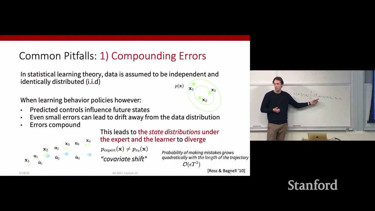
Closed-loop distribution shift causes naive behavior cloning errors to compound quadratically at O(epsilon * T^2) over horizon T under a discrete per-step error probability epsilon. (5:02)
DAgger resolves covariate shift by iteratively executing the learned policy on the robot, querying an expert for corrective actions on the newly visited states, and retraining on the aggregated dataset. (15:58)
To prevent catastrophic mode averaging under Mean Squared Error on multimodal behaviors, modern imitation learning uses expressive generative frameworks including autoregressive transformers, diffusion policies, and flow matching. (52:34)
Action chunking outputs multi-step trajectory sequences rather than single Markovian steps, providing computational headroom for asynchronous execution and eliminating high-frequency sampling jitter. (60:05)
Inverse Reinforcement Learning frames imitation as inferring an unknown reward function optimized by the expert, but remains fundamentally challenged by reward ambiguity where multiple reward formulations yield identical policies. (76:37)
Detailed notes
## Background
Published on YouTube by Stanford Online on August 13, 2026, this video presents Lecture 15 of the Stanford University course AA203: Optimal and Learning-Based Control for the Spring 2026 term. Delivered by Dr. Daniele Gammelli and co-instructed with Prof. Marco Pavone, the session covers imitation learning and accompanies the open-access textbook Principles of Robot Autonomy.
## TL;DR
Dr. Daniele Gammelli examines the transition from classical optimal control to learning-based control, focusing on behavior cloning and inverse reinforcement learning. He explains why standard supervised learning fails in closed-loop environments due to covariate shift, compounding trajectory errors scaling as O(epsilon * T^2), and mode averaging over multimodal demonstrations. The lecture surveys algorithmic remedies including DAgger, camera-based data augmentation, and history conditioning, before exploring advanced generative policy parameterizations such as Gaussian mixture models, autoregressive transformers, diffusion policies, flow matching, and action chunking. It concludes with trajectory performance filtering, goal conditioning, and the alternating optimization foundations of Inverse Reinforcement Learning.
## Atmosphere & style
The lecture maintains a rigorous, lucid, and pragmatic academic tone typical of high-level graduate engineering courses. Dr. Daniele Gammelli lectures with an engaging, analytical cadence, punctuating formal mathematical formulations with direct rhetorical questions, intuitive diagrams, and real-world robotics war stories from autonomous driving and aerial drone research. Watching the session feels methodically structured and insightful, guiding viewers from the catastrophic breakdown of naive supervised baselines to the engineering elegance of modern generative physical AI models.
## Bulletin
- [05:02](https://www.youtube.com/watch?v=udHX5Auj7ik&t=302s) Closed-loop distribution shift causes naive behavior cloning errors to compound quadratically at O(epsilon * T^2) over horizon T under a discrete per-step error probability epsilon.
- [15:58](https://www.youtube.com/watch?v=udHX5Auj7ik&t=958s) DAgger resolves covariate shift by iteratively executing the learned policy on the robot, querying an expert for corrective actions on the newly visited states, and retraining on the aggregated dataset.
- [52:34](https://www.youtube.com/watch?v=udHX5Auj7ik&t=3154s) To prevent catastrophic mode averaging under Mean Squared Error on multimodal behaviors, modern imitation learning uses expressive generative frameworks including autoregressive transformers, diffusion policies, and flow matching.
- [01:00:05](https://www.youtube.com/watch?v=udHX5Auj7ik&t=3605s) Action chunking outputs multi-step trajectory sequences rather than single Markovian steps, providing computational headroom for asynchronous execution and eliminating high-frequency sampling jitter.
- [01:16:37](https://www.youtube.com/watch?v=udHX5Auj7ik&t=4597s) Inverse Reinforcement Learning frames imitation as inferring an unknown reward function optimized by the expert, but remains fundamentally challenged by reward ambiguity where multiple reward formulations yield identical policies.
## Key takeaways
- [03:10](https://www.youtube.com/watch?v=udHX5Auj7ik&t=190s) Behavior cloning frames policy learning as empirical risk minimization over expert state-action pairs, but standard supervised learning breaks down in closed-loop systems because policy execution alters future state distributions.
- [05:02](https://www.youtube.com/watch?v=udHX5Auj7ik&t=302s) Covariate shift causes the policy's visited state distribution to drift away from expert demonstrations, leading cumulative trajectory deviation to scale quadratically as O(epsilon * T^2).
- [09:58](https://www.youtube.com/watch?v=udHX5Auj7ik&t=598s) In multimodal scenarios where multiple valid maneuvers exist, minimizing Mean Squared Error produces the conditional expectation of actions, dangerously averaging distinct strategies into an invalid midpoint.
- [14:04](https://www.youtube.com/watch?v=udHX5Auj7ik&t=844s) Training purely on narrow, flawless expert demonstrations degrades real-world performance because policies never observe recovery actions from off-nominal states.
- [15:58](https://www.youtube.com/watch?v=udHX5Auj7ik&t=958s) DAgger iteratively rolls out the current policy to sample its own distribution, relabels visited states with expert corrective actions, and retrains the policy to suppress drift.
- [20:05](https://www.youtube.com/watch?v=udHX5Auj7ik&t=1205s) DAgger can serve as policy distillation, converting computationally expensive trajectory optimization or indirect optimal control solvers into high-speed feedforward neural networks.
- [26:26](https://www.youtube.com/watch?v=udHX5Auj7ik&t=1586s) Synthetic data augmentation, such as NVIDIA's three-camera vehicle rig, generates recovery data without staging physical crashes by labeling off-center sensor streams with corrective steering trajectories.
- [30:35](https://www.youtube.com/watch?v=udHX5Auj7ik&t=1835s) Imitation learning is fundamentally bounded by the demonstrator's competence and data distribution, requiring reinforcement learning to discover behaviors beyond human demonstrations.
- [35:03](https://www.youtube.com/watch?v=udHX5Auj7ik&t=2103s) Partial observability in single raw sensor frames can be resolved by conditioning policies on temporal observation histories using sequence models like transformers or RNNs.
- [46:12](https://www.youtube.com/watch?v=udHX5Auj7ik&t=2772s) Autoregressive action discretization applies the probability chain rule to decompose high-dimensional continuous action spaces into sequential 1D predictions, avoiding joint-grid sample sparsity at the cost of linear inference latency.
- [52:34](https://www.youtube.com/watch?v=udHX5Auj7ik&t=3154s) Diffusion policies and flow matching represent continuous multimodal distributions by learning to invert noise processes or map continuous vector fields, avoiding mode collapse without relying on discrete bins.
- [01:00:05](https://www.youtube.com/watch?v=udHX5Auj7ik&t=3605s) Action chunking predicts a sequence of future actions simultaneously, enabling asynchronous open-loop execution on hardware and enforcing temporal smoothness across control commands.
- [01:07:51](https://www.youtube.com/watch?v=udHX5Auj7ik&t=4071s) Suboptimal demonstration datasets can be made usable for behavior cloning via hard trajectory filtering or performance-weighted maximum likelihood estimation proportional to episodic returns.
- [01:12:45](https://www.youtube.com/watch?v=udHX5Auj7ik&t=4365s) Goal-conditioned behavior cloning turns arbitrary uncurated trajectories into useful training samples by treating reached terminal states as the intentional target goals.
- [01:15:34](https://www.youtube.com/watch?v=udHX5Auj7ik&t=4534s) Inverse Reinforcement Learning alternates between estimating parameterized reward functions that explain expert behavior and optimizing policies under those rewards, but must address ill-posed reward ambiguity.
## Detailed walkthrough
### [00:05](https://www.youtube.com/watch?v=udHX5Auj7ik&t=5s) Course Context and Roadmap: Learning-Based Optimal Control
The lecture opens with a review of the course trajectory in AA203. Having concluded the classical optimal control segment of the curriculum, the class has shifted into learning-based methods for optimal control. Previously, the focus centered on classical data-driven mechanisms—specifically system identification and adaptive control—before transitioning to a high-level conceptual framework for imitation learning and reinforcement learning. Dr. Daniele Gammelli notes that the goal has been to build a coherent mental model categorizing algorithms across these paradigms. This lecture zooms in directly on the imitation learning pillar.
```mermaid
flowchart TD
accTitle: Overview of Learning-Based Optimal Control Paradigms
accDescr: Flowchart showing the division of learning-based control into classical methods, reinforcement learning, and imitation learning branches.
subgraph LBC["Learning-Based Control"]
direction TB
C["Classical Methods\n(System ID, Adaptive Control)"]
RL["Reinforcement Learning"]
IL["Imitation Learning"]
end
subgraph IL_Branches["Imitation Learning Approaches"]
direction LR
BC["Behavior Cloning (BC)\nDirect policy learning: π_θ(u|x)"]
IRL["Inverse RL (IRL)\nReward inference: r(x, u)"]
end
IL --> BC
IL --> IRL
```
[01:05](https://www.youtube.com/watch?v=udHX5Auj7ik&t=65s) Imitation Learning: Behavior Cloning vs. Inverse Reinforcement Learning
Imitation learning serves as an umbrella term covering two primary schools of thought:
1. **Behavior Cloning (BC):** The learner assumes access to a dataset of state-control tuples $(x, u)$ gathered by observing an expert executing demonstrations in the real world. The core objective is to directly learn or approximate the expert's policy from this dataset. Concretely, one seeks a parameterized policy $\pi_\theta(u \mid x)$, parameterized by weights $\theta$, that represents a conditional distribution over controls given states.
2. **Inverse Reinforcement Learning (IRL):** Rather than mimicking actions directly, the objective is to uncover the underlying reward function or latent objective that the expert is implicitly optimizing. Here, the target of learning is a scalar reward function $r(x, u)$ that maps pairs of states and controls to a scalar measure of task success.
The roadmap for the day begins with behavior cloning, investigates its primary pitfalls and classical mitigation strategies, touches on related cloning paradigms, and concludes with inverse reinforcement learning.
[03:10](https://www.youtube.com/watch?v=udHX5Auj7ik&t=190s) Behavior Cloning as Supervised Learning: The Core Setup
Behavior cloning can be framed conceptually as supervised learning applied directly to behavior. In classical supervised learning, one trains a parametric mapping from an input space $\mathcal{X}$ to an output space $\mathcal{Y}$—such as mapping an RGB image of a cat to its categorical label—via loss minimization over collected data pairs:
Behavior cloning adopts the exact same skeleton: an agent collects a dataset of expert demonstrations and trains a policy mapping states to actions to optimize a chosen performance metric. However, Gammelli emphasizes the critical question: *"Does this work? And are we done?"*
In practice, direct supervised learning frequently breaks down in closed-loop systems. A naive mapping ignores the dynamical nature of real environments, leading to systematic failure modes that frontier research in robotics and learning-based control must explicitly mitigate.
[05:02](https://www.youtube.com/watch?v=udHX5Auj7ik&t=302s) Failure Mode 1: Compounding Errors and Covariate Shift
The first major breakdown stems from compounding errors. Statistical learning theory relies heavily on the Independent and Identically Distributed (I.I.D.) assumption, where models are trained and evaluated on samples drawn independently from a fixed distribution $p(x)$. In control, however, an agent is situated inside a dynamic closed loop: the predictive controls output by the policy actively dictate the future states the agent encounters.
When the learned policy commits even minor errors, those deviations feed back into the system, shifting the agent slightly off course. Over the temporal unrolling of a trajectory, these errors compound, steering the agent into unfamiliar regions of the state space where it was never trained to recover.
```mermaid
flowchart LR
accTitle: Compounding Error Feedback Loop
accDescr: Diagram illustrating how policy execution errors shift the state distribution away from expert coverage.
A["State x_t"] --> B["Policy π_θ(u|x)"]
B -->|"Prediction Error ε"| C["Suboptimal Control u_t"]
C --> D["Dynamics Step: x_t+1 ~ p(·|x_t, u_t)"]
D -->|"Covariate Shift"| E["Out-of-Distribution State x_t+1"]
E --> A
```
Formally, this discrepancy is known as **covariate shift**: the state distribution induced under the expert policy, $p_{\text{expert}}(x)$, diverges from the distribution induced under the learned learner policy, $p_{\pi_\theta}(x)$.
The expert state distribution is defined by the initial state distribution combined with the rollout of the expert policy $\pi^*$ through the environment dynamics:
Theoretical analyses show that if an agent has a probability $\epsilon$ of making an erroneous action decision at each step within a discrete action setting, the probability of total trajectory deviation does not scale linearly; it scales quadratically with the length of the time horizon, exhibiting an error growth on the order of:
$$\mathcal{O}(\epsilon T^2)$$
Addressing a student question regarding trajectory independence, Gammelli clarifies that while individual demonstration trajectories in the offline dataset may be treated as independent realizations, the problem being solved is learning an instantaneous feedback policy $u_t = \pi_\theta(x_t)$ that maps current states to controls in closed-loop execution.
[09:58](https://www.youtube.com/watch?v=udHX5Auj7ik&t=598s) Failure Mode 2: Multimodal Behavior and the Pitfall of Mean Squared Error
A second critical pitfall is **multimodal behavior**. In real-world control tasks, multiple distinct, equally valid solutions often exist for a single scenario.
Gammelli illustrates this with an intuitive physical example: flying an autonomous drone toward a tree. A human expert steering via joystick might swerve cleanly to the left in half of the demonstration runs and to the right in the remaining runs. Both trajectories are equally optimal.
```mermaid
flowchart TD
accTitle: Multimodal Failure Mode under Mean Squared Error
accDescr: Flowchart demonstrating how MSE averages two valid expert modes into a catastrophic failure mode.
subgraph Data["Expert Demonstrations"]
L["Mode 1: Fly Left of Obstacle"]
R["Mode 2: Fly Right of Obstacle"]
end
subgraph Fit["Standard Regression Fitting"]
MSE["Mean Squared Error (MSE) Loss\nmin E[(u - u*)^2]"]
end
subgraph Outcome["Learned Behavior"]
Avg["Averaged Prediction:\nFly Directly into Tree"]
end
L --> MSE
R --> MSE
MSE --> Outcome
```
If these demonstrations are pooled into a dataset, the underlying conditional control distribution $\pi^*(u \mid x)$ is bimodal:
- Attempting to fit this distribution using a standard neural network trained with a Mean Squared Error (MSE) loss creates a catastrophic failure mode.
- Mathematically, minimizing MSE encourages the model to output the conditional expectation $\mathbb{E}[u \mid x]$.
- For a bimodal distribution with peaks representing "steer left" and "steer right", the expected value is the algebraic mean: "fly straight."
Rather than choosing one valid mode or the other, an MSE-trained policy commands the drone to fly straight through the center, crashing directly into the tree. Standard regression objectives are fundamentally ill-suited for multi-modal demonstration distributions without structural modifications.
[12:14](https://www.youtube.com/watch?v=udHX5Auj7ik&t=734s) Multimodal Failure Modes and the Roadmap Ahead
Dr. Gammelli highlights the severe downside of naive supervised fitting when expert demonstrations exhibit multiple modes. If an algorithm attempts to minimize mean squared error across two valid modes, it does "probably the worst thing that we could do because it fits exactly in the middle," balancing out the errors between the trajectories and yielding an action that is catastrophic or invalid. This scenario arises routinely in robotics and autonomous systems whenever datasets are gathered from multiple human or algorithmic experts, each reacting differently to the identical environmental condition.
```mermaid
flowchart TD
accTitle: Multi-Pronged Remediation Framework
accDescr: Three core strategies to tackle compounding errors and policy multimodality.
subgraph S1["Compounding Errors"]
A["Algorithmic Solutions (e.g., DAgger)"]
B["Targeted Data Collection"]
end
subgraph S2["Multimodal Distributions"]
C["Expressive Model Classes"]
end
```
To structure the rest of the lecture, Dr. Gammelli outlines a three-part conceptual roadmap designed to remedy these foundational issues:
- **Algorithmic approaches:** Designing interactive imitation algorithms (such as data aggregation) specifically targeting the compounding error and covariate shift problem.
- **Data collection strategies:** Augmenting datasets and structuring rollouts to expose recovery behaviors.
- **Expressive model classes:** Deploying richer policy parameterizations (e.g., diffusion models or energy-based policies) capable of capturing multimodal distributions rather than averaging across distinct modes.
---
[14:04](https://www.youtube.com/watch?v=udHX5Auj7ik&t=844s) The Counterintuitive Paradox of Perfect Data
In conventional behavioral cloning, practitioners often fall into the trap of assuming that higher data quality strictly implies pristine demonstrations. The intuition seems obvious: to compile the performance of an expert into a parametric function, one should gather demonstrations that solve the task flawlessly. However, this creates a dataset confined to a razor-thin tube of the state space, showing only ideal task execution.
Once deployed in the real world, the learned policy will inevitably make minor tracking or control mistakes due to model capacity limits, noise, or unmodeled dynamics. In those unvisited off-distribution states, a policy trained solely on flawless demonstrations has no concept of recovery. Dr. Gammelli emphasizes that there is tremendous value in exposing the learner to mistakes: "learning from a broader set of trajectories that makes some mistakes but also shows ways to correct from these mistakes is, in general, more valuable than learning from a narrow set of perfect demonstrations."
---
[15:58](https://www.youtube.com/watch?v=udHX5Auj7ik&t=958s) The DAgger Algorithm and Iterative Relabeling
To systematically automate the collection of corrective demonstrations, Dr. Gammelli introduces **DAgger** (Dataset Aggregation), a widely studied imitation learning algorithm explicitly designed to eliminate covariate shift.
```mermaid
flowchart LR
accTitle: DAgger Algorithmic Loop
accDescr: Iterative process of rolling out learner policies, querying the expert, and aggregating data.
subgraph SG1["Learner Execution"]
P["Policy: pi_theta^i"] -->|"roll out"| T["Rollouts: (x_t, u_t^learner)"]
end
subgraph SG2["Expert Supervision"]
T -->|"query expert at x_t"| R["Relabeled: (x_t, u_t^expert)"]
end
subgraph SG3["Aggregation & Retraining"]
R -->|"merge into D"| D["Updated Dataset D"]
D -->|"supervised learning"| PNEW["Updated Policy: pi_theta^(i+1)"]
end
PNEW -.->|"next iteration"| P
```
DAgger operates through an iterative supervised learning loop:
1. **Initialization:** Start with an initial offline dataset $\mathcal{D}_1$ of expert trajectories and train an initial policy $\pi_\theta^1$.
2. **Rollout:** Let the current learner policy $\pi_\theta^i$ interact directly with the environment, executing its own actions and visiting states drawn from its induced state distribution $p_{\pi_\theta^i}(x)$.
3. **Expert Relabeling:** Take the visited states $x_t$ along these rollouts and query the expert for the corrective action: replace the control executed by the learner, $u_t^{\text{learner}}$, with the control the expert would have chosen, $u_t^{\text{expert}} = \pi^*(x_t)$.
4. **Data Aggregation:** Assemble this new dataset $\mathcal{D}^i = \{(x_t, u_t^{\text{expert}})\}$ and aggregate it with the running dataset, $\mathcal{D} \leftarrow \mathcal{D} \cup \mathcal{D}^i$.
5. **Policy Update:** Retrain the policy on the expanded aggregated dataset $\mathcal{D}$ to produce $\pi_\theta^{i+1}$, then repeat.
Because the expert is evaluated strictly on the states $x_t \sim p_{\pi_\theta}(x)$ visited by the evolving learner, DAgger eliminates the train-test mismatch by directly bridging the state distribution gap.
---
[20:05](https://www.youtube.com/watch?v=udHX5Auj7ik&t=1205s) Human-in-the-Loop Interventions and Practical Trade-offs
A student raises a question regarding the mechanics of expert relabeling: if the expert is an actual human supervisor, does relabeling force the human to step through discrete states one by one offline to assign controls, or does it require continuous supervision?
Dr. Gammelli explains that the algorithm presented so far is "DAgger v0"—the baseline formulation. In physical robotic systems, an extension called **Human-Gated DAgger** (or intervention-based DAgger) is often favored:
- A robotic arm executes a task autonomously while a human overseer monitors it in real time.
- As long as the robot behaves properly, the learner remains in control.
- When the arm is about to make a critical error (such as knocking over an object or spilling a container), the human intervenes, takes over teleoperation, and guides the arm along a recovery path back to the task distribution.
- The intervened trajectory segment is collected and aggregated, allowing the system to explore new recovery trajectories rather than freezing the state path to identical pre-recorded points.
Dr. Gammelli concludes by assessing DAgger's efficiency trade-off. At a conceptual level, DAgger is highly data-efficient because it selectively queries the expert only in the exact failure-prone regions visited by the policy, rather than requiring brute-force coverage across every conceivable state. However, because online expert queries—especially from human operators—can be prohibitively slow and expensive, whether DAgger is practical depends heavily on whether a fast, low-cost expert (like an algorithmic planner or simulator) is available.
[24:30](https://www.youtube.com/watch?v=udHX5Auj7ik&t=1470s) Variations on DAgger and Policy Distillation
Dr. Gammelli transitions from the standard, textbook implementation of DAgger (Dataset Aggregation) to several practical variations designed to alleviate its heavy labeling burden. In the naive version of DAgger, the expert must be queried across all states visited by the learner during policy rollouts, which can quickly become intractable or prohibitively expensive. To address this, one common modification is a confidence-based approach: instead of blanketing the expert with queries, the system monitors a measure of the learner's own predictive uncertainty and selectively requests expert intervention only in states where the policy lacks confidence. Another widely used variant is "human-gated DAgger," where a human supervisor monitors the learner during execution and takes control or injects labels only when an overt mistake or hazardous condition occurs.
A student asks whether the underlying motivation for running these algorithms is to produce a lighter, faster policy for online execution when an expert policy is already available. Dr. Gammelli confirms that execution speed is indeed a major driver. Taking a broader perspective across the entire course, he explains that while modern robotics is increasingly shifting toward end-to-end and learning-based architectures, generating dependable supervision for these models—even in frontier AI systems—still relies heavily on classical control methods. Algorithms like DAgger can effectively be viewed as mechanisms for "distilling some maybe extremely expensive indirect method for optimal control into a fast neural network that can approximate it" in real time.
- **Confidence-based DAgger:** Uses an internal uncertainty metric from the learning policy to query the expert selectively rather than uniformly across every visited state.
- **Human-gated DAgger:** Involves human-in-the-loop oversight where human supervisors intervene dynamically only when the learner makes an error.
- **Distillation Motivation:** Replaces computationally burdensome trajectory optimization or indirect optimal control solvers with an efficient feedforward neural network capable of real-time onboard inference.
---
[26:26](https://www.youtube.com/watch?v=udHX5Auj7ik&t=1586s) Data Augmentation for Covariate Shift: NVIDIA's 2016 Autonomous Driving Study
Shifting from algorithmic solutions like DAgger to data-centric strategies, Dr. Gammelli presents empirical case studies illustrating how intentional data collection and augmentation can neutralize covariate shift. The first case study is NVIDIA’s pioneering 2016 autonomous driving project. In this early deep learning deployment, researchers trained a convolutional neural network (CNN) to directly predict vehicle steering wheel angles from forward-facing onboard camera imagery. Early iterations demonstrated poor and potentially dangerous handling, but scaling up human demonstrations—recording pairs of camera frames and driver steering commands—eventually yielded remarkably stable lane-following behavior.
Dr. Gammelli emphasizes that the critical innovation of the NVIDIA study was not merely the neural network architecture, but a clever data augmentation trick designed to combat compounding errors. Because human drivers rarely make severe mistakes during normal operations, training data naturally lacks examples of how to recover once the vehicle drifts off-center. Intentionally gathering real-world data of a car driving off the road and swerving back is both dangerous and expensive. NVIDIA solved this by outfitting the vehicle with three forward-facing cameras: one center, one left, and one right. While the center camera represented normal lane centering, the left and right camera feeds were treated as synthetic "mistakes." By treating an off-center side camera view as if it were the main front-facing view, engineers could artificially calculate and assign a corrective steering command to bring the car back toward the center of the lane.
```mermaid
flowchart TD
accTitle: Synthetic Data Augmentation via Multi-Camera Setup
accDescr: Flowchart illustrating how NVIDIA used three cameras to generate synthetic recovery trajectories to overcome covariate shift.
subgraph Capture["Multi-Camera Rig"]
L["Left Camera View"]
C["Center Camera View"]
R["Right Camera View"]
end
subgraph Augment["Synthetic Corrective Labeling"]
AL["Simulates Drift to Left Edge<br/>Label: Synthetic Steer Right"]
AC["Standard Nominal Trajectory<br/>Label: Ground-Truth Human Steer"]
AR["Simulates Drift to Right Edge<br/>Label: Synthetic Steer Left"]
end
subgraph Model["Policy Training"]
CNN["Convolutional Neural Network<br/>(Predicts Steering Angle)"]
end
L --> AL
C --> AC
R --> AR
AL --> CNN
AC --> CNN
AR --> CNN
```
- **Pioneering Study:** NVIDIA (circa 2016) demonstrated end-to-end behavioral cloning mapping raw pixel inputs to continuous steering angles.
- **The Core Problem:** Expert human drivers maintain the center of the lane, leaving the model with zero data on how to correct course after minor drift.
- **The Synthetic Recovery Trick:** Off-axis camera angles (left and right) simulate vehicle displacement, paired with synthetic steering offsets that direct the vehicle back into the lane center without risking hardware in real-world crashes.
---
[30:35](https://www.youtube.com/watch?v=udHX5Auj7ik&t=1835s) The GoPro Headband Hike and the Limits of Imitation Learning
Dr. Gammelli illustrates how this same principle reappeared in a robotics study from the University of Zurich, where researchers trained autonomous quadrotors to follow hiking trails through the Swiss Alps using vision. Rather than continuous steering commands, this system mapped incoming camera frames to a discrete action distribution: "go straight," "turn left," or "turn right." To collect data safely without crashing drones into trees, the researchers strapped a headband equipped with three GoPros onto their heads and simply walked the mountain trails.
Just as in the NVIDIA system, the multi-camera setup provided automatic corrective supervision. The center GoPro feed was labeled as a nominal "go straight" action, while views from the left and right cameras simulated deviations off the trail and were automatically labeled with corrective commands—the left camera was labeled as "turn right" and the right camera as "turn left." Dr. Gammelli highlights the unifying lesson across both case studies: addressing covariate shift requires being deliberate about data collection by intentionally embedding mistakes and recovery maneuvers into the dataset, either synthetically through sensor geometry or algorithmically via systems like DAgger.
A student asks whether imitation learning allows one to decouple drone decision-making from the physical dynamics of the human carrying the sensors—for instance, allowing a drone to climb two feet higher over a tree branch instead of being restricted to walking paths. Dr. Gammelli explains that pure imitation learning cannot achieve this:
> "In imitation learning, we are, again, at face value, trying to approximate and imitate the behavior of some expert. And that's about it. So we don't really want to go beyond what the expert is able to do. And we typically won't have access to data that is beyond what the expert is able to experience."
He notes that discovering novel maneuvers or exploiting dynamics beyond human capabilities is the explicit domain of reinforcement learning, where an agent can interact directly with an environment or physics simulator and discover better strategies through trial and error.
- **University of Zurich Trail Navigation:** Quadrotors learned trail navigation from a three-GoPro headband worn by hikers in the Swiss mountains.
- **Discrete Classification:** The network outputs probabilities across three distinct actions: straight, turn left, and turn right.
- **Intentional Mistake Injection:** Both the car and drone setups artificially generate "out-of-distribution" recovery samples without placing platforms in physical danger.
- **Scope of Imitation Learning:** IL is bounded strictly by the behavior and distribution of the demonstrations; exceeding demonstrator dynamics requires reinforcement learning.
---
[35:03](https://www.youtube.com/watch?v=udHX5Auj7ik&t=2103s) Addressing Multimodal Behavior and Partial Observability with History
Having addressed covariate shift through algorithms and data collection, Dr. Gammelli introduces the next major hurdle in imitation learning: handling multimodal behavior. When demonstrators can execute multiple valid, distinct actions in the exact same state, standard regression objectives tend to average those modes together, leading to catastrophic decisions (such as steering straight into an obstacle when deciding whether to pass on the left or right). Dr. Gammelli outlines two primary families of methods to tackle this: conditioning policies on a history of past observations, and deploying expressive function classes (such as mixture models or diffusion policies) that can represent multimodal probability distributions.
Focusing first on observation histories, Dr. Gammelli points out a critical gap between theory and practice. Throughout earlier optimal control lectures, the system state was treated as fully Markovian—a complete representation that encapsulates all past historical information. However, when working with real robotic systems operating on raw sensor inputs like camera images, policies deal with partial observations rather than ground-truth system states.
Under behavioral cloning, defining a policy strictly over the instantaneous observation $x_t$ assumes that a human demonstrator will always take the exact same action when presented with an identical image. In practice, demonstrators possess internal intent and dynamic context that are completely invisible in a single snapshot. By appending a sequence of past observations into the policy's conditioning context, the model can disambiguate hidden states and resolve what would otherwise appear to be conflicting, multimodal behaviors.
- **Multimodality Challenge:** Unimodal loss functions average distinct valid modes, leading to disastrous failure modes in ambiguous environments.
- **Markov Assumption vs. Reality:** Ground-truth states contain all past information, but real-world vision systems deal with partial observations in a partially observable Markov decision process (POMDP) setting.
- **History as Context:** Conditioning policies on observation sequences $\tau_{t-k:t}$ provides context that disambiguates demonstrator intent and breaks confounding symmetries in single-frame observations.
[37:26](https://www.youtube.com/watch?v=udHX5Auj7ik&t=2246s) Overcoming Non-Markovian Observations with History and Sequence Models
Dr. Daniele Gammelli opens by addressing a fundamental limitation in naive behavioral cloning setups where observations lack crucial temporal context. If a vehicle's state $x$ is defined solely as the current frame from a front-facing camera and the control action $u$ is the steering angle, a single snapshot cannot reveal vehicle speed, acceleration, or other dynamic quantities essential for decision-making. Relying on an isolated snapshot implicitly assumes that identical camera frames must always trigger identical control actions, ignoring latent temporal dynamics. By contrast, conditioning the policy on a history of sequential observations allows the system to extract velocity, intent, and scene evolution over time.
In modern robot autonomy, incorporating historical observations is standard practice and relies on sequence models. Depending on the architecture, practitioners deploy transformers, recurrent neural networks (RNNs), or temporal convolutional networks to process sequences of past states or observations and output the next control action. Dr. Gammelli emphasizes that choosing the length of this temporal history is rarely guided by strict theory; rather, it is "usually very empirical." In real-world projects, engineers conduct ablation studies—training candidate policies on the same dataset while varying the number of historical look-back steps—to determine what empirically yields the best performance.
```mermaid
flowchart LR
accTitle: Sequence Policy Architecture
accDescr: Sequence of image observations fed into a sequence model to predict steering action.
subgraph InputHistory ["Observation History"]
O1["Image x(t-2)"]
O2["Image x(t-1)"]
O3["Image x(t)"]
end
subgraph Model ["Sequence Model"]
SM["Transformer / RNN"]
end
subgraph Action ["Control Output"]
U["Action u(t) (Steering)"]
end
O1 --> SM
O2 --> SM
O3 --> SM
SM --> U
```
[39:03](https://www.youtube.com/watch?v=udHX5Auj7ik&t=2343s) Representing Full Distributions: Discrete vs. Continuous Formulations
Dr. Gammelli shifts focus to a core challenge in imitation learning: capturing the full data distribution rather than collapsing to an uninformative mean. Recalling the motivating scenario of a drone flying past a tree—where dodging left or dodging right represent two equally valid, distinct behavioral modes—averaging the modes leads directly to a catastrophic collision with the tree trunk. The policy must therefore model the entire multimodal distribution $p(u \mid x)$. Doing so requires careful consideration of whether the target action distribution is formulated as discrete or continuous.
```mermaid
flowchart TD
accTitle: Policy Distribution Representations
accDescr: Branching pathways comparing discrete classification to continuous parametric outputs.
Root["Policy Distribution p(u|x)"] --> Disc["Discrete Formulations"]
Root --> Cont["Continuous Formulations"]
Disc --> DiscPros["Natural multi-modality<br/>Standard cross-entropy loss"]
Disc --> DiscCons["Poor scaling in high dimensions<br/>Curse of dimensionality"]
To output a parametric distribution, a neural network is structured to predict distribution parameters:
- **Discrete outputs**: The network predicts unnormalized logits or categorical probabilities over a finite action set (e.g., cardinal movements: up, down, left, right), or across discretized bins over a continuous action space. This formulation naturally captures multi-modality and trains cleanly via standard categorical cross-entropy loss. However, its primary downside is poor scalability: as action dimensionality increases, the required number of bins explodes exponentially.
- **Continuous outputs**: The network predicts the parameters of an analytical continuous density (e.g., the mean $\mu$ and covariance/standard deviation $\sigma$ of a Gaussian over steering angles). While continuous distributions bypass discretization artifacts and represent continuous control smoothly, single unimodal Gaussians lack expressive power; attempting to fit a unimodal Gaussian to bimodal data forces it to position its mean directly between the modes, failing to replicate true expert behavior.
[43:36](https://www.youtube.com/watch?v=udHX5Auj7ik&t=2616s) Multimodal Continuous Actions via Gaussian Mixture Models (GMMs)
When an audience member asks whether continuous scaling also suffers in higher dimensions and whether adding mixture components can capture multiple modes, Dr. Gammelli notes that while high-dimensional continuous distributions can scale better than brute-force multidimensional grid binning (since an $n$-dimensional Gaussian is compactly parameterized by a mean vector and a covariance matrix), expressiveness remains the bottleneck. This leads directly to Gaussian Mixture Models (GMMs).
Instead of fitting a single Gaussian, a GMM expresses the policy as a convex combination of $k$ distinct Gaussian components:
Each component has its own mean $\mu_i$ and covariance matrix $\Sigma_i$, weighted by categorical mixture coefficients $w_i$. This enables flexible approximation of complex, multimodal distributions by combining relatively simple primitives. However, selecting the number of components $k$ introduces hyperparameter challenges:
- Choosing $k$ too high risks overfitting the training demonstrations, yielding poor generalization at test time.
- Choosing $k$ too low underfits and fails to separate distinct behavioral modes.
- While domain knowledge can occasionally dictate $k$ (e.g., knowing an autonomous vehicle possesses exactly three discrete maneuvers around an obstacle), $k$ remains largely an empirical tuning parameter.
[46:12](https://www.youtube.com/watch?v=udHX5Auj7ik&t=2772s) Autoregressive Discretization and Transformer Policies
To retain the multimodal flexibility of discrete representations without suffering the combinatorial explosion of high-dimensional grids, Dr. Gammelli introduces the discretized autoregressive approach. In a joint two-dimensional action space $(x_1, x_2)$, naively discretizing the entire 2D plane creates an exhaustive grid where estimating probability densities requires learning a distinct parameter for every cell. Beyond the massive parameter count, this suffers severely from the curse of dimensionality during sample-based learning: populating all 2D bins accurately requires an exponentially large demonstration dataset, leaving most cells unvisited.
```mermaid
flowchart LR
accTitle: Joint vs Autoregressive Decomposition
accDescr: Comparison of a dense 2D joint grid versus an autoregressive factorization into 1D conditional distributions.
subgraph DirectJoint ["Direct 2D Discretization (Exponential)"]
J["p(x1, x2) on 2D Grid<br/>N x N bins, sparse data"]
end
subgraph AutoregressiveDecomp ["Autoregressive Factorization (Linear)"]
F1["Factor 1: p(x1)<br/>N bins (dense)"]
F2["Factor 2: p(x2 | x1)<br/>N bins (dense)"]
F1 --> F2
end
```
By applying the probability chain rule, the joint distribution is factored exactly into a product of conditional 1D distributions:
$$p(x_1, x_2) = p(x_1) \, p(x_2 \mid x_1)$$
This exact decomposition replaces an $N \times N$ two-dimensional grid with sequential 1D discrete models:
- Discretizing along one dimension at a time dramatically reduces total parameter counts.
- Sample efficiency improves substantially because the exact same training demonstrations appear significantly denser when projected onto 1D marginals rather than scattered sparsely across a high-dimensional joint grid.
This autoregressive formulation directly reflects how modern generative transformer architectures operate in robot control policies. In large language models (LLMs), a transformer takes context tokens, outputs a categorical distribution over the next token $x_t$, samples or predicts it, and feeds it autoregressively back into the model to predict $x_{t+1}$. Robotics policies adopt the exact same framework: conditioned on task context (such as camera images or natural language task instructions), the policy decomposes continuous action vectors into discretized tokens and autoregressively predicts each dimension one step at a time.
[51:13](https://www.youtube.com/watch?v=udHX5Auj7ik&t=3073s) Autoregressive Action Prediction and the Compute Trade-off
Dr. Daniele Gammelli illustrates how autoregressive modeling—the foundational mechanism behind Large Language Models (LLMs)—can be applied directly to multi-dimensional action spaces in robot control. Rather than outputting all control commands simultaneously, the policy breaks down an action vector dimension by dimension. For instance, in an autonomous driving setup where the control vector $u$ comprises steering angle and acceleration, the model can first predict the steering angle, feed that predicted steering value back into the network as input, and subsequently predict the acceleration.
A student asks whether this approach implies that one must explicitly unpack and understand all inter-dimensional dependencies before running inference to narrow down the action space. Gammelli clarifies that high dimensionality itself is not the barrier; instead, the fundamental trade-off is "ease of representation with compute." Under an autoregressive formulation, you cannot sample the entire action vector in a single forward pass. Generating an $n$-dimensional action vector requires $n$ sequential calls to the network (such as a transformer block), scaling the computational budget directly with the number of control dimensions.
- **Autoregressive action decomposition**: Predicts $u^{(1)}$, feeds $u^{(1)}$ back into the model to predict $u^{(2)}$, iterating until all $n$ dimensions of action vector $u$ are generated.
- **Computational cost**: Requires $n$ distinct sequential evaluation steps (or transformer passes) per control step, increasing latency relative to single-shot prediction.
---
[52:34](https://www.youtube.com/watch?v=udHX5Auj7ik&t=3154s) Diffusion Models: Transforming Noise to Multi-Modal Actions
Gammelli shifts focus to another dominant class of generative architectures: diffusion models and flow matching. In imitation learning, policies often need to capture complex, multi-modal behavior distributions that cannot be sampled directly. Diffusion circumvents this challenge by defining a transport mechanism from a tractable reference distribution—such as a standard Gaussian from which sampling is trivial—to the wild, arbitrary target distribution.
Originally developed for high-fidelity image generation (such as mapping conditioning text like "generate an image of a cat" to pixels), diffusion defines two opposite processes:
1. **Forward process (training data preparation)**: Starting with an uncorrupted data point $x_0$, Gaussian noise is gradually and iteratively injected across time steps ($x_0 \to x_1 \to x_2 \dots$) until the data is completely degraded into pure isotropic noise.
2. **Reverse process (sampling/inference)**: Beginning from a pure noise sample, a learned parametric model $f_\theta$ predicts and removes the injected noise term $\epsilon$ step-by-step, gradually recovering the target sample.
While acknowledging that this conceptual overview is somewhat high-level, Gammelli emphasizes that diffusion processes provide an exceptionally expressive tool for representing multi-modal action distributions without falling into mode averaging.
---
[56:13](https://www.youtube.com/watch?v=udHX5Auj7ik&t=3373s) Flow Matching: Vector Fields and Straight-Line Transport
Moving to more recent advances, Gammelli explains flow matching as an elegant alternative to classical diffusion. Instead of learning an error term $\epsilon$ to perform step-by-step stochastic denoising, flow matching models statistical transport by learning a deterministic continuous vector field $v_\theta$. The vector field guides probability mass from the simple noise distribution straight into the complex target distribution.
```mermaid
flowchart LR
accTitle: Flow Matching Training and Inference
accDescr: Diagram illustrating flow matching training via velocity regression and inference via forward integration.
subgraph Train["Training Phase"]
A["Prior Sample x₀ ~ N(0, I)"] --> C["Linear Interpolation xₜ"]
B["Target Data x₁ ~ p_data"] --> C
C --> D["Target Velocity (x₁ - x₀)"]
D --> E["Regress Vector Field v_θ(xₜ, t)"]
end
subgraph Infer["Inference Phase"]
F["Noise Sample x₀"] --> G["Integrate v_θ via Euler Steps"]
G --> H["Target Action Sample x₁"]
end
```
The mathematical formulation and runtime execution operate as follows:
* **Training phase**: Sample an initial noise point $x_0 \sim \mathcal{N}(0, I)$, a target data point $x_1$ from the demonstration dataset, and a normalized time step $t \sim \mathcal{U}(0, 1)$. The method draws a straight line between $x_0$ and $x_1$ via linear interpolation. The ground-truth velocity between these points is simply $x_1 - x_0$. The model parameters $\theta$ are trained by minimizing the regression loss between the predicted velocity $v_\theta(x_t, t)$ and the target velocity $(x_1 - x_0)$.
* **Inference phase**: Sample an initial point $x_0$ from the Gaussian prior and integrate forward along the learned vector field $v_\theta$ (using standard numerical integrators like Euler integration) from $t=0$ to $t=1$ to synthesize a sample from the target distribution.
Flow matching has gained widespread traction because of its simulation efficiency and its natural ability to model continuous probability distributions, making it particularly well suited for robotic control tasks.
---
[01:00:05](https://www.youtube.com/watch?v=udHX5Auj7ik&t=3605s) Action Chunking and Smoother Policy Execution
Gammelli introduces "action chunking," describing it as essential "trick of the trade" and currently the most popular way to parameterize robot learning policies. Traditionally, feedback policies have been framed in a purely Markovian loop: at time step $t$, observe state $x_t$, sample a single control action $u_t \sim \pi(u_t \mid x_t)$, execute that action in the environment, transition to state $x_{t+1}$, and repeat. Action chunking shifts this paradigm by predicting an entire sequence of future actions over a planning horizon of length $k$ ($u_t, u_{t+1}, \dots, u_{t+k-1}$) simultaneously, bearing a strong conceptual resemblance to Model Predictive Control (MPC).
This architectural design offers two major practical advantages:
1. **Computational headroom for inference**: Deep generative models (like diffusion policies or large transformers) have non-trivial inference latency. Pre-computing a chunk of $k$ future actions allows the robot to execute those open-loop steps while providing ample time to compute the next chunk asynchronously.
2. **Trajectory smoothness and temporal coherence**: Calling an imperfect learned stochastic policy $\pi_\theta$ at every single time step introduces random sampling noise and high-frequency jitter. Predicting a multi-step trajectory chunk enforces strong temporal correlation among successive controls, yielding smoother motions that transfer far better to physical hardware.
---
[01:03:04](https://www.youtube.com/watch?v=udHX5Auj7ik&t=3784s) Real-World Architectures: Diffusion Policy and Robotics Transformers
To connect these generative concepts to empirical robotic systems, Gammelli highlights landmark policy architectures:
* **Diffusion Policy**: Introduced as a foundational framework scaling diffusion processes to robotic manipulation, Diffusion Policy maps visual observations directly to full action trajectory chunks using a diffusion backbone. Gammelli highlights that by uniting expressive multi-modal generative modeling with action chunking, the model succeeded across highly complex manipulation tasks and exhibited strong generalization across varying environment conditions.
* **Robotics Transformer (RT series)**: A family of vision-language-action foundation models that use transformer architectures to map multimodal sensor inputs directly into control commands, illustrating how large-scale autoregressive and sequence-prediction techniques are deployed in modern physical AI.
[01:04:22](https://www.youtube.com/watch?v=udHX5Auj7ik&t=3862s) Summary of Behavior Cloning: Strengths, Pitfalls, and Trade-offs
Recapping recent architectural paradigms in imitation learning, policies often map from a historical buffer of sensor inputs (such as past image observations) alongside a high-level natural language instruction to output discretized actions. In robotic manipulation systems—such as multi-axis robotic arms executing continuous joint movements—this frequently involves discretizing continuous action dimensions and decoding them sequentially via autoregressive generation, conditioning each action component on previously decoded values.
```mermaid
flowchart LR
accTitle: Autoregressive Action Generation from Multi-Modal History
accDescr: Pipeline mapping image history and language prompts to sequential discretized action dimensions.
subgraph Inputs["Conditioning Inputs"]
H["Image History\n(Past Frames)"]
L["Language Task\nDescription"]
end
subgraph Model["Autoregressive Policy"]
D1["Action Dim 1\n(Discretized)"]
D2["Action Dim 2\n(Discretized)"]
Dn["Action Dim N\n(Discretized)"]
end
Inputs --> D1
D1 --> D2
D2 --> Dn
```
Stepping back to review the broader landscape, the central challenge in imitation learning revolves around mitigating critical pitfalls. Algorithmic interventions such as DAgger directly tackle distributional drift by collecting online policy rollouts queried against an expert, while smart data collection schemes (e.g., three-camera stereo setups accompanied by synthetic perturbed augmentations) inject recovery signals into the training distribution. A foundational emphasis lies in properly capturing multi-modal data distributions—whether via mixture density models, energy-based representations, or diffusion—to mirror true expert behaviors rather than collapsing onto arbitrary averages.
At its core, standard behavior cloning functions as supervised learning, bringing substantial engineering and computational benefits:
- **Optimization stability:** Supervised objectives are straightforward to implement, well-behaved under standard stochastic gradient descent, and monitorable via clean empirical loss metrics.
- **Sample efficiency:** It eliminates costly online trial-and-error environmental interactions, bypassing the sample complexity inherent to reinforcement learning.
- **No reward engineering:** It avoids the need to hand-specify numeric scalar reward signals. In complex real-world tasks like autonomous driving, defining an objective numeric metric for "good driving" is exceptionally hard, whereas gathering human driving demonstrations to mimic is comparatively tractable.
Conversely, behavior cloning suffers from deep structural drawbacks:
- **Strict dependence on demonstration quality:** The learned policy strictly mirrors the supervisor; if the training trajectories contain poor driving or erratic actions, the learned model will perform poorly.
- **Compounding distribution shift:** Although smart augmentations alleviate error accumulation, deviations from the training distribution remain an open generalization challenge.
- **Absence of exploration:** Because behavior cloning purely mimics historical data, it possesses no mechanism to explore or discover novel trajectories superior to those provided by the demonstrator.
---
[01:07:51](https://www.youtube.com/watch?v=udHX5Auj7ik&t=4071s) Beyond Pure Imitation: Suboptimal Data, Filtering, and Weighting
To bridge the gap between pure imitation and the performance optimization characteristic of reinforcement learning, modern methods adapt behavior cloning principles to approximate RL objectives without full trial-and-error loops. Rather than restricting datasets exclusively to strictly optimal expert demonstrations, these frameworks leverage broader, diverse datasets containing suboptimal runs, historical logs, or related secondary tasks, extracting high-performing policies through data selection or policy reconditioning.
```mermaid
flowchart TD
accTitle: Performance-Aware Behavioral Cloning Taxonomy
accDescr: Classification of methods that reintroduce scalar rewards into behavior cloning pipelines.
Dataset["Mixed / Suboptimal Demonstrations"]
Dataset --> Filter["Hard Filtering\nDiscard rollouts where\nTotal Reward < r̄"]
Dataset --> Reweight["Sample Reweighting\nScale MLE loss by\nPerformance / Reward w(τ)"]
Dataset --> Cond["Conditioned Policies\nCondition π(u|x, c) on\nTarget Goal or Target Return"]
```
When an underlying reward metric $r(x_t, u_t)$ is available to evaluate how well an action performed at state $x_t$, two primary strategies emerge:
1. **Hard Filtering:** Demonstrations are evaluated by their cumulative episodic return. A predefined threshold $\bar{r}$ filters out low-scoring runs, restricting standard behavior cloning exclusively to the subset of trajectories satisfying $\sum_t r(x_t, u_t) \ge \bar{r}$.
2. **Performance Weighting:** Rather than throwing out data, the maximum likelihood estimation (MLE) objective weights each trajectory's likelihood proportionally to its achieved return, shifting probability mass toward higher-performing behaviors rather than imitating every sample uniformly.
In response to a student question contrasting trajectory filtering against intentional data augmentation (which intentionally inserts off-distribution, suboptimal recovery states), the optimal approach depends heavily on the problem setting. Filtering is particularly advantageous when dealing with narrow, highly constrained manipulation tasks that do not demand manual recovery collection, or when handling massive, uncurated offline datasets where manual inspection is infeasible and toxic or failed rollouts must be purged algorithmically.
---
[01:12:45](https://www.youtube.com/watch?v=udHX5Auj7ik&t=4365s) Goal-Conditioned and Reward-Conditioned Policies
Rather than modeling a standard stationary policy distribution over controls conditioned purely on state, $\pi(u_t \mid x_t)$, an alternative paradigm enriches the conditioning variable:
$$\pi(u_t \mid x_t, c)$$
where $c$ represents an explicit target goal state $x_{\text{goal}}$ or an intended target return/performance metric $\hat{R}$.
Goal conditioning reframes the value of flawed demonstrations:
- A trajectory starting at $x_1$ and terminating at $x_T$ may fail the primary objective if $x_T \ne x_{\text{goal}}$.
- However, that identical rollout serves as a valid, successful demonstration of reaching any intermediate waypoint $x_i$ (or final state $x_T$) from earlier states along its path.
- By training a generalized goal-reaching policy parameterized by any arbitrary candidate target state $x_g$, *every* trajectory in an arbitrary offline dataset becomes a valid training example.
- At inference time, the system achieves the desired task simply by querying the universal goal-conditioned policy with the specific desired target state $x^*$.
- Similarly, reward-conditioned architectures train on trajectories tagged by their achieved returns, enabling practitioners at inference time to condition the policy on generating high-reward outcomes.
While behavior cloning aims to directly learn an action-generation policy that matches expert behavior, Inverse Reinforcement Learning (IRL) tackles the inverse system identification problem: uncovering the underlying objective function that the demonstrator was seeking to optimize.
- **Conceptual distinction:** Behavior cloning solves for $\pi_\theta(u \mid x) \approx \pi^*(u \mid x)$. IRL presumes the expert acts approximately optimal with respect to an unknown reward function $R_w(x, u)$ parameterized by weights $w$, and seeks to infer $w$.
- **General algorithmic template:** Most IRL formulations follow an iterative structure: proposing candidate reward parameters $w$, computing the induced optimal policy or trajectory distribution under that candidate reward, comparing the resulting behavior to empirical expert demonstrations, and updating $w$ to better explain why the expert chose their specific trajectory distribution.
[01:16:37](https://www.youtube.com/watch?v=udHX5Auj7ik&t=4597s) The Inverse Reinforcement Learning Loop and Reward Ambiguity
At a high level, the majority of Inverse Reinforcement Learning (IRL) algorithms operate by alternating between two iterative phases. The framework begins with an initial set of expert demonstrations alongside initialized parameters for both the reward function, parameterized by $w$, and the agent's policy, parameterized by $\theta$. The algorithm proceeds in a back-and-forth dance: in the first step, the parameters $w$ of the reward function are updated according to an objective that assesses how well that reward explains the demonstrated behavior. In the second step, the newly updated estimate of $w$ is used to optimize the policy parameters $\theta$ through standard reinforcement learning or planning, maximizing expected return under that inferred reward function. That revised policy is then fed back into the reward estimation step to further refine $w$, continuing the cycle until convergence.
```mermaid
flowchart LR
accTitle: Alternating Optimization in Inverse Reinforcement Learning
accDescr: Diagram illustrating the two alternating optimization steps between reward parameter updates and policy optimization in IRL.
subgraph IRL ["Iterative IRL Loop"]
direction TB
R["Update Reward Parameters (w)<br/>Fit objective to expert demonstrations"]
P["Optimize Policy Parameters (θ)<br/>Maximize expected return under current w"]
R -->|"Use updated w"| P
P -->|"Use updated policy"| R
end
```
Prominent algorithms in this space include Apprenticeship Learning, Maximum Margin Planning, and Maximum Entropy IRL. These algorithms fundamentally seek to resolve one of the most stubborn hurdles in inverse optimal control: reward ambiguity. Reward ambiguity refers to the ill-posed nature of IRL, where an infinite number of distinct reward functions—including the trivial reward that assigns zero to every state and action—can equally explain the observed expert trajectories. Each of these algorithmic frameworks incorporates specific structural priors and constraints into the two alternating optimization steps to break ties and ensure that the inferred reward genuinely captures the expert's underlying intent without collapsing into degenerate or ambiguous solutions.
- **Alternating Optimization:** Alternates between adjusting reward weights $w$ given the current policy and updating policy parameters $\theta$ given the current reward estimate.
- **Key Algorithms Mentioned:** Apprenticeship Learning, Maximum Margin Planning, and Maximum Entropy IRL.
- **Core Challenge:** Reward ambiguity, where numerous mathematical reward functions yield identical optimal trajectories on the same demonstration dataset.
---
[01:18:14](https://www.youtube.com/watch?v=udHX5Auj7ik&t=4694s) Lecture Summary: The Landscape of Imitation Learning
Dr. Gammelli wraps up the lecture by reviewing the broader mental model constructed over the course of the session for tackling imitation learning problems. The bulk of the discussion centered on behavior cloning, starting from the naive "v0" formulation that treats imitation purely as supervised regression: gathering a dataset of expert state-action pairs and training a function approximator to mimic those decisions directly. While conceptually straightforward, this naive version breaks down due to two principal failure modes: compounding distribution shift errors when the policy drifts away from the training distribution, and the inherent multi-modality of human or expert demonstrator behavior, where simple mean-seeking models collapse into dangerous compromises.
To overcome these roadblocks, several foundational paradigms were presented throughout the lecture:
- **Data Augmentation:** Crafting synthetic perturbations or multi-camera offsets during data collection so the model learns how to steer back toward nominal states.
- **Interactive Algorithms:** Deploying interactive collection schemes like DAgger (Dataset Aggregation) to solicit expert corrections on the learner's own induced state distribution.
- **Expressive Architectures:** Implementing expressive policy models capable of representing complex, multi-modal probability distributions rather than unimodal averages.
- **Alternative Formulations:** Framing policy extraction through reinforcement learning via supervised learning, as well as casting the task inversely via Inverse Reinforcement Learning to infer the underlying reward structure.
With these foundations established, Dr. Gammelli opens the floor for any final questions before concluding the session with a casual, "All right, then see you on Wednesday."
## Notable quotes
> [03:10](https://www.youtube.com/watch?v=udHX5Auj7ik&t=190s) Does this work? And are we done? — Dr. Daniele Gammelli
> [12:14](https://www.youtube.com/watch?v=udHX5Auj7ik&t=734s) probably the worst thing that we could do because it fits exactly in the middle — Dr. Daniele Gammelli
> [14:04](https://www.youtube.com/watch?v=udHX5Auj7ik&t=844s) learning from a broader set of trajectories that makes some mistakes but also shows ways to correct from these mistakes is, in general, more valuable than learning from a narrow set of perfect demonstrations. — Dr. Daniele Gammelli
> [24:30](https://www.youtube.com/watch?v=udHX5Auj7ik&t=1470s) distilling some maybe extremely expensive indirect method for optimal control into a fast neural network that can approximate it — Dr. Daniele Gammelli
> [30:35](https://www.youtube.com/watch?v=udHX5Auj7ik&t=1835s) In imitation learning, we are, again, at face value, trying to approximate and imitate the behavior of some expert. And that's about it. So we don't really want to go beyond what the expert is able to do. And we typically won't have access to data that is beyond what the expert is able to experience. — Dr. Daniele Gammelli
> [37:26](https://www.youtube.com/watch?v=udHX5Auj7ik&t=2246s) usually very empirical. — Dr. Daniele Gammelli
> [51:13](https://www.youtube.com/watch?v=udHX5Auj7ik&t=3073s) ease of representation with compute — Dr. Daniele Gammelli
> [52:34](https://www.youtube.com/watch?v=udHX5Auj7ik&t=3154s) generate an image of a cat — Dr. Daniele Gammelli
> [01:00:05](https://www.youtube.com/watch?v=udHX5Auj7ik&t=3605s) trick of the trade — Dr. Daniele Gammelli
> [01:04:22](https://www.youtube.com/watch?v=udHX5Auj7ik&t=3862s) good driving — Dr. Daniele Gammelli
> [01:18:14](https://www.youtube.com/watch?v=udHX5Auj7ik&t=4694s) v0 — Dr. Daniele Gammelli
> [01:18:14](https://www.youtube.com/watch?v=udHX5Auj7ik&t=4694s) All right, then see you on Wednesday. — Dr. Daniele Gammelli
## Mentioned
Dr. Daniele Gammelli, Prof. Marco Pavone, DAgger (Dataset Aggregation), NVIDIA, University of Zurich, GoPro, Gaussian Mixture Models (GMMs), Diffusion Policy, Robotics Transformer (RT series), Flow Matching, Model Predictive Control (MPC), Apprenticeship Learning, Maximum Margin Planning, Maximum Entropy IRL, Inverse Reinforcement Learning (IRL), Stanford University
## Video description
Lecture 15 — Imitation Learning
Read the companion textbook, Principles of Robot Autonomy, free online: https://porabook.com
To learn more about enrolling in AA203 Optimal and Learning-Based Control, visit: https://online.stanford.edu/courses/aa203-optimal-and-learning-based-control
Follow along with the course schedule and syllabus: https://stanfordasl.github.io/aa203/sp2526/
Bio: Dr. Daniele Gammelli is the Research Director of the Machine Intelligence for Robot Autonomy Laboratory at the Italian Institute of Artificial Intelligence (AI4I), and a Researcher in the Department of Aeronautics and Astronautics at Stanford University. Since 2022, he has been a Research Fellow at the Center for Aerospace Autonomy Research (CAESAR) at Stanford and, until 2025, at the Center for Automotive Research at Stanford (CARS). He received his Ph.D. in Machine Learning and Mathematical Optimization from the Technical University of Denmark (DTU) in 2022, where his doctoral thesis was nominated for the DTU Best Thesis of the Year Award and the DTU Young Researcher Award. Dr. Gammelli’s research focuses on developing the algorithmic foundations and system-level methodologies that enable AI-powered autonomous systems to operate safely, efficiently, and reliably in high-stakes environments, with an emphasis on aerospace autonomy and next-generation mobility systems.
Instructors:
Prof. Marco Pavone, Associate Professor of Aeronautics and Astronautics, Director of Autonomous Vehicle Research at NVIDIA
Dr. Daniele Gammelli, Research Director at the Italian Institute of Artificial Intelligence (AI4I), Researcher at the Department of Aeronautics and Astronautics, Stanford University
Full playlist: https://www.youtube.com/playlist?list=PLa9dmHsLK9dg
Dr. Daniele Gammelli frames imitation learning as a foundational paradigm of learning-based control, contrasting direct behavioral policy learning with reward inference while highlighting how compounding errors and multimodal demonstrations disrupt naive supervised imitation in closed-loop systems.
The Dual Pitfalls of Behavior Cloning (5:02)
Behavior cloning frames policy synthesis as supervised learning by training a parameterized policy $\pi_\theta(u \mid x)$ directly on expert state-action pairs $(x, u)$. In physical closed-loop systems, however, naive supervised fitting breaks down due to compounding errors and multimodal behaviors. Statistical learning assumes independent and identically distributed samples, but an agent's control actions directly dictate future states. Minor policy deviations alter the system's trajectory, causing the learner's state distribution $p_{\pi_\theta}(x)$ to diverge from the expert distribution $p_{\text{expert}}(x)$. This covariate shift leads to trajectory errors that scale quadratically with the time horizon as $\mathcal{O}(\epsilon T^2)$, stranding the policy in unfamiliar states where it never learned recovery behaviors.
Furthermore, standard regression objectives like Mean Squared Error (MSE) fail when demonstrations exhibit multimodal distributions. Minimizing MSE forces a model to predict the conditional expectation $\mathbb{E}[u \mid x]$. In a bimodal scenario where an expert drone operator swerves either left or right around an obstacle, an MSE-trained policy outputs the algebraic average of those two distinct modes—commanding the drone to fly straight ahead into a collision.
Countering Covariate Shift with Interactive Data (15:58)
Eliminating covariate shift requires exposing the policy to recovery behaviors rather than training solely on pristine, narrow trajectories. The DAgger (Dataset Aggregation) algorithm resolves this by iteratively rolling out the learner's policy $\pi_\theta^i$, querying the expert on visited states $x_t \sim p_{\pi_\theta^i}(x)$ for corrective actions $u_t^{\text{expert}}$, aggregating the new tuples, and retraining the policy. Practical variants like Human-Gated DAgger and confidence-based queries reduce supervision costs by requesting human interventions only when the learner displays high uncertainty or risks imminent failure. Gammelli also notes that DAgger serves as policy distillation, compressing computationally expensive optimal control solvers into fast, real-time feedforward neural networks.
Where interactive relabeling is infeasible, synthetic data augmentation can embed corrective signals offline. NVIDIA's 2016 autonomous driving study used off-axis side cameras to simulate lateral vehicle drift, pairing those views with synthetic steering offsets that directed the car back to the lane center. Similarly, a University of Zurich project trained trail-following quadrotors using multi-camera hiker headbands. However, Gammelli notes that imitation learning remains bounded by demonstrator capabilities; discovering maneuvers that exceed human performance requires reinforcement learning.
Generative Architectures for Multimodal Control (37:26)
Because single sensor snapshots omit dynamic context such as velocity in partially observable settings, modern policies condition on historical observation buffers using sequence models like transformers or recurrent neural networks. Accurately modeling multimodal action distributions then requires specialized output parameterizations. While discrete classification naturally captures multimodality via cross-entropy loss, scaling to high dimensions causes bin explosions; this is mitigated through autoregressive factorization, predicting continuous action vectors dimension by dimension via the chain rule.
Continuous multimodal distributions are modeled using Gaussian Mixture Models, diffusion policies, or flow matching. Flow matching regresses a deterministic continuous vector field $v_\theta$ along linear interpolations between a noise prior and demonstration data, which is integrated numerically at inference time. Modern systems routinely pair these generative models with "action chunking," predicting an open-loop trajectory of future actions over a planning horizon $k$. Action chunking mitigates high-frequency actuation jitter and provides computational headroom for asynchronous model inference during deployment.
Suboptimal Trajectories and Inverse Reinforcement Learning (67:51)
To exploit broader, imperfect datasets without active trial-and-error exploration, practitioners adapt behavior cloning through trajectory filtering by return, sample reweighting via performance metrics, or goal conditioning. Goal-conditioned policies $\pi(u \mid x, c)$ condition directly on target states or desired returns. Under this formulation, even an unsuccessful task execution serves as a valid demonstration for reaching the intermediate states visited along its path, allowing uncurated offline datasets to train universal goal-reaching agents.
When the engineering objective shifts from mimicking actions to uncovering demonstrator intent, Inverse Reinforcement Learning (IRL) infers an underlying reward function $R_w(x, u)$. Standard IRL alternates between updating reward parameters $w$ to explain demonstration data and solving an inner reinforcement learning or planning problem to update policy parameters $\theta$. Structural constraints in algorithms like Maximum Margin Planning and Maximum Entropy IRL help resolve reward ambiguity, preventing the algorithm from collapsing onto trivial degenerate solutions such as an all-zero reward function.
While behavior cloning provides stable, sample-efficient optimization without manual reward design, its utility depends on mitigating distribution shift, multimodality, and bounded demonstrator capability. Modern control frameworks bridge these gaps by combining supervised imitation with interactive relabeling, expressive generative models, goal conditioning, and inverse reinforcement learning.
Source quotes
[3:10] Dr. Daniele Gammelli: Does this work? And are we done?
[12:14] Dr. Daniele Gammelli: probably the worst thing that we could do because it fits exactly in the middle
[14:04] Dr. Daniele Gammelli: learning from a broader set of trajectories that makes some mistakes but also shows ways to correct from these mistakes is, in general, more valuable than learning from a narrow set of perfect demonstrations.
[24:30] Dr. Daniele Gammelli: distilling some maybe extremely expensive indirect method for optimal control into a fast neural network that can approximate it
[30:35] Dr. Daniele Gammelli: In imitation learning, we are, again, at face value, trying to approximate and imitate the behavior of some expert. And that's about it. So we don't really want to go beyond what the expert is able to do. And we typically won't have access to data that is beyond what the expert is able to experience.
[37:26] Dr. Daniele Gammelli: usually very empirical.
[51:13] Dr. Daniele Gammelli: ease of representation with compute
[52:34] Dr. Daniele Gammelli: generate an image of a cat
[60:05] Dr. Daniele Gammelli: trick of the trade
[64:22] Dr. Daniele Gammelli: good driving
[78:14] Dr. Daniele Gammelli: v0
[78:14] Dr. Daniele Gammelli: All right, then see you on Wednesday.
Original transcript
[0:05] OK, so welcome to
another week of AA203.
[0:11] So starting from our usual
roadmap, in the last week or so,
[0:15] we have started-- basically,
we finished the optimal control
[0:21] part of the class, and we
moved into the top half, which
[0:24] basically relates with
learning-based methods
[0:26] for optimal control.
[0:28] Last week we focused
a lot on-- well,
[0:30] on Monday we focused on
more classical methods
[0:33] to learning based control.
[0:34] So we looked at things such
as system identification
[0:36] and adaptive control.
[0:38] And then on last
week, Wednesday, we
[0:41] started to introduce
the general framework
[0:43] and terminology for imitation
learning and reinforcement
[0:46] learning and starting to
build a bit of a mental model
[0:49] about how to see different
methods and different algorithms
[0:52] within these two subclasses.
[0:55] And so, specifically,
today, we'll
[0:57] then zoom into the
specifically imitation learning
[1:00] section of what we
discussed on Wednesday.
[1:05] And so if you
remember, we basically
[1:06] introduced imitation learning as
basically an umbrella term that
[1:12] encompasses, broadly speaking,
two main classes of approaches.
[1:16] We started from behavior cloning
as essentially a mechanism where
[1:21] we want to have access.
[1:24] So we always assume
we have access
[1:26] to a data set of couples
of states and controls,
[1:30] which we collected by
observing some expert executing
[1:34] some demonstrations in the
real world, for example.
[1:38] And then in behavior
cloning, we want
[1:40] to use this data set to
directly learn a policy
[1:44] or approximate the policy that
is being used by the expert.
[1:48] Concretely, the object
that we wish to learn
[1:51] will be something along the
lines of policy pi of theta.
[1:55] For example, a
parameterized policy
[1:57] with some parameters of
theta that is essentially
[1:59] representing a distribution
over controls given states.
[2:02] And we want to approximate
this from the examples
[2:05] that we get in our
demonstrations.
[2:07] We then also loosely introduced
inverse reinforcement learning,
[2:10] whereby in this
case, the objective
[2:12] is to approximate the reward
function or objective that
[2:16] is optimized that we think it is
being optimized under the hood
[2:19] by the expert itself.
[2:22] And specifically, here
the object of learning
[2:24] will be to approximate or
estimate our reward function, r,
[2:27] that is basically
a measure that maps
[2:30] couples of states and controls
to a scalar measure of success.
[2:39] And so, for today,
a kind of coherent
[2:42] with this general roadmap
will be discussing
[2:45] behavior cloning first.
[2:46] We'll be introducing a number
of common pitfalls, which
[2:50] we already slightly hinted to in
our last lecture on Wednesday.
[2:53] And specifically, I
would say starting
[2:56] to look at
traditional mechanisms
[2:57] for which these pitfalls
are being addressed.
[3:01] And then we'll have a brief
mention on other paradigms
[3:03] that fall within the
behavioral cloning hat.
[3:07] And then we'll look at
inverse enforcement learning.
[3:10] So just to briefly
recap in one slide
[3:13] the lecture from
Wednesday, we started
[3:15] by seeing behavioral
cloning essentially
[3:17] as supervised
learning of behavior.
[3:19] So we introduced
the general notation
[3:21] of supervised learning,
whereby we essentially
[3:24] want to learn a parametric
mapping that maps some inputs,
[3:28] x, to some outputs, y.
[3:30] Prototypical example would
be the classification problem
[3:33] where we want to map some
image representation,
[3:36] for example, an RGB
image, an RGB that
[3:39] represents the image
of a cat to its label
[3:42] with of the respective object
or thing that is actually being
[3:46] represented in that image.
[3:48] And the way to do
this is by taking
[3:50] a data set of pairs
of this mapping
[3:53] that we want to estimate
and then learn it
[3:55] through some sort of
loss minimization.
[4:00] In behavioral cloning, we want
to do something very similar,
[4:03] to some extent, because we
want to collect a data set
[4:06] of these expert demonstrations.
[4:07] And exactly as we would be
doing in supervised learning,
[4:10] we would want to
train a policy that
[4:12] is this mapping that optimizes
some metric of performance.
[4:18] And so we saw how the general
skeleton of behavior cloning
[4:21] algorithm, loosely
speaking, really looks
[4:23] like something like
supervised learning
[4:25] and now apply it to trying
to estimate behavior.
[4:30] But the question here
is, is this really it?
[4:33] Does this work?
[4:34] And are we done?
[4:35] And, in practice, as you can
imagine, most of the times this
[4:38] is not it, in the
sense that there
[4:40] are a number of common
pitfalls and failure modes
[4:42] that could happen.
[4:43] And so today we'll basically
be looking at strategies
[4:45] to address these failure modes.
[4:47] And I would say look
at different techniques
[4:49] that frontier your approaches,
specifically in learning based
[4:53] control and robotics
are currently doing
[4:55] to make these techniques work.
[5:02] And so let us start from
introducing the common pitfalls
[5:05] that could emerge.
[5:06] And the first one is one
of compounding errors.
[5:10] Specifically, we
mentioned multiple times
[5:13] how in statistical
learning theory
[5:15] a classical assumption
that is made
[5:17] is that data is Independent and
Identically Distributed, or IID,
[5:21] for short.
[5:22] Loosely speaking,
this means that we
[5:24] are taking some
distribution of p of x,
[5:27] which we wish to approximate.
[5:29] To do this, we only have access
to samples or realizations
[5:33] of that distributions, x1
to x3 here on the slide.
[5:36] And we want to learn typically
a parametric model that
[5:39] approximates this p of x
that we care in learning.
[5:43] And we saw that, again,
generally speaking,
[5:45] in statistical
learning theory, we
[5:47] assume that the samples and
realization that we observe
[5:50] are IID from the distribution
that we care about.
[5:54] When trying to learn
behaviors, however,
[5:56] kind of predictive controls
influence the future state
[5:59] that we observe.
[6:01] And we loosely and briefly
discussed this idea of the fact
[6:05] that since we are agents
within our environment,
[6:09] there could be this problem and
issue of compounding errors,
[6:12] whereby if our policy is
making even very small errors
[6:15] it could compound over time that
is throughout the temporal kind
[6:21] of unrolling of our trajectory,
which lead to making bigger
[6:24] and bigger errors over time.
[6:28] Slightly more formally, theory
here formalizes this problem
[6:32] as the fact that the
state distribution induced
[6:35] by the expert policy and the
state distribution induced
[6:39] by the learner, that
is, the policy that we
[6:41] wish to learn essentially
diverge and are not the same.
[6:45] And this is, in theory, referred
to as the covariate shift
[6:48] problem.
[6:50] So to make the notation on
the slide more concrete, when
[6:53] we say the state distribution
under the expert, that
[6:58] is p of expert of x, what
we're essentially saying
[7:03] is, for example, the
probability of the initial state
[7:08] times the product, p
that goes from 1 to t
[7:11] of the expert policy--
[7:19] so the probability of the action
induced by the expert policy,
[7:22] given the state xt
times the transition
[7:26] function of our environment.
[7:36] So this is basically encodes
the probability distribution
[7:39] of all the states
that we could observe
[7:42] by following the policy
or the distribution
[7:44] over actions induced
by the expert.
[7:49] Very similarly, the state
distribution under our policy,
[7:55] p of pi theta,
would essentially be
[7:58] designed defined exactly the
same where here we just used
[8:02] the distribution over
controls induced by the policy
[8:05] that we're currently learning.
[8:13] And there is--
[8:15] I would definitely advise you
to check out this reference here
[8:18] on the slide because there is
theory that basically shows
[8:21] that the probability of making
mistakes under our policy
[8:28] essentially grows
quadratically with the length
[8:30] of the trajectory.
[8:32] So here assuming that there
is a probability epsilon
[8:34] to make a mistake in our
prediction from our policy,
[8:39] then the probability
of making mistakes
[8:42] grows quadratically with the
length, t, of our trajectory.
[8:47] Of course, here
the error assumes
[8:49] that we are working
in a discrete world
[8:51] where we have to pick between
1 of n possible actions
[8:55] and epsilon is the
probability of making
[8:57] an error in that prediction.
[8:58] But there is a
lot of theory that
[9:00] goes about formulating
this covariate shift
[9:02] problem more theoretically.
[9:05] But I hope the
intuition here is clear.
[9:07] Yes.
[9:09] [INAUDIBLE]
[9:15] The trajectory itself
are independent, yes.
[9:19] [INAUDIBLE]
[9:22] This is a good question.
[9:23] So, in general, for
now, and I would
[9:25] say throughout the
rest of this lecture,
[9:27] we're assuming that you're
interested in learning
[9:29] the feedback policy.
[9:31] So there is a mapping from
the instantaneous state, xt,
[9:36] to the instantaneous
control, ut.
[9:38] And our data set,
therefore, is just
[9:41] a collection of two poles
of this realization.
[9:56] And so this is for the
compounding error problem.
[9:58] A second problem is the
one that here I refer
[10:01] to as multimodal behavior.
[10:03] And specifically,
in many tasks, there
[10:09] is this characteristic
whereby there
[10:11] could exist multiple
and equivalent solutions
[10:14] to solving a control task.
[10:16] So take the pictorial example
of flying a drone past
[10:19] a tree here on the slide.
[10:21] If we were to be
human experts or human
[10:24] that are kind of joysticking
this drone around,
[10:28] we would be in a situation
where flying to the right
[10:31] or to the left of the
tree would be equivalently
[10:33] good to some extent.
[10:35] And the problem
here arises when we
[10:40] want to take this data set
of collected demonstrations
[10:43] from, for example,
human rollouts
[10:46] and use these data sets
to compile or learn
[10:50] a policy that tries to
approximate this behavior.
[10:54] Slightly more
formally, the problem
[10:56] here is that we find ourselves
in our situation, whereby
[11:00] the policy that we
wish to estimate
[11:03] is actually representing
a multi-modal distribution
[11:06] over controls given states.
[11:09] For example, like
in this case, we
[11:11] might want our
policy pi of theta
[11:13] to perfectly approximate this
bimodal distribution over here.
[11:18] And the problem here
emerges in the moment
[11:20] where we, for example, try
to estimate things or fit
[11:24] this distribution through
pretty standard metrics,
[11:27] for example, mean squared
error or minimization.
[11:30] And the point is that if we were
to take, say, a neural network
[11:34] and try to fit our data through
mean squared error minimization,
[11:37] we would be essentially
learning a policy that
[11:39] tries to predict exactly the
mean of our distributions.
[11:44] So what we're saying
is that we are
[11:49] in a situation where we would
like to approximate ground truth
[11:53] behavior distribution that
looks something like this.
[11:57] That is my model.
[11:58] But if we were to use
mean squared error
[12:01] as our loss for model
for data fitting,
[12:05] our policy would
then be incentivized
[12:09] to learn something
that correctly
[12:11] predicts the mean of this
multimodal distribution.
[12:14] And you see how in this
case this is actually
[12:16] probably the worst thing that we
could do because it fits exactly
[12:19] in the middle because
it tries to balance out
[12:22] errors between both modes.
[12:25] And this is actually
a problem that is
[12:27] extremely common in practice.
[12:29] For example, just consider
where we are collecting data
[12:31] from multiple experts which
might behave differently
[12:34] in the same condition.
[12:36] And so this is something that
we will have to take care of.
[12:41] Does this make sense?
[12:42] Any questions on this?
[12:49] So for the rest of
today, we will basically
[12:51] be building what I'm calling
here a useful mental model
[12:55] for basically developing
techniques that
[12:59] are remedies for these issues.
[13:02] Specifically, we'll be looking
at algorithms which basically
[13:06] try to address these
problems specifically,
[13:09] or at least from an
algorithmic standpoint.
[13:11] We'll be looking
at ways in which we
[13:14] could address these problems
from a data collection
[13:16] perspective.
[13:17] And then we'll be seeing how
we can use expressive model
[13:20] classes to better represent
the distribution of our data.
[13:24] And so, specifically,
the first two bullet
[13:26] points here on the slide that
is targeted algorithms and data
[13:29] collection will be focusing
on the compounding errors
[13:34] kind of issue, while
the third one will
[13:37] focus on the multimodality
of our policy in our data.
[13:43] OK, so let us start
from the first one.
[13:46] So algorithms that try
to specifically devise
[13:49] methods to target these issues.
[13:53] And very important aspect
which I want to highlight
[13:58] is essentially the value that
there is in corrective data.
[14:04] So until now, we're basically
discussing a situation
[14:06] where we are collecting
data from an expert, which
[14:09] and we always kind of
hinted at this fact
[14:12] where we basically
want to compile
[14:15] the performance of our
expert into a learned model,
[14:18] a parametric function.
[14:19] And we always said that the
performance of our model
[14:23] is at least at the ideally as
good as the quality in our data.
[14:29] And so it probably came
as a following thought.
[14:34] The fact is that we want to
keep our data the best possible,
[14:37] so we want to collect
demonstrations
[14:39] that are exceptionally
good in solving the task.
[14:43] The problem is that if
we do so, most likely
[14:45] we'll be ending up
with a data set that
[14:48] is extremely narrow around
a specific kind of behavior
[14:52] in solving that task.
[14:54] And if you wish, this leads to
kind of a counterintuitive fact.
[15:04] Because, in general, if we
want to apply behavior cloning
[15:09] to our learning-based
control problem,
[15:12] there is a lot of value in
leveraging examples of errors
[15:18] that have been taken
by the experts and ways
[15:20] to recover from those errors
because in practice, whenever we
[15:23] deploy our policies
in the real world,
[15:26] the policy will be
making some errors.
[15:28] And so if we have an extremely
perfect data with no errors
[15:31] whatsoever, in those states
where the policy actually
[15:34] makes errors, it will
have no clue of how
[15:36] to recover from those errors.
[15:38] And so there is
this paradox whereby
[15:40] learning from a broader
set of trajectories that
[15:43] makes some mistakes
but also shows
[15:45] ways to correct
from these mistakes
[15:47] is, in general, more valuable
than learning from a narrow set
[15:51] of perfect demonstrations.
[15:58] And one way to automate
this labeling and collection
[16:03] of corrective data is through an
algorithm is known as a DAgger.
[16:09] And specifically, DAgger
is a well-known method
[16:13] to address this covariate
shift problem through what
[16:15] are called data aggregation
techniques, which is also
[16:18] where the name comes from.
[16:21] And I think it's
probably useful to go
[16:24] through a pseudocode of how
at least the plain version
[16:30] of DAgger looks like and then we
discussed this a little bit more
[16:33] in detail.
[16:35] And specifically, in DAgger, we
start from an initial data set
[16:38] of expert demonstrations,
things that we
[16:40] have collected by running
some policy in the wild
[16:42] or observing some human.
[16:44] We will have an initial
policy, pi theta superscript 1,
[16:49] where here the
superscript refers
[16:51] to the number of iterations
of the DAgger algorithm.
[16:55] So DAgger will be an iterative
algorithm where we are iterating
[16:58] from 1 to n iterations.
[17:01] And so here the subscript
refers to the policy
[17:03] that is derived at iteration i.
[17:08] So what DAgger does is
we start our iterations.
[17:13] And for each of
these iterations we
[17:15] will be collecting
some trajectories, tau,
[17:19] which basically represent the
couples of states and controls
[17:23] which we observe by
letting the learner policy
[17:26] interact with our environment.
[17:28] So we have a given policy.
[17:29] We let it interact
with the environment,
[17:31] and we collect data
from these rollouts.
[17:38] What we want to
do is then we want
[17:39] to take these
states that we have
[17:41] visited during our rollouts.
[17:43] And in these states, we
want to query our experts
[17:46] for relabeling.
[17:48] That is, we want to take
those same states, xt.
[17:51] And for those states, we want
to relabel the control that
[17:54] was originally taken from
the learner with the control
[17:58] from the expert.
[18:02] Once this is done,
we have a new version
[18:04] of our data set,
the superscript i,
[18:06] and we aggregate it
with the original data
[18:09] set which we had for learning.
[18:12] And so this is where the
aggregation part comes from.
[18:15] We then take this
aggregated data set, d,
[18:17] and use this to train a
new version of our policy.
[18:22] So maybe slightly
more visually, we
[18:24] are saying that we have
a policy, pi of theta 1
[18:29] given to us.
[18:30] This could have been given to us
by an offline data set that we
[18:33] have and trained on this.
[18:35] We then have our environment,
which might look like something
[18:39] where we want to go from
some starting points
[18:41] to some goal points, where
we are seeing examples
[18:46] of rollouts of our policy.
[18:50] And this leads to a data
set of states and controls
[18:59] where the controls are the
ones that the learner executed.
[19:03] So we can then use this data
set to basically relabel
[19:06] those controls with controls
given by the expert.
[19:15] This creates a new
data set, d superscript
[19:16] i, which we aggregated
to the previous one
[19:19] and train on the
updated data set.
[19:23] So why is this useful?
[19:25] The point here is
that by doing so,
[19:29] we are directly querying the
expert to relabel states exactly
[19:35] in those states that
are currently being
[19:38] visited by the learner itself.
[19:41] So we were talking
about this discrepancy
[19:43] between the
distribution of states
[19:45] induced by the learner and
the one induced by the expert.
[19:49] In this case, we are
explicitly querying the expert
[19:53] in those states that
would be followed
[19:57] and are essentially drawn
from the state distribution
[20:00] under the learner.
[20:02] Yeah.
[20:05] Are you just relabeling?
[20:07] There as a successful control
and then relabeling it
[20:10] as an expert and retraining
that now that [INAUDIBLE] expert
[20:13] or training it from
your original expert?
[20:18] So here we are assuming we
have access to an expert
[20:21] that we can query.
[20:22] This could be any policy
that we think is good enough
[20:25] for us to be an expert.
[20:26] And we are using this
to basically generate
[20:30] new labeled data
for us in some way.
[20:33] Does it answer your question?
[20:35] Yeah.
[20:38] In practice, if the source of
the expert policy is a human,
[20:43] is this a discrete process where
you would have to step through?
[20:46] Because if you want
the exact same states,
[20:48] you have to step through and
not continuously provide input
[20:52] but go state to state
to state and provide
[20:54] a discrete input and then that
is the relabeling process?
[20:57] It's a great
question because this
[20:58] is if you wish one version--
[21:00] this is like you
would see DAgger v0.
[21:03] So this is the base
version of DAgger.
[21:05] There is an extension
to this, which
[21:06] is referred to as human
gated DAgger, whereby
[21:10] which will be in the next slide,
which we're basically here,
[21:13] we would be picking a specific
point in our trajectory
[21:16] where we think maybe the
learner made a mistake.
[21:19] And here we assume we have a
human that basically intervenes
[21:22] and generates a new, full
continuation of that trajectory.
[21:27] Concretely, you have a robot
arm that is doing some task.
[21:31] You're physically looking at
the arm while it's doing things,
[21:35] but here you're
seeing that maybe it's
[21:37] spilled over something.
[21:38] And so you're taking over.
[21:39] And from there, you're
maybe teleoperating the arm
[21:41] to generate the new trajectory.
[21:43] And in that case, you would
be limiting the augmented data
[21:46] set to have the exact same
states as the original one.
[21:50] You would allow yourself
to explore a different part
[21:52] after the mistake?
[21:54] Yeah.
[21:55] Which, in a way,
this is a nice segue,
[21:58] because if you
think about it, this
[21:59] is only one iteration
of the algorithm.
[22:02] But if you repeat
this, then you're
[22:05] basically you will
be having rollouts
[22:07] of a new policy, pi 2, which has
a different state distribution.
[22:12] And so here you will be
covering new set of states.
[22:16] So very high level.
[22:18] DAgger is an automated way
to take your given policy.
[22:22] You let it interact
in your environment,
[22:24] and you basically expose
failure modes in some sense.
[22:28] You basically follow what
the policy will be doing
[22:30] and you correct
those failure modes.
[22:32] Once you've done this, you might
be maybe creating new failure
[22:35] modes, or you might be just
observing new failure modes,
[22:37] and you keep iterating
this process.
[22:50] And so, essentially,
DAgger really
[22:53] operates as a form of
iterative supervised
[22:56] learning because we're
using supervised learning
[22:58] as this inner
learning component.
[23:01] But we're really creating
this iterative scheme
[23:03] where we query the
expert in order
[23:07] to relabel states that
are visited under evolving
[23:11] versions of the policy itself.
[23:16] And if you think about
it at a high level, what
[23:20] we're saying here is
that we can see DAgger
[23:23] as a data efficient
way of querying
[23:26] the expert because
we're saying we want
[23:28] to use the expert as a mechanism
to generate corrective behavior
[23:34] when the policy fails.
[23:36] And, in this way, we are
directly probing the expert
[23:41] exactly on those
states that are visited
[23:43] by the policy where it fails.
[23:45] So here we are basically
following the state distribution
[23:48] under the policy,
seeing where it fails
[23:51] and relabeling, which is a
pretty data-efficient way
[23:55] of collecting these
corrective behaviors.
[23:59] The other extreme
would be that in order
[24:01] to collect all the
corrective behaviors that you
[24:04] care about you would
have to run this maybe
[24:07] on all the possible states
that your policy would ever
[24:11] encounter and
relabel everything,
[24:12] which is extremely expensive.
[24:16] So this is, in a way,
pretty data efficient.
[24:18] But querying the expert
depending on your scenario
[24:20] is, in general,
something very expensive.
[24:22] So again, depending on the
task, DAgger might or might not
[24:26] be something feasible.
[24:30] And so here we looked at
the naive version of DAgger.
[24:33] But there are different
ways that you can maybe
[24:36] modify the basic algorithm.
[24:38] One could be confidence-based
methods whereby here we
[24:42] are querying the expert on
basically all the states
[24:46] that the policy visits
during those rollouts.
[24:48] But we could maybe select
some metric of uncertainty
[24:52] from the learner itself and only
query the expert on those states
[24:56] where the learner was
particularly uncertain
[24:58] about its answer.
[25:00] The other mechanism is
also, as your colleague
[25:02] was referring to, is
this human-gated DAgger
[25:05] where we have some
humans that are kind
[25:06] of supervising the
operation of our learner
[25:10] and directly intervening
when there is a mistake.
[25:14] Yes.
[25:15] So if you don't
[INAUDIBLE], is the benefit
[25:17] of this trying to
make a lighter weight
[25:19] policy because you have
an expert policy already,
[25:21] but you're not using it.
[25:23] So is this something
that runs faster online?
[25:25] For example, that
could be one way.
[25:27] So I would say in general, if
you zoom out in all the methods
[25:33] that we're seeing in this
class, I would say all of these
[25:36] are irrelevant although
definitely there
[25:39] is being a shift towards
learning based or more
[25:42] end to end architectures.
[25:45] The point is that getting
reliable data for these end
[25:49] to end architecture nowadays,
I would say, even in frontier
[25:52] models, typically relies on
some more classical approach
[25:55] to generate labels for those.
[25:56] And so in some way,
you could see this
[25:58] as a way of distilling some
maybe extremely expensive
[26:01] indirect method
for optimal control
[26:04] into a fast neural network
that can approximate it.
[26:16] OK, any questions on
DAgger before we move on?
[26:26] So we saw how DAgger is one
example of an algorithm that
[26:32] directly tries to target
these covariate shift issues.
[26:36] Let us look at how we could do
this through data collection.
[26:39] And I want to do this
through two case studies
[26:42] and going through
two examples of this.
[26:44] So, in this case,
this was, I think,
[26:46] one of the early works from
NVIDIA on autonomous driving.
[26:49] I think it dates
back around 2016.
[26:54] What they basically tried to
do is learn a neural network
[27:00] for basically deciding the
steering angle of the car
[27:07] while receiving as
input some images coming
[27:11] from some cameras that were
mounted on board the car.
[27:22] Let's see.
[27:22] So basically, in this study,
which again was now more or less
[27:26] 10 years ago, what
you would see is
[27:28] that you started
from something which
[27:30] was clearly not
working also maybe
[27:33] being a little bit dangerous.
[27:34] But then the point
of this work is
[27:36] that they started
collecting more data
[27:39] for basically more
demonstrations of humans driving
[27:42] cars and recording
these tuples of images
[27:46] and steering angle decisions.
[27:48] And they at the end, they
reached a performance
[27:50] that was to some
extent impressive,
[27:53] especially at the time, and
showed some pretty consistent
[27:57] behavior.
[27:58] The point is that, of course,
this was pretty exciting
[28:02] at the time.
[28:03] Nowadays, we have made
clearly some leaps from this.
[28:06] But one thing that I want
to highlight from this work
[28:09] is something that
you will observe
[28:12] if you read through
that paper and look
[28:14] at the specific framework and
architecture that they designed.
[28:19] Specifically, again,
as we were saying,
[28:20] the overall problem was
taking some camera images.
[28:23] Here they had three,
kind of a center,
[28:25] left, and a right camera.
[28:28] They have some recorded steering
wheel angles from human drivers.
[28:31] And the overall
goal was to learn
[28:34] convolutional neural network to
basically learn to approximate
[28:38] and predict those steering
wheel angles from the images.
[28:43] Here I'm glossing over this
box because this is exactly,
[28:46] I think, interesting
part from data
[28:49] collection technique
and specifically
[28:51] data augmentation technique.
[28:53] So again, pictorially, this is
the kind of situation we are in.
[28:58] We have a car.
[28:58] We have our three
cameras, and we
[29:01] have one recording of our
steering wheel angle, so the one
[29:04] that the human
actually executed.
[29:08] However, if we think about
it a little bit more closely,
[29:12] the two side cameras could be
used as an example of the car
[29:16] slightly drifting off
the center of the lane.
[29:20] And we could use these
observations to fictitiously
[29:23] augment the data set with
some steering angles that
[29:27] are actually seeing
this camera image,
[29:31] and then correcting
from this camera image
[29:33] to recenter itself in
the middle of the lane.
[29:37] So, in general, collecting
data set of driving mistakes
[29:42] is something that is very
dangerous and expensive.
[29:44] You don't want to be collecting
on purpose corrective data
[29:48] where you're
driving off the road
[29:49] and then going back
again on the road.
[29:51] And so in this
work, they actually
[29:54] came up with this
pretty neat trick
[29:56] whereby they are augmenting
the data they collect
[29:59] from human drivers to
fictitiously generate
[30:04] these corrective data by taking
the side cameras as if they were
[30:09] front cameras and manually
adjusting the steering
[30:14] angle for that camera.
[30:19] And so this is, I
think, an example
[30:21] of how you could try to embed
this corrective behavior not
[30:27] from a perspective
of the algorithm,
[30:29] but from the perspective of data
collection and augmentation.
[30:35] A very similar idea
was also presented
[30:40] in this work from the
University of Zurich,
[30:42] where here the goal was
controlling some quadrotors
[30:47] to indeed navigate
some hiking trails,
[30:52] I think, in the Swiss Alps or
mountains from camera images.
[30:57] The setting is very
similar to some extent.
[31:01] We have some image camera,
specifically a front camera
[31:04] view, and we want
to output this time
[31:06] a discrete distribution
over actions.
[31:09] That is, go straight,
turn left, turn right.
[31:13] And once again, very similarly,
what you see in this work
[31:20] is something that really
resembles the previous work
[31:23] from NVIDIA, where here you
had the researchers actually
[31:26] wearing this fancy
headband with, I think,
[31:29] three GoPros mounted on
it and collecting data
[31:32] by literally walking
over hiking trails
[31:37] and specifically labeling
the actions according
[31:42] to those same augmentations.
[31:44] So here for the
frontal camera, they
[31:46] were labeling it as
a go straight action.
[31:48] For the left one, they were
labeling it as a turn right.
[31:51] And on the right one, they were
labeling as a turn left action.
[31:59] Indeed, here's the
fancy headline.
[32:02] And so you would see that this
kind of works in practice.
[32:07] And so they got something
that was, at the time,
[32:09] pretty reliable in navigating
those hiking trails.
[32:18] And so here we saw two examples.
[32:21] But I think the main message
that I'm trying to bring along
[32:24] is this idea that we, in trying
to address covariate shift
[32:28] from a data perspective, we
want to be intentional with data
[32:31] collection.
[32:33] And specifically, we
want to intentionally add
[32:35] mistakes and correction for
those mistakes in our data.
[32:40] So this could be as, in
these examples, where
[32:44] we want to add some fake
demonstration of corrections
[32:48] this example of
the side cameras or
[32:51] from an algorithmic
perspective, we
[32:52] want to use algorithms
that automate
[32:55] the collection of this
corrected data as in DAgger.
[32:59] Yes.
[33:00] On the prior example,
the drone, made
[33:04] me wonder when you collecting
this data to train models,
[33:11] is it possible
[INAUDIBLE] to train
[33:16] in the case of the
drone moving, train it
[33:19] based on the decisions
that are being made?
[33:21] This is why you go left and
not the tree, while also having
[33:26] it not be reliant on
the dynamics that are
[33:29] inherent to the training data.
[33:30] Like the way that a human
moves something on their head
[33:34] [INAUDIBLE], you
can't suddenly fly up
[33:39] two feet higher
than you are, which
[33:42] for a drone that might be
advantageous for the tree
[33:44] [INAUDIBLE] take
advantage of it.
[33:47] But if they're trained on the
data that comes from something
[33:50] that's constrained
to human dynamics,
[33:52] is there a way to detach the
behavior control of the drone
[33:58] from the dynamics they are
built into the data to train on?
[34:02] I would say not
from the perspective
[34:05] of imitation learning.
[34:06] So in imitation learning, we
are, again, at face value,
[34:11] we are trying to
approximate and imitate
[34:13] the behavior of some expert.
[34:16] And that's about it.
[34:17] So we don't really
want to go beyond what
[34:20] the expert is able to do.
[34:22] And we typically
won't have access
[34:26] to data that is beyond what the
expert is able to experience.
[34:31] So, in general, I would say no.
[34:33] This will probably
be something that
[34:35] will be extremely relevant from
the perspective of reinforcement
[34:38] training, where there
we are not trying
[34:41] to approximate some
behavior that is being shown
[34:44] to us by some
experts, but we want
[34:45] to interact with
that environment,
[34:47] maybe a simulator
of the real world
[34:51] and experiment with
different strategies.
[34:53] Yeah.
[35:03] And so we covered algorithms.
[35:07] We covered data collection.
[35:09] Let us look at using
expressive models to address
[35:14] or partially solve
the issue that
[35:17] comes with multimodal behavior.
[35:20] And specifically,
we'll be looking
[35:22] at two main classes of methods.
[35:24] The first one will be including
history of observations.
[35:28] We'll see shortly
in the next slide
[35:32] or using expressive function
classes to better approximate
[35:35] and capture the
multimodality in our data.
[35:39] So a brief mention on using
history of observations
[35:44] is that until now, and whenever
we are reframed the MDP
[35:49] problem theoretically,
we always assume
[35:52] that the state is a perfect
representation and capturing
[35:56] all previous history
in our system.
[36:01] In reality, especially if
we are working with images,
[36:05] we won't be dealing with
the ground truth full state
[36:09] representation of our system,
but we will most likely
[36:12] be dealing with observations
of that system, which are only
[36:15] partial informations
or partial observations
[36:18] of the actual system.
[36:19] And so, in this case,
there is benefit sometimes
[36:25] depending on the applications
on rather than defining a policy
[36:30] as a distribution
over actions given
[36:32] the instantaneous
observation xt,
[36:36] in adding a sequence of past
observations to our context,
[36:41] essentially.
[36:44] In the case of
behavioral cloning,
[36:46] this is particularly
relevant in the case
[36:49] where we're maybe
collecting data
[36:52] of these tuples,
states, controls
[36:56] from humans' demonstrations.
[36:58] Because if you
think about it, here
[37:00] if we try to learn
this policy from data,
[37:03] we are basically assuming
that the human that
[37:06] has been collecting data for
us, given the same observation,
[37:11] will always behave
in the same way.
[37:14] On the other hand,
history could be
[37:16] an interesting
confounding factor
[37:18] to basically add to our
context to differentiate
[37:21] between different observations.
[37:24] Again, let's make
a concrete example.
[37:26] Say that we are x for us is
just the front camera of our car
[37:30] and you as our steering angle.
[37:32] Then if x is only one snapshot
of the current history,
[37:36] we basically have no idea of
maybe the speed of our car
[37:40] or any other relevant
measure that could
[37:43] be useful for decision-making.
[37:45] And we are implicitly assuming
that given the same front car
[37:51] camera image, we would be
always behaving in the same way.
[37:54] On the other hand,
if we assume to have
[37:58] a history of previous
camera images,
[38:00] then we might be capturing
more useful information
[38:02] for decision-making.
[38:05] In practice, this is typically
handled through basically
[38:10] your favorite sequence model
where it could be transformers,
[38:13] could be recurrent neural
nets, or something of the sort
[38:16] where the policy then
basically becomes
[38:19] something that takes a sequence
of states or observations
[38:23] and outputs the next action.
[38:25] So again, pretty high
level discussion,
[38:29] but I think it's
worth mentioning.
[38:31] In practice, I would
say also my experience
[38:33] with including history in
defining the behavior policies
[38:39] is usually very empirical.
[38:41] So you will be doing
some sort of ablation
[38:43] where you're maybe trying
out the training, your policy
[38:47] on your same data set with
varying number of history time
[38:54] steps in the past and
seeing what works best.
[39:03] OK, but let us move
to, I think, something
[39:07] that is more
fundamental, which is
[39:10] this issue of wanting to capture
the full data distribution.
[39:15] So we made before this
example of the drone flying
[39:17] past the tree.
[39:18] And we could have these two
equivalent solution modes
[39:21] or behavior modes
for our policy.
[39:25] And so the goal for
us rather than fitting
[39:28] this mean value of this
potentially multi-modal
[39:33] distribution, what we
want to do is represent
[39:35] the entire distribution.
[39:38] And to do so, let us briefly
revisit what it actually
[39:41] means for us to parameterize
or devise a parametric function
[39:47] to express full distributions.
[39:49] And this will loosely depend on
whether the distribution that we
[39:53] want to output is
discrete, so something
[39:56] like categorical distribution
over a finite set
[40:00] of possible actions, say the
four cardinal directions moving
[40:04] up, down, left, or right.
[40:05] Or if this is
continuous, it could
[40:08] be something like capturing the
mean and the standard deviation
[40:12] of what our desired
steering angle is.
[40:15] In practice, how
we do this is we
[40:17] would say that we wish to
define a neural network that
[40:20] outputs these parameters
of our distributions.
[40:23] We could either have a
neural net output the logits
[40:27] or the individual
probabilities for each
[40:29] of our discrete actions.
[40:31] Or we could have a neural
net that basically represents
[40:34] the mean and standard
deviation of a candidate
[40:36] Gaussian over possible
steering angle commands.
[40:43] The benefit of the
discrete distribution
[40:46] is that it naturally
handles multi-modality.
[40:50] So say that, again, this
is the distribution that we
[40:56] wish to have our model output.
[41:00] If we discretize this naturally
continuous state into bins
[41:06] and then assign a probability
to each of those bins,
[41:09] that sums up to 1.
[41:11] We might be very well able to
capture this multi-modality
[41:15] by learning something
of the sort.
[41:21] So this discretized
representations
[41:24] are actually very
powerful because it's
[41:27] something we can do very well.
[41:29] So we could just learn this
through cross entropy, which
[41:31] is pretty standard in
supervised learning
[41:33] and get out of this something
that naturally represents
[41:36] multimodal distributions.
[41:40] At the same time, I think
pretty obvious downside
[41:44] is that depending on the
dimensionality of our output
[41:47] and the discretization
that we are interested in,
[41:49] and that is maybe relevant
for our application,
[41:52] we could have a lot
of bins to-- learn
[41:55] and a lot of probability
kind of logits to estimate.
[42:00] And so this scales poorly with
the dimensionality of our action
[42:03] space, in this case.
[42:07] The pro of using a continuous
distribution as our output
[42:11] representation is obviously
that this naturally
[42:14] captures the continuous
nature of our actions,
[42:17] so no discretization required.
[42:20] But this might not
be very expressive.
[42:22] So if we wish to use
a Gaussian and we
[42:25] want to fit a Gaussian to
this real underlying bimodal
[42:31] distribution, then
probably what we will learn
[42:34] is something like this.
[42:39] And this is because
we are trying
[42:40] to represent a
bimodal distribution
[42:42] through a unimodal distribution.
[42:50] Does this make sense?
[42:51] Any questions or doubts here?
[42:55] Yes.
[42:56] Is the right scaling [INAUDIBLE]
distribution as well?
[43:01] Sorry, can you repeat?
[43:03] For higher dimensional
[INAUDIBLE] distributions,
[43:05] does it also not
scale [INAUDIBLE]?
[43:09] The continuous distribution?
[43:11] Of course, depending
on the distribution
[43:14] that you care about, this
might or might not scale well.
[43:18] In general, like say we are
just looking at an n dimensional
[43:21] Gaussian.
[43:22] This is pretty
compactly represented
[43:23] by a mean vector and a
covariance matrix, which
[43:27] might be much cheaper
compared to having
[43:30] a binning in n
dimensional space.
[43:36] Could you also account
for different modes
[43:39] by just adding one [INAUDIBLE]?
[43:43] Yes, exactly.
[43:44] So this is a great
segue to the next slide.
[43:48] I'm not even [INAUDIBLE]
[43:53] And so, indeed, the point
is so these are ways
[43:58] of representing distributions.
[44:01] How can we be more
expressive in representing
[44:04] multimodal distributions?
[44:06] One example could be, as
you were exactly saying,
[44:09] let's fit a Gaussian
mixture model to our data.
[44:13] What is a Gaussian Mixture
Model or GMM for short?
[44:16] Is that we're basically
defining rather
[44:18] than a single
unimodal Gaussian, we
[44:20] want to learn the
parameters of a mixture
[44:23] of Gaussian distributions,
which is usually
[44:25] comprised by k Gaussians.
[44:28] So we will be defining the mean
and covariance matrix for each
[44:34] of those k Gaussians together
with a weighting factor
[44:39] or at least k weighting factors
w1 to wk, which basically
[44:43] define the weighted average
of these individual Gaussians.
[44:49] So, in practice, the Gaussian
mixture distributions
[44:51] are quite powerful
and expressive
[44:55] because through Gaussians,
we can easily approximate
[45:00] potentially complex functions.
[45:02] So we could have, indeed,
these three Gaussians
[45:09] being somehow combined
through appropriate choice
[45:13] of the weights to maybe measure
to represent a distribution that
[45:17] is extremely non-unimodal.
[45:24] A caveat, of course, in
Gaussian mixture models
[45:26] is that the choice of
k is a hyperparameter
[45:29] and has to be chosen in advance.
[45:32] Again, this is usually
something pretty empirical.
[45:35] That is just try
different numbers of k
[45:37] and see what works best.
[45:39] The trade-offs here
could be the usual ones
[45:42] that come with respect to
overfitting and underfitting
[45:45] of data.
[45:46] If I have very high k, I might
be fitting very well my training
[45:49] data, but this doesn't really
generalize to my testing data
[45:53] or inference.
[45:55] Or we could define k based
on some domain knowledge.
[45:58] So we may know that
the policy actually
[46:00] has three distinct modes.
[46:02] And so we might
just pick that as k.
[46:04] But, in general, it's
a hyperparameter.
[46:12] A second class of approaches
to represent or expressive
[46:18] ways of representing
multi-modal distributions
[46:20] is what I'm referring to
here as the discretized plus
[46:23] autoregressive approach.
[46:25] So we introduced before
this idea of discretization
[46:30] to represent multi-modal
distributions.
[46:32] But we mentioned that scaling
this to high dimensional actions
[46:36] for us, or in general, high
dimensional distributions,
[46:39] could be expensive.
[46:41] Again, I think a nice
visualization could be something
[46:45] where say that we have our
two dimensional distribution
[46:52] that we wish to estimate.
[46:54] The discretization in this
case would essentially
[46:57] be equivalent to picking a
discretization in our two
[47:01] dimensional space and having to
pick a specific value for each
[47:05] of these grid cells.
[47:08] You see how this
scales very badly.
[47:10] And specifically,
not only does it
[47:12] scale badly in the sense
of number of parameters
[47:15] that we want to
estimate, it also
[47:19] clearly suffers from the
curse of dimensionality
[47:21] when we look at model learning.
[47:24] And this is because
in reality, we only
[47:26] be estimating our
distribution from samples
[47:31] from our underlying
distribution.
[47:33] And so in order to populate
all of the grid cells,
[47:37] you see how we would need an
exponentially large number
[47:40] of samples from
our distribution.
[47:43] So a neat trick is one
of basically decomposing
[47:47] autoregressively this
two-dimensional distribution.
[47:56] What does this mean?
[47:57] In general, we could represent
exactly a joint distribution
[48:03] over x1 and x2 as
basically the product
[48:15] of the conditional
distribution, x1 times--
[48:20] so the probability of x1 times
the probability of x2 given x1.
[48:27] And this is an
exact reformulation.
[48:30] So we're not losing anything.
[48:33] But what we're
gaining is that rather
[48:35] than having to discretize
n dimensional space,
[48:40] we only do one dimensional
discretization.
[48:43] So, in practice, this
would mean something
[48:45] like we only need to discretize
the one dimensional vector.
[48:53] So this would be like p of x1.
[48:55] And this would be
p of x2 given x1.
[49:00] And only have to learn these
two one-dimensional discretized
[49:04] representations.
[49:10] And here not only this is more
efficient from the perspective
[49:13] of total parameter count, it is
also more efficient with respect
[49:16] to the course of
dimensionality issue
[49:18] that we were describing
because here.
[49:20] While this the samples in this
2D grid are pretty sparse,
[49:24] the same four samples would
be clearly denser in these one
[49:29] dimensional vectors because we
would be using the same four
[49:35] samples, something like that.
[49:46] In practice, this is
exactly what people
[49:48] do when using transformer
models for robot policies.
[49:52] So in this case, you would
be your one step probability
[49:58] distribution would just
be the transformer.
[50:01] You would have some context
which could be maybe some camera
[50:04] image, maybe some
natural language
[50:06] prompts that describe your task.
[50:08] And your learning,
your distribution
[50:10] over next element in
that sequence where
[50:14] this could
essentially be, again,
[50:18] let us look at
this more visually.
[50:20] So, in natural language,
in LLMs, you typically
[50:25] have some transformer block
that takes an input like a token
[50:36] here, maybe a sequence of
those, and basically predicts
[50:41] the next token in that sequence.
[50:44] We can just call it maybe xt.
[50:47] In order to predict
this, then you
[50:49] would be autoregressively
introducing the predicted xt
[50:53] here, predict xt
plus 1, and so forth,
[50:58] kind of doing this
autoregressive prediction.
[51:01] Here we would be taking
this exact framework.
[51:05] That is, we only learn this
one step prediction rule
[51:08] where xt, rather than being
tokens or words as you would
[51:13] do in LLMs, here, the xt could
be one dimension of our action.
[51:18] So if we have an
action vector u that
[51:23] is comprised of like a steering
angle and an acceleration,
[51:31] we might have this
decomposed such that we first
[51:35] predict the steering
angle and then
[51:37] we feed the steering
angle back to our model
[51:39] and predict the acceleration.
[51:41] Does that make sense?
[51:43] Yes.
[51:45] [INAUDIBLE] you have a lot of
stuff like that dimensionality.
[51:50] You still have to go
through and understand
[51:51] why everything [INAUDIBLE]
to everything else before you
[51:54] can run this [INAUDIBLE]
and narrow things down?
[51:59] Yeah, I would say in terms
of dimensionality, no.
[52:01] But here basically
trading off ease
[52:04] of representation with compute
because now you would not
[52:07] be sampling all at
once, but you're
[52:09] sampling autoregressively.
[52:11] So in order to generate
the full vector, which
[52:14] might be n dimensional, you
would have to do n steps,
[52:17] n calls to, in this
case, transformer block.
[52:29] Again, so this is a very,
very popular practice.
[52:34] Another class of models,
also very popular,
[52:39] especially over the
last couple of years,
[52:41] is basically relates
with diffusion processes
[52:44] and diffusion models.
[52:45] And even more recently, I
would say over the last couple
[52:48] of years, flow matching.
[52:50] And the idea of diffusion
in general is that--
[52:56] so we're saying we want to
sample from a potentially
[53:00] complex distribution
but obviously, we
[53:06] don't know how to sample
from this potentially wild
[53:10] distribution.
[53:12] But, in general, we might
have some easy distribution,
[53:14] say a Gaussian from which we
know exactly how to sample.
[53:23] And this is easy.
[53:24] And so in the diffusion
processes in general cast
[53:28] the problem as wanting
to transform a sample
[53:32] from a simple
distribution, which
[53:34] we know how to sample
from, and then transform
[53:37] these samples such that they
match the target distribution
[53:40] that we care about learning.
[53:42] And so, in practice,
what diffusion typically
[53:48] defines is a process
whereby we at sampling time
[53:52] we would go from noise
to the actual realization
[53:56] that we care about.
[53:58] So we want to learn
this transformation.
[54:02] Diffusion models were originally
introduced for generating images
[54:07] so we would say
nowadays, basically,
[54:10] any image generation
out there is
[54:11] using some form of diffusion
model or a flow matching
[54:14] representation.
[54:16] And the goal here is
to map from pure noise
[54:20] given some conditioning,
for example, generate
[54:23] an image of a cat
to the actual image
[54:27] that we care about generating.
[54:29] So the sampling direction
is pretty straightforward.
[54:32] We want to take noise.
[54:33] We have a learned kind
of transformation.
[54:39] And we use this to gradually
and iteratively denoise going
[54:43] from noise to actual image.
[54:45] The tricky one and
interesting is, of course,
[54:47] the backward direction.
[54:49] So how do we learn this mapping?
[54:52] In practice, for
diffusion models,
[54:54] this is done by learning this
individual denoising step.
[54:59] So what you would
do is you would
[55:00] take your data set of images
and define gradually more noisy
[55:05] versions of those images.
[55:07] So we would take x0 and then
define x0 plus some noise
[55:14] and then define--
and this would be x1.
[55:18] And then we define
x1 plus some noise.
[55:20] This would be x2.
[55:22] And so we gradually
generate more and more noisy
[55:25] versions of this image
until we get pure noise.
[55:29] And the goal in
diffusion models we then
[55:31] want to approximate
this noise term to
[55:35] basically being able
to reverse the process.
[55:38] So at data generation time we
basically have the forward,
[55:42] generate the forward
generation where we just
[55:44] add noise to our image.
[55:45] And then we want to
approximate this noise
[55:49] through a learned parametric
mapping, f of theta,
[55:52] which then allows us to go
in the reverse direction.
[55:57] Again, I'm aware this is
pretty hand-wavy description,
[56:00] but I'm happy to
provide references
[56:01] for diffusion
models in practice.
[56:03] But the bottom line here is
that diffusion models and flow
[56:06] matching models are
extremely powerful ways
[56:09] of representing these
multi-modal distributions.
[56:13] But let us look a little bit
more closely into flow matching.
[56:18] And the idea is that
if in diffusion models
[56:21] we are interested in learning
this error term epsilon,
[56:25] this noise term epsilon to be
able to reverse the denoising
[56:32] process, in flow matching, what
we want to learn essentially
[56:35] is a vector field to do
this iterative denoising.
[56:39] So we're basically describing
this statistical transport
[56:43] problem where we want to move
samples from a simple noise
[56:47] distribution into samples
from a potentially
[56:50] complex distribution.
[56:53] So, in practice, at
inference the way this goes
[56:55] is that assume we have learned
a vector field v of theta.
[57:00] At inference, we would
be sampling point x0
[57:04] from our noise distribution.
[57:06] And then we would generating
a data point from our target
[57:11] distribution essentially entails
integrating forward this vector
[57:15] field.
[57:17] And we can do this through
Euler integration, for example.
[57:22] Again, the caveat here
is how do we train
[57:25] and how do we learn
this vector field?
[57:27] And at training time,
what we would be doing
[57:30] is that we sample a couple.
[57:32] So we would sample a
sample x0 from a candidate
[57:37] initial distribution,
say a Gaussian.
[57:39] We would sample a point, x1,
from our data set, that is,
[57:43] a sample from the
target distribution
[57:45] that we care about learning.
[57:46] We would sample a
time step, t, usually
[57:50] from a uniform distribution
between 0 and 1
[57:53] because we are assuming that our
denoising step goes from time 0
[57:58] to time 1.
[58:01] And then in flow
matching, we basically
[58:04] linearly interpolate
between these two points.
[58:07] This would essentially mean
drawing a straight line
[58:10] from our sample to the
target sample from the target
[58:13] distribution.
[58:15] And we basically update the
parameters of our learned vector
[58:20] field, such as to minimize the
distance between our prediction
[58:26] of the velocity,
essentially, with the target
[58:28] velocity between
those two points
[58:30] because x1 minus x0 is
essentially the target velocity.
[58:39] And so, in practice,
what this would
[58:49] look like is something where
we have our easy distribution,
[58:53] say a normal distribution here.
[58:56] We have our complex
distribution here.
[58:59] And what we would
do is we essentially
[59:02] learn a vector field that kind
of guides us from every point
[59:09] into sampling from
this distribution.
[59:13] Of course, imagine this
vector field to be complete.
[59:15] But then, in
practice, we would be
[59:17] sampling from our distribution
and just integrating forward,
[59:21] for example, through
Euler integration
[59:24] our samples to generate samples
from this other distribution.
[59:34] And I would say flow matching
is very popular these days
[59:37] because it's extremely
powerful at representing
[59:40] continuous distributions,
which are ultimately
[59:43] what we care about in
robot control, for example.
[59:53] Any questions here?
[59:59] OK, our last trick that I
wanted to make sure we covered
[60:05] is the one of action chunking.
[60:07] So up until now and
throughout this course,
[60:12] we've always been
discussing feedback policy
[60:16] in the form of a distribution
over next controls given states.
[60:24] And so, in general,
the framework
[60:26] is something where we
observe some state xt.
[60:28] We had some policy
from which allows
[60:31] us to basically sample an
action in that specific state.
[60:35] We would be executing this
action in the environment,
[60:38] and then we would observe a new
state and repeat this process.
[60:42] And so, visually,
this would look
[60:43] like at all time
steps from 0 to 7,
[60:47] we would be
generating one action,
[60:50] executing that in that
respective time steps
[60:53] and moving forward over time.
[60:56] Action chunking, over
which I would say right now
[60:58] is the most popular
way of parameterizing,
[61:02] kind of robot learning
policies is something
[61:05] where rather than
predicting a single action.
[61:08] We are basically predicting
actions over a specific planning
[61:11] horizon of length, k.
[61:13] So, if you wish, this
looks like something
[61:16] like a model predictive control.
[61:18] So we're basically predicting
k actions in the future
[61:21] and executing those k
actions in our environment.
[61:30] So this became pretty
popular, first of all,
[61:32] because it tends
to work quite well.
[61:34] So people just adopted it.
[61:36] In general, I would say that
a clear benefit is that this
[61:39] allows more time for inference.
[61:42] So if we have pre-computed the
actions for the next k time
[61:45] steps, then we can just trust
our predictions for the next k
[61:49] steps and only have to
recompute new ones after k.
[61:56] Another more subtle
motivation for which
[61:59] it is believed that these models
perform, and it has been shown
[62:02] that these models
perform better,
[62:04] is that in general,
this leads to smoother
[62:07] controls trajectories.
[62:09] So if you look again at
what we're doing here,
[62:13] typically our policy, pi, would
be a learned object pi of theta.
[62:17] And we would be calling
this object, essentially,
[62:20] at each time step.
[62:21] And since this learned
policy might not be perfect,
[62:25] the learning signal might
be a little bit jittery
[62:28] because we might be--
[62:30] we are basically introducing
some randomness at every call.
[62:34] If we, however, predict a
full prediction sequence,
[62:38] then within this short
horizon sequence,
[62:42] typically the
generations are more
[62:44] coherent between each other.
[62:47] And so this leads
to smoother controls
[62:49] which typically are deployed
with better performance.
[62:56] But this is definitely another
trick of the trade, if you wish,
[63:00] that is worth knowing about.
[63:04] And so some examples.
[63:06] This work, diffusion policy
was pretty popular probably
[63:10] now dating back three
or four years ago.
[63:13] It was one of the first examples
of leveraging diffusion models
[63:18] and diffusion policies at scale.
[63:21] So, in general, here we're going
from an image representation
[63:26] observation of our state
and using diffusion models
[63:29] to generate a full trajectory
of behavior for our robotic arm.
[63:36] And it was shown to be able to
do extremely challenging tasks
[63:40] generalize across
different conditions.
[63:42] And so the results here
were very good and exciting
[63:47] at the time.
[63:48] So not only are we
using diffusion models,
[63:50] you also notice that here we're
using this action chunking idea.
[63:53] So we're generating a full
trajectory rather than
[63:55] a single action.
[63:58] And so this is definitely a work
that I suggest you go check out.
[64:05] Another example would be the
kind of robotics transformer
[64:09] series of works.
[64:11] There have been follow
ups to this work.
[64:13] But at the high
level here, I wanted
[64:15] to show the case
where in general, you
[64:18] are learning a mapping in the
form of a transformer model
[64:22] that maps from a
history of images.
[64:26] So again, if you think back
about our multiple time step,
[64:30] multiple observations of
history and a language
[64:33] description of the
task that we wish
[64:35] to execute to discretized
representation of our action
[64:41] where we have been
essentially doing
[64:43] this discretization plus
autoregressive generation.
[64:47] So here the arm had different
actions that it had to execute.
[64:54] And we are basically in
this work they basically
[64:57] generated each of these
dimensions individually
[65:00] and conditioning on the
previous one to do so.
[65:04] So these are just
examples of the topics
[65:06] that we have been
discussing today.
[65:10] And so at a high
level, I would say
[65:14] that we have been touching
these common pitfalls
[65:17] and possible strategies to
remedy for these pitfalls that
[65:21] range from algorithms that
are targeting those pitfalls,
[65:25] for example, DAgger, we looked
at SMART data collection
[65:28] and augmentations,
take the three
[65:30] cameras and the
fictitious augmentations.
[65:34] And we had a big
parenthesis on, how can we
[65:38] represent the full
distribution of our data?
[65:40] Because this is
ultimately what we
[65:42] care about when learning
from demonstrations.
[65:48] And so I would say
that we have seen
[65:50] behavior cloning and a usual,
a classical benefit and pro
[65:56] of behavior cloning
is that at its core,
[66:00] it's essentially supervised
learning plus or minus some kind
[66:03] of deltas.
[66:04] And I would say supervised
learning is definitely
[66:06] easy to implement and monitor.
[66:07] We have good metrics.
[66:08] We know it's usually well
behaved from the perspective
[66:11] of gradient descent.
[66:13] And so this is usually
pretty simple to implement.
[66:17] It's also pretty efficient.
[66:18] So there is no need for
trial and error learning,
[66:21] as we will see
starting Wednesday
[66:22] in reinforcement learning.
[66:24] And there is no need for
an explicit reward signal.
[66:27] So in some cases,
defining a reward
[66:30] might be harder than learning
to devising a policy itself.
[66:35] Take the case of driving.
[66:37] How do we quantify numerically
what good driving is?
[66:40] On the other hand,
learning a policy
[66:42] to mimic expert
demonstrations of driving
[66:44] is actually much more tractable.
[66:48] On the cons side, of
course, all of this
[66:53] assumes that we have a strong
dependency on the quality
[66:56] of the demonstrations.
[66:58] So if the
demonstrations are bad,
[67:00] then there is no way that the
learned policy will be good.
[67:05] Of course, these strategies
that we discussed today
[67:08] are ways of addressing the
compounding errors problems.
[67:12] But these problems remain.
[67:14] And, in general, generalization
of learned policies
[67:17] is a big topic.
[67:20] And linked with the first
one, in behavior cloning,
[67:24] there is no
exploration whatsoever.
[67:26] So we will have no way of
discovering new solutions
[67:31] for the task that have not been
demonstrated from an expert.
[67:37] And so this is where
reinforcement learning
[67:39] will come in the picture.
[67:43] Any questions on
behavior cloning?
[67:51] So I want to quickly touch
on a couple of actually one
[67:55] other paradigm for
behavioral cloning
[67:57] and then give some pointers
to inverse reinforcement
[68:00] learning methods.
[68:03] So one interesting
idea is that, can we
[68:09] use ideas from
behavior cloning to try
[68:14] to approximate the objective
of reinforcement learning?
[68:18] That is, can we go
beyond or at least
[68:21] filter out the performance
of demonstrations
[68:26] in our data set such that we
are able to get as close as
[68:30] possible to the best
kind of performance that
[68:33] has been shown in the data set
and potentially improve on it?
[68:38] And so the idea
here is that rather
[68:41] than relying on solely
optimal demonstrations
[68:49] for a specific task, we may
want to leverage a broader
[68:52] set of demonstrations,
for example,
[68:55] from suboptimal policies
or related tasks
[68:58] or things of the sort and
slightly shift the learning
[69:04] problem that we are
positing in order
[69:07] to get the best from our data.
[69:09] And I would say two
main classes of methods
[69:11] are the filtering or
weighting of demonstrations
[69:14] or devising different
conditionings for our policy.
[69:19] So let us go into
the details because I
[69:20] think this will be clearer.
[69:24] So, in general, we
have been discussing
[69:26] the idea of behavioral
cloning completely detached
[69:28] from performance.
[69:29] We had no measure of
reward that was scoring
[69:32] how good the trajectory was
with respect to another.
[69:34] And so a kind of
very simple idea is,
[69:37] can we introduce some
of these considerations
[69:41] by essentially reintroducing
the reward function
[69:47] as a player in this game?
[69:50] Whereby we might, for
example, a simple idea
[69:54] would just be doing filtering.
[69:56] So say we have a reward
function that is able to score
[69:59] a specific action in a
how good was an action
[70:02] ut in a specific state.
[70:04] This may allow us to score the
quality of entire trajectories
[70:08] because we could just score.
[70:10] We have a rollout
in our data set.
[70:12] We might just be summing
up the reward accumulated
[70:16] over this trajectory.
[70:17] And then we could
basically filter out
[70:19] our data set such to only
keep the trajectories that
[70:24] are better than some
value, r bar, that we fix.
[70:29] So here is a very
simple example in which
[70:33] we know that there is
performance in place.
[70:35] Let us just focus ourselves on
the good ones-- on the ones that
[70:39] are exceeding some threshold.
[70:42] Another mechanism could
be to do weighting.
[70:44] So we have, again,
some mechanism
[70:46] of scoring our transitions and
trajectories through our reward.
[70:52] So let us modify the
learning problem.
[70:54] For example, the
maximum likelihood
[70:57] estimation objective such that
it becomes a weighted version
[71:02] of the original objective
where the weights come
[71:05] from the performance itself.
[71:07] So we don't want to mimic
all trajectories blindly.
[71:11] So maximize the probability
of all trajectories blindly.
[71:14] But what we want
to do is maximize
[71:16] the weighted probability where
the weight is essentially
[71:19] the performance.
[71:21] Yes.
[71:22] [INAUDIBLE] distinguish this
process of filtering the quote
[71:26] unquote, "best trajectories"
from what we were talking about
[71:28] before, where we want to
augment purposefully all those
[71:32] suboptimal trainings?
[71:34] Yeah, it's a very good question.
[71:36] And I would say that the answer
here is very case-dependent.
[71:40] So it will really depend
on the application
[71:43] that you're working with.
[71:48] I would say that these filtering
techniques are particularly
[71:54] good in the case where you
have a very narrow task
[71:58] and where you don't
need to collect
[72:00] this corrective behavior.
[72:02] But well, here what you care
about is really focusing on I
[72:05] have these very
good trajectories
[72:07] that I want to learn
to exploit them.
[72:10] This could also be
very good if your data
[72:12] set quality is just very broad.
[72:14] So maybe I just
have trajectories
[72:16] that are extremely bad in here.
[72:18] And maybe my data set
is also extremely large.
[72:22] And so you have no ways
of manually annotating
[72:26] what is useful and what is not.
[72:28] And so you devise
some simple strategy
[72:30] to filter out bad things.
[72:33] So I would say it's
kind of parallel axis
[72:37] in devising towards
your solution.
[72:45] OK, and another idea
is that we might
[72:50] want to enrich the
kind of conditioning
[72:53] that we have in our policy.
[72:56] So until now, the policy
for us was distribution
[72:59] over controls given states.
[73:03] But I think two particularly
popular approaches
[73:07] are to condition the policy
on maybe a candidate goal
[73:11] state for goal
condition policies
[73:15] or a candidate
performance that we
[73:17] wish we'd have from our model.
[73:19] So something where we might
condition it on a candidate
[73:22] total reward for our trajectory.
[73:26] Why are these
reformulations useful?
[73:29] And I think this can
be easily observed
[73:31] from the goal conditioned one.
[73:33] So say that we
have some data set
[73:44] where we have a
number of trajectories
[73:47] that go from some x1
to some candidate, xt.
[73:52] Now, maybe from the
perspective of the task,
[73:55] this trajectory is very
bad because maybe xt
[73:58] is very different
from the actual goal
[74:00] that we had over here.
[74:02] However, this is
a good trajectory
[74:06] for showing how we are
reaching maybe state, xi.
[74:11] So if the goal is not to solve
a task but to reach a state,
[74:15] then every trajectory
is a valid trajectory
[74:18] for showing an example of how we
are reaching a candidate goal.
[74:23] So, in our case,
this trajectory here,
[74:26] despite being bad for the task
of reaching this goal state,
[74:31] learning from this trajectory
as a means of having
[74:35] a general trajectory that
could reach any candidate goal
[74:38] this is actually a
good thing to do.
[74:40] So in some way, once we
have learned this goal
[74:45] reaching policy, then the
problem becomes at inference,
[74:49] I want to query
my policy to reach
[74:52] a state that is good for me.
[74:54] So I'm basically learning
a general mechanism
[74:57] to reach any candidate goal
point goal state from my state.
[75:02] And then at test time,
I want to condition
[75:05] this policy on reaching a
state that is good for me.
[75:11] But, in this case,
all trajectories
[75:12] are useful with this regard
because all trajectories
[75:16] are good realizations of
reaching all the states
[75:19] along that trajectory.
[75:28] And same thing for
reward conditioning.
[75:34] So just a quick mention on
inverse reinforcement learning
[75:37] more than I mentioned,
I would say,
[75:38] pointers for you to dive
deeper if you're interested.
[75:42] Remember that in
behavior cloning,
[75:45] we wish to estimate the policy
that approximates or mimics
[75:49] the behavior of an expert.
[75:51] In inverse
reinforcement learning
[75:52] we care about learning
the objective that is
[75:54] being optimized by the expert.
[75:58] And, in general, I would
say that-- so more formally,
[76:01] the goal of
reinforcement learning
[76:02] is to recover the
reward function, which
[76:04] we think is being
optimized by the expert.
[76:08] In practice, this means that
we will be often parameterizing
[76:12] our reward by some
parameters, w,
[76:15] and the goal is to find the
values of those parameters that
[76:19] better explain the
expert demonstrations.
[76:22] There are a number of inverse
reinforcement learning
[76:26] algorithms, as you can imagine.
[76:27] But I would say
that a high level
[76:29] the skeleton of most
of these algorithms
[76:31] is something like
the pseudocode here
[76:33] on the slide, whereby we will
start from a data set of expert
[76:37] demonstrations, and we will
have some initialized reward
[76:41] function parameters, w, and
policy parameters, theta.
[76:46] And then most
algorithms typically
[76:47] alternate between two
separate processes.
[76:50] We'll have a first
process whereby
[76:53] we update the reward
function parameters according
[76:56] to some objective.
[76:58] And then we will use these
newly computed parameters, w,
[77:02] to optimize for the
parameters of the policy.
[77:05] So we will have
an estimate of w.
[77:07] We will use this estimate to
basically maximize the policy
[77:11] with respect to that objective.
[77:14] And then use this
policy to increase,
[77:17] to improve the estimate of w.
[77:21] Again, so this is very
high level discussion.
[77:23] But just to let you know
that most of these algorithms
[77:25] should be seen from this lens.
[77:29] And popular algorithms are
apprenticeship learning,
[77:33] maximum margin planning,
and maximum entropy IRL.
[77:36] So we definitely
start from those.
[77:38] And these algorithms
are, to some extent,
[77:42] all try to address the challenge
or one of the key challenges
[77:46] for inverse reinforcement
learning, which
[77:49] is one of reward ambiguity.
[77:51] And this is
basically the problem
[77:53] where there could be many
reward functions that
[77:57] explain the same data.
[77:58] And so these
mechanisms really try
[78:02] to design these two
individual processes
[78:04] such that we don't fall
in this reward ambiguity.
[78:14] So, just to conclude, we have
been introducing, I would say,
[78:20] most of the techniques
to basically build
[78:23] a mental model, I would
say, of how to deal
[78:25] with imitation learning.
[78:26] We focus most of our
narrative on behavior cloning
[78:29] where the v0 kind of naive
formalism of behavior cloning
[78:34] is that we have a data set
of expert demonstrations,
[78:37] and we want to learn a
mapping that approximates
[78:41] the behaviors in our data.
[78:43] We saw how this naive version
is basically prone to suffering
[78:48] from two main
challenges, compounding
[78:50] errors and the multi-modality
of behavior data.
[78:54] And we saw how we
could tackle this
[78:56] from a perspective
of data collection
[78:59] through smart augmentations,
a perspective of algorithms,
[79:02] say DAgger, and
expressive models that
[79:04] try to capture the
multi-modality of the data
[79:07] itself and then
briefly mentioned
[79:10] two alternative formulations,
such as reinforcement learning
[79:13] through via supervised
learning and inverse RL.
[79:21] Any questions on this?
[79:24] All right, then see
you on Wednesday.