Stanford's Gammelli Cuts Policy Gradient Variance With Value Critics
Stanford Online
Policy gradient methods fail in practice without critic-based baseline subtraction, which centers empirical returns to eliminate sample variance while keeping gradient estimates strictly unbiased.
By applying the log-derivative trick to the trajectory distribution, policy gradients eliminate unknown environmental dynamics from analytical updates, enabling model-free optimization through empirical sampling. (12:13)
High estimator variance in REINFORCE can be drastically damped without introducing bias by replacing total returns with causal reward-to-go and subtracting state- or batch-averaged baselines. (35:44)
Actor-critic architectures mitigate rollout variance by substituting sampled returns with a parametric critic, using the advantage function A(x, u) = Q(x, u) - V(x) to center updates around the policy's average performance. (52:56)
Advantage Actor-Critic (A2C) collapses the critic architecture to a single state-value network V(x) by approximating the action-value function via a one-step Bellman target r + γV(x'). (69:13)
Detailed notes
## Background
This lecture was published on YouTube by Stanford Online on August 13, 2026, as part of the Stanford AA203 Optimal and Learning-Based Control course. Delivered by Dr. Daniele Gammelli, the session focuses on model-free reinforcement learning, specifically introducing policy optimization methods, policy gradients, and actor-critic architectures.
## TL;DR
Dr. Daniele Gammelli transitions from value-based reinforcement learning to policy optimization, deriving the mathematical foundations of policy gradients from first principles. He shows how the log-derivative trick eliminates unknown environment transition dynamics to yield the classic REINFORCE algorithm, while highlighting its severe sample variance issues. To stabilize learning, the lecture introduces variance reduction strategies—including reward-to-go and baseline subtraction—before synthesizing value estimation and policy gradients into actor-critic architectures like A2C. The session concludes with a real-world case study examining how DeepMind's AlphaGo integrates policy gradients, baseline value networks, and Monte Carlo Tree Search.
## Atmosphere & style
The presentation carries the polished, rigorous energy of an advanced Stanford engineering seminar, balancing dense mathematical derivations with intuitive geometric analogies. Dr. Gammelli speaks with clarity and infectious enthusiasm, breaking down intimidating calculus steps into intuitive principles like trial-and-error credit assignment. The classroom dynamic is open and responsive, featuring candid student exchanges that ground abstract policy gradient mechanics in practical algorithmic trade-offs and milestone breakthroughs like AlphaGo.
## Bulletin
- [12:13](https://www.youtube.com/watch?v=a1g9U_5zO54&t=733s) By applying the log-derivative trick to the trajectory distribution, policy gradients eliminate unknown environmental dynamics from analytical updates, enabling model-free optimization through empirical sampling.
- [35:44](https://www.youtube.com/watch?v=a1g9U_5zO54&t=2144s) High estimator variance in REINFORCE can be drastically damped without introducing bias by replacing total returns with causal reward-to-go and subtracting state- or batch-averaged baselines.
- [52:56](https://www.youtube.com/watch?v=a1g9U_5zO54&t=3176s) Actor-critic architectures mitigate rollout variance by substituting sampled returns with a parametric critic, using the advantage function A(x, u) = Q(x, u) - V(x) to center updates around the policy's average performance.
- [01:09:13](https://www.youtube.com/watch?v=a1g9U_5zO54&t=4153s) Advantage Actor-Critic (A2C) collapses the critic architecture to a single state-value network V(x) by approximating the action-value function via a one-step Bellman target r + γV(x').
## Key takeaways
- [00:06](https://www.youtube.com/watch?v=a1g9U_5zO54&t=6s) Policy optimization parameterizes the policy explicitly as π_θ and applies gradient ascent directly to expected returns, contrasting with value-based methods that define policies implicitly via Q-value maximization.
- [12:13](https://www.youtube.com/watch?v=a1g9U_5zO54&t=733s) The log-derivative identity ∇p(τ) = p(τ)∇log p(τ) ensures that initial state distributions and environment transition dynamics drop out of the gradient formulation because they do not depend on the policy parameters θ.
- [20:52](https://www.youtube.com/watch?v=a1g9U_5zO54&t=1252s) The REINFORCE algorithm implements policy gradient ascent as a reward-weighted maximum likelihood update, increasing the likelihood of actions along high-return trajectories while depressing underperforming ones.
- [26:09](https://www.youtube.com/watch?v=a1g9U_5zO54&t=1569s) Sample-based policy gradient estimators inherently suffer from high variance, causing unstable gradient directions and slow convergence during training.
- [32:53](https://www.youtube.com/watch?v=a1g9U_5zO54&t=1973s) Exploiting causality by replacing total trajectory returns with the reward-to-go sums only future rewards from time step t onwards, dropping uncorrelated past noise without introducing bias.
- [39:06](https://www.youtube.com/watch?v=a1g9U_5zO54&t=2346s) Subtracting an arbitrary baseline b from trajectory returns leaves the policy gradient estimator strictly unbiased because the expected gradient of a constant baseline across trajectory space evaluates to zero.
- [43:17](https://www.youtube.com/watch?v=a1g9U_5zO54&t=2597s) Policy gradients natively support continuous action spaces without embedded optimization and offer monotonic progress during training, but suffer severe sample inefficiency due to their strictly on-policy nature.
- [52:56](https://www.youtube.com/watch?v=a1g9U_5zO54&t=3176s) Actor-critic methods trade sample-based variance for function approximation bias by deploying a parametric critic to estimate expected future returns rather than relying on noisy empirical rollouts.
- [55:20](https://www.youtube.com/watch?v=a1g9U_5zO54&t=3320s) The advantage function A(x_t, u_t) = Q(x_t, u_t) - V(x_t) explicitly measures how much better a specific action is compared to the policy's expected return from that state.
- [01:03:02](https://www.youtube.com/watch?v=a1g9U_5zO54&t=3782s) While actor and critic are represented by distinct networks, they are tightly coupled during learning because the critic is trained specifically to evaluate the state-action visitation distribution of the active actor.
- [01:09:13](https://www.youtube.com/watch?v=a1g9U_5zO54&t=4153s) Advantage Actor-Critic (A2C) reduces network complexity by replacing Q(s, a) with a single-step Bellman approximation r + γV(s'), requiring the critic to learn only the state-value function V(s).
- [01:12:19](https://www.youtube.com/watch?v=a1g9U_5zO54&t=4339s) The critic network can be updated using either unbiased, high-variance Monte Carlo trajectory returns or low-variance, biased temporal-difference (TD) bootstrap targets.
- [01:13:46](https://www.youtube.com/watch?v=a1g9U_5zO54&t=4426s) AlphaGo exemplifies policy optimization in practice by training policy and value networks via self-play using REINFORCE with a value baseline, and pairing the resulting policy with Monte Carlo Tree Search at inference.
- [01:18:00](https://www.youtube.com/watch?v=a1g9U_5zO54&t=4680s) Complex deep reinforcement learning systems rely on empirical validation and escalating self-play dynamics rather than formal mathematical guarantees of convergence or optimality.
## Detailed walkthrough
### [00:06](https://www.youtube.com/watch?v=a1g9U_5zO54&t=6s) Introduction to Policy Optimization
Dr. Daniele Gammelli opens the final week of AA203 by situating the day's topic within the course roadmap. For the past several weeks, the focus has been on the top-right quadrant: learning-based methods for optimal control. After introducing model-free reinforcement learning fundamentals—such as Monte Carlo methods and temporal-difference (TD) learning to estimate value functions—and dedicating the previous week to value-based methods, the lecture shifts to the second major family of model-free reinforcement learning: policy optimization.
```mermaid
flowchart TD
accTitle: Model-Free RL Family Tree
accDescr: Comparison between value-based methods and policy optimization methods in model-free RL.
subgraph MFRL["Model-Free Reinforcement Learning"]
direction TB
VB["Value-Based Methods<br/>(Implicit Policy via Q-values)"]
PO["Policy Optimization<br/>(Explicit Parametric Policy π_θ)"]
end
The fundamental philosophical distinction between the two families lies in how the policy is represented. In value-based methods, the policy is defined implicitly through the value function or action-value function (for example, taking the greedy action with respect to estimated $Q$-values). In contrast, policy optimization parameterizes the policy explicitly as $\pi_\theta$ using a parameter vector $\theta$, and then directly tunes $\theta$ to maximize the reinforcement learning objective. The lecture roadmap covers:
- Defining policy gradients and deriving the classic REINFORCE algorithm
- Analyzing variance in policy gradient estimators and variance reduction techniques
- Exploring actor-critic methods, an exceptionally popular instantiation of policy optimization
- Concluding with modern reinforcement learning algorithms and real-world applications
[02:05](https://www.youtube.com/watch?v=a1g9U_5zO54&t=125s) MDP Formalism and the Trajectory Distribution
Dr. Gammelli revisits the formal Markov Decision Process (MDP) setup introduced earlier in the quarter. An agent interacts with an environment over time, generating a trajectory $\tau$ composed of a sequence of states and controls:
$$\tau = (x_0, u_0, x_1, u_1, \dots, x_T, u_T)$$
All sources of environmental and agent stochasticity are encapsulated in the trajectory distribution $p(\tau)$. This distribution factorizes across three components:
1. The initial state distribution $p(x_0)$, sampled at the start of an episode—"Concretely, this could be like the `env.reset()` method in our Gym environment, for example."
2. The stochastic policy $\pi_\theta(u_t \mid x_t)$, which defines a probability distribution over control inputs given the current state.
3. The transition dynamics $p(x_{t+1} \mid x_t, u_t)$, describing the distribution over the next state given the current state and applied control.
By factorizing these independent stages of the process, the joint probability density over a trajectory $\tau$ under policy $\pi_\theta$ is:
While transitions and initial states do not directly depend on $\theta$, the policy $\pi_\theta$ actively shapes which parts of the state space are visited, thus determining $p_\theta(\tau)$. For mathematical simplicity throughout the derivations, Dr. Gammelli assumes an undiscounted finite-horizon formulation, noting that all core conclusions extend seamlessly to discounted settings.
[05:36](https://www.youtube.com/watch?v=a1g9U_5zO54&t=336s) Direct Policy Search via Gradient Ascent
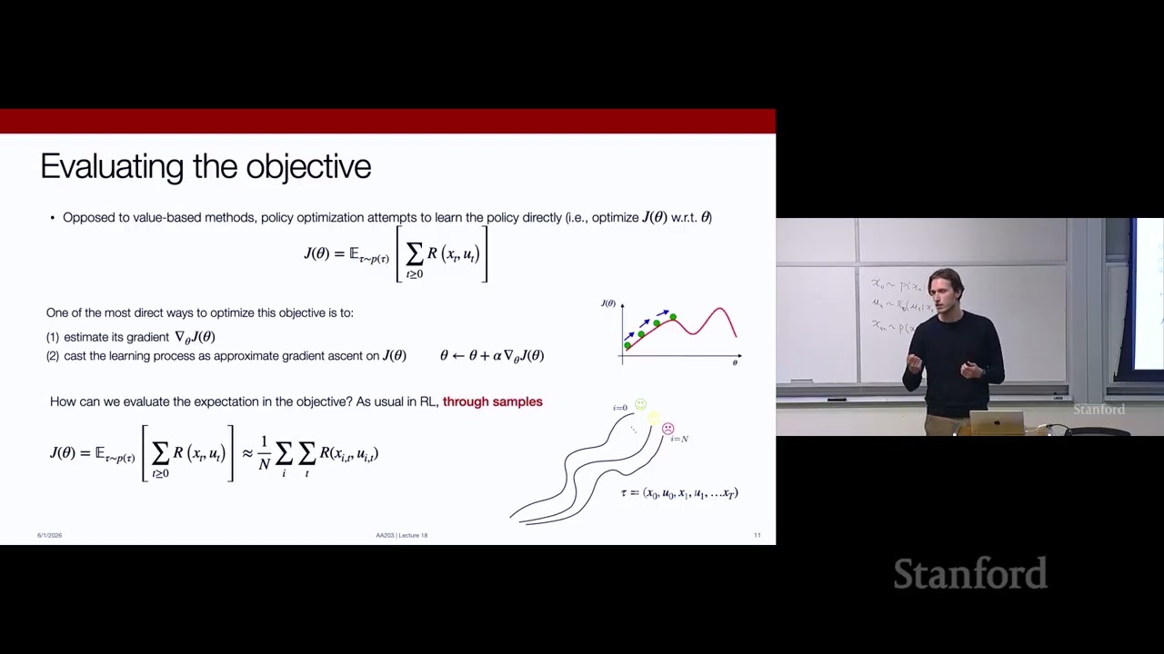
In value-based reinforcement learning, the optimal policy was sought indirectly through fixed-point iterations on value functions (such as Bellman updates), backed by convergence guarantees showing that iterating $Q$-values leads to optimal behavior. Policy optimization tackles the optimization problem directly. Treating $J(\theta)$ as an unconstrained numerical optimization objective suggests using gradient ascent to iteratively hill-climb parameter space:
Evaluating and optimizing $J(\theta)$ presents an immediate challenge: the expectation is taken over $p_\theta(\tau)$, which depends on unknown environment transition dynamics $p(x_{t+1} \mid x_t, u_t)$. Dr. Gammelli emphasizes that the standard model-free remedy is empirical sampling through environment interaction:
- When an analytical expectation cannot be evaluated because system dynamics are unknown, the expectation is approximated using empirical rollouts.
- By executing policy $\pi_\theta$ across $N$ independent trajectories in the environment, the expectation of total trajectory return is estimated by the empirical sample mean:
[09:07](https://www.youtube.com/watch?v=a1g9U_5zO54&t=547s) Formulating the Policy Gradient Objective
To implement gradient ascent, one must compute the analytical gradient of the performance metric with respect to the policy parameters, $\nabla_\theta J(\theta)$. For concise notation, Dr. Gammelli defines $r(\tau)$ as the scalar cumulative reward collected across an entire trajectory $\tau$:
$$r(\tau) = \sum_{t=1}^T r(x_t, u_t)$$
With this shorthand, the objective function is written as an explicit integral over all possible trajectories:
At face value, this formulation is not directly computable because $\nabla_\theta p_\theta(\tau)$ depends on the probability distribution of trajectories, which embeds unknown transition dynamics and the initial state distribution. To turn this into an actionable, sample-based estimator that can be evaluated strictly from interaction data, Dr. Gammelli sets up the next mathematical step: applying the score function / likelihood-ratio identity to massage $\nabla_\theta p_\theta(\tau)$ into an expectation over $p_\theta(\tau)$ that eliminates the unknown transition dynamics entirely.
[12:13](https://www.youtube.com/watch?v=a1g9U_5zO54&t=733s) The Log-Derivative Trick and Eliminating Environment Dynamics
To convert the gradient of the expected reward into a computable expression, Dr. Daniele Gammelli applies the standard log-derivative identity (often called the likelihood ratio trick or REINFORCE trick). Recognizing that the gradient of the logarithm of a function is simply the gradient of the function divided by the function itself—$\nabla \log f = \frac{\nabla f}{f}$—one can rewrite the gradient of the trajectory probability as $\nabla p(\tau) = p(\tau) \nabla \log p(\tau)$. Substituting this identity into the policy gradient integral yields:
While expressing the gradient as an expectation under the trajectory distribution is a critical step forward—because expectations can be approximated by sampling rollouts from the environment—it is not yet immediately actionable. The term $\nabla_\theta \log p_\theta(\tau)$ still appears to depend on the full trajectory distribution, which includes unknown environment transition dynamics.
```mermaid
flowchart TD
accTitle: Factorization and Gradient of Trajectory Distribution
accDescr: Diagram showing how log trajectory probability splits into components and how taking the gradient eliminates the unknown environment dynamics.
subgraph Decomp ["Trajectory Log-Probability Decomposition"]
Init["Initial State: log p(x₀)"]
Dyn["Dynamics: ∑ log p(xₜ₊₁ | xₜ, uₜ)"]
Pol["Policy: ∑ log π_θ(uₜ | xₜ)"]
end
Init -->|"∇_θ (no θ dependency)"| Zero1["Drops out (0)"]
Dyn -->|"∇_θ (no θ dependency)"| Zero2["Drops out (0)"]
Pol -->|"∇_θ (explicit θ)"| Keep["∑ ∇_θ log π_θ(uₜ | xₜ)"]
```
To resolve this, the lecture revisits the factorized definition of the trajectory distribution: the probability of a rollout $\tau = (x_0, u_0, \dots, x_T)$ is the initial state distribution $p(x_0)$ multiplied by the product over time of the policy probabilities $\pi_\theta(u_t \mid x_t)$ and the environment transition dynamics $p(x_{t+1} \mid x_t, u_t)$. Taking the natural logarithm turns these products into sums:
When taking the gradient with respect to the policy parameters $\theta$, a crucial cancellation occurs: neither the initial state distribution $\log p(x_0)$ nor the transition dynamics $\log p(x_{t+1} \mid x_t, u_t)$ depend on $\theta$. Consequently, their gradients evaluate to zero and vanish entirely from the equation. The only term that survives is the sum of the gradients of the log-policy:
Because the policy is an object designed and parameterized by the practitioner—such as a Gaussian distribution over continuous actions $u_t$ where $\theta$ specifies the mean and variance, or a categorical distribution over discrete actions—the quantity $\log \pi_\theta(u_t \mid x_t)$ is fully known and analytically differentiable. Plugging this back into the expectation gives the complete analytical form of the policy gradient:
[17:18](https://www.youtube.com/watch?v=a1g9U_5zO54&t=1038s) The REINFORCE Algorithm: From Expectation to Empirical Rollouts
With every term inside the expectation fully defined, computing the policy gradient in practice reduces to Monte Carlo approximation. Just as the overall objective was approximated by drawing trajectories, the policy gradient is approximated using an empirical mean over $N$ sampled rollouts collected by executing the current policy $\pi_\theta$ in the environment:
This mathematical foundation forms the basis of REINFORCE, the classic policy optimization algorithm. Taking a bird's-eye view of the algorithm reveals three foundational building blocks that mirror the lecture's general reinforcement learning skeleton:
1. **Sampling:** Generating rollouts by deploying the policy $\pi_\theta$ directly into the environment.
2. **Return Estimation:** Evaluating trajectory returns through pure Monte Carlo estimation by summing up observed rewards across each rollout episode.
3. **Policy Improvement:** Taking a gradient ascent step in parameter space, $\theta \leftarrow \theta + \alpha \widehat{\nabla}_\theta J(\theta)$, using the empirical gradient estimate.
Dr. Gammelli emphasizes that these three steps constitute a single iteration of an inner loop. They are wrapped in an outer loop where the updated parameters $\theta_{\text{new}}$ produce an improved policy, which in turn collects fresh rollout data to re-estimate the gradient, progressively improving performance over training.
[20:52](https://www.youtube.com/watch?v=a1g9U_5zO54&t=1252s) Policy Gradient as Weighted Maximum Likelihood and Trial-and-Error Intuition
To ground the algebra in physical intuition, Dr. Gammelli compares the policy gradient formula to behavior cloning via Maximum Likelihood Estimation (MLE). In standard imitation learning or behavior cloning, one possesses an offline dataset of state-action tuples demonstrations from an expert. The goal is to maximize the likelihood of the expert's actions:
Under pure MLE, taking a gradient step uniformly increases the probability of every action present in the dataset. In sharp contrast, the policy gradient is essentially a "weighted version of the gradient that you would get from maximum likelihood estimation," where the weighting factor is precisely the cumulative trajectory reward $R(\tau)$.
```mermaid
flowchart LR
accTitle: Comparison of Behavior Cloning and Policy Gradient
accDescr: Flowchart contrasting how Maximum Likelihood updates all demonstrations equally while Policy Gradient weights updates by trajectory rewards.
subgraph MLE ["Maximum Likelihood / Behavior Cloning"]
direction TB
BCData["Demonstrations (x, u)"] --> BCGrad["∇_θ log π_θ(u | x)"]
BCGrad --> BCUpdate["Uniformly increases probability of all actions"]
end
subgraph PG ["Policy Gradient (REINFORCE)"]
direction TB
PGRoll["Rollouts τ ~ π_θ"] --> PGGrad["∑ ∇_θ log π_θ(uₜ | xₜ) · R(τ)"]
PGGrad --> PGUpdate["Increases probability scaled by trajectory return R(τ)"]
end
```
The consequence of this reward-weighting is the mathematical formalization of trial and error:
- When the agent samples rollouts across the environment landscape, some trajectories yield high returns while others perform poorly.
- Gradient ascent updates the parameters $\theta$ such that actions along high-reward trajectories receive positive weight, allocating more probability mass to those paths.
- Actions that yield lower or negative returns receive little to no positive update (or get suppressed), making poor behaviors increasingly improbable over time.
- Geometrically, if one envisions trajectories as paths with a certain width representing allocated probability mass, policy gradient widens the paths of successful trajectories while thinning out the bad ones.
A student asks whether this approach is also why people use imitation learning when they "don't have an explicit formulation of the reward." Dr. Gammelli confirms that this is indeed a primary motivation: when specifying a scalar reward function is challenging, imitation learning provides an alternative path by directly mimicking demonstrations, whereas reinforcement learning relies on scalar performance feedback to guide trial-and-error optimization.
[026:09] High Variance in Policy Gradients
Connecting back to earlier discussions on behavior cloning and "reinforcement via supervised learning" methods—where returns could be used to reweight loss functions or filter demonstrations—the instructor emphasizes the core philosophy of policy optimization: parameterizing the policy $\pi_\theta$, formulating RL as an optimization problem over parameters $\theta$, and running gradient ascent using the derived analytical policy gradient.
While the intuitive formulation derived from the log-derivative trick makes conceptual sense, it suffers from a fatal practical flaw: the empirical gradient estimator exhibits extremely high variance. Because learning follows this sample-based gradient estimate, high variance produces an unstable learning signal, leading to poor performance, slow convergence, and volatile training curves. Consequently, the vast majority of policy optimization research focuses on designing techniques to reduce the variance of gradient estimators.
```mermaid
flowchart TD
accTitle: Policy Gradient Variance Problem
accDescr: Flowchart illustrating how sample-based estimation leads to high variance and unstable training.
subgraph SG1["Policy Optimization Core"]
A["Parameterize Policy: π_θ"] --> B["Cast RL as Optimization"]
B --> C["Gradient Ascent via Policy Gradient"]
end
subgraph SG2["The Core Bottleneck"]
C --> D["Sample-Based Estimator"]
D --> E["Extremely High Variance"]
E --> F["Unstable Learning & Slow Convergence"]
end
```
[028:17] Intuition: The Impact of Uncentered Returns
To build intuition for why the variance is so severe, consider an illustrative example where the x-axis represents the space of trajectories and a Gaussian curve represents the distribution over trajectories induced by policy $\pi$. Suppose an agent samples three distinct trajectories:
- Trajectory 1: Positive return
- Trajectory 2: Positive return
- Trajectory 3: Negative return
Under standard policy gradient ascent, the updates push parameter space to make positive trajectories more likely and negative trajectories less likely.
However, if an arbitrary positive constant is added to all three returns—preserving identical relative gaps between them—the raw numerical values all become positive. Because every sampled trajectory now has a positive return, the standard policy gradient step attempts to increase the probability mass across all of them (even the worst one), leading to a much more dispersed update. Because the true gradient expectation is approximated from small sample batches, shifting absolute returns causes the resulting gradient direction to fluctuate wildly.
Responding to a student question regarding whether continuous dense rewards decrease gradient variance compared to sparse goal rewards (e.g., getting 5 points only upon reaching a goal versus receiving proximity-based feedback), the instructor confirms that denser reward signals generally improve learning propagation. This improvement stems not only from variance reduction but also from easing temporal credit assignment across the trajectory.
The first variance reduction technique is an intuitive structural adjustment rooted in physical causality. In the original derivation, the policy gradient weights the score function $\nabla_\theta \log \pi_\theta(a_t \mid s_t)$ by the total trajectory return $\sum_{t'=1}^T r_{t'}$.
However, an action taken at time step $t$ cannot retroactively affect rewards obtained at previous time steps $t' < t$. Weighting $\nabla_\theta \log \pi_\theta(a_t \mid s_t)$ by historical rewards introduces unnecessary noise:
- The formulation is modified to sum only future rewards, replacing the total trajectory return with the "reward-to-go": $\sum_{t'=t}^T r_{t'}$.
- Summing fewer reward terms naturally dampens variance, because each omitted term is a random variable dependent on stochastic transitions $p(s_{t+1} \mid s_t, a_t)$ and stochastic actions $a \sim \pi_\theta(\cdot \mid s)$.
- Dropping pre-$t$ terms directly reduces estimator variance without altering the expectation, providing an immediate, measurable performance improvement.
[035:44] Strategy 2: Baselines and Unbiasedness
The second core strategy introduces a baseline $b$ subtracted directly from the trajectory return:
The goal of baseline subtraction is centering the returns:
- Actions leading to trajectories that perform *better than average* ($R(\tau) - b > 0$) have their likelihood increased.
- Actions resulting in returns that are *worse than average* ($R(\tau) - b < 0$) have their likelihood decreased.
A crucial sanity check is verifying whether subtracting an arbitrary baseline $b$ introduces bias into the gradient estimator. The instructor highlights that the expected value of the baseline term evaluates to zero:
$$\mathbb{E}_{\tau \sim p_\theta(\tau)} \left[ \nabla_\theta \log p_\theta(\tau) \cdot b \right] = \int p_\theta(\tau) \nabla_\theta \log p_\theta(\tau) \, b \, d\tau$$
Applying the log-derivative identity in reverse ($p_\theta(\tau) \nabla_\theta \log p_\theta(\tau) = \nabla_\theta p_\theta(\tau)$):
$$\int \nabla_\theta p_\theta(\tau) \, b \, d\tau = b \nabla_\theta \int p_\theta(\tau) \, d\tau = b \nabla_\theta (1) = 0$$
Because the integral of the probability distribution over all trajectories is identically 1, its gradient with respect to $\theta$ is zero. Thus, subtracting a baseline leaves the gradient estimator completely unbiased in expectation while drastically lowering sample variance.
[039:06] Proving That Constant Baselines Yield Unbiased Estimators
```mermaid
flowchart LR
accTitle: Baseline Unbiasedness Derivation
accDescr: Derivation steps showing why subtracting a baseline constant yields zero expected change.
subgraph S1["Expectation"]
A["E[ b · ∇ log p(τ) ]"]
end
subgraph S2["Log-Derivative Trick"]
B["∫ b · p(τ) · ∇ log p(τ) dτ"] --> C["b · ∇ ∫ p(τ) dτ"]
end
subgraph S3["Zero Gradient"]
D["b · ∇(1) = 0"]
end
A --> B
C --> D
```
Dr. Daniele Gammelli turns to proving mathematically why introducing a baseline $b$ does not destroy the unbiased nature of the policy gradient estimator. Expanding the expectation of the baseline term $\mathbb{E}[b \nabla_\theta \log p_\theta(\tau)]$ through the integral definition gives:
$$\int b \, p_\theta(\tau) \nabla_\theta \log p_\theta(\tau) \, d\tau$$
Applying the log-derivative identity in reverse, $p_\theta(\tau) \nabla_\theta \log p_\theta(\tau)$ reduces directly to $\nabla_\theta p_\theta(\tau)$. Because $b$ is a constant with respect to trajectory rollouts, it factors cleanly out of the integral alongside the gradient operator $\nabla_\theta$. The expression simplifies to:
$$b \nabla_\theta \int p_\theta(\tau) \, d\tau$$
Because $p_\theta(\tau)$ is a valid probability density function over all trajectories $\tau$, its total integral over trajectory space identically equals $1$. The gradient of the scalar constant $1$ is identically zero ($\nabla_\theta (1) = 0$), so the entire subtracted baseline expectation vanishes: $b \cdot 0 = 0$.
This result provides a significant algorithmic advantage: the baseline recenters trajectory returns without shifting the expected value of the gradient estimator. Subtracting a baseline provides variance reduction "basically for free" without introducing bias. Because the purpose is centering returns, a widely used and practical baseline choice is simply setting $b$ to the average return evaluated across the batch of $N$ trajectories:
In practical implementations, this variance reduction directly alters empirical training curves. Even on relatively simple environments, lower-variance gradient estimators accelerate training and improve sample efficiency. More critically, high variance can cause optimization to diverge or plateau, meaning an effective baseline often represents the boundary between an algorithm converging to a high-performing policy versus failing entirely.
[043:17] On-Policy Nature, Continuous Actions, and Value vs. Policy Trade-offs
```mermaid
flowchart TD
accTitle: Comparison of Policy Optimization and Value-Based Methods
accDescr: Architectural trade-offs contrasting Policy Gradient and Value-Based RL algorithms.
subgraph PG["Policy Optimization (Policy Gradients)"]
direction TB
PG1["Direct objective ascent: ∇_θ J(θ)"]
PG2["Native continuous/discrete action distributions"]
PG3["Strictly on-policy: requires current rollouts"]
end
subgraph VB["Value-Based Methods (e.g., Q-Learning)"]
direction TB
VB1["Indirect fixed-point iteration: Bellman optimality"]
VB2["Argmax over actions: non-trivial if continuous"]
VB3["Naturally off-policy: reuses past experience"]
end
```
Stepping back to analyze policy optimization in context, Dr. Gammelli highlights its classification as an on-policy formulation. Because the empirical gradient $\nabla_\theta J(\theta)$ is evaluated using trajectory distributions induced specifically by the current parameter vector $\theta$, every update step renders previous rollouts obsolete. The moment $\theta$ is updated, new trajectories must be collected from the environment using $\pi_\theta$.
The lecture examines two primary advantages of policy gradients alongside their primary drawback:
- **Continuous Action Spaces (Pro):** Policy gradient methods handle continuous action spaces natively. The policy $\pi_\theta(u_t \mid x_t)$ can be explicitly modeled as a parameterized probability distribution, such as a Gaussian distribution with mean and covariance networks, and optimized using the same mathematical framework used for discrete categorical distributions. In value-based methods (like Q-learning), actions are chosen by solving an implicit maximization:
$$\pi(x_t) = \arg\max_{u} Q(x_t, u)$$
While trivial when searching over a small, discrete set of candidate actions, computing an $\arg\max$ over a continuous, high-dimensional control manifold requires solving an embedded optimization problem at every decision step.
- **Direct Objective Optimization (Pro):** Policy optimization directly performs hill climbing on the true reinforcement learning objective: the expected discounted sum of rewards over time. In contrast, value-based approaches solve an intermediate objective using fixed-point schemes derived from the Bellman optimality equations. A student asks what is meant by stopping Q-learning "halfway." Dr. Gammelli clarifies that in gradient ascent, termination before full convergence still yields monotonic improvements toward local maxima with a clear sense of progress. In Q-learning's iterative fixed-point evaluation, intermediate policy iterates lack a guaranteed partial ordering of performance before convergence.
- **Sample Inefficiency (Con):** The strictly on-policy nature of vanilla policy gradients forces the agent to discard past transitions and collect entirely new batches of rollouts after each policy step. This demands millions of environment interactions, making sample inefficiency their most severe operational bottleneck compared to off-policy, replay-buffer-driven methods.
[050:20] Moving Toward Actor-Critic: Mitigating Rollout Variance via Value Functions
The limitations of sample-based trajectory estimation motivate actor-critic architectures, which blend the direct parameter optimization of policy gradients with the predictive machinery of value-based methods. Returning to the policy gradient expression:
The inner sum represents the "reward-to-go"—the accumulated reward from the current time step $t$ through trajectory termination $T$. Dr. Gammelli explains that this empirical reward-to-go is the primary source of variance in the estimator. Because the environment and policy are stochastic, taking identical actions from identical states can produce radically divergent downstream rollouts due to compounding transition and sampling noise.
Using a single rollout's realized return as a proxy for the expected future reward provides only an empirical sample from a broad distribution. Actor-critic methods resolve this limitation: rather than relying on noisy empirical trajectory rollouts to approximate future returns, they train a second function approximator—a critic—to fit and estimate the true expected reward-to-go directly.
[52:56](https://www.youtube.com/watch?v=a1g9U_5zO54&t=3176s) Actor-Critic Architectures: Replacing Sampled Returns with Parametric Value Approximators
Dr. Daniele Gammelli turns to a fundamental problem in pure policy gradient methods: evaluating the reward-to-go using empirical trajectory rollouts introduces massive variance into the gradient estimates. To address this, he asks whether a parametric function can be deployed to directly estimate the ground-truth expectation of interest. This core intuition motivates the class of **actor-critic methods**, which maintain two distinct parametric objects:
1. **The Actor ($\pi_\theta$):** The parameterized policy that dictates control actions and whose parameters $\theta$ are updated via gradient ascent.
2. **The Critic:** A value-approximating function parameterized by $\phi$ that learns to predict the expected reward-to-go, drawing directly on the value function approximation techniques introduced earlier in the course.
By substituting the noisy sample-based empirical return with a learned parametric estimator of the expected value function, the estimator's variance is significantly damped—under the crucial operational assumption that the critic can be fitted accurately. Consequently, instead of scaling the score function $\nabla_\theta \log \pi_\theta(u_t \mid x_t)$ by the raw sampled trajectory return, policy optimization scales it by a learned critic evaluation parameterized by $\phi$.
```mermaid
flowchart LR
accTitle: Actor Critic Variance Reduction Flow
accDescr: Flow diagram showing how the actor policy produces actions while the critic value function evaluates states to reduce policy gradient variance.
subgraph ActorBlock["Actor"]
direction TB
PI["Policy π_θ(u|x)"]
ACT["Action u_t"]
PI --> ACT
end
subgraph CriticBlock["Critic"]
direction TB
VAL["Value Estimator V_φ or Q_φ"]
ADV["Advantage / Evaluated Return"]
VAL --> ADV
end
ACT -->|"Interacts with Environment"| CriticBlock
ADV -->|"Low-Variance Gradient"| PI
```
---
[55:20](https://www.youtube.com/watch?v=a1g9U_5zO54&t=3320s) Incorporating Baselines and Deriving the Advantage Function
Having replaced empirical returns with a fitted Q-function, Dr. Gammelli explores whether this framework can be merged with baseline subtraction to drive variance down even further. Drawing on the principle that baselines serve to center returns around an average reference point, he proposes subtracting a state-dependent baseline $b(x_t)$ defined as the expectation of the Q-function over the policy's control distribution:
Dr. Gammelli highlights a conceptual link that often trips students up: the expected action-value function under the current policy is mathematically identical to the state-value function itself:
To build intuition, he contrasts discrete Gridworld transitions across two perspectives:
- **The action-value function $Q^\pi(x_t, u_t)$:** Incorporates one extra piece of explicit information—it commits rigidly to a chosen control $u_t$ at current time $t$, and only averages over the policy's distribution from timestep $t+1$ onward.
- **The state-value function $V^\pi(x_t)$:** Averages over *all* candidate actions that could be selected at time $t$ according to the control distribution $\pi(u_t \mid x_t)$, alongside all subsequent steps.
This quantity is universally termed the **advantage function**. Rather than blindly reinforcing an action based on whether its absolute return is positive, the advantage measures how much better taking specific action $u_t$ is relative to the policy's expected average performance from state $x_t$. Updates guided by $\nabla_\theta \log \pi_\theta(u_t \mid x_t) A(x_t, u_t)$ naturally increase the probability of actions that outperform the local average while depressing the probability of actions that underperform it.
- Action values $Q^\pi(x_t, u_t)$ commit deterministically to action $u_t$ at step $t$.
- State values $V^\pi(x_t)$ marginalize out control choices at time $t$ across policy distribution $\pi_\theta(u_t \mid x_t)$.
- The difference $A(x_t, u_t) = Q(x_t, u_t) - V(x_t)$ centers gradient updates around zero, cutting variance while preserving an unbiased direction in expectation.
---
[01:03:02](https://www.youtube.com/watch?v=a1g9U_5zO54&t=3782s) Student Discussion: Critic Independence, Stochastic Policies, and Pre-Training
The class prompts an engaging exchange on how the actor and critic interact in practice:
A student asks whether the critic is essentially decoupled from the actor—whether one could replace the actor with an entirely new policy while keeping the same critic. Dr. Gammelli clarifies that while actor and critic are distinct mathematical networks, their parameters are inherently coupled during training: the critic estimates the value of trajectories generated by the *current* actor $\pi_\theta$. Because the training data and future rollouts reflect the actor's behavior, the critic cannot simply be treated as an agnostic, standalone representation of the environment.
When asked how an average action is computed under the policy, Dr. Gammelli explains that the policy is a probability distribution over actions:
- In continuous action spaces, $\pi_\theta(u_t \mid x_t)$ is frequently parameterized as a Gaussian distribution.
- In discrete action spaces (such as the four cardinal directions in a Gridworld), $\pi_\theta(u_t \mid x_t)$ is a categorical distribution over discrete options.
In both settings, taking the average action corresponds to taking the formal expectation over this distribution.
Another student inquires whether a pre-trained critic could be used to warm-start training and avoid learning from scratch. Dr. Gammelli offers two perspectives:
- **Theoretically grounded answer:** Strictly speaking, no. Value functions are defined with respect to the specific control policy being evaluated ($V^\pi$), so a mismatch between policies violates the policy evaluation equations.
- **Pragmatic practical answer:** If a pre-trained critic provides an approximation that remains broadly aligned with the gradient descent landscape, it can provide useful inductive bias or stabilization in applied workflows.
Addressing how the critic parameters $\phi$ are updated in practice, Dr. Gammelli points ahead to the upcoming slides: the critic is trained via function approximation strategies directly analogous to fitted Q-learning and temporal difference methods covered in prior lectures. Actor-critic architectures combine the strengths of both worlds: policy gradients optimize control decisions directly, while value-based estimators stabilize the learning signal.
[01:07:12](https://www.youtube.com/watch?v=a1g9U_5zO54&t=4032s) Synthesizing Fitted Q-Learning, REINFORCE, and Actor-Critic
To understand how policy optimization connects to previous concepts, Dr. Gammelli contrasts fitted Q-learning, the REINFORCE algorithm, and actor-critic architectures. In fitted Q-learning, an agent executes its current policy in the environment to gather trajectory rollouts, then fits a parameterized value function $Q_\phi$ to target values—derived either via Monte Carlo returns or temporal-difference (TD) targets—by minimizing a mean squared regression error. Actor-critic methods borrow this exact value-fitting mechanism. Trajectories are sampled from the environment, and a parametric critic model (which can be a state-value function $V$, an action-value function $Q$, or an advantage function $A$) is fit to targets using identical regression techniques.
The divergence occurs in how the learned function is utilized. Fitted Q-learning uses the estimated Q-function to implicitly specify the policy (typically through an $\arg\max$ operation over actions). In contrast, actor-critic methods operate like REINFORCE: the critic's output is plugged directly into an analytical policy gradient expression, and the gradient is evaluated to take an explicit gradient step in the policy's parameter space $\theta$. The actor-critic paradigm is essentially the structural fusion of these two classical lineages, taking the parametric value fitting from Q-learning and combining it with the parametric policy updates of REINFORCE.
```mermaid
flowchart TD
accTitle: Actor-Critic Algorithmic Architecture
accDescr: Diagram illustrating the closed-loop execution and learning updates between actor and critic.
subgraph Rollout ["Environment Rollout"]
P["Current Policy π_θ"] -->|"Sample Actions"| ENV["Environment"]
ENV -->|"Collect Trajectories (s, a, r, s')"| DATA["Rollout Buffer"]
end
subgraph Critic_Branch ["Critic Update (Fitted Value Learning)"]
DATA -->|"Fit Regression Target (MC or TD)"| C["Critic V_ϕ / Q_ϕ"]
C -->|"Compute Target Error"| MIN["Minimize Regression Loss"]
end
subgraph Actor_Branch ["Actor Update (Policy Gradient)"]
C -->|"Estimated Value / Advantage"| PG["Policy Gradient: ∇_θ J(θ)"]
DATA -->|"log π_θ(a|s)"| PG
PG -->|"Gradient Ascent Step"| P
end
```
---
[01:09:13](https://www.youtube.com/watch?v=a1g9U_5zO54&t=4153s) Trade-offs in Function Estimation and Advantage Actor-Critic (A2C)
A fundamental design decision in critic design is deciding which target function to approximate. There is no single correct answer, as differing formulations present distinct computational and statistical trade-offs:
- **State-value function $V(s)$**: Only takes states as inputs, simplifying function approximation because the network does not need to resolve action-space interactions.
- **Action-value function $Q(s, a)$ and Advantage function $A(s, a)$**: Require mapping joint state-control spaces $(s, a)$ to scalars, increasing dimensionality and sample complexity.
In the popular Advantage Actor-Critic (A2C) algorithm, the policy gradient is weighted by the advantage function $A(s, a) = Q(s, a) - V(s)$. Naively estimating this would require parameterizing and training two separate neural networks—one for $Q(s, a)$ and one for $V(s)$. To circumvent this computational overhead, A2C relies on a single-step Bellman approximation for the Q-function:
$$Q(s_t, a_t) \approx r(s_t, a_t) + \gamma V(s_{t+1})$$
Substituting this into the advantage definition yields:
$$A(s_t, a_t) \approx r(s_t, a_t) + \gamma V(s_{t+1}) - V(s_t)$$
This formulation reparameterizes the advantage purely in terms of the state-value function $V(s)$ and instantaneous rewards. As a result, the critic only needs to learn a single state-dependent value network $V_\phi(s)$, yet the actor receives an explicit advantage signal to drive low-variance policy updates.
---
[01:12:19](https://www.youtube.com/watch?v=a1g9U_5zO54&t=4339s) Fitting the Critic: Monte Carlo vs. Temporal-Difference Targets
To address a student question regarding the practical mechanics of critic estimation, Dr. Gammelli highlights that critic training is identical to value function approximation in standard value-based algorithms. Practitioners generally select between two regression regimes:
- **Monte Carlo Estimation**: The agent rolls out complete trajectories to observe actual cumulative returns $G_t = \sum_{k=t}^T \gamma^{k-t} r_k$. A supervised dataset of state-return pairs $(s_t, G_t)$ is curated, and the critic parameters $\phi$ are optimized via gradient descent on the mean squared error $\frac{1}{2} (V_\phi(s_t) - G_t)^2$. This yields unbiased targets but suffers from high variance.
- **Temporal-Difference (TD) Learning**: Instead of waiting for full trajectory completion, the algorithm constructs one-step bootstrap targets $y_t = r_t + \gamma V_\phi(s_{t+1})$. A dataset of tuples $(s_t, y_t)$ is formed to fit $V_\phi(s_t)$ via regression. This approach dramatically reduces target variance and can run in non-terminating tasks, at the expense of introducing bias through bootstrapping.
---
[01:13:46](https://www.youtube.com/watch?v=a1g9U_5zO54&t=4426s) Case Study: AlphaGo as Policy Gradient with Baseline and Search
Dr. Gammelli pivots to a case study on DeepMind's AlphaGo to demonstrate how modern RL milestones map cleanly onto the day's lecture concepts:
- **Policy Network**: Maps current board configurations (states) to probability distributions over legal moves (discrete action space).
- **Value Network**: Parametric state-value function mapping board configurations to scalar values estimating win probabilities.
- **Self-Play Mechanism**: Trained via self-play where policy models compete against historical versions of themselves in simulation, generating games to formulate policy gradient updates.
- **REINFORCE with Baseline**: The parameter update follows an empirical policy gradient:
$$\Delta \theta \propto \frac{1}{m} \sum_{i=1}^m \nabla_\theta \log \pi_\theta(a_i | s_i) \left(z_i - V(s_i)\right)$$
Here, $z_i \in \{+1, -1\}$ denotes the terminal game outcome (return), and $V(s_i)$ acts as a state-dependent baseline for variance reduction.
- **Search Integration**: Crucially, inference does not simply draw raw samples from the categorical policy distribution $\pi_\theta$. Instead, the policy network guides a Monte Carlo Tree Search (MCTS) process to evaluate future board trajectories before making moves.
---
[01:18:00](https://www.youtube.com/watch?v=a1g9U_5zO54&t=4680s) Q&A: Optimality Guarantees, Self-Play, and Future Lectures
The lecture concludes with an interactive discussion on empirical RL results and system dynamics:
- **Absence of Theoretical Guarantees**: A student asks whether AlphaGo's policy came with guarantees of optimality or if it was simply tuned until human grandmasters could no longer win. Dr. Gammelli clarifies that deep reinforcement learning lacks theoretical proofs of convergence or optimality guarantees. Beating the world champion served as empirical validation of performance rather than a mathematical guarantee.
- **Evolution Beyond Behavioral Cloning**: Another student asks about human expert data. In early AlphaGo iterations, training was warm-started using supervised behavioral cloning on expert games before RL fine-tuning. However, subsequent iterations (such as AlphaGo Zero) demonstrated that pretraining on human games proved detrimental to peak performance; learning purely from scratch via self-play unlocked novel superhuman strategies.
- **Adversarial Non-Stationarity in Self-Play**: In response to a query about whether self-play policies risk getting stuck playing against stale parameters, Dr. Gammelli explains that periodically updating the opponent ensures an escalating ladder of proficiency. This iterative adversarial loop forces the learning agent to hill-climb against progressively stronger versions of itself.
Dr. Gammelli closes by announcing that the policy optimization unit will conclude on Wednesday, after which the class will transition to model-based reinforcement learning.
## Notable quotes
> [02:05](https://www.youtube.com/watch?v=a1g9U_5zO54&t=125s) Concretely, this could be like the `env.reset()` method in our Gym environment, for example. — Dr. Daniele Gammelli
> [05:36](https://www.youtube.com/watch?v=a1g9U_5zO54&t=336s) When an analytical expectation cannot be evaluated because system dynamics are unknown, the expectation is approximated using empirical rollouts. — Dr. Daniele Gammelli
> [20:52](https://www.youtube.com/watch?v=a1g9U_5zO54&t=1252s) weighted version of the gradient that you would get from maximum likelihood estimation — Dr. Daniele Gammelli
> [35:44](https://www.youtube.com/watch?v=a1g9U_5zO54&t=2144s) Because the integral of the probability distribution over all trajectories is identically 1, its gradient with respect to θ is zero. — Dr. Daniele Gammelli
> [39:06](https://www.youtube.com/watch?v=a1g9U_5zO54&t=2346s) Subtracting a baseline provides variance reduction 'basically for free' without introducing bias. — Dr. Daniele Gammelli
> [43:17](https://www.youtube.com/watch?v=a1g9U_5zO54&t=2597s) The moment θ is updated, new trajectories must be collected from the environment using π_θ. — Dr. Daniele Gammelli
> [50:20](https://www.youtube.com/watch?v=a1g9U_5zO54&t=3020s) Rather than relying on noisy empirical trajectory rollouts to approximate future returns, they train a second function approximator—a critic—to fit and estimate the true expected reward-to-go directly. — Dr. Daniele Gammelli
> [55:20](https://www.youtube.com/watch?v=a1g9U_5zO54&t=3320s) Rather than blindly reinforcing an action based on whether its absolute return is positive, the advantage measures how much better taking specific action u_t is relative to the policy's expected average performance from state x_t. — Dr. Daniele Gammelli
> [01:03:02](https://www.youtube.com/watch?v=a1g9U_5zO54&t=3782s) Actor-critic architectures combine the strengths of both worlds: policy gradients optimize control decisions directly, while value-based estimators stabilize the learning signal. — Dr. Daniele Gammelli
> [01:07:12](https://www.youtube.com/watch?v=a1g9U_5zO54&t=4032s) The actor-critic paradigm is essentially the structural fusion of these two classical lineages, taking the parametric value fitting from Q-learning and combining it with the parametric policy updates of REINFORCE. — Dr. Daniele Gammelli
> [01:18:00](https://www.youtube.com/watch?v=a1g9U_5zO54&t=4680s) Beating the world champion served as empirical validation of performance rather than a mathematical guarantee. — Dr. Daniele Gammelli
## Mentioned
Dr. Daniele Gammelli, Prof. Marco Pavone, Stanford University, Italian Institute of Artificial Intelligence (AI4I), DeepMind, AlphaGo, AlphaGo Zero, Principles of Robot Autonomy, Gym, REINFORCE, Advantage Actor-Critic (A2C), Monte Carlo Tree Search (MCTS), NVIDIA, Technical University of Denmark (DTU)
Read the companion textbook, Principles of Robot Autonomy, free online: https://porabook.com
To learn more about enrolling in AA203 Optimal and Learning-Based Control, visit: https://online.stanford.edu/courses/aa203-optimal-and-learning-based-control
Follow along with the course schedule and syllabus: https://stanfordasl.github.io/aa203/sp2526/
Bio: Dr. Daniele Gammelli is the Research Director of the Machine Intelligence for Robot Autonomy Laboratory at the Italian Institute of Artificial Intelligence (AI4I), and a Researcher in the Department of Aeronautics and Astronautics at Stanford University. Since 2022, he has been a Research Fellow at the Center for Aerospace Autonomy Research (CAESAR) at Stanford and, until 2025, at the Center for Automotive Research at Stanford (CARS). He received his Ph.D. in Machine Learning and Mathematical Optimization from the Technical University of Denmark (DTU) in 2022, where his doctoral thesis was nominated for the DTU Best Thesis of the Year Award and the DTU Young Researcher Award. Dr. Gammelli’s research focuses on developing the algorithmic foundations and system-level methodologies that enable AI-powered autonomous systems to operate safely, efficiently, and reliably in high-stakes environments, with an emphasis on aerospace autonomy and next-generation mobility systems.
Instructors:
Prof. Marco Pavone, Associate Professor of Aeronautics and Astronautics, Director of Autonomous Vehicle Research at NVIDIA
Dr. Daniele Gammelli, Research Director at the Italian Institute of Artificial Intelligence (AI4I), Researcher at the Department of Aeronautics and Astronautics, Stanford University
Full playlist: https://www.youtube.com/playlist?list=PLa9dmHsLK9dg
Dr. Daniele Gammelli presents policy optimization as a direct, model-free reinforcement learning approach that optimizes explicit control policies via gradient ascent, eliminating unknown environment dynamics through the log-derivative trick while mitigating severe gradient variance using baselines and actor-critic architectures.
Policy Gradients and the REINFORCE Derivation (12:13)
Dr. Gammelli outlines policy optimization as a direct parameter search maximizing expected cumulative return \(J(\theta)\), contrasting it with value-based fixed-point iteration. Because environment transition dynamics \(p(x_{t+1} \mid x_t, u_t)\) are unknown, the objective's analytical gradient cannot be evaluated directly across all trajectories. Applying the log-derivative identity \(\nabla p(\tau) = p(\tau) \nabla \log p(\tau)\) reformulates the gradient as an expectation under sampled trajectory rollouts: \(\mathbb{E}_{\tau \sim p_\theta}[\nabla_\theta \log p_\theta(\tau) r(\tau)]\).
Expanding the log trajectory distribution separates the initial state and transition probabilities from the parameterized policy \(\sum_t \log \pi_\theta(u_t \mid x_t)\). Because environment dynamics do not depend on \(\theta\), their gradients evaluate to zero and drop out entirely, leaving only the differentiable policy. This derivation underpins the REINFORCE algorithm, which alternates between sampling empirical rollouts, calculating Monte Carlo returns, and stepping along the gradient. Dr. Gammelli frames this as reward-weighted maximum likelihood estimation: parameter updates widen the probability density over high-reward trajectories while suppressing suboptimal paths.
Variance Reduction via Causality and Baselines
Despite its mathematical elegance, sample-based policy gradient estimation suffers from extreme variance that destabilizes training and slows convergence. For instance, if arbitrary positive constants shift trajectory returns without altering relative differences, gradient ascent uniformly increases the likelihood of all sampled paths. To stabilize optimization without introducing bias, Dr. Gammelli presents two core variance reduction techniques.
First, enforcing physical causality replaces total trajectory return with the reward-to-go \(\sum_{t'=t}^T r_{t'}\). Because decisions at step \(t\) cannot retroactively influence earlier rewards, dropping past terms eliminates extraneous stochastic noise while preserving expected values. Second, subtracting a baseline \(b\) centers returns around a reference threshold. Dr. Gammelli proves that because the trajectory probability distribution integrates to 1, its gradient is identically zero: \(\mathbb{E}[b \nabla_\theta \log p_\theta(\tau)] = b \nabla_\theta(1) = 0\). Subtracting a baseline, such as batch-averaged return, leaves the gradient estimator strictly unbiased while significantly reducing variance.
Actor-Critic Architectures and Advantage Estimation (52:56)
To address the compounding variance of empirical rollouts across long horizons, actor-critic architectures replace noisy Monte Carlo return samples with a learned parametric critic \(V_\phi\) or \(Q_\phi\). Subtracting a state-dependent baseline \(b(x_t) = V(x_t) = \mathbb{E}_{u}[Q(x_t, u)]\) from the action-value function yields the advantage function \(A(x_t, u_t) = Q(x_t, u_t) - V(x_t)\). This formulation scales policy gradients by how much a specific action outperforms the expected local baseline rather than reinforcing absolute returns.
In implementations such as Advantage Actor-Critic (A2C), approximating the Q-function with a single-step Bellman target \(r(x_t, u_t) + \gamma V(x_{t+1})\) allows the critic to estimate only the state-value network \(V_\phi(x)\). Dr. Gammelli notes that critics can be trained via Monte Carlo returns or temporal-difference (TD) bootstrapping, where TD targets lower variance at the expense of introducing bias. While the actor and critic are maintained as separate networks, Gammelli notes they remain coupled during training because the critic evaluates rollouts drawn specifically from the current actor's distribution.
Implementation Trade-offs and Modern Deployment
Dr. Gammelli evaluates key trade-offs between policy optimization and value-based methods. Policy gradients handle continuous control natively by parameterizing continuous distributions, avoiding the challenging continuous \(\arg\max\) operations required by Q-learning. Furthermore, policy gradients climb the true cumulative reward objective directly, ensuring monotonic local improvements. However, vanilla policy gradients are strictly on-policy, requiring newly collected rollouts after every parameter update and demanding millions of environment interactions.
These principles are illustrated through DeepMind's AlphaGo, which integrated a policy network, a value network baseline, and Monte Carlo Tree Search (MCTS) trained via self-play policy gradients. Dr. Gammelli notes that deep reinforcement learning lacks formal convergence or optimality proofs, relying instead on empirical validation. Moreover, while early AlphaGo models initialized weights using behavioral cloning on human games, later iterations like AlphaGo Zero demonstrated that training from scratch through adversarial self-play eliminated human bias and unlocked superhuman strategies.
Dr. Gammelli concludes that while deep policy optimization lacks theoretical optimality guarantees and suffers from sample inefficiency, combining direct policy gradients with causality, baseline subtraction, and critic-based advantage estimation provides a robust foundation for high-dimensional control before transitioning to model-based methods.
Source quotes
[2:05] Dr. Daniele Gammelli: Concretely, this could be like the `env.reset()` method in our Gym environment, for example.
[5:36] Dr. Daniele Gammelli: When an analytical expectation cannot be evaluated because system dynamics are unknown, the expectation is approximated using empirical rollouts.
[20:52] Dr. Daniele Gammelli: weighted version of the gradient that you would get from maximum likelihood estimation
[35:44] Dr. Daniele Gammelli: Because the integral of the probability distribution over all trajectories is identically 1, its gradient with respect to θ is zero.
[39:06] Dr. Daniele Gammelli: Subtracting a baseline provides variance reduction 'basically for free' without introducing bias.
[43:17] Dr. Daniele Gammelli: The moment θ is updated, new trajectories must be collected from the environment using π_θ.
[50:20] Dr. Daniele Gammelli: Rather than relying on noisy empirical trajectory rollouts to approximate future returns, they train a second function approximator—a critic—to fit and estimate the true expected reward-to-go directly.
[55:20] Dr. Daniele Gammelli: Rather than blindly reinforcing an action based on whether its absolute return is positive, the advantage measures how much better taking specific action u_t is relative to the policy's expected average performance from state x_t.
[63:02] Dr. Daniele Gammelli: Actor-critic architectures combine the strengths of both worlds: policy gradients optimize control decisions directly, while value-based estimators stabilize the learning signal.
[67:12] Dr. Daniele Gammelli: The actor-critic paradigm is essentially the structural fusion of these two classical lineages, taking the parametric value fitting from Q-learning and combining it with the parametric policy updates of REINFORCE.
[78:00] Dr. Daniele Gammelli: Beating the world champion served as empirical validation of performance rather than a mathematical guarantee.
Original transcript
[0:06] So welcome to the
last week of W23.
[0:10] So from our usual roadmap,
for the last few weeks,
[0:15] we have been in the top right
quadrant of our roadmap,
[0:17] specifically looking at
learning-based methods
[0:19] for optimal control.
[0:21] And over the last
couple of weeks,
[0:23] we've basically been introducing
the reinforcement learning
[0:25] setting, where we are
looking at ways to estimate
[0:28] value functions.
[0:30] Specifically, we introduce Monte
Carlo and temporal difference
[0:33] learning as really fundamental,
model-free learning strategies.
[0:37] And last week, we also looked at
one of the families of methods
[0:41] for model-free reinforcement
learning, namely
[0:43] value-based methods.
[0:46] On the other hand,
today, we switch topics
[0:49] and we complete, if
you wish, and start
[0:51] to discuss the second main
family of methods that
[0:54] belong to the model-free
reinforcement learning family,
[0:56] namely policy optimization.
[0:58] And as we will see today,
in policy optimization,
[1:02] differently from what we
did in value-based methods,
[1:04] whereby the policy is implicitly
defined through the value
[1:08] function itself.
[1:10] In policy
optimization, we'll see
[1:11] how we will be representing
the policy explicitly, namely
[1:14] through parametric
representation of the policy,
[1:16] and then tune or
adjust the parameters
[1:19] of this parametric
representation of the policy
[1:22] to directly maximize the
reinforcement learning
[1:24] objective.
[1:25] But long story
short, today, we'll
[1:27] be looking at policy
optimization methods.
[1:31] Specifically, we'll start
by introducing and defining
[1:35] policy gradients,
which will lead us
[1:38] into the very first
algorithm, which will
[1:40] be the reinforced algorithm.
[1:41] And we'll do some
discussions on the role
[1:45] of variants of these
policy gradient estimators.
[1:48] Then we'll be looking at that
actor critic methods, which
[1:51] are extremely popular
instantiation of policy
[1:54] optimization, and then conclude
with some mention to kind
[1:59] of recent reinforcement learning
algorithms and applications.
[2:05] So let's start
from-- if you recall,
[2:07] at the beginning
of our discussions
[2:09] on reinforcement learning, we
loosely introduced reinforcement
[2:13] learning as a problem,
where we have an agent that
[2:16] interacts with the environment.
[2:18] Through this
interaction, we generate
[2:21] some trajectories style,
which are nothing else
[2:23] than a kind of sequences
of states and controls
[2:25] that we observe over time.
[2:28] And through this, we defined
the formalism for reinforcement
[2:33] learning as a Markov
decision process,
[2:35] whereby we defined a
trajectory distribution
[2:40] p of tau, where p of
tau essentially encodes
[2:43] all the stochasticity that
we have in the environment.
[2:47] Namely, we could
have an initial state
[2:50] x0, which is sampled from a
distribution over x states.
[2:54] Concretely, this could be like
the dot reset method in our gym
[2:57] environment, for example.
[3:00] We have uncertainty that
comes from the policy itself,
[3:03] so we are defining a policy
pi as a distribution over
[3:06] controls given states, and
so this is in itself is also
[3:10] a random process.
[3:12] And then we obviously
discussed also
[3:14] the stochasticity that comes
from the transition function
[3:17] itself, which is a
distribution over next state xt
[3:21] plus 1 given the current
state xt and the control ut.
[3:27] And so by taking all of these
sources of stochasticity
[3:31] and factorizing them, as we've
shown here on this slide,
[3:34] we basically derive the
probability distribution
[3:38] over all possible
trajectories style
[3:41] as this factorized
distribution over here.
[3:47] Why was this important?
[3:48] It was important
because this enabled
[3:50] us to define the reinforcement
learning objective, essentially
[3:53] as a maximization problem,
where we want to basically pick
[3:57] the policy pi that maximizes
a certain objective.
[4:00] And this objective is the sum of
discounted cumulative rewards,
[4:05] but the sum of discounted
cumulative returns
[4:07] is an expectation,
where the expectation is
[4:10] under this trajectory
distribution,
[4:12] so this is basically where we
started a couple of weeks back.
[4:17] How does policy optimization
go for solving this problem?
[4:20] As we were briefly
mentioning before,
[4:22] in policy optimization,
what we do
[4:25] is we essentially
define our policy
[4:28] to be a parametric
policy, pi of theta,
[4:30] with some parameters theta.
[4:32] And therefore, the
reinforcement learning objective
[4:36] and the trajectory
distribution itself
[4:38] can essentially be
written with respect
[4:40] to these parameters theta.
[4:43] So the initial state
distribution and the transition
[4:47] distribution do not
depend on theta directly,
[4:50] but our policy does indeed
inform the evolution
[4:54] of the trajectory.
[4:55] And therefore, what we
want to pick essentially,
[4:58] is the values of
the parameters theta
[5:01] that maximize the RL objective.
[5:05] So long story short, at face
value in a policy optimization,
[5:09] we take the reinforcement
learning objective as it is,
[5:13] and we basically define
it as a optimization
[5:17] problem with respect to the
parameters of our policy.
[5:22] Again, going forward, to
simplify the notation,
[5:24] we will assume that this is
an undiscounted environment,
[5:27] but everything still
holds when we actually
[5:29] account for discounting.
[5:36] So let us start solving
this problem in practice.
[5:41] So we saw how--
[5:44] well, in value-based
methods, if you remember,
[5:46] we were ideally solving
this exact same problem,
[5:50] but we were doing this
in an indirect way
[5:52] because we were doing
essentially fixed point
[5:55] iteration on q values
and value functions.
[5:59] And then we saw that
that convergence--
[6:01] we derived some theory,
or, at least, mentioned
[6:04] some theory for which the
algorithms that we proposed
[6:08] would converge to the
optimal value function
[6:10] and therefore to
the optimal policy.
[6:12] In reinforcement
learning, now we
[6:14] want to solve this explicit
optimization problem.
[6:19] So we know that,
before in this class,
[6:22] we mentioned as a good idea when
we want to solve optimization
[6:28] problems, that gradient
ascent or gradient descent
[6:31] is a good approach for
solving a general class
[6:33] of numerical
optimization problems.
[6:36] Fundamentally, if we were
to approach this problem
[6:39] through gradient
ascent because we
[6:41] want to maximize this
objective function,
[6:44] we would need to
first of all estimate
[6:46] the gradient of the objective
we're interested in,
[6:49] and then basically cast
learning or learning
[6:52] the policy as doing gradient
descent on the objective
[6:55] that we care about.
[6:57] That is, iteratively takes
steps in parameter space,
[7:00] following the direction that is
given to us by this gradient,
[7:04] so pictorially, hill
climbing are RL objective.
[7:12] A first question
here is already we
[7:16] see how our objective
that we wish to optimize
[7:20] is a non-trivial
object because we
[7:22] have this expectation under the
trajectory distribution, which
[7:26] is something which we
don't really know about
[7:28] because the trajectory
distribution, as we said before,
[7:31] has these three sources
of stochasticity,
[7:34] so we can assume that
we know our policy
[7:37] and we can evaluate the
distribution under our policy,
[7:41] but we don't really know
the transition dynamics,
[7:43] for example, because
this is the whole point.
[7:47] So our first question
is, how can we
[7:50] even evaluate this
expectation in the objective?
[7:53] And the answer here
is, by basically
[7:55] leveraging the same tools that
we discussed over and over
[7:59] the last couple of weeks,
which is essentially, sampling.
[8:02] So in reinforcement
learning, whenever
[8:03] we don't know some quantity,
for example, the transition
[8:06] functions, we go around it by
sampling in the environment.
[8:12] What did we mean by sampling?
[8:13] So far, is essentially
taking rollouts
[8:15] and interacting with our
environments over time.
[8:19] So in other words, we
have this objective
[8:22] that we wish to
optimize, which entails
[8:26] computing the expectation under
the trajectory distribution.
[8:29] We don't know how to
compute this expectation,
[8:32] and so we can approximate
it by running our policy n
[8:36] times in the environment and
just taking the empirical mean.
[8:42] So in practice, you
could imagine indeed
[8:44] following n possible
rollouts of our policy.
[8:48] These rollouts will
have some rewards.
[8:50] We will be observing different
quality of these rollouts,
[8:53] and then we simply average
out all of the rewards
[8:56] that we observe over time.
[8:57] And this would be a
valid approximation
[9:00] of this expectation.
[9:07] So we mentioned that we
want to approach this
[9:11] through stochastic gradient
ascent or gradient ascent.
[9:15] The first thing
that we need to do
[9:16] is compute the gradient right.
[9:18] So what we'll do right now is
basically derive the policy
[9:22] gradient and specifically derive
actionable kind of expression
[9:29] of the policy
gradient, and then see
[9:31] how we can use this expression
within working algorithms.
[9:35] Any questions so far?
[9:43] Great.
[9:47] So for compactness,
let us define
[9:50] r of the trajectory tau
as the sum of rewards
[9:54] that we observed in a
specific trajectory,
[9:56] so simply the sum of all the
rewards observed from time 1
[10:00] until time t within
that trajectory tau.
[10:06] So we can use this r tau
to basically rewrite the RL
[10:10] objective that we were
introducing before,
[10:12] so J of theta,
which we introduced
[10:15] before as being the expectation
under the trajectory
[10:18] distribution of
the sum of rewards,
[10:20] we can just write it
as a small r of tau.
[10:23] And by definition
of expectation,
[10:25] we can write this expectation
as the integral of p tau times
[10:30] r tau into tau.
[10:35] So what we said is
what we want to take
[10:38] the gradient of this
objective function
[10:39] and use this to hill climb.
[10:41] So given this
definition or rewriting
[10:44] of the objective J of
theta, the gradient
[10:48] of J of theta with
respect to theta
[10:50] is the integral of the
gradient with respect
[10:53] to theta of p tau times r tau
and the tau, so nothing special
[10:58] here.
[10:59] We rewrote our RL
objective and then
[11:03] we're taking the gradient at
face value of that objective.
[11:11] So here, of course, in--
[11:14] this would not be
actionable because we
[11:16] would like to
evaluate this gradient
[11:18] and basically, take a step in
the direction of that gradient.
[11:21] But the problem here is that
how we define it right now,
[11:25] basically the gradient
depends on unknown dynamics
[11:29] and the initial
state distribution
[11:31] through the probability
of trajectories p tau,
[11:37] so this is still the
object that we don't really
[11:39] know how to compute.
[11:44] So here, essentially, what
we'll be doing in this slide
[11:47] and the next is that
we'll be basically
[11:50] massaging this definition
of the policy gradient
[11:53] until we derive an analytically
tractable and actually
[11:58] computable expression
of that same gradient.
[12:02] So the first thing
that we do is,
[12:04] so we realize that this is the
object that is creating problems
[12:08] for us, and so we
leverage that identity
[12:11] on the right of this slide.
[12:13] Specifically, the identity
whereby the probability, p tau,
[12:18] times the grad log p can
be rewritten as the grad p,
[12:23] essentially.
[12:24] So we know that the grad of
the logarithm of a function
[12:29] can be essentially written as
the gradient of that function,
[12:32] divided by the function itself.
[12:35] And so the two terms
cancel out, and so we
[12:37] get that kind of useful
identity on the right.
[12:41] So specifically, now we
can do this substitution
[12:44] in our expression of
the policy gradient.
[12:47] And what we get is that we get
the integral of the p tau, times
[12:53] the grad log p's, times r tau.
[12:56] Always in the tau, of course.
[12:58] Now, again, we can use the
definition of expectation.
[13:03] And we can basically rewrite
this integral as the expectation
[13:09] under the trajectory
distribution
[13:12] of this part over here.
[13:17] Now, this is not actionable
yet because still we
[13:22] have this expectation.
[13:24] And this term here
is not something
[13:27] we know how to deal with,
but you can probably
[13:30] start to see that we are
somehow on the right track
[13:34] because we know that whenever
we have some quantity that
[13:37] is defined as expectations under
the trajectory distribution,
[13:41] we can just approximate this
expectation through interactions
[13:44] with the environment
and through sampling.
[13:47] So this is one step in
the right direction,
[13:49] but still not
completely actionable
[13:51] because we have this grad log p
in the equation, which is still
[13:54] something we don't know.
[13:59] So let's keep going.
[14:03] So let us recall as from the
previous slide, the definition
[14:09] of the trajectory distribution,
which is basically
[14:11] this factorization
of what for us
[14:13] is the trajectory distribution.
[14:16] If we take the logarithm of
the trajectory distribution,
[14:19] products become sums.
[14:21] Each individual terms
becomes the-- of course,
[14:24] we take the logarithm.
[14:26] And basically, what
we get is the log
[14:28] p's is equal to the sum of
these three terms over here.
[14:33] So the logarithm of the
probability of the initial
[14:36] state, plus the sum over time
of the log pi's, essentially
[14:40] the logarithm of the
distribution induced
[14:43] by our policy, and the log p's.
[14:45] That is the transition dynamics.
[14:49] So we just substitute this in
into our equation of the policy
[14:54] gradient, and we get this
object over here, where--
[15:02] yes, so we are taking
the gradient with respect
[15:04] to theta of this
entire term here,
[15:08] which we derived as the
logarithm of the probability
[15:11] distribution over trajectories,
multiplied by the sum of rewards
[15:15] in that trajectory.
[15:18] Now, of course, notice
that since we're
[15:20] taking the gradient
with respect to theta,
[15:24] the first and the
third term here
[15:26] don't depend on theta
directly, so they don't
[15:29] contribute to our gradient.
[15:33] And notice that the
only term that remains
[15:36] is actually something
that we know
[15:38] how to compute because the
policy is an object we define.
[15:44] For example, the
policy for us might
[15:48] be a Gaussian over a
one-dimensional continuous
[15:52] action, so we could
have our u of t.
[15:56] And so our policy
pi of ut given xt
[16:02] might be a Gaussian, where
the parameters theta might
[16:06] represent maybe the mean and
the variance of that Gaussian.
[16:09] And so basically, the log
pi's are completely specified,
[16:16] and so we can actually
evaluate them.
[16:20] And so this means that if we
take that expression over there
[16:23] and just rewrite it
compactly over here,
[16:28] where the only thing that
changes that we re-expanded
[16:30] our terms small r of tau.
[16:35] We see that we get an expression
of the policy gradient, which
[16:39] is something where
first of all, everything
[16:41] inside this
expectation is known,
[16:44] so this is just
the sum of rewards
[16:45] that we observe according
to some trajectories tau.
[16:49] This is the sum of the log pi's
according to our policy, which,
[16:53] again, is something we
know how to compute,
[16:55] and so everything inside
this expectation is known.
[17:01] Do these steps make sense
or any questions until now?
[17:13] So we said that everything
inside this expectation
[17:16] is known.
[17:18] How do we evaluate
this in practice?
[17:20] We use the same trick.
[17:21] So we have this
expectation under
[17:23] the trajectory distribution.
[17:25] We know that we can approximate
this as the empirical mean
[17:29] by basically sampling n
rollouts in our environment.
[17:33] We did this before
for the objective,
[17:35] so we can do exactly the same
with the policy gradient, which
[17:40] basically means that we can now
completely evaluate the policy
[17:44] gradient that we're interested
in by taking n rollouts
[17:50] or trajectories, basically
tau's in the environment,
[17:55] computing this quantity for
all of these trajectories,
[17:58] and taking the mean.
[18:00] And this would be a
valid approximation
[18:02] of the policy gradient.
[18:17] And so basically,
if this is clear
[18:21] through this derivation
of the policy gradient,
[18:26] this leads us directly
into, if you wish,
[18:28] the very first
policy optimization
[18:31] algorithms that we will see in
this class, which is also known
[18:35] as the reinforced algorithm.
[18:38] So as you can probably
imagine, the derivations
[18:43] that we derived so far basically
give us an actionable strategy,
[18:47] because now what we can do
is something along the lines
[18:49] of these three steps over here.
[18:52] So we will be sampling
n trajectories
[18:55] from the environment by
basically just letting
[18:57] our policy interact with
the environment itself.
[19:01] Through these
trajectories, we can now
[19:03] always evaluate these gradient,
or the policy gradient,
[19:06] or, at least, approximate it.
[19:08] And once we have this estimate
of the policy gradient,
[19:12] we can take a step in
the parameter space,
[19:14] according to this gradient,
to improve basically
[19:19] the quality of our
parameters pi theta
[19:22] that represent our policy pi.
[19:29] So taking the bird's eye view
on this reinforce algorithm,
[19:32] according to our usual
skeleton, kind of we
[19:35] have our usual three
components, whereby
[19:38] we are generating
samples by interacting
[19:40] with the environment.
[19:42] We are estimating our
return through Monte Carlo,
[19:46] because we're basically running
our policy in the environment
[19:49] and explicitly summing
up all of the rewards
[19:52] that we observe at the
end of our episode,
[19:55] and then we're using those
estimates of the returns
[19:58] to improve the
policy, namely taking
[20:01] a step in parameter space.
[20:08] Of course, this is,
if you wish, one step
[20:14] of an inner loop,
whereby we would then
[20:16] have to repeat this over time.
[20:18] So here, we're taking
one gradient step,
[20:20] but then you can
imagine that we have
[20:23] outer for loop that is kind
of wrapping these three
[20:27] steps, where we repeat this
process because now we will have
[20:30] an improved policy with some
new parameters theta, which will
[20:33] collect new experience, and
we'll use this experience
[20:36] to re-estimate the gradient
and keep iterating over time.
[20:52] But let's stop for
a second and try
[20:55] to build some intuition into
what policy gradient is actually
[20:59] doing under the
hood and indeed, get
[21:01] some intuition behind the math,
which I think is always useful.
[21:06] So we did all of those
kind of algebraic steps
[21:11] to basically derive this
estimator for the policy
[21:15] gradient.
[21:19] We explained before how
the log pies essentially
[21:23] represent the log
probabilities of the action
[21:32] according to our policy.
[21:33] And we saw before how this
could be represented either
[21:36] in the continuous space,
exactly as we were doing here
[21:39] on the slide, but
this is equally
[21:41] holds if we're looking at
a discrete action space,
[21:45] whereby namely, the
policy will be expressing
[21:48] a categorical distribution
over a finite set of actions
[21:52] that we could pick.
[21:54] And so this is basically
the term that we derived.
[21:58] But it's useful to compare
it with the expression
[22:01] of the gradient
that we would when
[22:03] we try to perform
maximum likelihood,
[22:05] or if you wish, kind of
behavior cloning for us
[22:08] for the purpose of control.
[22:11] So remember the setting
of behavior cloning.
[22:13] In behavior cloning, we
have some demonstrations
[22:15] of an expert doing something
and executing a task, which
[22:19] for us, namely means data sets
of tuples of states and action
[22:24] pairs, which basically are
examples of this mapping
[22:28] that we wish to approximate.
[22:33] In maximum likelihood
estimation or behavior cloning,
[22:36] what we wanted to
do is, we wanted
[22:37] to maximize the
probability of the actions
[22:41] that we observed from our
expert given the state.
[22:46] And so formally, the gradient
in the maximum likelihood case
[22:50] would essentially be
comprised of this term, where
[22:54] we are trying to maximize the
probability of the actions
[22:59] in our data set because
this would essentially
[23:02] mean be equivalent
to approximating
[23:05] the behavior of the expert.
[23:10] If you compare this
equation of the gradient
[23:15] to what we just derived
for the policy gradient,
[23:18] you see that this is
essentially a weighted version
[23:22] of the gradient that you would
get from maximum likelihood
[23:26] estimation, where the weight is
specifically the sum of rewards
[23:30] in that trajectory.
[23:33] So what does this mean?
[23:35] Is that in behavior
cloning, we taking a step
[23:38] in the direction of the
gradient, essentially
[23:41] means updating the probability
of all the actions in my data
[23:45] set.
[23:47] In policy gradient, we are
updating the probability
[23:51] of the actions according
to their performance
[23:54] in those rollouts,
so those actions that
[23:57] led to higher reward are more
updated in my policy gradient
[24:03] term, and so we're
updating that probability,
[24:05] if that makes sense.
[24:10] Is this clear?
[24:12] Does that make sense?
[24:25] Indeed, and so the
policy gradient
[24:26] is a weighted version of the
maximum likelihood estimation
[24:29] gradient.
[24:31] So again, to hammer
down this idea,
[24:37] if we take a step in the
direction of the policy
[24:40] gradient, what we're
doing is that we're
[24:42] changing the parameters
theta such that trajectories
[24:45] with high reward have
higher probability.
[24:49] And so you could imagine if we
have this fictitious landscape
[24:54] of rollouts, where
the width of the lines
[25:00] here represents the
probability mass
[25:02] that my policy is allocating
to those trajectories.
[25:06] Then here what we
want is we want
[25:08] the good trajectories
to be more likely
[25:12] than the bad trajectories.
[25:13] And so in a way, policy
gradient really formalizes
[25:17] this idea of learning
by trial and error,
[25:19] because we are running out
kind of getting rollouts
[25:24] in of the policy
in the environment,
[25:26] so we're trying out
different strategies.
[25:28] And then through basically
updates in parameter space,
[25:33] we are learning what
is more effective
[25:37] and making it more
likely, and we're
[25:39] learning what is less effective
and making it less likely.
[25:53] And there's a lot of
imitation learning context.
[25:56] We could use this
approach because we
[25:58] don't have an explicit
formulation of the reward.
[26:01] Is that kind of why or?
[26:03] I would say, so, yes.
[26:05] For example, you might not
have an explicit measure
[26:07] of the reward.
[26:09] I mean, you could construct
it and then maybe reweight
[26:12] your behavior cloning
loss, for example,
[26:15] so this is something
that if you recall,
[26:18] we did discuss towards the
end of the behavioral cloning
[26:20] class, where we looked at--
[26:22] So we refer to them
as reinforcement
[26:25] via supervised learning
methods, where we did
[26:28] have a notion of
reward, and maybe we
[26:30] use that to filter the
demonstrations or whatnot.
[26:33] But so at face value, yes,
this is the reason why.
[26:42] And so I would say, this is
probably the most fundamental
[26:49] idea for this lecture.
[26:51] So we started saying,
we want to approach
[26:56] the reinforcement
learning problem
[26:57] from a slightly different angle.
[26:58] That is one of
policy optimization,
[27:01] so we parameterize
our policy, and then
[27:03] we cast reinforcement
learning as an optimization
[27:07] problem with respect to these
parameters of the policy.
[27:11] And to do this, we
do gradient ascent,
[27:13] and so everything
that we've done so far
[27:14] is derive the expression
of the gradient.
[27:18] So of course, this is not it.
[27:21] There is much more to policy
optimization in the sense
[27:24] that what we discussed
so far is great,
[27:26] and from an
intuitive standpoint,
[27:29] it also makes a lot of sense,
at least, to me personally.
[27:33] But I would say that if
you look at this gradient,
[27:36] there are some clear
limitations, and I would say,
[27:39] the main one is the fact
that this gradient, so
[27:42] our estimate of the gradient,
has extremely high variance.
[27:46] And so this is an
extremely, if you wish,
[27:49] unstable learning
signal to follow.
[27:53] But so let us now
spend a few minutes
[27:57] on this problem of high
variance of the policy gradient.
[28:00] And so we'll do now is,
we'll first briefly build
[28:05] some intuition to why this high
variance might be happening,
[28:08] and then we'll look
at two strategies
[28:10] for reducing the variance
of the policy gradient.
[28:17] So consider this, again,
kind of fictitious example
[28:20] here on the slide.
[28:21] Specifically, here
we are visualizing,
[28:25] if you wish, on the x-axis
the space of trajectories,
[28:29] so all possible
trajectories that we may
[28:32] follow according to our policy.
[28:36] And this Gaussian here
is basically represents
[28:40] a distribution over trajectories
induced by our policy pi.
[28:47] Now, say that we basically run
our policy in the environment
[28:52] and we observe
three trajectories,
[28:55] and these three trajectories
have some associated return.
[28:58] So we have these
three trajectories,
[29:00] we sum up all of the rewards,
and we obtain this three
[29:04] specific performances.
[29:08] Now, out of these
three, two of them
[29:10] were positive in this direction
and one of them was negative.
[29:15] Now, from everything that we've
said so far on policy gradient,
[29:21] well, we would expect
to policy gradient
[29:24] to do is that if we then
use these trajectories,
[29:27] estimate the gradient and
take a step in the parameter
[29:30] space, what we're doing is that
we're making this behavior more
[29:34] likely than this behavior
here because this
[29:36] is exactly what we've
been discussing so far.
[29:39] And this is actually
what would happen.
[29:42] But now let's suppose that
we take those same three
[29:46] trajectories and simply add
the same positive constant
[29:52] to the returns to get
these three new values.
[29:56] So the relative gap
is always the same,
[29:59] but what changes is the
kind of absolute numbers
[30:01] of those rewards.
[30:04] The catch here is that if we now
would do the exact same thing,
[30:07] that is policy gradient on these
trajectories, what we would get
[30:10] is something slightly
more dispersed.
[30:13] So because this is also a
positive number, in this case,
[30:17] policy gradient
will still try to--
[30:21] well, it will try to of
course, give more likelihood
[30:23] to the better ones,
but it will still
[30:25] try to cover this
trajectory over here.
[30:30] And so, of course, this is, if
you wish, an extreme example,
[30:34] but the main idea that
I'm trying to convey here
[30:36] is that because
we are estimating
[30:39] the true value of
the policy gradient
[30:42] through samples, depending on
the samples that we observe,
[30:46] the policy gradient can vary
also quite substantially.
[30:49] And so this is
exactly what we mean
[30:52] that the estimator that we came
up with of the policy gradient
[30:55] has a high variance.
[30:59] Why do we care about this?
[31:00] Is because in practice,
if our estimator
[31:03] of the gradient that we follow
for learning has high variance,
[31:06] this will essentially
lead to worse performance,
[31:09] slower convergence, and
potentially more unstable
[31:13] training curves, essentially.
[31:16] So within this
framing, I would say
[31:20] that a lot, if not the
majority of the research
[31:24] in policy optimization,
essentially revolves
[31:27] around finding ways to lower the
variance of these estimators,
[31:32] and so different algorithms
essentially boil down
[31:35] to instantiating the policy
gradient in different ways.
[31:44] Any questions on this?
[31:47] Yeah.
[31:49] So rewards can be discrete
or can be continuous.
[31:52] And it's just like a more
clear gradient decrease
[31:57] the variance of
the policy gradient
[31:59] is another interpretation?
[32:01] Sorry.
[32:02] Compared goal point let
say, and you reach the goal,
[32:07] you get 5 points,
versus you get points
[32:10] based on proximity to the goal,
so just continuous signal.
[32:13] Just supplying a
continuous reward signal
[32:16] decrease the variance?
[32:18] Yes, I would say that
in general, the more
[32:21] dense your reward
is, the better it
[32:25] is for propagating that learning
throughout the algorithm,
[32:28] in general.
[32:30] Now, it's not only because
of the variance of the policy
[32:32] gradient, but I would
say, in general,
[32:34] also for credit assignment.
[32:37] So if basically,
it encodes learning
[32:41] to be more granular throughout
your entire trajectory,
[32:44] if that makes sense, but yes,
your intuition is correct.
[32:53] So let's look at a
couple of strategies
[32:56] to reduce the variance
of policy gradients.
[32:59] So the first one, I would say,
is more than a simple trick
[33:04] than an actual strategy.
[33:06] In the sense that
if we look back
[33:07] at what we were doing to
define the policy gradient,
[33:11] we essentially defined it as,
of course, the empirical mean,
[33:14] because we want to
approximate the expectations.
[33:16] We have this first term,
which is the log pi's.
[33:18] Great, something we can compute.
[33:20] And we were weighting
the log pi's
[33:22] by the sum of rewards throughout
the entire trajectory.
[33:26] Now, if you look a little bit
more closely into what this is
[33:31] doing, is that what it may
happen that for time t prime,
[33:36] greater than t, the log pi's
of this t prime would still be
[33:42] weighted by the sum of all
the t's before t prime,
[33:46] which is something
counterintuitive,
[33:48] because basically the policy
at time t prime cannot really
[33:53] affect the reward for the
time steps before that action.
[33:58] And so this is what I mean by
causality here on the slide.
[34:02] And so the first trick
essentially entails leveraging
[34:05] this intuition for the fact that
actions at time t prime cannot
[34:10] affect the rewards
that happen before it,
[34:12] and simply encode this into
how we are defining the policy
[34:16] gradient.
[34:19] So right now, here, I'm just
taking out this summation
[34:22] to make it more explicit.
[34:25] But so rather than
summing from t
[34:27] equals 1, what we
would be doing here
[34:29] is summing from t prime
equals t, specifically.
[34:36] So this makes sense intuitively,
but why does this lower
[34:40] the variance?
[34:40] So first of all,
of course, we're
[34:42] not including a lot of terms on
which the action doesn't really
[34:45] have any influence on.
[34:47] And then also, I would
say quite intuitively,
[34:52] we are summing less terms
in our policy gradient.
[34:55] Less terms of the reward.
[34:58] And remember that the
reward is essentially
[35:00] something that depends on a
number of stochastic elements
[35:04] throughout the trajectory.
[35:06] So again, throughout
the trajectory,
[35:08] we will be sampling repeatedly
from our policy, which
[35:11] is indeed something stochastic.
[35:13] We'll be sampling repeatedly
from the transition
[35:15] function, which is also
something stochastic.
[35:18] And so simply put, here
we're summing less terms,
[35:22] and so there is less variance
associated with this policy
[35:25] gradient, overall.
[35:32] Does this make sense?
[35:33] This is pretty simple
trick, I would say,
[35:35] but it does indeed
measurably improve things.
[35:44] The second strategy,
which I would
[35:46] say is very important for the
space of policy optimization
[35:52] methods, is one of introducing
the concept of baselines.
[35:57] So to understand exactly
what we mean by baseline,
[36:00] let's reconsider the
intuition we were discussing
[36:03] before regarding
policy gradient,
[36:06] when we were saying that
policy gradient makes
[36:08] good behavior more likely.
[36:12] And so, specifically, what
we're discussing is that policy
[36:17] gradient will only
do, quote-unquote,
[36:21] "the right thing,"
if the returns,
[36:24] that is the sum of all the
rewards that we are observing,
[36:28] were centered.
[36:29] So we specifically consider
this counter example
[36:32] on the right, where the relative
difference was the same,
[36:35] but simply those returns
were not centered,
[36:37] and so the policy gradient
was actually doing something
[36:40] that we didn't want it to do.
[36:43] Intuitively, what we
would like to have
[36:44] instead is that we would like
to use some mechanism to center
[36:49] our returns, such that the
policy gradient essentially
[36:53] becomes something whereby the
probability of behavior that
[36:58] is better than average
gets increased,
[37:00] and the probability of behavior
that is worse than average gets
[37:04] decreased.
[37:06] So in other words, we
want to have a mechanism
[37:09] to recenter the returns
from our interactions
[37:12] with the environment.
[37:15] The way we'll do this
is through something
[37:17] that is referred to
as a baseline, here
[37:19] referred to as b, which
is basically a quantity
[37:22] that we are subtracting
to the sum of reward
[37:26] to the return r of tau.
[37:38] So before we get into actionable
ways of using the baseline,
[37:44] kind of a valuable
sanity check here
[37:47] is so we're
introducing something
[37:48] in the policy gradient.
[37:51] We don't want to change the
expectation of the policy
[37:55] gradient because we derived
our equations analytically.
[38:00] And we know that in
expectation, the policy gradient
[38:02] will go to the limit
of infinite samples
[38:06] from our distribution
over trajectories,
[38:09] we'll get the correct object.
[38:11] But now if we subtract
this baseline b,
[38:13] do we still get the
same expectation?
[38:17] Is the estimator still
unbiased, essentially?
[38:21] And so the claim
here as a spoiler
[38:23] is that adding this
baseline does not
[38:25] change the value of
the expected gradient,
[38:28] and so let's look at this
more and more closely.
[38:34] So to understand
this, let's consider
[38:37] the following expectation.
[38:39] So specifically, let's look
at the part of the policy
[38:48] gradient, which only
takes into account
[38:50] the baseline, so the grad log
p is times the baseline p.
[38:55] Again, from the definition
of the expectation,
[38:58] we can rewrite this
as the integral
[39:00] of p tau, times the grad
log p, times the baseline b,
[39:06] so here just the definition
of expectation again.
[39:11] And now we can use the
exact same identity
[39:14] that we used before in the
derivation of the policy
[39:16] gradient, but now in the
reverse direction, if you wish.
[39:20] So we can basically take
the p times grad log p's,
[39:27] which is equal to the
grad p's over here.
[39:33] And so this entails two grad
p's times the baseline b.
[39:39] Now, we can take the
b because this is just
[39:43] a constant out of the integral.
[39:46] We can do the same with
the gradient operator,
[39:49] and so what we get
is the b multiplied
[39:53] by the gradient of the integral
of the probability of tau
[39:57] in the tau.
[39:58] Since the probability
distribution over trajectories
[40:01] is a valid probability
density, we
[40:03] know that the integral
has to be equal to 1.
[40:07] And so what we get is we
get b, times the gradient
[40:10] of a constant,
which is equal to 0.
[40:19] And so this basically
makes the estimate
[40:22] of the gradient with the
additional baseline term still
[40:26] unbiased in expectation
because here,
[40:29] we basically verified
that the expected value
[40:33] of the term that we are
subtracting is equal to 0,
[40:36] and so we're not really
changing the actual expectation
[40:39] of our estimator, which
is something pretty
[40:49] neat because basically
now we have this mechanism
[40:51] through which we can recenter
the returns in our policy
[40:54] gradient, and therefore, reduce
the variance basically for free,
[40:58] because we're not really
losing anything in terms
[41:01] of bias of our estimator.
[41:06] Since what we say is that
the goal here is to center
[41:09] the returns, a pretty
effective and popular choice
[41:14] of the baseline is actually
to define the baseline
[41:16] as the average return.
[41:18] So remember, again,
here we are interacting
[41:21] n times with our environments,
so we have n trajectories tile.
[41:25] For all of these trajectories,
we will have some return,
[41:28] and so we just define
b as the average return
[41:31] over our trajectories.
[41:35] We'll see how this
idea of average returns
[41:38] basically motivates many
popular reinforcement learning
[41:40] algorithms, but for
now, I would say,
[41:43] this is the intuition that
we are trying to capture.
[41:46] So remember what
we're doing here.
[41:50] We are interested in using
policy gradient like algorithms.
[41:55] We recognized that the policy
gradient is a high variance
[41:58] object, and so we want to reduce
this variance through baselines.
[42:02] And here, we basically
showed one way of doing so.
[42:13] Any questions on this?
[42:24] What does it mean in
practice to have a baseline?
[42:26] Again, this is just kind of
a simple example of training
[42:30] curves, but to give you an idea
is that in practice what this
[42:33] would mean is that even for
very simple environments,
[42:36] you would get a
much faster training
[42:42] for the exact same
algorithm when
[42:44] you're just changing the
expression of the policy
[42:46] gradient.
[42:47] So here, we're
basically looking at it
[42:50] from the perspective of
maybe sample efficiency,
[42:52] so you converge faster,
but in some cases
[42:54] this actually makes
the difference
[42:56] between converging or not
converging to a good solution.
[43:01] So basically, this
is what I mean
[43:03] when I say that the quality
of the estimator of the policy
[43:07] gradient actually influences
training quite substantially.
[43:17] So let's take a step back and
think about what we're doing.
[43:23] So everything that
we've done so far today
[43:25] is basically defining
a different way
[43:29] of solving the reinforcement
learning objective.
[43:31] First of all, we express it as a
function of the parameters theta
[43:36] of our policy, we evaluate the
gradient of that objective,
[43:40] we saw how to do it, and we
take a step in parameter space
[43:44] according to this gradient.
[43:46] Now, given basically this
high level structure,
[43:49] if you recall last
week, we were discussing
[43:52] the differences between on
and off policy algorithms.
[43:55] Specifically, we mentioned
that an on policy algorithm
[43:59] is an algorithm that
uses experience collected
[44:03] under the policy that we are
using to explore the environment
[44:07] to improve.
[44:10] Would you say that this is an on
policy or off policy algorithm
[44:14] in this case?
[44:16] Yeah.
[44:17] [INAUDIBLE] are
updating the policy
[44:21] under different
runs of the market?
[44:24] Yeah, exactly.
[44:25] So this is in this
specific framework,
[44:29] as we've have seen so far,
policy gradient algorithms
[44:32] are indeed a
naturally on policy,
[44:35] because the estimate
of the gradient
[44:39] depends on basically,
the rollouts that we
[44:42] did in the environment,
according to the current policy
[44:46] pi theta.
[44:48] The moment we update
the policy, we'll
[44:50] have to collect new
experience in order
[44:52] to re-evaluate the policy
gradient for that policy.
[45:01] Of course, there are extensions
of policy optimization.
[45:04] So the takeaway here is
not policy optimization.
[45:07] Algorithms are on
policy, but there
[45:09] are for the way we
derive it so far,
[45:12] these are indeed on
policy algorithms.
[45:18] And indeed, exactly
as we said, it
[45:20] is on policy because we need
samples from the current policy
[45:24] to estimate the gradient.
[45:27] So let's look a little
bit more closely
[45:29] at a couple of pros and cons
of policy gradient methods.
[45:35] First of all, it's
nice to point out
[45:40] how policy gradient
methods naturally handle
[45:44] continuous action spaces.
[45:46] And this is because
basically, all we have to do
[45:49] is we have to define an
appropriate representation
[45:52] of our policy pi of ut given xt.
[45:55] For example, this
could be a Gaussian,
[45:57] and we parameterize the
parameters of that Gaussian.
[46:00] So same thing if we were to
use a discrete distribution, so
[46:06] a categorical
distribution, we will
[46:08] be essentially able to leverage
the exact same formalism
[46:11] regardless if the action space
is continuous or discrete.
[46:16] On the other hand, in
value-based methods,
[46:19] if you recall, the policy for
us was basically, implicitly
[46:23] defined as an argmax over you
of, for example, a q function.
[46:32] Doing this argmax is obviously
easy in the moment in which this
[46:36] is the action space is
discrete, so we have finite set
[46:40] of values for our actions u.
[46:42] The moment u is a
continuous object, then
[46:45] this in itself is an
optimization problem,
[46:47] so which might or
might not be trivial.
[46:53] Same caveat here.
[46:54] There are, of
course, methods that
[46:56] allow value-based methods to be
applied for continuous action
[47:00] spaces, but at face value,
this is a clear distinction.
[47:08] A second pro is that
by how we derived it,
[47:13] policy optimization
methods directly
[47:16] optimize the objective
we care about,
[47:18] which is the discounted
sum of rewards over time.
[47:21] So we are clearly
differentiating
[47:26] between policy
optimization methods that
[47:28] take the rl objective and
optimize this objective at face
[47:32] value, so we literally
do gradient ascent
[47:34] on that objective.
[47:36] From value-based methods
such as q-learning,
[47:39] which derive a mechanism, for
example, the Bellman optimality
[47:44] equations, to enforce a kind
of a fixed point iteration
[47:49] scheme that at
convergence will also
[47:52] lead to optimizing
that same objective,
[47:55] but for intermediate solutions,
it's not really clear
[47:58] if there is a partial ordering.
[48:00] So for policy
optimization method,
[48:03] since we're doing hill
climbing, if we stop halfway,
[48:07] we probably have a good
estimate of how much we
[48:10] have been improving over time.
[48:12] On the other hand,
with q-learning, we
[48:14] know that we have
guarantees of convergence,
[48:16] but if we stop halfway,
we don't really
[48:18] know how we are with
respect to previous versions
[48:22] of the policies we computed.
[48:28] Yes.
[48:29] Sir, what do you mean by, for
q-learning, to stop halfway?
[48:33] Yes, so in both cases,
remember that we're
[48:36] looking at sequential
iterative algorithms.
[48:39] So here, this is
basically gradient ascent,
[48:41] which we take sequential steps.
[48:43] In q-learning, we are basically
doing fixed point iteration,
[48:47] so we are recursively enforcing
maybe the Bellman optimality
[48:50] equation.
[48:51] In both cases, you might
stop before convergence.
[48:57] In policy optimization
case, I would
[48:59] argue it's pretty clear
to understand progress
[49:02] because you're
maximizing an objective.
[49:05] In q-learning,
it's less clear how
[49:07] to value, to compute,
or evaluate progress
[49:10] in between before you
reach convergence.
[49:19] But I would say,
the bottom line here
[49:21] is that in value-based
learning, we
[49:23] are introducing an intermediate
objective to achieve
[49:27] the same thing, while
in policy optimization,
[49:29] we say we want to optimize the
rl problem and we just do that.
[49:37] The con is that at face value,
at least, the kind of algorithms
[49:41] we just discussed are on policy
compared to, for example,
[49:46] q-learning, which might be prone
to off policy learning as well.
[49:50] And so on policy in this
case can be extremely sample
[49:54] inefficient, whereby
we essentially,
[49:57] mean that we might have to
interact with the environment
[49:59] many, many times before
we actually converge.
[50:08] Any questions so far before we
move on to actor-critic methods?
[50:20] And so let's now look at
actor critic methods, which
[50:25] build, I would say,
quite substantially
[50:29] on all the ideas we
introduced so far,
[50:31] namely the policy gradient.
[50:34] But I would say, at their
core, actor-critic methods
[50:37] try to blend and leverage
the best of both worlds
[50:43] between policy gradient methods
and value-based methods,
[50:47] and we'll see shortly how.
[50:53] So specifically, consider,
again, the policy
[50:56] gradient expression
we just derived,
[50:58] which is, again, the sum.
[51:01] So the average of the
sum of the log pi's,
[51:05] times the sum of the
reward of our trajectory.
[51:09] The sum of rewards from
time t up until capital T,
[51:13] is also referred
to as the reward
[51:15] to go, because
essentially, encodes
[51:17] all of the rewards
that we will be
[51:19] seeing in the future
of our trajectory.
[51:27] And in a way basically,
all of the discussions
[51:31] of the high variance
of the policy
[51:33] gradient that we were doing
before, essentially boil
[51:35] down that to the fact
that this reward to go
[51:42] is indeed the part
whereby we have
[51:46] that is basically contributing
to this high variance
[51:48] because this reward
to go, we only
[51:50] have a limited sample estimate
of what the expected reward
[51:57] to go is.
[51:59] And when we actually sample
from the environment,
[52:02] this might only be kind of a
noisy estimate of the ground
[52:06] truth expectation
we're interested in.
[52:10] Why is this a noisy estimate?
[52:12] Is because, again, as
we were saying before,
[52:14] we are basically
repeatedly sampling
[52:16] from various sources
of noise, and so even
[52:19] if we were to take the exact
same sequence of actions,
[52:22] over time, we might end in
slightly different rollouts
[52:25] in our environment.
[52:30] So I would say,
actor-critic methods
[52:32] are kind of fundamentally
say the following.
[52:37] So rather than estimating
these expected rewards
[52:43] to go through sampling,
whereby sampling
[52:46] basically entails just
evaluating rollouts
[52:48] of our policy and
the environment,
[52:50] why don't we try to estimate the
actual expectation by fitting,
[52:56] for example, a
parametric function,
[53:02] to basically estimate
this ground truth
[53:04] expectation that we care about?
[53:08] And so at a high level,
what actor-critic methods do
[53:12] is that they define two
parametric functions that we
[53:15] are interested in learning.
[53:17] The first one is the actor.
[53:19] Basically, our policy, so
our policy pi of theta.
[53:22] So we have some
parameters theta that we
[53:24] wish to estimate as
we're doing so far,
[53:26] but they also introduce a critic
that is basically a mechanism
[53:30] to estimate more accurately
the expected reward to go
[53:35] that we would like to have.
[53:38] How do we do this?
[53:40] This is basically
everything that we
[53:41] have been doing so far in
the last couple of weeks,
[53:45] which is basically, we want to
estimate the value functions.
[53:50] And so we saw before
already how we can use,
[53:54] for example, parametric
approximations
[53:56] to estimate an approximate
value functions.
[54:01] So very high level, what
actor-critic methods do
[54:06] is that they recognize that
part of this high variance
[54:11] problem that we see
in policy gradients
[54:13] basically is caused by
approximating the reward
[54:19] to go through samples.
[54:21] And so instead of approximating
this reward to go to samples,
[54:25] let's fit a parametric
approximator of the ground truth
[54:30] expectation, which assuming
we are able to do correctly,
[54:34] then this will reduce the
variance of my policy gradient.
[54:39] So putting this together,
instead of multiplying my log
[54:43] pi's by the sample return
as we were doing over there,
[54:48] so our reward to go,
let's replace the reward
[54:51] to go with an estimator
of, for example,
[54:55] a value function with
some parameters phi.
[55:07] Does this make sense?
[55:20] And so if this is clear--
[55:24] so this is a good
idea, so let's just fit
[55:29] a parametric function
to our value functions.
[55:33] Can we combine what we're
doing, so this idea,
[55:37] with the discussion on
baselines that we did before?
[55:41] Well, the answer is yes.
[55:43] So let us try to reduce
even further the variance
[55:46] of our policy gradient
by basically taking
[55:51] our new estimate of the
policy gradient, where
[55:55] we are using our
fitted q function,
[55:58] and let us add the
baseline again.
[56:03] Exactly as we were
saying before,
[56:05] the intuition that we tried
to leverage in the baseline
[56:07] is that we wanted to
center our returns.
[56:11] And so in this case, to center
our value function here,
[56:19] we could pick a state
dependent baseline b of xt.
[56:22] That depends on state xt, which
is basically the expected q
[56:28] function value.
[56:29] So here, we're basically
doing the same thing.
[56:31] We want to center this quantity.
[56:34] How do we center this?
[56:35] Well, we could pick b as the
expected q function, where
[56:39] this expectation is taken under
the distribution over controls
[56:44] ut according to our policy.
[56:53] So even if the exact details
here are slightly unclear,
[57:01] I would say, the main idea
here that we want to take home
[57:05] is that actor-critic
methods introduce
[57:09] an estimate of
the value function
[57:10] to better approximate
the reward to go.
[57:13] This is great.
[57:14] Can we combine this
idea with baselines?
[57:16] Yes, we can do that.
[57:19] We said that with baselines, we
wanted to recenter our reward
[57:23] to go term.
[57:25] We can center this by picking
the baseline in this way,
[57:28] essentially.
[57:37] Now, let's look at this term
a little bit more closely.
[57:42] The expected q function
under our policy
[57:47] is basically nothing else that
the value function itself.
[57:52] So this is something that can
be somewhat confusing at first,
[57:58] but let us try to
look a little bit more
[58:01] closely with an example.
[58:03] So consider a discrete
environment, again, for example
[58:08] our gridworld, where
we can take maybe one
[58:11] of a finite number of actions.
[58:17] So we know that the q
function, in this case,
[58:23] under some policy pi is
basically the expected reward
[58:33] that we expect to have
in state x, taking action
[58:37] ut, and then following the
policy pi for all the time
[58:43] steps that come.
[58:44] So this is the definition that
we had so far of the q function.
[58:51] Where specifically you see
that here we are basically
[58:54] picking the action ut
because the q function
[58:57] is defined over this
tuple, states and controls.
[59:01] How can we connect
the q function
[59:03] with the value function
for that same policy?
[59:09] Is that intuitively,
the value of a state
[59:13] is the average
value that we would
[59:19] get of the future states,
where this average is taken
[59:25] under the probability
distribution that
[59:29] decides which action I'm picking
right now, if that makes sense.
[59:32] So this value function
here is basically
[59:38] averaging out the
future values, according
[59:41] to all the possible controls
that I might pick in that state.
[59:49] Does this make sense?
[59:51] Yeah.
[59:52] So it that-- now we can
cancel the [INAUDIBLE]
[59:54] to where you're looking
over all possible states
[59:58] are up for actions
in the future,
[60:01] and then, like you just
said, averaging them out?
[60:04] Yes, I would say the
intuition is very similar.
[60:06] So maybe one other way to
see this is a temporary.
[60:10] So basically, the only
thing that changes
[60:13] is the one step
reasoning that we're
[60:15] doing, because from
t plus 1 onwards,
[60:19] we're still sampling
from our policy,
[60:21] and so we're averaging out
over all possible things that
[60:23] could happen over our policy.
[60:26] In the one-step, so
from t to t plus 1,
[60:29] the q function is basically
has one information more, which
[60:33] is we are specifying what
control we're taking right now,
[60:37] so we're basically committing
to one specific action.
[60:42] On the other hand,
the value function
[60:44] is a function only of the state.
[60:47] And so what we're
basically saying
[60:49] is that the value of this state,
if we don't know which action
[60:53] we're picking in this
state, will basically
[60:55] depend on the average action
that we're picking in the state,
[60:58] and so the average action is
sampled according to our policy,
[61:07] if that makes sense.
[61:11] So this is just
basically a small detour,
[61:15] but useful to figure out
what we're saying here.
[61:19] So here, we're looking at
introducing the baselines.
[61:23] We mentioned that this was a
reasonable choice of a baseline.
[61:29] We now just saw how the expected
q-function is nothing else
[61:32] than the value function.
[61:35] And so we can then rewrite
the expression of the policy
[61:38] gradient as, again, the
average over n trajectories
[61:42] of the grad log pi's,
multiplied by our critic
[61:46] estimator of the reward to go,
minus the value function, which
[61:50] in this case is the
policy is the baseline.
[61:59] And if you look at this
term a little bit more
[62:02] closely, what this
term is saying
[62:03] is that this is essentially
quantifying how much the action
[62:08] ut is better than the average
action in that same state xt.
[62:14] And so following this
gradient essentially
[62:16] increases the
probability of actions
[62:17] that have returns
better than average
[62:20] and decreases the probability of
the actions that have returned
[62:24] worse than average,
so this is one way
[62:28] of recentering the returns.
[62:32] This quantity is actually
so important in practice
[62:35] that it has its
own name, and it is
[62:37] referred to as the
advantage function
[62:44] because it is as if this
quantity is encoding
[62:47] the advantage of taking
action u with respect
[62:50] to the average action
that I could take.
[63:02] Questions here.
[63:06] Yeah.
[63:07] The critic is like
agnostic of the actor.
[63:12] It's a model of actions
that you can take.
[63:15] It's you could swap out the
actor for a new one [INAUDIBLE],
[63:20] and it would still be
representative of the problem.
[63:22] Is that the right
interpretation?
[63:24] I would say so
functionally, this is just
[63:28] a separate parametric
function, so there
[63:30] are two different objects.
[63:31] Of course, the way we fit the
parameters of the critic, phi
[63:35] in this case,
depend on the policy
[63:37] because you can imagine that
we will be fitting our critic,
[63:44] depending on the experience
that we have in our environment,
[63:47] and this experience is
dictated by the policy.
[63:49] So I would say, this
is not independent,
[63:51] because here,
we're still fitting
[63:52] the value function
of that policy, which
[63:56] for us is the actor.
[63:58] Does that make sense?
[64:00] Yeah.
[64:02] I think a good example on
how policy might give you
[64:05] an average action and
what that might look
[64:07] like for the value function.
[64:10] So remember that
the policy for us
[64:15] is just a distribution
over actions.
[64:16] So in the continuous
case, it could
[64:19] be a Gaussian over a
continuous action ut,
[64:22] or in the discrete
case, it might be say,
[64:26] we have the four cardinal
directions again,
[64:29] and these are our actions.
[64:32] The policy might just be
a categorical distribution
[64:35] over these actions.
[64:38] So what I meant by average
action in all our discussions
[64:43] of value functions that are on
the slide was basically mean,
[64:48] since these are valid
distributions over actions,
[64:53] we could take the expectations
under these distributions,
[64:56] if that makes sense.
[64:59] So this is kind of a
stochastic environment?
[65:05] This would be a
stochastic policy.
[65:07] OK, yeah.
[65:13] Going back to this
question, but even
[65:15] if it will be a different
critic based on the actor,
[65:18] could you use a
pre-trained critic
[65:21] so you don't have to have
it start from scratch
[65:24] at the beginning of
training, or do you always
[65:26] train them together?
[65:30] So I have two answers.
[65:32] One answer is the kind of
theoretically grounded answer.
[65:35] I would say, no, you cannot
do that, because this is--
[65:40] so here, we're estimating
the value function.
[65:42] And remember, the
value function is
[65:43] an object that refers
to a specific policy,
[65:47] so here, we want
to use the value
[65:49] function of the policy
that we're learning,
[65:53] at least, for these algorithms
that we're looking at right now.
[65:56] In practice, as long
as this quantity here
[66:04] is something useful and aligned
for gradient updates, then
[66:11] you might get some benefit in
using a pre-trained critic.
[66:17] What's the one
specific mechanism
[66:19] that you're using to
update the phi parameters?
[66:23] Is it similar to q-learning
or is it something--
[66:25] Yeah, great.
[66:26] It's a great question.
[66:27] It's coming in one or two sides.
[66:30] Short answer is
if you recall what
[66:32] we were doing last week
with fitted q-learning
[66:35] or using function approximators
to estimate the value functions,
[66:40] this is exactly the
same thing, but it's
[66:42] coming in a couple of slides.
[66:50] And so we introduced actor
critic methods as strategies
[66:56] to try to blend the best of
both worlds between policy
[67:01] optimization and value-based
approaches, so let
[67:04] us even just visually look at an
example of a value-based methods
[67:09] in the top left, so
fitted q-learning
[67:12] and the visual version of a
policy optimization algorithm
[67:17] that is reinforce and compare
it with what we're doing here
[67:21] with actor-critic methods.
[67:23] So in fitted q-learning,
if you remember,
[67:25] we were well, of course, running
policy in the environment
[67:28] to collect trajectories.
[67:31] And then we were fitting a
parametric function of our value
[67:36] function q phi in order to
basically solve a regression
[67:41] problem, so we
specifying some targets
[67:43] which could be either the Monte
Carlo targets or the TD target.
[67:47] And then we were trying to
minimize the prediction error
[67:50] from our parametric
approximation and the ground
[67:53] truth target.
[68:00] And this is exactly what we will
find in actor critic methods,
[68:04] so we still run the
policy in our environment
[68:06] to generate trajectories.
[68:08] And here in actor
critic methods,
[68:10] we are fitting either a value
function, or a q function,
[68:13] or advantage function.
[68:15] It will depend.
[68:15] This is a choice,
but we are ideally
[68:17] doing exactly the same thing.
[68:19] So in a way, this is
exactly the same thing
[68:22] we're doing with
fitted q-learning.
[68:23] Here, we're doing
actor-critic methods.
[68:28] At the same time, while
in fitted q-learning,
[68:32] we were using the function to
implicitly define the policy.
[68:39] In actor-critic methods,
we are doing the same thing
[68:42] that we're doing
in the reinforce.
[68:43] That is, we are leveraging
our computations here
[68:47] to define a policy
gradient expression
[68:51] and use this to take a
step in parameter space.
[68:55] So I hope that, at least,
intuitively, you're
[68:59] starting to see how here we're
trying to stitch together
[69:03] different individual components
of different families
[69:06] of algorithms.
[69:13] Now, a question here is--
[69:18] so first of all, we
had many examples
[69:22] of using value functions v
using q functions or advantage
[69:26] functions.
[69:27] What quantity should we estimate
and what are the trade-offs?
[69:31] I would say, in general, there
are no right or wrong answers.
[69:34] I would say,
different algorithms
[69:36] might just have
different implementations
[69:38] of the same underlying idea.
[69:42] But for example, one thing
that you might consider
[69:45] is just the complexity of
the value function estimation
[69:49] problem.
[69:50] So for example,
the value function
[69:53] might be easier because it only
depends on states as the inputs.
[69:57] On the other hand,
if we were to learn
[69:59] a Q function or an
advantage function,
[70:02] we would have to learn a
mapping from states and controls
[70:05] rather than just states.
[70:09] I would say, probably the
most popular implementation
[70:14] of an actor-critic algorithm,
which uses the advantage
[70:19] also refers to as a to z,
or advantage actor-critic
[70:24] is something that has this
specific choice of what
[70:27] we're fitting.
[70:28] So in principle, we want
to use the advantage, which
[70:31] is the q function, minus
the value function v.
[70:36] Of course, what we
want to do is we
[70:38] want to avoid to have
to estimate two objects.
[70:41] We don't want to fit two
separate networks, one for the q
[70:44] function and one for
the value function.
[70:47] And so the trick that
is typically being used
[70:51] is that we can
approximate the Q function
[70:56] as the instantaneous
reward, plus the value
[70:59] function at the next state.
[71:02] And so according to
this approximation, now
[71:06] you can see how the
advantage can be rewritten
[71:10] as a function only of the value
function v of the state value
[71:13] function.
[71:16] And so basically, through this
kind of reparameterization here,
[71:21] this enables us to
basically fit the advantage
[71:24] or use the advantage in our
policy updates, while only
[71:28] having to fit the value
function, if that makes sense.
[71:37] And so indeed, the advantage
actor critic algorithm,
[71:41] or a to z is indeed
something that
[71:45] runs the policy in
the environment,
[71:47] uses those interactions
to fit a value function,
[71:52] uses that value function to
compute the advantage according
[71:56] to this approximation, and then
uses the advantage in the policy
[72:04] gradient expression.
[72:19] So now to answer also to
your colleague's question,
[72:23] so here, we're talking about
estimating different quantities
[72:26] and different value functions.
[72:29] How do we do this?
[72:30] And the main ideas
that we simply
[72:35] leverage exactly what we were
doing in value-based methods
[72:38] with function approximation.
[72:41] Specifically, you could do this
through a Monte Carlo learning.
[72:47] That is, we collect a data
set of state and return pairs,
[72:53] and basically, do
supervised learning
[72:56] on these tuples on these pairs.
[73:02] Or we could use equivalently,
TD learning by similarly,
[73:07] collecting a data set of
state and TD target pairs,
[73:12] and basically solve a
regression problem that
[73:15] fits a value function that
approximates, or minimizes
[73:19] the error with respect
to this target.
[73:28] Does this clarify?
[73:30] Yeah.
[73:38] OK, so now, just
as a brief detour.
[73:46] I wanted to briefly go
through the AlphaGo paper.
[73:52] First of all, to show you
that, this is like 10, 20, 14
[73:59] or something along
those times, but it
[74:04] is one of the biggest successes
of reinforcement learning,
[74:06] arguably.
[74:07] And I definitely invite
you to check out the paper,
[74:09] because I would say that through
everything that we discussed
[74:12] today, we actually can
understand, I would say,
[74:15] the entire paper most likely.
[74:21] And I just want to
highlight a couple of,
[74:23] I think interesting points.
[74:24] So remember, AlphaGo
is basically,
[74:27] this project, where they wanted
to learn through reinforcement
[74:31] learning how to
play Go, which is
[74:35] extremely high dimensional
board game, if you wish.
[74:40] The idea here was to
first of all, define--
[74:46] you already start seeing
a policy network and value
[74:48] network, so here, they
use an actor-critic method
[74:53] for this problem, whereby the
policy is basically something
[74:56] that maps states that is board
configurations to actions, which
[75:02] is a distribution
over a finite amount
[75:06] of next moves in the board.
[75:09] And the value
network is basically
[75:12] a parametric representation of
the state value function, which
[75:16] similarly maps from current
configuration of the board,
[75:20] or the state, to a
scalar number that
[75:24] represents the value of
that board configuration.
[75:28] Now, if we skim to how the
actual algorithm is implemented,
[75:38] so you will see how--
[75:41] So of course, we train
the policy network
[75:43] by policy gradient
reinforcement learning.
[75:49] It was learned
through self-play,
[75:54] so you could imagine having the
policy pitched against itself
[75:59] or previous versions of itself
in a simulated environment.
[76:03] And so the games were replayed
to determine the policy gradient
[76:07] update, which is defined
exactly as we were doing today.
[76:11] Again, the notation slightly
changes, but here, we
[76:15] are basically discussing our--
[76:17] this is the update that
you do in parameter space
[76:20] as the empirical mean 1/m times
a step size alpha of the-- here,
[76:27] we have the grad log pi's, so
the probability distribution
[76:32] over action given state,
times the z here represents
[76:37] the return, so the
return that they observed
[76:40] in the environment, minus the
value function of the state v.
[76:46] And here, they say
that indeed-- so they
[76:48] use the reinforce algorithm
with a baseline v of s, which
[76:53] is basically the value
function as a baseline,
[76:55] and they use this for
variance reduction.
[77:00] Again, I definitely
invite you to check this
[77:03] the details of this
paper, because I
[77:05] would say that vast
majority of the concepts
[77:07] here we did indeed cover today.
[77:10] Is there a reward signal we'll
use at the end of the episode?
[77:14] Yes.
[77:18] Of course, here we glossed over
one of the main contributions,
[77:24] which is the search
element of this approach,
[77:29] meaning in order to
sample from the policy,
[77:32] they weren't just sampling
from a categorical distribution
[77:35] of reaction, but they were
using that distribution
[77:37] to guide an explicit search
process, specifically
[77:40] Monte Carlo tree search.
[77:43] But I would say,
high-level intuitions
[77:45] from the perspective of
the reinforcement learning
[77:48] side of things are exactly
the topics we covered today.
[77:58] Yeah.
[78:00] There was nothing
in the policy they
[78:01] found that guaranteed to be
best, or was it like a human
[78:05] could not beat it?
[78:06] No, so, of course, the moment
you go for deep reinforcement
[78:11] learning algorithms,
there is no theory
[78:13] that can back any of
this in terms of proofs
[78:18] or guarantees of convergence.
[78:21] They were able to beat
the world champion Go,
[78:23] and so they claim this as a good
enough result for this policy.
[78:28] Yeah.
[78:29] Why did they keep the
human-version one [INAUDIBLE]?
[78:36] The full picture here
is that, at the time,
[78:39] the worm started learning
through behavioral cloning,
[78:43] and then they
basically collected
[78:45] data sets of expert
demonstrations
[78:47] and then they fine tuned this
through reinforcement learning.
[78:51] Jump starting this
work, they actually
[78:54] showed that the
behavior cloning part
[78:55] was detrimental to
final performance,
[78:58] and they just learned
everything through self-play.
[79:00] Yeah.
[79:01] Sorry.
[79:02] I know that [INAUDIBLE].
[79:05] You mentioned that like
every 500 iterations,
[79:08] if we updated one that it
was training itself off of,
[79:12] but the parameters have
found worked the best.
[79:14] Do you know if there's a
way that they avoided it,
[79:16] like converging on
some policy just
[79:19] one of those parameters that
the other one was playing with,
[79:22] if that makes sense?
[79:24] I don't think--
[79:24] Or was that part
of my [INAUDIBLE]?
[79:26] [INAUDIBLE] they were doing.
[79:28] I mean, the intuition there is
that you want increasing level
[79:32] of proficiency also for
your kind of adversary,
[79:36] if that makes sense.
[79:39] I'll have to double
check, but I think
[79:41] that just by the fact that you
are updating your adversary
[79:45] and you have this learning loop
that goes around this update,
[79:49] you'll always be incentivized
to find strategies that
[79:53] are better with respect
to your previous version,
[79:56] and so you'll improve hill
climbing in that sense.
[79:59] But maybe they did something
slightly more sophisticated.
[80:02] All right, so finish this
lecture on Wednesday.
[80:06] We'll also start
discussing model based
[80:09] reinforcement learning methods.
[80:10] Thank you.