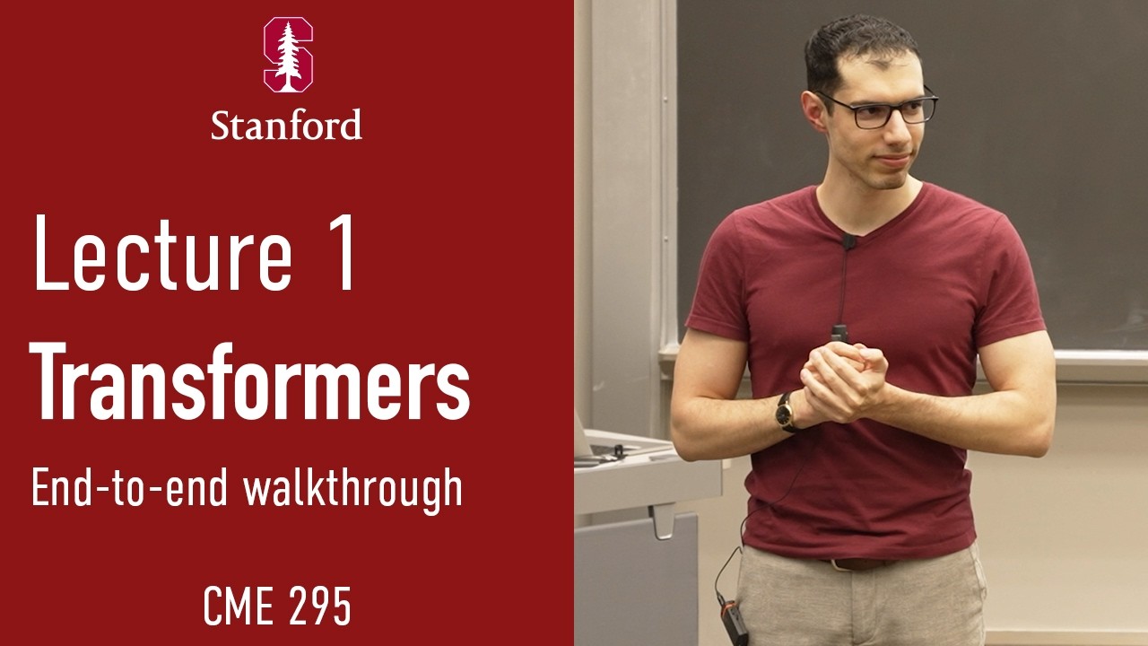
Stanford Instructors Trace Transformer Shift From Chatbots to Agents
Stanford Online
Self-attention eliminates sequential recurrent bottlenecks to enable parallelized web-scale training, while feedforward layers retain the bulk of parameter capacity as models transition to decoder-only autonomous agents.
Stanford CME 295 (Transformers and Large Language Models) returns for its Autumn 2026 edition, incorporating updated topics such as post-training alignment, autonomous coding agents, and non-autoregressive diffusion-based language models. (3:43)
The course identifies the core training bottleneck of RNNs and LSTMs as strictly sequential execution at step t requiring hidden state t-1, a limitation overcome by the fully parallelizable attention mechanism of the Transformer architecture. (48:33)
Subword tokenizers like Byte Pair Encoding (BPE) balance sequence length and vocabulary size, but modern multilingual vocabularies (~200,000 tokens) still present trade-offs where underrepresented languages suffer longer sequence lengths and higher inference costs. (35:24)
While multi-head attention routes dynamic cross-token context, the vast majority of trainable parameters and memory capacity in a Transformer block reside within the position-wise feedforward networks (FFN). (100:18)
Detailed notes
## Background
Published by Stanford Online on YouTube on September 28, 2026, this video presents the opening lecture of the graduate course Stanford CME295: Transformers & LLMs for Autumn 2026. Instructed by Adjunct Professors Afshine and Shervine Amidi, the session outlines the updated syllabus and logistics before delivering a technical breakdown of transformer foundations, tokenization, and self-attention.
## TL;DR
The lecture traces the architectural evolution of natural language processing from Word2vec, RNNs, and LSTMs to the modern transformer paradigm established by 'Attention Is All You Need'. The instructors evaluate tokenization strategies—highlighting Byte Pair Encoding (BPE)—and detail the limitations of recurrence regarding sequential execution bottlenecks and long-range dependency decay. They then derive the core mathematical mechanics of scaled dot-product attention using queries, keys, and values, complemented by sinusoidal positional encodings. Finally, the session steps through the full 2017 encoder-decoder pipeline, detailing cross-attention, causal masking, regularization methods, and autoregressive generation.
## Atmosphere & style
The session has an engaging, structured graduate-level academic atmosphere characterized by clear pedagogy, polished slides, and practical engineering intuitions drawn from the instructors' industry experience. Afshine Amidi leads the lecture with an approachable and encouraging delivery, frequently offering exam tips, pacing updates, and clear conceptual analogies to demystify complex tensor dimensions. The experience feels like attending an accessible yet mathematically rigorous Stanford seminar designed to build foundational confidence before tackling advanced large language model architectures.
## Bulletin
- [03:43](https://www.youtube.com/watch?v=114i2Kz-LZA&t=223s) Stanford CME 295 (Transformers and Large Language Models) returns for its Autumn 2026 edition, incorporating updated topics such as post-training alignment, autonomous coding agents, and non-autoregressive diffusion-based language models.
- [48:33](https://www.youtube.com/watch?v=114i2Kz-LZA&t=2913s) The course identifies the core training bottleneck of RNNs and LSTMs as strictly sequential execution at step t requiring hidden state t-1, a limitation overcome by the fully parallelizable attention mechanism of the Transformer architecture.
- [35:24](https://www.youtube.com/watch?v=114i2Kz-LZA&t=2124s) Subword tokenizers like Byte Pair Encoding (BPE) balance sequence length and vocabulary size, but modern multilingual vocabularies (~200,000 tokens) still present trade-offs where underrepresented languages suffer longer sequence lengths and higher inference costs.
- [01:40:18](https://www.youtube.com/watch?v=114i2Kz-LZA&t=6018s) While multi-head attention routes dynamic cross-token context, the vast majority of trainable parameters and memory capacity in a Transformer block reside within the position-wise feedforward networks (FFN).
## Key takeaways
- [00:06](https://www.youtube.com/watch?v=114i2Kz-LZA&t=6s) CME 295 is co-taught by Afshine and Shervine Amidi, focusing on the mechanics, training, deployment, and practical architectures of transformers and modern LLMs.
- [05:01](https://www.youtube.com/watch?v=114i2Kz-LZA&t=301s) Course grading is split evenly across two non-cumulative exams (50% Midterm, 50% Final) with no weekly problem sets, testing all spoken lecture material.
- [12:10](https://www.youtube.com/watch?v=114i2Kz-LZA&t=730s) The 2017 Transformer paper 'Attention is All You Need' replaced recurrent neural networks with self-attention, unlocking predictable scaling laws with compute, data, and parameter count.
- [16:56](https://www.youtube.com/watch?v=114i2Kz-LZA&t=1016s) Tokenization converts raw text into discrete vocabulary tokens; smaller vocabularies result in longer token sequences that sharply escalate downstream computation.
- [27:40](https://www.youtube.com/watch?v=114i2Kz-LZA&t=1660s) Byte Pair Encoding (BPE) builds subword vocabularies by iteratively counting and merging frequent adjacent symbol pairs, capturing shared roots while mitigating out-of-vocabulary errors.
- [31:44](https://www.youtube.com/watch?v=114i2Kz-LZA&t=1904s) Special tokens perform structural functions: <UNK> covers unknown words, <BOS> initiates generation, <EOS> marks completion, and <PAD> unifies tensor dimensions across batched inputs.
- [39:35](https://www.youtube.com/watch?v=114i2Kz-LZA&t=2375s) Static word embeddings like Word2vec learn continuous dense representations via proxy tasks (CBOW and Skip-gram) but fail to resolve polysemy, syntactic order, or contextual variations.
- [48:33](https://www.youtube.com/watch?v=114i2Kz-LZA&t=2913s) Recurrent neural networks (RNNs) and LSTMs struggle with long-range dependencies due to hidden-state compression bottlenecks and cannot be parallelized across sequence length during training.
- [59:54](https://www.youtube.com/watch?v=114i2Kz-LZA&t=3594s) Self-attention replaces sequential hidden states by mapping token interactions into Query, Key, and Value projections computed dynamically via learned weight matrices.
- [01:04:40](https://www.youtube.com/watch?v=114i2Kz-LZA&t=3880s) Scaled dot-product attention scales the inner product of queries and keys by the square root of d_k to prevent vanishing gradients in the softmax layer before multiplying by values.
- [01:09:35](https://www.youtube.com/watch?v=114i2Kz-LZA&t=4175s) Because self-attention is permutation-invariant, positional encodings—either learned or multi-frequency sinusoidal functions—must be added directly to token embeddings to encode word order.
- [01:18:19](https://www.youtube.com/watch?v=114i2Kz-LZA&t=4699s) Decoder layers enforce autoregressive causal generation through attention masking, setting future token positions to negative infinity prior to softmax evaluation.
- [01:22:16](https://www.youtube.com/watch?v=114i2Kz-LZA&t=4936s) Transformer stability and training speed rely on architectural components including residual skip connections, multi-head subspaces, layer normalization, dropout, and label smoothing.
- [01:37:15](https://www.youtube.com/watch?v=114i2Kz-LZA&t=5835s) In the original encoder-decoder setup, cross-attention takes queries from the decoder while deriving keys and values from the final output representations of the encoder stack.
- [01:43:41](https://www.youtube.com/watch?v=114i2Kz-LZA&t=6221s) Modern LLMs largely favor decoder-only architectures, evolving past the original machine-translation encoder-decoder paradigm toward autoregressive reasoning engines and agents.
## Detailed walkthrough
### [00:06](https://www.youtube.com/watch?v=114i2Kz-LZA&t=6s) Welcome and Instructor Backgrounds
Afshine Amidi opens the first lecture of CME 295, *Transformers and Large Language Models*, introducing himself and his co-instructor, his twin brother Shervine Amidi, who is seated at the back of the lecture hall. The brothers share remarkably aligned trajectories: both completed their undergraduate studies in France at École Centrale Paris before moving to the United States for graduate school—Afshine attending MIT while Shervine joined Stanford in the Institute for Computational and Mathematical Engineering (ICME). Following graduate school, both entered the tech industry together, working first at Uber, then at Google, and currently at Netflix.
The instructors have worked directly in the field of large language models since the early 2020s and began teaching this material in various formats back in 2021. As public and research attention toward LLMs exploded, Stanford formalized the curriculum into an official university course the previous year. This autumn session marks the third official instance of the class.
[01:31](https://www.youtube.com/watch?v=114i2Kz-LZA&t=91s) Course Goals, Audience, and Prerequisites
The overarching mission of CME 295 is to demystify how large language models function beneath the surface. This encompasses analyzing the core underlying mechanism of the transformer architecture, examining how models are trained and adapted, exploring practical deployment strategies, and establishing a clear understanding of what LLMs are fundamentally good and bad at. Afshine outlines three distinct categories of students who stand to benefit:
- **Aspiring Research Scientists:** Students seeking a comprehensive overview of the modern NLP landscape, spanning core architectural techniques to advanced downstream applications.
- **Builders and Personal Project Developers:** Practitioners building with automated coding assistants and agentic tools, where knowing the concrete failure modes and strengths of generative models is crucial to building robust systems.
- **Professionals Seeking "AI Literacy":** Individuals in any domain or role who need a grounded, non-hype understanding of modern generative AI tools and their mechanics.
Regarding prerequisites, Afshine reassures the room that the technical barrier is grounded in standard foundations. Students need basic linear algebra—specifically familiarity with matrices and matrix multiplications—alongside entry-level machine learning concepts such as loss functions, neural networks, and embeddings, though embeddings are reviewed within the course.
```mermaid
flowchart TD
accTitle: CME 295 Course Foundations and Target Audiences
accDescr: Diagram illustrating the prerequisites feeding into the core curriculum and the resulting target student profiles.
subgraph Prereqs ["Foundational Prerequisites"]
LA["Linear Algebra<br>(Matrices & Multiplications)"]
ML["Basic ML Concepts<br>(Loss Functions & Neural Nets)"]
end
subgraph Core ["CME 295 Core Curriculum"]
ARCH["Transformer Architecture<br>& Internal Mechanics"]
TRAIN["Training, Fine-Tuning<br>& New Paradigms"]
EVAL["Capabilities, Limitations<br>& Industry Use Cases"]
end
LA --> ARCH
ML --> ARCH
ARCH --> TRAIN
TRAIN --> EVAL
EVAL --> RES
EVAL --> BUILD
EVAL --> LIT
```
[03:43](https://www.youtube.com/watch?v=114i2Kz-LZA&t=223s) Evolution from the Previous Edition
Addressing why students should attend the live offering given that previous iterations were already recorded and uploaded online, Afshine highlights the blistering pace of the field: "The field is moving so quickly that there has been so many new things that have come up since last year." The 2026 edition of the class is redesigned to incorporate recent breakthroughs across the AI ecosystem:
- **Post-Training Advances:** Emerging alignment and fine-tuning paradigms, including policy distillation methods.
- **AI Agents:** The rise of autonomous coding agents and interactive tool-use pipelines.
- **Alternative LLM Paradigms:** Exploring models that deviate from traditional autoregressive, next-token prediction, such as diffusion-based language models.
Afshine cautions students that anyone preparing for exams must rely strictly on this year's lectures, as the conceptual scope and materials have evolved significantly.
[05:01](https://www.youtube.com/watch?v=114i2Kz-LZA&t=301s) Logistics, Grading, and Course Mechanics
The class meets on Friday afternoons from 3:30 PM to 5:20 PM for two units of credit, offered with the option of letter grade or Credit/No Credit. While in-person attendance is strongly encouraged, every lecture is recorded and uploaded within two days of delivery to support remote learners.
The course structure relies entirely on two exams rather than weekly homework assignments, split cleanly down the middle:
- **Midterm Exam (50% of grade):** Covers the first four lectures and takes place roughly one month into the quarter, on October 23.
- **Final Exam (50% of grade):** Covers the remaining five lectures (lectures 5 through 9).
Because this is an established course, practice materials from the 2025 iteration are available online on the course website, showing the format: a combination of multiple-choice questions and free-form conceptual questions.
[06:54](https://www.youtube.com/watch?v=114i2Kz-LZA&t=414s) Student Inquiries, Office Hours, and Study Materials
Afshine pauses for questions and clarifies that while there are no traditional standalone office hours, both he and Shervine remain in the classroom after every single Friday lecture to address student questions. The course also utilizes the Ed discussion platform for asynchronous technical Q&A, alongside a shared mailing list and their Stanford email addresses for private administrative matters.
Addressing study habits and exam expectations, Afshine emphasizes that slides are posted one day prior to each lecture so that students can download them to annotate in real time—a direct feature added based on student feedback. As for exam prep, the instructors confirm that "roughly speaking, anything we say can be in the exam," whereas topics found only in outside reading that are skipped during class are not tested.
The instructors have authored dedicated reference materials for the course:
- **The Textbook:** *Super Study Guide: Transformers and LLMs*, available online and in physical copies on reserve at the Stanford library.
- **The Cheat Sheet:** A concise summary document recently updated by the instructors, designed as a quick-reference review tool prior to exams. Afshine notes with pride that it has already been translated into 15 languages, inviting international students to reach out if they would like to collaborate on translating it into additional languages.
[12:10](https://www.youtube.com/watch?v=114i2Kz-LZA&t=730s) Demystifying Acronyms and the Shift from the 2010s
Reflecting on his own entry into natural language processing, Afshine acknowledges the severe intimidation factor caused by the sheer proliferation of terminology: "there are so many abbreviations all over the place. And it can be intimidating." A primary pedagogical goal of CME 295 is to dismantle this barrier, giving students a clear, organized mental taxonomy mapping every abbreviation directly to its underlying mathematical or algorithmic concept.
Setting the stage for the technical material, Afshine contrasts the present paradigm with the NLP world of 10 to 15 years ago in the 2010s. Back then, the entire field was fragmented into narrow, task-specific pipelines: practitioners engineered entirely separate, bespoke models for every individual use case rather than relying on a single, unified general-purpose model.
[13:07](https://www.youtube.com/watch?v=114i2Kz-LZA&t=787s) The Pre-Transformer Era and the 2017 Breakthrough
Throughout the 2010s, natural language processing was dominated by Recurrent Neural Networks (RNNs). During this era, practitioners built dedicated, task-specific models for distinct use cases. If the objective was sentiment extraction—determining whether a customer review was positive, negative, or neutral—an engineer trained a specialized model for that sole purpose. If the task was machine translation or named entity recognition (identifying names, locations, and proper nouns in a passage), each required its own separate, purpose-built architecture. While performance was passable for the time, the field operated under fragmented paradigms with limited cross-task flexibility.
```mermaid
flowchart TD
accTitle: Evolution of NLP Paradigms
accDescr: Diagram contrasting task-specific RNNs from the 2010s with the unified scalable Transformer architecture introduced in 2017.
subgraph Pre2017["2010s: Task-Specific RNNs"]
A["Recurrent Neural Networks"] --> B1["Sentiment Analysis"]
A --> B2["Machine Translation"]
A --> B3["Named Entity Recognition"]
end
subgraph Post2017["2017 Onward: Unified Scalable Paradigm"]
C["Attention is All You Need"] --> D["Transformer Architecture"]
D --> E["Unified Foundation Models & LLMs"]
end
```
The pivotal turning point arrived in 2017 with the publication of the seminal paper *"Attention is All You Need"*. This paper introduced the Transformer architecture, which broke away from recurrent pipelines in favor of an attention-based design. The defining quality of the Transformer was its unprecedented scalability: feeding the network more data, more compute, and more parameters yielded performance gains dramatically superior to any prior architecture. Rather than plateauing, the Transformer steadily improved as scale increased, setting the foundation for modern deep learning in language and beyond.
- **Pre-2017 landscape:** Dominated by recurrent architectures (RNNs) handling siloed tasks like sentiment classification, translation, and entity extraction.
- **The 2017 inflection point:** Introduction of the Transformer in *"Attention is All You Need"*, establishing a scalable paradigm where scaling compute, dataset size, and parameter counts produces continuous, outsized capability gains.
---
[14:47](https://www.youtube.com/watch?v=114i2Kz-LZA&t=887s) The Rise of Modern LLMs, ChatGPT, and AI Agents
Following the release of the Transformer, researchers took the core architecture and scaled it aggressively—both in raw parameter count and in the trillions of training tokens ingested. This scaling trajectory produced modern Large Language Models capable of fluent open-ended text and code generation. A massive cultural and product inflection point occurred in November 2022 with the public launch of ChatGPT. Before that moment, the broader public was unaccustomed to interacting directly with conversational chatbots; ChatGPT served as society's introduction to consumer-facing conversational AI.
Looking back at that November 2022 launch, the sheer magnitude of its reception was unanticipated even by its creators. The original release tweet famously included a minor typo—a humorous detail in retrospect, considering that modern frontier model launches now undergo dozens of rounds of rigorous PR scrutiny before publication. By 2026, the paradigm has shifted once again: conversational assistants have evolved into autonomous coding agents that developers interact with on an everyday basis. Moving from simple chat dialogs to goal-directed agentic behavior represents the latest evolutionary leap of LLM technology, a progression explored in detail across this course.
- **November 2022 turning point:** ChatGPT's rollout transformed LLMs from research artifacts into mass-market conversational products.
- **2026 paradigm:** Transition from conversational dialogue systems to autonomous agentic workflows and daily coding agents.
---
[16:56](https://www.youtube.com/watch?v=114i2Kz-LZA&t=1016s) The Foundations of Tokenization
Before text can be processed by any neural network, it must undergo tokenization. Neural models operate exclusively on mathematical abstractions—vectors of numbers—and possess no inherent understanding of raw characters or words. Tokenization is the foundational process of partitioning raw text into discrete, indivisible units called *tokens*, which can subsequently be mapped to numerical representations.
```mermaid
flowchart LR
accTitle: Text to Vector Pipeline
accDescr: Pipeline showing raw text split into discrete tokens and mapped to dense numerical vectors.
A["Raw Input Text"] -->|"Divide into units"| B["Tokens"]
B -->|"Lookup in Vocabulary"| C["Token IDs"]
C -->|"Vector Mapping"| D["Embedding Vectors"]
```
Consider the input string: `"A cute Teddy bear is reading."` One valid tokenization strategy might separate the string into distinct semantic units such that `"A"`, `"cute"`, and `"Teddy bear"` each act as individual tokens. Every token drawing from an allowed set belongs to a predefined *vocabulary*. Choosing a vocabulary directly dictates the resulting *sequence length*—the total count of tokens produced from a passage. A critical inverse relationship governs this choice: smaller vocabularies tend to inflate sequence lengths, whereas larger vocabularies compress sequence lengths. Because model compute scales directly with sequence length, selecting the right tokenizer is one of the most consequential architectural choices in model design.
- **Token:** An indivisible unit of text chosen by the tokenizer (e.g., a character, word, or subword).
- **Vocabulary ($V$):** The complete inventory of permitted tokens recognized by the model.
- **Sequence Length ($L$):** The total number of tokens generated from a specific text sequence, directly determining runtime computational overhead.
---
[19:39](https://www.youtube.com/watch?v=114i2Kz-LZA&t=1179s) Word-Level Tokenization and Its Limitations
The most intuitive method for segmenting text is word-level tokenization, where whitespace serves as the default delimiter. Under this regime, the sentence `"A cute Teddy bear is reading."` splits cleanly at every space into individual words. Word-level tokenization offers immediate simplicity and high human interpretability, as each token corresponds directly to an identifiable lexical word.
However, word-level tokenization introduces severe structural deficiencies:
1. **Vocabulary Explosion:** Natural languages, especially English, feature countless word variants across singular and plural nouns, verb conjugations, and gendered forms. Tracking every variant as an individual token blows up vocabulary size.
2. **Failure to Share Morphological Roots:** A word-level model learns independent representations for every token. There is no structural mechanism guaranteeing that `"bear"` and its plural form `"bears"` end up close to one another in vector space, despite referring to the identical animal. The model struggles to transfer learned knowledge from a base root to its morphological variants.
3. **Out-of-Vocabulary (OOV) Vulnerability:** If a word appears at inference time that was absent from the training corpus, the model possesses no learned vector representation for it, resulting in an OOV failure where the token cannot be parsed.
```mermaid
flowchart TD
accTitle: Word-Level Tokenization Trade-Offs
accDescr: Pros and cons of splitting text purely on whitespace at the word level.
W["Word-Level Tokenization"]
W --> P["Pros"]
W --> C["Cons"]
P --> P1["Highly interpretable"]
P --> P2["Straightforward splitting on spaces"]
C --> C1["Massive vocabulary size"]
C --> C2["No shared roots: 'bear' vs. 'bears'"]
C --> C3["Out-of-Vocabulary (OOV) risk at test time"]
```
---
[23:27](https://www.youtube.com/watch?v=114i2Kz-LZA&t=1407s) Character-Level Tokenization and Sequence Length Costs
To solve the out-of-vocabulary dilemma, an alternative approach is character-level tokenization, where text is decomposed into individual letters, punctuation marks, and symbols. Because standard alphabets contain a small, finite set of characters, an out-of-vocabulary event is virtually impossible; every character encountered at inference time will have appeared within the training set. Furthermore, character-level models exhibit high robustness to irregular casing and human typos, ensuring that minor spelling slips do not completely disrupt recognition.
The fatal drawback of character tokenization is sequence length inflation. Breaking words into individual characters multiplies the sequence length several-fold. Because transformer computation scales heavily with sequence length, processing character sequences drastically slows down inference and training. In addition, individual characters lack standalone semantic interpretability: assigning an independent semantic embedding vector to the bare letter `"A"` is far more abstract and uninformative than representing a complete conceptual word.
| Tokenization Strategy | Vocabulary Size | Sequence Length | OOV Robustness | Interpretability |
|:--- |:--- |:--- |:--- |:--- |
| **Word-Level** | Extremely Large | Short | Very Low (High OOV risk) | High |
| **Character-Level** | Extremely Small | Extremely Long | Very High (No OOV risk) | Low (Abstract) |
| **Subword-Level** | Balanced / Tunable | Moderate | High | Balanced |
---
[25:39](https://www.youtube.com/watch?v=114i2Kz-LZA&t=1539s) Subword Tokenization as the Practical Middle Ground
The stark trade-offs between word-level and character-level approaches motivate a hybrid compromise: subword tokenization. Rather than splitting strictly by spaces or individual letters, subword tokenizers identify and isolate frequent clusters of characters and morphological affixes based on frequency statistics gathered from a training corpus.
Under a subword strategy, an input like `"reading"` naturally decomposes into the base stem `"read"` and the suffix `"ing"`. Similarly, `"bear"` and `"bears"` share the common subword unit `"bear"`, enabling the network to reuse and share semantic representations across morphological variations. The token boundaries are learned directly from text data rather than dictated by rigid linguistic rules. The trade-off is algorithmic complexity: unlike splitting on whitespace, subword tokenization requires an explicit training step, and the resulting vocabulary remains sensitive to the distribution of the pre-tokenization training corpus.
- **Morphological root sharing:** Subwords preserve shared stems (e.g., `"bear"` within `"bears"`), allowing vector representations to transfer seamlessly across singular, plural, and conjugated forms.
- **Corpus dependency:** The learned subword vocabulary reflects the specific statistical distribution of the text dataset used during tokenizer training, requiring alignment with the downstream application domain.
Among the three core tokenization paradigms—word-level, character-level, and subword-level—subword tokenization has become by far the standard approach in modern natural language processing. The most prominent algorithm in this family is Byte Pair Encoding (BPE). Rather than relying on rigid linguistic rules or pre-segmented dictionaries, BPE discovers tokens directly from data through an iterative merge process. It initializes a base vocabulary containing the smallest units—such as individual characters or letters of the alphabet—and scans the training corpus to count the frequency of adjacent symbol pairs. The most frequently co-occurring pair is identified, combined into a new single token, and appended to the vocabulary. This merge process is repeated iteratively until reaching a user-defined target vocabulary size.
```mermaid
flowchart TD
accTitle: Byte Pair Encoding Merge Loop
accDescr: Iterative workflow of the BPE algorithm from base alphabet to target vocabulary size.
subgraph Init ["1. Initialization"]
A["Base Vocabulary<br/>(Characters / Alphabet)"]
end
subgraph Loop ["2. Iterative Learning"]
B["Count adjacent token pairs<br/>in training corpus"]
C["Find most frequent pair<br/>(e.g., 'a' + 'n' → 'an')"]
D["Add merged token to vocabulary"]
end
subgraph Stop ["3. Termination"]
E{"Target vocabulary<br/>size reached?"}
F["Final Learned Vocabulary"]
end
A --> B
B --> C
C --> D
D --> E
E -- No --> B
E -- Yes --> F
```
The instructor illustrates this mechanism with a simple example: if the initial vocabulary consists of single letters and the training text contains phrases like `"an idea"` and `"an amazing course"`, the character pair `a` and `n` will appear together with very high frequency. The algorithm detects this statistical pattern, adds a dedicated merged token `"an"` into the vocabulary, and continues merging higher-order units. Because these tokens reflect the empirical distribution of the training data, common words and recurring word parts are compressed into single tokens. This significantly shortens the sequence length of tokenized text, which directly reduces the computational time required for a model to process sequences. However, because BPE relies entirely on training corpus statistics, working across multiple languages requires that the tokenizer be trained on a balanced corpus representing every target language.
During a brief pause, a student asks about the distinction between BPE and classical n-grams. The instructor clarifies that n-grams are a distinct statistical language modeling concept, whereas BPE is an iterative vocabulary-construction algorithm that merges frequent adjacent units until it reaches a desired target vocabulary size. Looking at the clock, the instructor notes, "I'm looking at the time. I don't think I'm on time, so I'll probably move on," while emphasizing that tokenization remains the fundamental building block for everything that follows.
- **Initial state:** Base character set (e.g., individual letters of the alphabet).
- **Core loop:** Identify the most frequent adjacent token pair $\rightarrow$ merge into a new vocabulary token $\rightarrow$ repeat.
- **Stopping criterion:** Fixed final vocabulary size.
- **Computational benefit:** Shorter tokenized sequences directly lower downstream model inference and training latency.
---
[31:44](https://www.youtube.com/watch?v=114i2Kz-LZA&t=1904s) Special Tokens: UNK, BOS, EOS, and Padding
Beyond representing natural language fragments, tokenizers rely on a suite of special tokens designed to inject structural cues and handle edge cases within a sequence:
| Special Token | Common Shorthand | Primary Purpose | Concrete Example |
|:--- |:--- |:--- |:--- |
| **Unknown** | `<UNK>` | Flags out-of-vocabulary (OOV) words absent from training data. | `"Teddy DI bear"` $\rightarrow$ `[<UNK>, bear]` when `"DI"` is unrecognized. |
| **Beginning of Sequence** | `<BOS>` | Prompts the model to initiate sequence generation. | Prepended before text: `[<BOS>, "What", "a", "cute",...]` |
| **End of Sequence** | `<EOS>` | Signals that text generation is complete. | Appended after text: `[..., "Teddy", "bear", <EOS>]` |
| **Padding** | `<PAD>` | Equalizes sequence lengths across a batch to match uniform matrix/tensor dimensions. | Appended to shorter sequences to align tensor batch shapes. |
The unknown token acts as a fallback whenever the tokenizer encounters a word or fragment omitted from its vocabulary. If a user inputs `"Teddy bear"` spelled unusually as `"Teddy DI bear"`, and the vocabulary is strictly limited to four tokens—`Teddy`, `cute`, `bear`, and `unknown`—the novel spelling cannot be resolved and is collapsed into the unknown token followed by `bear`.
The beginning-of-sequence (BOS) and end-of-sequence (EOS) tokens are essential for autoregressive generation tasks. To start generating text, the user or pipeline feeds the `<BOS>` token to signal the start of output. The model autoregressively generates subsequent tokens until it determines the sequence is finished, at which point it emits `<EOS>`. A complete sequence is packaged as `<BOS> What a cute Teddy bear <EOS>`.
Finally, the padding token (`<PAD>`) is used to handle variable sequence lengths within parallelized batches. Because modern deep learning frameworks execute operations via multidimensional vectors, matrices, and tensors, "hardware loves things that have the same dimension." Padding tokens standardize differing sequence lengths to a fixed batch dimension. The instructor notes that these designations are not universal conventions—different model libraries and architectures use varying syntax—and modern systems introduce additional conversational special tokens, such as dedicated markers for `<user>` and `<assistant>` turns.
---
[35:24](https://www.youtube.com/watch?v=114i2Kz-LZA&t=2124s) Modern Vocabulary Sizes and Multilingual Trade-offs
A student asks about the current order of magnitude for large language model vocabulary sizes. The instructor explains that modern LLM tokenizers typically operate with vocabularies on the order of hundreds of thousands of tokens, frequently around 200,000. These large vocabularies allow a single BPE tokenizer to cover English alongside a wide array of other global languages.
This prompts a follow-up question: does forcing a tokenizer to accommodate multiple languages dilute its expertise in any single language? The instructor explains that the trade-off is nuanced:
* **Cross-lingual synergies:** Shared vocabulary elements—such as international organization acronyms, scientific terminology, and shared roots—can be learned collaboratively across corpora, potentially improving representational transfer.
* **Vocabulary budget constraints:** When running BPE with a fixed vocabulary ceiling, allocating slots to diverse languages means fewer merged tokens are available for any individual language.
* **Inference efficiency penalties:** Underrepresented languages suffer from lower token compression, yielding longer token sequences for the same passage of text and increasing the computational cost to process them.
---
[37:27](https://www.youtube.com/watch?v=114i2Kz-LZA&t=2247s) From Tokens to Vectors: One-Hot Encodings vs. Semantic Embeddings
Once text has been converted into a sequence of discrete tokens, those tokens must be translated into numerical inputs that a neural network can process. The most basic approach is one-hot encoding, where each token in a vocabulary of size $V$ is assigned an indicator vector containing a single $1$ and zeros elsewhere (e.g., representing the word `soft` as `[1, 0, 0]`).
```mermaid
flowchart LR
accTitle: One-Hot Encodings versus Dense Semantic Embeddings
accDescr: Comparison between orthogonal one-hot representations and dense semantic vector spaces.
subgraph OneHot ["One-Hot Encoding (Naive)"]
direction TB
OH1["'soft' = [1, 0, 0]"]
OH2["'bear' = [0, 1, 0]"]
OH_Dot["Dot Product = 0<br/>(Completely Orthogonal)"]
OH1 --- OH_Dot
OH2 --- OH_Dot
end
The instructor points out the fundamental limitation of one-hot representations: because every one-hot vector is mutually orthogonal, the dot product between any two tokens is always zero. This representation treats all words as equidistant, failing to reflect how tokens relate to one another in real language:
> "Is it a good thing? No. It's not a good thing because it doesn't tell you anything about what these tokens are and how they're related to each other. What you want is to represent these tokens in a way that reflects how similar they are to one another."
A model needs semantically meaningful representations so that conceptually related words (such as `"Teddy bear"` and `"soft"`) reside close to one another in vector space, while unrelated concepts (like `"book"`) remain separate. These dense, continuous representations provide the semantic foundation models need to perform downstream tasks, whether predicting the next token in an open-ended passage or classifying sequence intent.
---
[39:35](https://www.youtube.com/watch?v=114i2Kz-LZA&t=2375s) Word2vec and Proxy Tasks (CBOW vs. Skip-Gram)
To construct continuous representations that capture linguistic meaning, earlier methods like Word2vec rely on a *proxy task*. A proxy task is an intermediate training objective that is not the ultimate end goal, but rather an optimization scaffold designed to force a network to learn useful internal representations along the way. In Word2vec, this proxy task takes one of two classic forms:
* **Continuous Bag of Words (CBOW):** The network uses the surrounding context words to predict a missing center word.
* **Skip-gram:** The network takes a single target word and tries to predict its surrounding context words.
```mermaid
flowchart LR
accTitle: Neural Architecture of a Word2vec Proxy Task
accDescr: Flowchart showing one-hot input mapped through a bottleneck hidden layer back to vocabulary prediction.
subgraph InputLayer ["Input Space"]
X["One-Hot Input x<br/>Dimension: V"]
end
subgraph Bottleneck ["Latent Representation"]
W1["Weight Matrix W<sub>in</sub>"]
H["Hidden Vector h<br/>Dimension: D"]
end
subgraph OutputLayer ["Output Space"]
W2["Weight Matrix W<sub>out</sub>"]
Y["Target Word Prediction<br/>Dimension: V"]
end
X --> W1
W1 --> H
H --> W2
W2 --> Y
```
To explain the mechanics, the instructor verifies that the room understands basic neural networks before detailing a simple architecture. The network takes an input token expressed as a one-hot vector of vocabulary size $V$, projects it via matrix multiplication down to a low-dimensional hidden bottleneck of size $D$ (the learned embedding dimension), and then applies a second matrix multiplication to project from $D$ back up to $V$ to output class probabilities over the entire vocabulary.
Using the running example sentence `"A cute Teddy bear is reading"`, the instructor defines a simplified proxy task: predicting the immediate next word `"cute"` given the input word `"a"`. Assuming a toy vocabulary size of $V = 6$ where `"a"` is the first token, `"a"` enters the network as the one-hot vector `[1, 0, 0, 0, 0, 0]`. Passing this vector through the bottleneck network forces the weight matrices to compress the token into the hidden space $\mathbb{R}^D$, establishing the mathematical framework for learning word embeddings.
[41:45](https://www.youtube.com/watch?v=114i2Kz-LZA&t=2505s) Word2vec Mechanics and Vector Analogies
The Word2vec prediction setup functions essentially as feed-forward matrix multiplication. An input token is first represented as a one-hot vector of length $V$ (the vocabulary size). Multiplying this one-hot vector by the input weight matrix yields a dense latent representation—the hidden state—of chosen dimension $D$ (for instance, a small 2-dimensional vector with values like $[0.2, 0.9]$). This hidden state dimension $D$ is a practitioner-chosen hyperparameter that is typically far smaller than $V$. Passing this hidden state through a second weight matrix generates raw scores across the entire vocabulary, which are then normalized via a softmax function to produce predicted token probabilities summing to 1.
The objective is to drive the predicted probability of the true target context token as close to 1 as possible. For instance, if the target word is "cute" and it sits at index 2 of the vocabulary (represented by the one-hot target `[0, 1, 0, 0, 0]`), an output probability like 0.4 must be optimized toward 1.0. This error is penalized using standard cross-entropy loss, and backpropagation updates the network's weights across the training corpus so that the model gets penalized whenever its predictions deviate from reality. Once trained on pairs throughout the corpus (such as `"a"` predicting `"cute"`, or `"cute"` predicting `"Teddy bear"`), the inner latent representations capture genuine semantic relationships.
Tokens with similar usage patterns end up clustered together in the vector space, and the geometry of this latent space preserves meaningful linguistic analogies. Classic geometric associations emerge organically from the linear transformations:
- "Paris is to France what Berlin is to Germany"
- "Teddy bear is to soft what Persian poetry is to art"
```mermaid
flowchart LR
accTitle: Word2vec Prediction Pipeline
accDescr: Diagram tracing a one-hot input vector through a hidden bottleneck layer and softmax to a target cross-entropy loss.
subgraph InputStage["Input"]
OH["One-Hot Vector<br/>(Size V)"]
end
subgraph LatentStage["Bottleneck"]
W1["Weight Matrix W"]
H["Latent Vector / Hidden State<br/>(Size D, e.g. [0.2, 0.9])"]
end
subgraph OutputStage["Output & Loss"]
W2["Weight Matrix W'"]
SM["Softmax Probabilities<br/>(Size V)"]
Loss["Cross-Entropy Loss<br/>vs Target One-Hot"]
end
OH --> W1 --> H
H --> W2 --> SM --> Loss
```
---
[45:36](https://www.youtube.com/watch?v=114i2Kz-LZA&t=2736s) The Core Limitations of Static Word Embeddings
Despite the breakthrough of Word2vec in 2013, static word embeddings suffer from critical structural weaknesses that the lecture prompts the audience to identify. While out-of-vocabulary words pose an issue when models encounter unseen tokens, and scaling parameters directly with vocabulary size taxes memory (a property inherited from the tokenizer design), the fundamental theoretical shortcoming is that Word2vec assigns every word exactly one static vector, regardless of its surrounding context:
- **Polysemy and Context Blindness**: A single word can carry radically distinct meanings depending on tone and surroundings. Sarcastic praise ("Oh, how cute...") relies on a completely different sentiment than literal praise ("cute Teddy bear"), yet the token `"cute"` receives the exact same latent vector in both instances. The classic example is the word `"bank"`: the financial institution in "going to the bank" and the geographical feature in "river bank" are collapsed into a single, identical vector representation.
- **Invariance to Word Order**: Static approaches treat sentences as bags of tokens or isolated local pairs without preserving grammatical sequence. For example, "the child is hugging the Teddy bear" conveys a completely different subject-action-object relationship than "the Teddy bear is hugging the child." Because both sentences contain the exact same vocabulary set, isolated static embedding approaches struggle to distinguish the two scenarios.
---
[48:33](https://www.youtube.com/watch?v=114i2Kz-LZA&t=2913s) Sequential Modeling with Recurrent Neural Networks (RNNs)
To address the failure of static embeddings to capture syntactic order and context, the deep learning community in the 2010s pivoted toward Recurrent Neural Networks (RNNs). Unlike independent lookup tables, an RNN maintains a recurrent, evolving hidden state (often denoted as $a$ or $h$) that is iteratively computed and passed forward token by token. This hidden state functions as an evolving memory buffer designed to encapsulate the semantic meaning of the sequence seen up to that point.
When processing "a cute Teddy bear is reading," the network feeds the token `"a"` to predict `"cute"` while updating its hidden state. This newly computed hidden state is fed alongside `"cute"` into the subsequent step to inform the next prediction, chaining context forward. This architecture enabled RNNs to power several standard natural language processing paradigms:
- **Sequence Classification**: In sentiment extraction, the model ingests tokens sequentially, mutating its hidden state step-by-step, until the final state is used to predict an overarching label.
- **Token-Level Tagging (Multi-Classification)**: For tasks like part-of-speech tagging (determining whether each word is a noun or a verb), the model predicts an output at every intermediate time step using the cumulative context vector.
- **Autoregressive Generation**: Generating downstream sequences by predicting each subsequent word conditioned on the prior recurrent state.
However, classic RNNs suffer from the severe issue of **long-range dependency failure**. Because the entire historical context of a sequence is compressed into a single vector that gets repeatedly overwritten, the network struggles to preserve facts mentioned sentences earlier. For example, in the sentences "My Teddy bear is so cute. It is 3 feet tall," resolving the pronoun `"it"` requires recalling the antecedent `"Teddy bear"`. If the referent is separated by extensive prose, the fixed-size vector fails to retain that crucial signal.
```mermaid
flowchart LR
accTitle: Unfolded Recurrent Neural Network
accDescr: Step-by-step unfolding of an RNN passing hidden states forward across sequential input tokens.
subgraph Step1["Step 1"]
X1["Input: 'a'"] --> R1["RNN Cell"]
R1 --> Y1["Predict: 'cute'"]
end
subgraph Step2["Step 2"]
X2["Input: 'cute'"] --> R2["RNN Cell"]
R2 --> Y2["Predict: 'Teddy'"]
end
subgraph Step3["Step 3"]
X3["Input: 'Teddy'"] --> R3["RNN Cell"]
R3 --> Y3["Predict: 'bear'"]
end
R1 -->|"Hidden State a_1"| R2
R2 -->|"Hidden State a_2"| R3
```
---
[52:40](https://www.youtube.com/watch?v=114i2Kz-LZA&t=3160s) LSTM Extensions and the Sequential Bottleneck
To mitigate the rapid loss of historical information, researchers introduced architectural variants such as the Long Short-Term Memory (LSTM) network. LSTMs augment the standard architecture by introducing a dedicated **cell state** running alongside the hidden state, regulated by gating mechanisms to carry information across longer temporal horizons.
Nevertheless, LSTMs could not fully overcome the fundamental limitations of recurrent sequence processing:
- **The Vanishing-Gradient Problem**: When backpropagating errors across extended temporal chains, gradients diminish exponentially as they pass through repeated matrix multiplications, preventing earlier layers from updating effectively.
- **The Sequential Training Bottleneck**: Because predicting time step $t$ strictly requires the hidden state from step $t-1$, processing is inherently sequential. Tokens cannot be evaluated in parallel during training. Training recurrent networks across massive web corpora is exceedingly slow and computationally inefficient.
| Modeling Approach | Core Mechanism | Strengths | Fundamental Weaknesses |
|:--- |:--- |:--- |:--- |
| **Word2vec** | Local context window predicting target tokens via static lookup matrices ($V \to D \to V$). | Efficient to compute; produces clean vector analogies (e.g., Paris/France). | No context sensitivity (polysemy problem); completely ignores token order. |
| **Standard RNN** | Step-by-step sequential processing updating a single recurrent hidden state $a$. | Captures token order; models sequential dependencies. | Long-range dependency decay; vanishing gradients; strictly sequential execution. |
| **LSTM** | Dual-track recurrence with a hidden state and an explicit gated cell state. | Preserves dependencies longer than standard RNNs. | Still vulnerable to gradient degradation over long sequences; cannot be parallelized. |
---
[55:18](https://www.youtube.com/watch?v=114i2Kz-LZA&t=3318s) The Emergence of the Attention Mechanism
Faced with the recurrent information bottleneck and the sluggishness of step-by-step training, researchers in the mid-2010s developed **attention**. Rather than forcing a single vector to encapsulate an entire historical sequence, attention allows the network to establish direct, unmediated connections to any relevant token from the past.
Instead of relying solely on an increasingly diluted hidden state vector to infer context, the model can query prior representations across the sequence simultaneously. For instance, in machine translation—such as translating "A cute Teddy bear is reading" into French (*"Un ours en peluche mignon..."*)—predicting the gender, placement, or identity of an upcoming translated adjective or noun no longer depends on an overwritten memory vector. The model can inspect the original source tokens directly, dynamically weighting the most relevant words regardless of how far back they occurred.
[56:20](https://www.youtube.com/watch?v=114i2Kz-LZA&t=3380s) The Intuition Behind Attention
In sequence-to-sequence tasks like machine translation, predicting the next word intuitively requires knowing which specific word from the source you are translating. Under the traditional recurrent neural network (RNN) paradigm, a model lacks direct access to earlier tokens; it can only perceive past information through a bottlenecked, sequentially updated hidden state. Attention changes this completely by establishing a direct connection between the current token and past tokens, allowing the network to dynamically learn which tokens matter and rely on those relevant ones to make its prediction.
This core idea forms the bedrock for the breakthrough architecture introduced in the 2017 paper *"Attention Is All You Need"*. That paper represented a major turning point in machine learning because researchers discovered that this mechanism was extraordinarily scalable and yielded superior results. At the heart of this work lies **self-attention**, which the lecturer describes as "attention but on steroids."
```mermaid
flowchart LR
accTitle: RNN Bottleneck vs Attention Mechanism
accDescr: Comparison between sequential RNN hidden state propagation and direct attention connections.
subgraph RNN["Traditional RNN (Sequential Bottleneck)"]
direction LR
x1["Token 1"] --> h1["Hidden 1"]
h1 --> h2["Hidden 2"]
x2["Token 2"] --> h2
h2 --> h3["Hidden 3"]
x3["Token 3"] --> h3
end
subgraph Attn["Attention (Direct Connections)"]
direction LR
t1["Token 1"]
t2["Token 2"]
t3["Target Token"]
t1 -. "direct weight".-> t3
t2 -. "direct weight".-> t3
end
```
[58:01](https://www.youtube.com/watch?v=114i2Kz-LZA&t=3481s) Defining Self-Attention and the Challenge of Word Order
To illustrate how self-attention operates, consider the sequence: *"A cute Teddy bear is reading."* Rather than computing a word's representation strictly from an aggregated hidden state combined with the word itself, self-attention expresses the representation of any given token directly as a function of all the other tokens in that sequence.
A student in the audience raises a critical question: if every token interacts indiscriminately with every other token, how does the model preserve the sequence order of the words?
- In this vanilla formulation of self-attention, the direct, all-to-all connectivity actually causes the model to lose the concept of word order entirely.
- The model treats the tokens essentially as an unordered set because it has no intrinsic spatial awareness.
- While this is a real structural issue, the lecturer reassures the class that it will be solved explicitly later in the lecture (via positional encodings).
- At a conceptual level, the primary goal remains: every token builds its representation by taking a contextual blend of all tokens across the sequence.
[59:54](https://www.youtube.com/watch?v=114i2Kz-LZA&t=3594s) Queries, Keys, and Values ($Q, K, V$)
To formalize this contextual blending, transformers adopt the information-retrieval terminology of **Queries ($Q$)**, **Keys ($K$)**, and **Values ($V$)**:
- **Query ($Q$):** The vector representing what a given token is looking for. It searches across the sequence to find other tokens that provide the necessary context to build a rich representation of itself.
- **Key ($K$):** The vector representing the indexing label or profile of a token, against which queries are compared.
- **Value ($V$):** The actual content or information carried by a token, which gets aggregated once relevance is established.
The calculation operates as a weighted average. For a token like `"Teddy bear"`, its query evaluates its similarity against the key of every token in the sequence (often using a dot product, $Q \cdot K_i^T$). If `"Teddy bear"` is querying what describes it, the key for `"cute"` will produce a high dot-product score. Once scalar similarity weights are computed across all keys, they weight the respective value vectors ($V_i$):
These $Q$, $K$, and $V$ representations are not static embeddings; they are obtained dynamically by projecting each input token vector through learned linear projection matrices ($W_Q$, $W_K$, $W_V$).
[01:04:40](https://www.youtube.com/watch?v=114i2Kz-LZA&t=3880s) Matrix Formulation of Scaled Dot-Product Attention
The lecturer turns to the blackboard to derive why this weighted sum translates cleanly into compact matrix operations. In practice, self-attention is written mathematically as:
The softmax operation normalizes the raw similarity scores so that all weights sum to $1$. Dropping the scaling factor and softmax temporarily to illuminate the underlying linear algebra, the mechanics unfold as:
1. Form a matrix $Q$ whose rows are the individual query vectors $[Q_1, \dots, Q_n]^T$ for sequence positions $1$ through $n$.
2. Form a key matrix $K$ and transpose it to $K^T$, where the columns are $[K_1, \dots, K_n]$.
3. Compute the matrix product $Q K^T$. The cell at row $i$, column $j$ corresponds to the dot product $Q_i K_j^T$, yielding a full matrix of pairwise token similarities.
4. Multiply this similarity matrix by the value matrix $V$ (whose rows are $V_1, \dots, V_n$). The $i$-th row of the resulting matrix product produces precisely the linear combination $\sum_j (Q_i K_j^T) V_j$.
The lecturer pauses to stress the practical importance of this derivation: *"I believe there was a question on the midterm. So hint, this formula can be important."* Visualizing these operations as matrix multiplications is crucial for understanding how transformers run efficiently on modern hardware.
[01:09:35](https://www.youtube.com/watch?v=114i2Kz-LZA&t=4175s) The Transformer Architecture: Encoder and Decoder
The title *"Attention Is All You Need"* was a provocative statement aimed directly at the prevailing architectures of 2017. Historically, sequence modeling relied almost universally on recurrent networks that processed words sequentially through recurrent hidden states. Vaswani et al. discarded recurrence entirely, demonstrating that direct token-to-token interactions via self-attention were sufficient to achieve state-of-the-art results.
```mermaid
flowchart TD
accTitle: Transformer Encoder-Decoder Overview
accDescr: High-level dataflow between the Transformer Encoder and Decoder.
subgraph Encoder["Transformer Encoder"]
src["Source Text (e.g., English)"] --> encRep["Encoder Representations"]
end
subgraph Decoder["Transformer Decoder"]
tgt["Target Embeddings"] --> dec["Decoder Stack"]
encRep -->|"Cross-Attention"| dec
dec --> out["Translated Output (e.g., French)"]
end
```
The original transformer was developed within the context of machine translation (e.g., translating English source text into French) and consists of two primary components:
- **Encoder:** Ingests the source language sequence and computes rich, context-aware representations across all of its tokens.
- **Decoder:** Takes the representations supplied by the encoder alongside its own internal representations (generated from the target tokens emitted so far) to generate the target sequence translation token by token.
This encoder-decoder formulation delivered remarkable translation performance and serves as the architectural foundation for modern large language models (LLMs).
[01:12:19](https://www.youtube.com/watch?v=114i2Kz-LZA&t=4339s) Transformer Input and Positional Embeddings
The walkthrough turns to each individual component of the Transformer architecture, framing the explanation around the canonical task of machine translation: taking a sequence of text in a source language, processing it, and translating it into a target language. The very first step requires turning the raw source text into discrete tokens, each initialized with a learned input embedding. Crucially, these basic token embeddings are static lookups that possess no context whatsoever; on their own, the model cannot distinguish between identical tokens appearing in different locations. To inject sequence awareness, the architecture adds a positional embedding directly to each token embedding.
```mermaid
flowchart TD
accTitle: Input Embedding and Positional Encoding Pipeline
accDescr: Raw tokens and their positional indices are embedded into vectors and added elementwise before entering the Transformer encoder.
subgraph Inputs["Source Text Processing"]
direction TB
Tok["Input Tokens<br/>(Source Language)"] --> TokEmb["Token Embeddings<br/>(Context-Independent)"]
Pos["Token Positions<br/>(0, 1, 2,...)"] --> PosEmb["Positional Embeddings<br/>(Learned or Sinusoidal)"]
end
TokEmb --> Add((+))
PosEmb --> Add
Add --> Enc["To Transformer Encoder Stack"]
```
The lecturer examines two principal ways researchers construct these positional embeddings:
- **Learned Positional Embeddings**: While learning an embedding per index is conceptually intuitive, it suffers from a fatal extrapolation flaw. If an architecture is trained on sequences up to length 500 and is presented at inference time with 1,000 tokens, "you're out of luck"—the network has never learned representations for positions beyond 500.
- **Fixed Sinusoidal (Multi-Frequency) Embeddings**: Predefined trigonometric functions utilizing alternating sine and cosine waves allow arbitrary-length positioning. The lecturer explains this intuitively through the mechanics of an analog clock face: hours, minutes, and seconds rotate at vastly different frequencies, yet when read simultaneously (e.g., 4:49), their combination pinpoints the exact time without ambiguity. In high-dimensional vector spaces, sinusoidal frequencies guarantee that tokens close to each other yield high geometric similarity, while distant tokens appear dissimilar.
---
[01:16:27](https://www.youtube.com/watch?v=114i2Kz-LZA&t=4587s) The Transformer Encoder
Once token and positional embeddings are summed, the combined representation enters the encoder stack, whose primary mission is to compute rich, contextual representations for every token. Within each encoder block, the representations pass through a multi-head self-attention layer. Here, each token learns projection matrices that transform its input into queries ($Q$), keys ($K$), and values ($V$). Through dot-product attention, every token interacts with every other token in the sequence simultaneously, updating its hidden state as a function of the entire context.
After attention pooling, the contextual vectors pass into a position-wise feedforward neural network (FFN). The FFN projects the token vectors into a higher-dimensional intermediate space, applies an activation function to introduce non-linearities, and projects them back down. When tokens exit the tip of the encoder stack, they are no longer isolated embeddings; each token is encoded as a highly informative vector reflecting its role within the entire input sequence.
---
[01:18:19](https://www.youtube.com/watch?v=114i2Kz-LZA&t=4699s) The Transformer Decoder and Autoregressive Generation
To begin text generation, the decoder requires a starting prompt, typically the special `[BOS]` (beginning of sequence) token. Just like the encoder input, this token is combined with its corresponding positional embedding and fed into the decoder stack. The decoder operates through two distinct attention mechanisms:
```mermaid
flowchart TD
accTitle: Transformer Decoder Attention Operations
accDescr: Decoder block showing masked self-attention over generated tokens followed by cross-attention pulling keys and values from the encoder stack.
subgraph DecoderBlock["Decoder Block Internal Flow"]
direction TB
DecIn["Target Tokens / [BOS]"] --> MaskAttn["Masked Self-Attention<br/>(Queries, Keys, Values from generated prefix)"]
MaskAttn --> CrossAttn["Cross-Attention Layer"]
EncOut["Encoder Representations<br/>(Source Context)"] -->|"Keys (K) & Values (V)"| CrossAttn
MaskAttn -->|"Queries (Q)"| CrossAttn
CrossAttn --> DecFFN["Feedforward Network"]
end
DecFFN --> Linear["Linear Projection & Softmax"]
Linear --> NextTok["Next Token Distribution"]
```
1. **Masked Self-Attention**: The token attends solely to itself and previously generated target tokens, preventing information leakage from future steps. For the initial step with `[BOS]`, it attends only to itself.
2. **Cross-Attention (Encoder-Decoder Attention)**: The decoder interacts with the source language representation. The queries ($Q$) are projected from the current decoder state, while the keys ($K$) and values ($V$) originate from the encoder output. This answers the fundamental generative question: *"How can I express this generated token as a function of all the tokens in the input text?"*
Following cross-attention and a feedforward block, the final vector is projected across the entire vocabulary space to produce a probability distribution via softmax. A token is chosen, appended to the sequence, and passed back into the decoder input to predict the subsequent token autoregressively until translation completes.
---
[01:22:16](https://www.youtube.com/watch?v=114i2Kz-LZA&t=4936s) Computational Tricks: Residuals, Normalization, and Multi-Head Attention
Opening the floor to questions, a student asks about the split and merging arrows shown in the canonical architecture diagram. The lecturer notes that this introduces the critical "tricks" that make deep Transformer networks trainable:
```mermaid
flowchart LR
accTitle: Residual Connection Block
accDescr: An input vector x forks into a sublayer transformation and a direct skip connection, summing to f of x plus x.
In["Input (x)"] --> Sublayer["Sublayer: Attention or FFN<br/>f(x)"]
In -->|"Skip / Identity"| Add((+))
Sublayer --> Add
Add --> Out["Output: f(x) + x"]
```
- **Residual (Skip) Connections**: In deep models, letting layers completely overwrite their inputs destabilizes gradients. Instead of an output equaling $f(x)$, the architecture computes $f(x) + x$. This can be understood conceptually as "taking $x$ and modifying it, as opposed to changing completely $x$," which dramatically preserves gradient flow during backpropagation.
- **Layer Normalization**: Stabilizes hidden activations across features, ensuring steady convergence.
- **Causal Masking**: Enforces autoregression in the decoder so tokens cannot attend to downstream positions that have not yet been produced.
- **Multi-Head Attention**: Analogous to using multiple convolutional filters in computer vision, multi-head attention projects queries, keys, and values through $h$ distinct learned projection spaces. This allows the model to capture multiple relationships and linguistic properties simultaneously across identical sequence pairs.
- **Dropout**: Standard regularization applied across layers to prevent co-adaptation and overfitting.
[01:25:37](https://www.youtube.com/watch?v=114i2Kz-LZA&t=5137s) Regularization: Dropout and Label Smoothing
Afshine wraps up the section on computational and training tricks with two key regularization methods: dropout and label smoothing. With dropout, units are intentionally dropped at training time with a chosen probability so the network does not lean too heavily on any single feature, allowing it to generalize much better to unseen data.
Afshine then moves to label smoothing. When training a model to predict the next word, standard cross-entropy forces the model toward predicting a single ground-truth word with 100% confidence. But language is inherently flexible: in a sentence like "what a nice...", several completions—such as "day", "class", or "evening"—are completely natural and valid. Label smoothing softens the one-hot target: instead of requiring 100% probability on the target token, the ground-truth target might be allocated 90%, while the remaining 10% is dispersed across the rest of the vocabulary. The authors of the original Transformer paper found that softening target distributions in this way prevents overconfidence, enhances generalization, and directly improves translation metrics such as BLEU score.
- **Dropout**: Randomly deactivates activations during training with probability $p$ to prevent co-adaptation of features.
- **Label Smoothing**: Replaces hard 0/1 target distributions with softened probabilities (e.g., 90% ground truth, 10% uniform over vocabulary).
- **Metric impact**: Empirically improves translation performance metrics like BLEU.
---
[01:27:38](https://www.youtube.com/watch?v=114i2Kz-LZA&t=5258s) End-to-End Walkthrough: Tokenization and Input Embeddings
Afshine hands the lecture over to Shervine to walk through a complete, concrete end-to-end example of the Transformer architecture. Shervine notes that because the original Transformer paper was designed for machine translation—benchmarked on English-to-French and English-to-German tasks—the example will trace an English sentence through translation: `"A cute Teddy bear is reading."`
```mermaid
flowchart LR
accTitle: Transformer Input Pipeline
accDescr: Pipeline showing text tokenization, special tokens, embedding lookup, and positional encoding addition.
subgraph TOK["Tokenization"]
direction TB
A["Text: 'A cute Teddy bear is reading.'"] --> B["Atomic Tokens + [BOS] / [EOS]"]
end
subgraph EMB["Input Representation"]
direction TB
B --> C["Lookup Table (Learnable, d_model)"]
D["Sinusoidal Positional Encoding (d_model)"]
C --> E["Elementwise Addition (+)"]
D --> E
end
E --> F["Matrix Input to Encoder: X in R^(n x d_model)"]
```
The first phase is tokenization. Although subword tokenization is typically optimal, Shervine splits the sentence arbitrarily to emphasize that tokenization simply converts continuous text into discrete atomic entities. Special tokens are introduced to frame the sequence:
- `[BOS]` (Beginning of Sentence)
- `[EOS]` (End of Sequence)
Each token is then mapped via a lookup table of learnable weights to an embedding vector of dimension $d_{\text{model}}$. Because self-attention is permutation-invariant and lacks awareness of token order, positional information must be injected. In the original Transformer, this is done additively at the very beginning of the architecture using deterministic sinusoidal positional encodings composed of sine and cosine functions across different frequencies:
Both vectors share the dimension $d_{\text{model}}$. Shervine points out that the resulting representation is at least half-learnable (the token lookup table is fully learned, while positional encodings can be fixed sinusoidal functions or learned depending on design choices). Stacking these vectors for all $n$ tokens forms the input matrix fed directly into the first encoder block.
---
[01:30:19](https://www.youtube.com/watch?v=114i2Kz-LZA&t=5419s) Encoder Self-Attention Mechanics and Dimension Tracking
Shervine steps through how the input matrix passes into the encoder's multi-head self-attention layer. The input is linearly projected into three distinct latent spaces: queries ($Q$), keys ($K$), and values ($V$) using learnable projection matrices $W^Q$, $W^K$, and $W^V$.
To make sure everyone speaks the same language regarding tensor shapes, Shervine breaks down the dimensions in detail:
- The input sequence has length $n$, and embedding dimension $d_{\text{model}}$, forming an $n \times d_{\text{model}}$ matrix.
- Projection matrices map from $d_{\text{model}}$ into their respective subspace dimensions:
- $W^Q \in \mathbb{R}^{d_{\text{model}} \times d_k}$
- $W^K \in \mathbb{R}^{d_{\text{model}} \times d_k}$
- $W^V \in \mathbb{R}^{d_{\text{model}} \times d_v}$
- The resulting projected matrices $Q, K \in \mathbb{R}^{n \times d_k}$ and $V \in \mathbb{R}^{n \times d_v}$ maintain sequence length $n$ along the rows.
- Because a dot product is computed between queries and keys, their feature dimensions must match by construction ($d_q = d_k$).
```mermaid
flowchart TD
accTitle: Multi-Head Self-Attention and Feed-Forward Block
accDescr: Matrix projection through scaled dot-product attention, multi-head concatenation, and feedforward network.
subgraph ATTN["Scaled Dot-Product Attention"]
direction TB
Q["Q (n x d_k)"] & K["K (n x d_k)"] --> S["Q K^T / sqrt(d_k) (n x n)"]
S --> SM["Softmax (n x n)"]
SM & V["V (n x d_v)"] --> O["Attention Head (n x d_v)"]
end
subgraph MHA["Multi-Head Aggregation"]
direction TB
O --> CAT["Concat h heads (n x h*d_v)"]
CAT --> WO["Linear Projection W_O (to n x d_model)"]
end
subgraph FFN["Position-wise Feed-Forward"]
direction TB
WO --> L1["Linear: d_model -> d_ff (wider layer)"]
L1 --> ACT["Activation (ReLU)"]
ACT --> L2["Linear: d_ff -> d_model"]
end
```
When computing $Q K^T$, each row represents a query token taking the dot product against every key column, generating an $n \times n$ similarity matrix. Normalizing this product by $\sqrt{d_k}$ stabilizes the variance of the dot products, preventing the softmax function from saturating into regions with tiny gradients. Applying $\text{softmax}\left(\frac{Q K^T}{\sqrt{d_k}}\right)$ yields a row-wise probability distribution over keys that sums to 1. Multiplying this distribution by $V$ computes a weighted combination of value vectors for each token.
This process runs across $h$ attention heads in parallel. The resulting outputs are concatenated and projected back to the original dimension $d_{\text{model}}$ via projection matrix $W^O \in \mathbb{R}^{h d_v \times d_{\text{model}}}$.
Shervine highlights a core design property: the architecture preserves embedding dimension invariance. The representation enters as $d_{\text{model}}$, undergoes multi-head attention, and exits as $d_{\text{model}}$. It then passes into a position-wise feedforward network (FFN) with a single hidden layer that expands the dimension from $d_{\text{model}}$ to an expanded dimension $d_{\text{ff}}$ to capture complex features before projecting back down to $d_{\text{model}}$. In the original paper, this complete encoder block is repeated $N = 6$ times, yielding deeply contextualized representations for every input token.
---
[01:37:15](https://www.youtube.com/watch?v=114i2Kz-LZA&t=5835s) Decoder Autoregression and Cross-Attention
Shervine transitions to the decoder, showing how target generation unfolds in machine translation. To initiate generation, the decoder requires a start token:
- A placeholder `[BOS]` token is looked up in the decoder embedding table.
- Its positional embedding is added to it.
- The resulting vector is passed into the first decoder block.
Within each decoder block, the computation proceeds through two distinct attention layers:
1. **Masked Self-Attention**: Operates causally on target-side tokens. Each token attends only to itself and preceding tokens, strictly preventing information leakage from future positions.
2. **Cross-Attention**: Bridges the encoder and decoder. The query $Q$ comes from the representations in the current decoder layer, whereas the keys $K$ and values $V$ come directly from the final output embeddings of the $N = 6$ encoder stack.
Every decoder block receives this identical encoder output for its key-value projections. Finally, the cross-attention output enters a feedforward network identical in structure to the encoder's FFN to learn complex features, advancing the autoregressive translation step.
[01:38:54](https://www.youtube.com/watch?v=114i2Kz-LZA&t=5934s) Autoregressive Generation in the Transformer Decoder
At the output stage of the Transformer decoder, the generated hidden representations pass through a linear layer followed by a softmax function. This projects the vectors into a probability distribution over the entire vocabulary space, providing the likelihood of every possible next token. While future lectures explore advanced decoding heuristics and sampling strategies, the simplest approach is greedy selection—taking the `argmax` to select the most probable token.
Once a token is chosen, it is fed back into the decoder input alongside the preceding tokens to generate the subsequent word in an autoregressive loop. The process begins by passing a special beginning-of-sequence token (`<BOS>`). The decoder uses this initial seed to predict the first translated word (for instance, the French word *"un"*). Fed with both `<BOS>` and *"un"*, the model predicts the next token (such as *"nounours"*, the equivalent of "teddy bear"), continually expanding the target sequence step by step until the decoder emits an end-of-sequence token (`<EOS>`), which signals the generation process to stop.
```mermaid
flowchart TD
accTitle: Transformer Autoregressive Decoding Loop
accDescr: Step-by-step sequence generation from BOS token input to EOS token termination.
subgraph DecoderStep["Autoregressive Step"]
A["Decoder Input Tokens<br/>(e.g., <BOS>, 'un')"] --> B["Transformer Decoder"]
B --> C["Linear Layer & Softmax"]
C --> D["Argmax / Heuristic Selection"]
end
D --> E{"Is Token <EOS>?"}
E -- "No" --> F["Append Token to Input"]
F --> A
E -- "Yes" --> G["Halt Generation"]
```
[01:40:18](https://www.youtube.com/watch?v=114i2Kz-LZA&t=6018s) Distilling the Architecture: Attention, Feedforward Networks, and Masks
When an audience member points out that the entire architecture looks quite complex and asks what truly makes it work at its core, the instructor references the foundational paper title *"Attention Is All You Need"*. The multi-head attention mechanism is the genuine "secret sauce" that captures relationships across contexts. In subsequent lectures, students will see that modern language models discard many components of the original encoder-decoder setup, isolating and repeating only a compact subset of blocks.
Equally vital is the position-wise feedforward network (FFN). If one audits the parameter counts across the model, the overwhelming majority of trainable parameters and representational capacity reside in these feedforward layers. While the attention layers route information, the feedforward layers perform the heavy lifting of capacity and learning. Everything else—layer normalization, residual connections, and positional embeddings—functions largely as computational and optimization scaffolding, complemented by data quality.
Addressing a follow-up question on causal masking, the instructor clarifies how masked attention operates mechanically. A lower triangular matrix enforces the autoregressive constraint by placing $-\infty$ values on forbidden future positions. When passed through the softmax function, $\operatorname{softmax}(-\infty) = 0$, strictly preventing any query from attending to tokens that appear later in the sequence. While mathematically elegant, students should maintain the intuitive mental model: causal masking simply disconnects every token from any tokens that succeed it in time.
- **Attention Mechanism:** Provides dynamic context routing across input sequences.
- **Feedforward Network (FFN):** Houses the vast majority of network weights and learning capacity.
- **Causal Masking Trick:** Places $-\infty$ on future tokens so the softmax maps their weights to zero, preserving unidirectional visibility during parallelized training.
[01:42:23](https://www.youtube.com/watch?v=114i2Kz-LZA&t=6143s) Softmax Disambiguation and Sequence Delimiters
A student notes that softmax appears at multiple stages of the architecture, prompting a clarification of its dual roles. Softmax inside the self-attention and cross-attention blocks serves as a normalizer across token positions—projecting a query representation across the key space to form dynamic attention weights between tokens. In contrast, the final softmax layer operates across the vocabulary dimension, turning output logits into a categorical probability distribution to predict the identity of the next token.
Another question addresses why the translated sentence does not display the beginning-of-sequence delimiter in its visible text. The instructor explains that `<BOS>` serves purely as an operational input placeholder to kick off the decoder's prediction of the first genuine word. Because it sits exclusively on the input side of the first decoding step, it does not appear in the generated output text. Instead, the delimiter to monitor on the output side is `<EOS>`, which instructs the decoding algorithm to terminate generation.
[01:43:41](https://www.youtube.com/watch?v=114i2Kz-LZA&t=6221s) Looking Ahead: From 2017 Foundations to Modern LLM Agents
Wrapping up the lecture, the instructor emphasizes that the classic 2017 Transformer architecture represents only the historical beginning of the field. That core breakthrough now powers the vast ecosystem of large language models and modern conversational chatbots.
The upcoming lectures will investigate how these models are trained at scale, tracing the evolution from the original encoder-decoder structure to decoder-only foundation models. The second half of CME295 will shift toward modern autonomous agents, exploring how these architectures serve as reasoning engines integrated into production software, workflows, and multi-agent systems, before dismissing the class for the weekend.
## Notable quotes
> [03:43](https://www.youtube.com/watch?v=114i2Kz-LZA&t=223s) The field is moving so quickly that there has been so many new things that have come up since last year. — Afshine Amidi
> [06:54](https://www.youtube.com/watch?v=114i2Kz-LZA&t=414s) roughly speaking, anything we say can be in the exam — Afshine Amidi
> [12:10](https://www.youtube.com/watch?v=114i2Kz-LZA&t=730s) there are so many abbreviations all over the place. And it can be intimidating. — Afshine Amidi
> [27:40](https://www.youtube.com/watch?v=114i2Kz-LZA&t=1660s) I'm looking at the time. I don't think I'm on time, so I'll probably move on — Afshine Amidi
> [31:44](https://www.youtube.com/watch?v=114i2Kz-LZA&t=1904s) hardware loves things that have the same dimension. — Afshine Amidi
> [37:27](https://www.youtube.com/watch?v=114i2Kz-LZA&t=2247s) Is it a good thing? No. It's not a good thing because it doesn't tell you anything about what these tokens are and how they're related to each other. What you want is to represent these tokens in a way that reflects how similar they are to one another. — Afshine Amidi
> [56:20](https://www.youtube.com/watch?v=114i2Kz-LZA&t=3380s) Attention Is All You Need
> [01:04:40](https://www.youtube.com/watch?v=114i2Kz-LZA&t=3880s) I believe there was a question on the midterm. So hint, this formula can be important.
> [01:22:16](https://www.youtube.com/watch?v=114i2Kz-LZA&t=4936s) taking x and modifying it, as opposed to changing completely x
## Mentioned
Afshine Amidi, Attention is All You Need, BLEU, Byte Pair Encoding (BPE), ChatGPT, CME295, Continuous Bag of Words (CBOW), Ed, Google, Long Short-Term Memory (LSTM), Massachusetts Institute of Technology (MIT), Netflix, Recurrent Neural Networks (RNNs), Shervine Amidi, Skip-gram, Stanford Institute for Computational and Mathematical Engineering (ICME), Stanford University, Transformer, Uber, Vaswani et al., Word2vec, École Centrale Paris
## Video description
For more information about Stanford’s graduate programs, visit: https://online.stanford.edu/graduate-education
To follow along with the course schedule and syllabus, visit: https://cme295.stanford.edu/syllabus/
Chapters:
00:00:00 Welcome
00:03:43 Difference from last year’s edition
00:05:01 Class logistics
00:12:42 Timeline
00:16:56 Tokenization
00:37:27 Word2vec (CBOW, Skip-gram)
00:48:26 RNN, LSTM
00:55:18 Attention
00:57:16 Self-attention mechanism
00:59:54 Query, key, value
01:09:35 Transformer architecture
01:12:19 Input
01:16:27 Transformer Encoder
01:18:19 Transformer Decoder
01:22:16 Computational tricks
01:27:35 End-to-end example
Afshine Amidi is an Adjunct Professor at Stanford University.
Shervine Amidi is an Adjunct Professor at Stanford University.
Follow the playlist: https://youtube.com/playlist?list=PLakGfbKCei80&si=HF2tNywj7nXIQq8X
斯坦福讲师梳理Transformer从聊天机器人向智能体的演进
自注意力机制消除了循环时序瓶颈以实现网络规模的并行训练,而在模型向仅含解码器的自主智能体过渡之际,前馈层仍占据了绝大部分参数容量。
本讲座梳理了自然语言处理从Word2vec、RNN和LSTM到由《Attention Is All You Need》确立的现代Transformer范式的架构演进历程。讲师评估了分词策略(重点介绍了字节对编码,即BPE),并详细阐述了循环机制在串行执行瓶颈和长距离依赖衰减方面的局限性。随后,他们推导了利用查询(query)、键(key)和值(value)进行缩放点积注意力的核心数学机制,并辅以正弦位置编码。最后,讲座逐步拆解了2017版编码器-解码器的完整流程,详细分析了交叉注意力、因果掩码、正则化方法和自回归生成。
斯坦福大学CME 295课程(Transformers与大型语言模型)于2026年秋季学期回归,增添了训练后对齐、自主编程智能体以及基于扩散的非自回归语言模型等更新主题。 (3:43)
该课程指出,RNN和LSTM的核心训练瓶颈在于严格的串行执行(步骤t必须依赖隐藏状态t-1),而Transformer架构完全可并行化的注意力机制克服了这一局限。 (48:33)
像字节对编码(BPE)这样的子词分词器平衡了序列长度和词表规模,但现代多语言词表(约200,000个token)仍存在权衡取舍,代表性不足的语言会面临更长的序列长度和更高的推理成本。 (35:24)
尽管多头注意力负责在跨token间动态传递上下文,但Transformer模块中绝大部分可训练参数和内存容量仍集中在逐位置前馈网络(FFN)中。 (100:18)
Reading summary
In Stanford's CME 295, instructors Afshine and Shervine Amidi trace natural language processing from fragmented recurrent architectures to the Transformer, analyzing how self-attention and dense representations resolve historical sequence bottlenecks.
Course Scope and Evolution Toward Agentic Paradigms (1:31)
CME 295 is designed to examine the mathematical foundations, training dynamics, failure modes, and deployment methods of large language models across research, builder, and professional contexts. Prerequisites center on standard linear algebra, such as matrix multiplication, alongside baseline machine learning concepts.
From Fragmented Recurrent Models to Subword Tokenization (13:07)
During the 2010s, NLP relied on task-specific Recurrent Neural Networks (RNNs) engineered independently for tasks like sentiment analysis, translation, and entity extraction. Early vector spaces like Word2vec produced useful analogies via Continuous Bag of Words (CBOW) or Skip-gram proxy tasks, but assigned words static vectors invariant to word order or polysemy—such as collapsing financial and river meanings of 'bank'. RNNs and LSTMs introduced sequential hidden and cell states to track context, but suffered from vanishing gradients and an inherently sequential execution that prevented parallelized training over large web corpora.
Preparing raw text for modern models requires tokenization to balance sequence length and vocabulary size. Word-level tokenization triggers out-of-vocabulary (OOV) errors and vocabulary explosions, while character-level tokenization inflates sequence lengths and compute costs. Modern architectures rely on subword algorithms like Byte Pair Encoding (BPE), which iteratively merges frequent adjacent symbols into vocabularies often numbering around 200,000 tokens, complemented by special control tokens such as <UNK>, <BOS>, <EOS>, and <PAD>.
Self-Attention Mechanics and Scaled Dot-Product Mathematics (55:18)
Introduced in the 2017 paper 'Attention Is All You Need', the Transformer replaced recurrence with attention, establishing direct connections across all tokens in a passage rather than compressing history into a sequential hidden vector. To compute contextual representations, each input token vector is linearly projected via learned matrices into queries ($Q$), keys ($K$), and values ($V$).
The interaction is formulated mathematically as Scaled Dot-Product Attention: $\text{Attention}(Q, K, V) = \text{softmax}\left(\frac{Q K^T}{\sqrt{d_k}}\right) V$. Here, multiplying the query matrix ($n \times d_k$) by the transposed key matrix ($d_k \times n$) yields an $n \times n$ matrix of pairwise token similarities. Softmax normalizes these scores along sequence positions to weight the value vectors ($n \times d_v$). Because vanilla self-attention treats sequences as unordered sets, positional encodings—either sinusoidal or learned—are added directly to initial token embeddings to retain word order.
Encoder-Decoder Execution, Stabilization, and Generation (69:35)
The canonical 2017 architecture structures computation across an encoder and a decoder stack. In the encoder, token representations pass through multi-head self-attention and position-wise feedforward networks (FFNs), where the instructors note the bulk of model capacity and parameters reside. Training stability is supported by residual skip connections ($f(x) + x$) to preserve gradient flow, layer normalization, dropout, and label smoothing—which replaces hard one-hot targets with softened distributions to discourage overconfidence and improve translation metrics.
In sequence generation, the decoder acts autoregressively, initiated by an operational `<BOS>` token. Within each decoder block, causal masked self-attention applies a lower triangular mask with $-\infty$ values to prevent positions from attending to future tokens. Cross-attention layers then use queries derived from decoder states alongside keys and values extracted from the final encoder output. The resulting vectors pass through a linear layer and a final softmax over the vocabulary dimension, producing token probabilities to drive iterative text generation until encountering an `<EOS>` delimiter.
The instructors conclude that while the 2017 encoder-decoder framework established core attention mechanics, modern large language models largely streamline these components into decoder-only foundations, serving as the basis for autonomous coding tools and agentic software.
Source quotes
[3:43] Afshine Amidi: The field is moving so quickly that there has been so many new things that have come up since last year.
[6:54] Afshine Amidi: roughly speaking, anything we say can be in the exam
[12:10] Afshine Amidi: there are so many abbreviations all over the place. And it can be intimidating.
[27:40] Afshine Amidi: I'm looking at the time. I don't think I'm on time, so I'll probably move on
[31:44] Afshine Amidi: hardware loves things that have the same dimension.
[37:27] Afshine Amidi: Is it a good thing? No. It's not a good thing because it doesn't tell you anything about what these tokens are and how they're related to each other. What you want is to represent these tokens in a way that reflects how similar they are to one another.
[56:20] Attention Is All You Need
[64:40] I believe there was a question on the midterm. So hint, this formula can be important.
[82:16] taking x and modifying it, as opposed to changing completely x
Original transcript
[0:06] Hello, everyone, and welcome
to CME 295, transformers
[0:11] and large language models.
[0:13] My name is Afshine, and
I'll be teaching this class
[0:16] with Shervine,
who's in the back.
[0:19] So before we start,
I just want to say
[0:21] a few words about ourselves.
[0:25] So Shervine and I
are twin brothers,
[0:28] and we have very
similar backgrounds.
[0:31] So we both went to a school in
France called Centrale Paris.
[0:34] And then we came to
the US for grad school.
[0:37] So on my end, I went to MIT.
[0:39] And then Shervine came here at
Stanford in the ICME department.
[0:44] And then after that, we both
went to the tech industry.
[0:48] So we first both went to Uber,
and then we went to Google.
[0:53] And now we're both at Netflix.
[0:56] So Shervine and I, we like LLMs.
[1:02] So we've been working
in the field of LLMs,
[1:05] I would say since
the early 2020s.
[1:07] And so that's one
of the reasons why
[1:09] we're so lucky to be
teaching this class.
[1:12] We've been teaching it since
2021 under various formats.
[1:17] But as attention
gained towards LLMs,
[1:21] we have actually made
it an actual Stanford
[1:24] class since last year.
[1:26] And this session is
the third instance.
[1:31] And so if you're here wondering
if this class is good for you--
[1:36] so the goal of this class
is to tell you how LLMs work
[1:40] and in particular, understand
the underlying mechanism of its
[1:47] architecture-- so we're going
to see the transformer--
[1:50] but also how LLMs are
trained, how we can use them,
[1:54] what they're good at,
what they're not good at.
[1:58] So hopefully, you'll be
able to get a sense of all
[2:00] of that in this class.
[2:03] And in terms of the
target audience,
[2:05] I would say it's a
pretty wide audience.
[2:08] So in case you want to go
and be a research scientist,
[2:12] I would say it could be a
great class to just open up
[2:16] the set of things that you
are able to see in terms of,
[2:19] what are the different
techniques that are being used,
[2:22] what are the different
applications, and so on.
[2:27] So I think that's one.
[2:28] The second one is if you want
to do a personal project.
[2:33] So nowadays, coding
agents are everywhere.
[2:36] And so if you want to just take
one tool and just do something,
[2:40] you should probably know
what the coding agent
[2:43] is good at and not good at.
[2:45] And third, I would say
no matter your role,
[2:48] there is a growing need
of being literate in AI.
[2:53] So there's this term
called AI literacy.
[2:56] So no matter where you
work and your role,
[3:00] I would say just knowing how
these tools work is becoming
[3:05] increasingly important.
[3:07] So if you feel like you're
in one of these categories,
[3:10] this class may be good for you.
[3:12] And in terms of
the prerequisites,
[3:15] I would say if you have some
foundations in linear algebra,
[3:20] if you know what a matrix is,
how we do multiplications,
[3:23] then that would be great--
along with some basics in ML.
[3:27] So for instance, what
is a loss function,
[3:29] what is a neural network, what
is an embedding, although we
[3:33] will be seeing
that in the class.
[3:36] But it's good to have those,
I would say, beforehand.
[3:41] Make sense?
[3:43] OK, cool.
[3:45] So you may or may not know that
this class is being recorded.
[3:50] So you can see the
camera in the back.
[3:52] It was actually
recorded last year.
[3:54] So you may be
wondering, well, what
[3:56] is the point in attending
the lecture if it
[3:58] was already recorded?
[4:00] So the field is
moving so quickly
[4:04] that there has been so
many new things that
[4:06] have come up since last year.
[4:09] And actually, one of
the goals of this class
[4:12] is to incorporate all the
advances that have happened.
[4:17] So I'll name a few.
[4:18] So there has been some progress
on the post-training side.
[4:23] So for instance, on
policy distillation,
[4:26] if you've heard
of it, of course,
[4:28] AI agents, so coding
agents and so on,
[4:32] and new paradigms of LLMs.
[4:35] So traditionally, it was
predicting tokens one at a time.
[4:39] But nowadays, there's been an
increasing number of models
[4:43] that have approached
things differently,
[4:46] so from the diffusion
perspective, among other things.
[4:51] So long story short, if
you're attending this class
[4:54] and you're preparing
for exams, please
[4:56] look at this year's
lectures because they
[4:58] will be quite different.
[5:02] In terms of the logistics--
[5:03] so I'm so happy to see so many
of you on a Friday afternoon.
[5:08] So it will be every
Friday from 3:30 to 5:20.
[5:14] It will be in this class.
[5:17] And then it is a two-unit class.
[5:21] You can either choose it to
take it as letter or credit,
[5:25] noncredit.
[5:27] So again, all the
lectures are recorded.
[5:30] We'll make sure to
post the recordings,
[5:32] at most, two days after
the lecture has happened.
[5:36] So feel free to watch
it remotely if you want
[5:40] or attend the class in person.
[5:42] Actually, we'd love
to see you in person,
[5:44] so feel free to
choose either way.
[5:47] And this class has no
homeworks, but it has two exams.
[5:56] So one is the midterm,
and one is the final.
[6:00] So the midterm will be about
the first four lectures,
[6:05] and it will be one
month from now, I guess?
[6:07] Yeah, October 23.
[6:09] And the final exam will be
on the last five lectures.
[6:13] So there will be nine
lectures in total.
[6:17] And it will be accounting
for 50% of the total.
[6:22] So given that it's
not the first time
[6:24] that we're giving this
class, we have already
[6:28] posted online what a
midterm looks like,
[6:31] what a final looks like.
[6:32] So if you go on the website, you
can actually see in the tab 2025
[6:38] what we would expect
from these exams.
[6:39] So it's a multi-choice
questions.
[6:42] We also have some
free-form questions.
[6:44] So this is the kind of
question we would ask.
[6:49] Any questions on the
logistics so far?
[6:54] Yeah.
[6:56] So I'm going to always
repeat, by the way,
[6:58] questions just for people
who are watching remotely.
[7:01] So the question is,
are there office hours?
[7:04] So we don't have
official office hours.
[7:07] However, Shervine and I will be
staying after each class in case
[7:10] you want to ask any questions.
[7:12] And we're going to
see it actually here
[7:15] in case you have any--
[7:18] So we're going to see it later
if you have any questions.
[7:21] There is also Ed, so platform
where we can ask questions.
[7:24] So yeah, we'd love
to answer them.
[7:29] Cool.
[7:32] So in terms of the material--
[7:35] so I was talking about
the midterms and so on.
[7:39] So they're all-- so the
ones from last year,
[7:41] they're on the website.
[7:43] The website also
contains the syllabus,
[7:48] and the recordings
will be posted there.
[7:51] One thing that we're
doing is that we're
[7:54] posting the slides one
day before the lecture
[7:58] because last year, some
people came to us and said,
[8:01] OK, we'd love to be able
to annotate on the slides.
[8:04] So now, we took the
habit of posting them
[8:08] one day before the lecture.
[8:09] So if you go on the website,
you can retrieve them.
[8:13] So in terms of the
material, we do
[8:16] have a textbook, which is
this one, the Super Study
[8:20] Guide, Transformers and LLMs.
[8:23] I believe the library
has a few copies,
[8:25] so you can borrow from there.
[8:28] You can also get it online.
[8:30] We got the website as well.
[8:33] And along with
that, we also have
[8:35] a cheat sheet which aims at
being the most up to date.
[8:41] So Shervine and I actually
updated it just a couple
[8:45] of weeks ago.
[8:47] And that one aims at
covering the whole content
[8:52] in a concise way.
[8:54] So maybe it's a good
companion for studying right
[8:58] before each exam.
[9:01] And also, I know a lot of
us are international people.
[9:04] In case you don't see your
language being translated,
[9:08] feel free to come to us.
[9:09] We'd love to partner with you.
[9:11] So right now, it's available
in, I believe, 15 languages,
[9:14] including English.
[9:15] So yeah, I'd love to see
more languages as well.
[9:20] Cool.
[9:21] In terms of how we
communicate-- so
[9:23] we will post
announcements on Canvas.
[9:27] And you can also access
it through Canvas.
[9:32] But if you have any
questions that you
[9:33] want to ask us in
private, we can also
[9:37] answer through the
mailing list that
[9:39] is on the slide, along
with our Stanford emails.
[9:45] I think I'm done
for the logistics.
[9:47] Is there any question?
[9:54] Is it scary?
[9:55] Because we had
only one question.
[9:58] Just wondering if there's
any that you may worry.
[10:01] Is everything
clear, super clear?
[10:04] Yeah.
[10:05] So the question
is, will we see how
[10:07] this ties back to what is
practiced in the industry?
[10:10] The answer is yes.
[10:12] So one of the things we'll
be seeing, especially
[10:14] in the second part
of this class is
[10:16] how we can apply those
LLMs in different settings.
[10:19] And so just as an
anecdote, so last year,
[10:22] I remember there
were some things that
[10:23] came up that were released as
we were teaching the class.
[10:27] And so we updated the
content as we went.
[10:31] So I'm sure we'll do the same
thing this cycle as well.
[10:34] So yeah, the answer is yes.
[10:37] Yeah.
[10:38] So the question is, what is the
recommendation for preparation
[10:41] given that there is no
homework, and then it's 50-50
[10:44] midterm-final?
[10:45] I would say depending
on how you usually
[10:48] study, I think, just studying
regularly, I think, works best.
[10:52] I would say just paying
attention to things
[10:56] that we're covering
in the class,
[10:58] during the class, I
think, is most important.
[11:00] So there may be topics
that are in the textbook
[11:03] that we're not covering, and
I would say those are not
[11:05] expected in either exams.
[11:08] So roughly speaking, anything
we say can be in the exam.
[11:15] So question is, do you
have any practice problems?
[11:18] So yes.
[11:19] So last year, we said no.
[11:20] But now yes, you
have the 2025 ones.
[11:22] So yeah.
[11:25] But the questions
will be different.
[11:27] So yeah.
[11:29] OK, great.
[11:32] So one thing is we only
have two hours or one hour
[11:37] and 15 minutes per week.
[11:39] So we will have nowhere near
the time to cover everything.
[11:42] So one thing that we'll be
seeing in each of the slides
[11:46] that we'll be talking
over is always--
[11:50] I mean, most of
the time-- a source
[11:52] at the very bottom
of the slides that
[11:54] is meant for you
to check in case
[11:57] you're interested to
learn more details.
[12:00] So feel free to refer
to the slides in case
[12:02] you're interested in a
topic that maybe we've
[12:04] covered for a few minutes,
but you want to learn more.
[12:09] Cool.
[12:10] Another thing-- I mean,
something that I personally
[12:13] have felt when I first
started in the NLP field
[12:17] a few years ago,
there are so many
[12:19] abbreviations all
over the place.
[12:22] And it can be intimidating.
[12:24] So our hope is
that in case you're
[12:27] feeling overwhelmed today
by these abbreviations,
[12:31] that by the end of
this class, you'll
[12:33] have a mental mapping of which
abbreviations correspond to what
[12:39] concepts.
[12:40] So there is our goal.
[12:42] And with that, we're going
to start by asking ourselves
[12:48] how we got here.
[12:51] So 10-15 years ago, in
the 2010's, so I remember,
[12:58] the field was
completely different.
[13:01] We didn't have one model
that did everything.
[13:03] We had typically one
model per use case.
[13:07] So the kind of model that
was dominating the field
[13:10] was RNNs, Recurrent
Neural Networks,
[13:13] which we'll briefly
see in this lecture.
[13:17] And you had these use
case specific models,
[13:21] such as for
sentiment extraction.
[13:23] So you ask yourself if
a sentence, a review
[13:27] is positive,
negative, or neutral.
[13:30] If you had a text you
wanted to translate,
[13:32] you had a dedicated
model for that.
[13:35] And if you had--
[13:36] I don't know-- text, you wanted
to identify names, locations,
[13:40] and so on, you would also have
a dedicated model for that.
[13:44] So this was in 2010's.
[13:46] Performance was OK.
[13:50] But the thing that really
made a true difference that
[13:54] was a turning point was 2017.
[13:58] So 2017, there's a
paper that came out,
[14:02] that we're going to talk
about at length today,
[14:06] that's called "Attention
is All You Need,"
[14:09] that introduced a new
architecture that relied
[14:13] on a paradigm, that proved
to be very scalable.
[14:18] By scalable, I mean,
if you give your model
[14:22] more data, more computes,
and more parameters,
[14:27] you're actually able to
see performance gains that
[14:30] are far greater compared to
what you used to see before.
[14:35] And it's something that
we're going to see today.
[14:37] So this architecture is
called the transformer.
[14:41] And on the right, you
have an illustration
[14:44] of how it's illustrated
in the original paper.
[14:47] We're going to see how it works.
[14:50] And from there, people have
taken this architecture
[14:55] and just scaled it from
a model size perspective
[14:59] but also from the number of
tokens it's been trained on.
[15:04] And this is how modern-day LLMs
have come into the picture,
[15:10] lLMs that actually know--
[15:12] I mean, that actually
generate texts pretty well,
[15:15] that generate code pretty well.
[15:18] And in particular, in
2022, ChatGPT got released.
[15:23] So I remember in
November, I believe.
[15:25] Yeah.
[15:27] And again, it was
a turning point
[15:30] from more of a
product perspective
[15:31] because before that
date, people were not
[15:34] really used to interacting
with the chatbot.
[15:38] So I believe that release
was really the first time
[15:41] that people got
introduced to that aspect.
[15:44] And I think even the
person or the company
[15:47] who launched it
probably didn't even
[15:49] realize how big it would get.
[15:51] I mean, I'm assuming because
in their tweets that released
[15:56] the model, I believe
they had a typo, which
[15:59] I find funny because
nowadays, whenever
[16:01] there is a model release,
there is 10 times review
[16:06] of what the wording is.
[16:08] So I'm assuming
that this was not
[16:11] the case for the
announcement here.
[16:13] But yeah.
[16:14] So that is also
another turning point.
[16:17] And then here we are, 2026.
[16:22] I'm assuming a lot
of you or all of you
[16:26] are interacting with coding
agents almost on a daily basis.
[16:30] So we're going to see how
we got to that stage, how
[16:33] we went from a conversational
LLM, conversational assistant,
[16:39] to actually agentic behavior.
[16:43] So we're going to
see that, especially
[16:44] in the second part
of this class.
[16:51] So far so good?
[16:54] Cool.
[16:55] So with that, we're
going to start
[16:59] with one foundational concept,
which is tokenization.
[17:06] So what is tokenization?
[17:09] So when we talk about text,
text is not really something
[17:14] that models can understand.
[17:16] Models understand numbers.
[17:19] They don't understand text.
[17:22] So the first goal
is to find a way
[17:26] to represent that text
in forms of something
[17:30] that models can understand,
so in forms of numbers.
[17:34] So the way that we
do that is we first
[17:37] try to divide the
text into entities
[17:42] that we can then represent.
[17:46] And so the process
of dividing the text
[17:48] into indivisible entities is
what is called tokenization.
[17:53] So in this example, we have "A
cute Teddy bear is reading."
[17:58] And one possible tokenization
is to say that "A" is one
[18:05] indivisible unit.
[18:06] "Cute" is another unit.
[18:09] "Teddy bear" can
be another unit.
[18:11] And so on and so forth.
[18:15] So each of these elements
is called a token.
[18:21] And our goal is to
represent these tokens
[18:26] with mathematical
representations that
[18:28] are meaningful.
[18:30] So in this case,
we want each token
[18:32] to be represented by a
vector, a vector of numbers.
[18:40] So in order for you to
tokenize an input text,
[18:46] you need to know, what
are the tokens that are
[18:49] allowed for you to be using?
[18:52] And so we have
something that's called
[18:53] a vocabulary which includes
all possible tokens
[18:58] that you can use.
[19:00] And depending on the
vocabulary that you choose,
[19:04] you may end up with
different sequence length.
[19:09] So here, by sequence
length, I mean
[19:11] the number of tokens, by
which you divided your text.
[19:15] So for instance,
in this instance,
[19:16] we have 1, 2, 3, 4,
5, 6, six tokens.
[19:21] We're going to see in
a second that there
[19:24] is a tight relationship between
vocabulary size and sequence
[19:28] length, and that's
something that
[19:30] will inform which tokenizer
we should be choosing.
[19:38] So far, so good?
[19:39] So now, you may be wondering,
well, all of that is great,
[19:43] but how do I know how
I tokenize my text?
[19:47] This is just a theoretical
concept, but how do I do that?
[19:52] So one natural way is
for you to say, OK,
[19:56] so I'll just tokenize the
texts with respect to words.
[20:01] So I'm going to
consider space as being
[20:03] a delimiter between tokens.
[20:07] So here, I would say "A
cute Teddy bear is reading."
[20:09] So every word in that text would
actually represent a token.
[20:16] So what are the pros and
cons of this approach?
[20:19] So pros, very simple, especially
for the English language,
[20:23] you map a token to its
words, very simple.
[20:27] It is also
interpretable, as in you
[20:30] know when you get a
representation of a word that it
[20:33] corresponds-- or a
representation of a token
[20:36] that it corresponds
to a given word.
[20:40] However, at least
in English, you
[20:45] have many variations of words.
[20:48] So, for instance, a
noun, you can have it
[20:53] as singular and plural.
[20:55] You can have the masculine
form, the feminine form.
[20:58] You can have many,
many variations.
[21:00] So your vocabulary size may get
very large as a result of that.
[21:05] So that's one con.
[21:07] The second con is, we're
going to see in a second,
[21:11] that when we learn the
representation of each token,
[21:16] there is nothing
that guarantees us
[21:18] that two tokens that
represent the same thing
[21:22] would get the same
representation.
[21:24] So, for instance, if you
consider the word "bear"
[21:29] and the word "bears," these
are the singular and plural
[21:33] of the same animal,
which is a bear.
[21:36] And so you wouldn't want the
representation of these two
[21:40] tokens to be too
far from one another
[21:43] because they represent
the same thing.
[21:46] Well, with this way of
tokenizing your text,
[21:50] you would have a hard
time, first of all,
[21:54] leveraging the
knowledge that you
[21:55] have from the similar
token, and second, just
[21:59] guaranteeing that these
representations are similar.
[22:04] And then the third one is, well,
given that you need to learn
[22:09] the representation of
each of these words--
[22:13] so one word is one token--
[22:15] you may run into a case where
if you train your tokenizer
[22:21] on a given corpus of
text, that you actually
[22:26] do not have a given
word that you then
[22:29] encounter at inference time.
[22:33] So you may actually be
missing representations
[22:36] that you could not have
had the chance to learn,
[22:39] just because you did not
encounter that word at training
[22:42] time.
[22:44] And therefore, you can run into
the risk of out-of-vocabulary,
[22:50] meaning that a token is actually
not something that you have seen
[22:56] at training time, and you
don't have the representation
[22:58] for that one.
[23:00] So long story short, word-level
tokenization is simple,
[23:05] but it comes with a few cons.
[23:08] And one of the cons
is really the fact
[23:11] that you are not able to
leverage words of similar roots.
[23:18] And this leads to vocabulary
being large and risk
[23:21] out-of-vocabulary.
[23:27] So the next question is,
OK, can we do better?
[23:30] Is there another way of
tokenizing the text that
[23:33] could make more sense?
[23:35] So a natural thought could be,
well, you don't divide by words,
[23:42] you divide by a character.
[23:45] You have a fixed number of
allowed characters, at least
[23:48] in English or in any languages.
[23:51] And so you are not running
the risk out-of-vocabulary
[23:57] anymore because you will
encounter all the letters
[24:00] in the alphabet in your training
set, or you can try to do that.
[24:05] And by doing so, you will
also have a small vocabulary.
[24:09] And you would also be robust
to casing and misspellings
[24:15] that people usually make when--
[24:19] I mean, I'm not sure if you
recognize yourself, I do.
[24:21] So when I type--
[24:22] I don't know-- on my computer,
I sometimes misspell things.
[24:27] And I wouldn't want
the representation
[24:29] of a word I meant to write to be
different from the actual word.
[24:35] And so here, we
would not be going
[24:37] into the case of not
recognizing a word just
[24:42] because it is misspelled.
[24:45] But we will see that if you do
that, the sequence length is
[24:53] going to get much longer.
[24:58] And model complexity is a
function of sequence length.
[25:04] So the sequence is very long.
[25:06] Then your model will take a long
time to process the sequence.
[25:10] So it will make
computations much slower.
[25:14] And the embeddings themselves,
they're much less interpretable
[25:19] as in-- if we tell
you the letter
[25:22] A has this
representation, it's maybe
[25:25] much more abstract than talking
about word representation.
[25:31] And we will see
that in a second.
[25:36] So far, does that make sense?
[25:39] Yeah.
[25:40] So I hope I am motivating
a trade-off enough
[25:46] that the next natural
thought in your mind
[25:49] is to actually try
something in between,
[25:51] so not word, not character,
but in between, so subwords.
[25:55] So how about we
tokenize the text
[26:00] by leveraging
knowledge that we have
[26:05] about words that we can learn
from some training corpus?
[26:11] And we divide common
occurrences of letters,
[26:16] and we represent
them with a token.
[26:18] So for instance, for reading,
we would represent "read"
[26:22] with a token and "ing"
with another token.
[26:26] So how about we do that?
[26:28] So the good thing
here is that we would
[26:30] leverage the root of words.
[26:32] So in my previous example,
"bear" and "bears"
[26:36] would have the, for instance,
"bear" token in common.
[26:41] And then the second thing is
it would be actually learned
[26:43] from the data, as in the way you
tokenize text is informed by how
[26:50] words are actually written.
[26:53] But then the con is, well, you
need to do that extra work.
[26:56] So in the word-level
case, you just
[26:58] need to produce tokens by
just dividing based on space.
[27:03] So here, you would do-- you
need to do some extra work.
[27:06] And then the way you
obtain these tokens will
[27:11] be highly dependent on the
type of data that you have
[27:16] when you do your
tokenizer training.
[27:20] So that's another
thing, another con.
[27:22] So we need to make sure
that the data that you
[27:24] use to learn how
to tokenize things
[27:28] is actually aligned
with your end goal.
[27:35] So I just want to
say something here.
[27:40] So I talked about three
ways of tokenizing texts.
[27:43] So word level, character level,
subword level Among the three,
[27:50] subword level is by far
the most popular nowadays,
[27:54] for all the reasons
that I mentioned.
[27:56] And you'll hear the word
or the acronym BPE a lot.
[28:02] So BPE is a type of
subword tokenizer
[28:06] that stands for
Byte Pair Encoding.
[28:09] So the paper is linked at the
bottom of the slide in case
[28:12] you're interested to learn
more, but I'll give you
[28:14] just the gist of how it works.
[28:17] So BPE learns what tokens
should be in your vocabulary
[28:24] by starting from an
initial set of tokens
[28:29] and identifying the most
frequent pairs in your training
[28:37] data and by coming up
with dedicated tokens
[28:42] for merged tokens
of these pairs.
[28:45] So for instance--
I'll give an example.
[28:47] Let's imagine your initial
vocabulary is all the letters
[28:51] in the alphabet.
[28:53] And you have, I don't know,
the word "an," like "an idea,"
[29:01] "an amazing course."
[29:02] So "an," that occurs
very frequently.
[29:05] So here, it will say, OK, "a"
and "an" appear very frequently
[29:10] together.
[29:10] So let's actually add a
token that merges the two.
[29:15] It will add that new
token in the vocabulary,
[29:18] and then repeat the process
until reaching a desired
[29:24] final vocabulary size.
[29:26] And that will be your
final vocabulary.
[29:31] So the nice thing is that
these tokens are learned
[29:33] from the data, so things
that appear together
[29:36] are actually identified and
added to your vocabulary.
[29:40] So this will lead to your
sequence length being shorter.
[29:44] So you will not have
to decompose your text
[29:47] into that many tokens.
[29:48] So your model will not take that
much time to process your texts.
[29:55] And so that's where the
efficiency comes from.
[29:57] So if you have a
training corpus that has,
[30:00] let's say, a lot of the words
that you encounter in practice,
[30:04] then the sequence
length of the tokens
[30:07] you will get from a
piece of text that
[30:11] uses the same words as what you
had in your training corpus,
[30:15] will be much shorter.
[30:19] So in case you're doing
multilingual work,
[30:23] then make sure that your
tokenizer is trained
[30:26] on a corpus that represents
all the languages that you're
[30:30] interested in.
[30:31] That's one example.
[30:36] So that was a lot.
[30:37] So I'll just pause for a second.
[30:39] Is there any questions
so far on this part?
[30:46] Yes.
[30:47] So the question is,
what is the relationship
[30:51] between BPE and n-gram?
[30:53] So n-gram is actually
something separate.
[30:55] And this one, yes--
to your point,
[30:57] it will learn the
tokens from your corpus
[31:01] by merging the most frequent
pairs in an iterative way
[31:04] until reaching a final
desired vocabulary size.
[31:10] So next natural question is, OK,
you have your tokens, then now,
[31:14] how do you know how
to represent them?
[31:16] Maybe you're asking
yourself this.
[31:18] And we will see that actually
in about five minutes.
[31:22] So more on that in a bit.
[31:24] Actually, I'm
looking at the time.
[31:26] I don't think I'm on time,
so I'll probably move on.
[31:29] But if you have any
questions, please
[31:31] feel free to interrupt me.
[31:34] Tokenization is really the
building block of everything
[31:37] we'll see from here, so yeah.
[31:44] So far, we've seen tokens
that represent texts
[31:47] that we want to tokenize.
[31:49] But the truth is we also
have some special tokens.
[31:52] And these special
tokens are meant
[31:54] to represent things that we
want to express in sequence.
[32:00] So one such token is
whenever we encounter
[32:03] a term or a piece that is
actually not something that
[32:07] is part of our vocabulary.
[32:09] So the convention is to have a
dedicated token that represents
[32:13] this out-of-vocabulary
piece of text,
[32:18] and it's called
the unknown token.
[32:20] So it's one special token.
[32:23] So I give an example,
"Teddy bear."
[32:25] Imagine if I write
it Teddy DI bear.
[32:29] And in the training
corpus, we've
[32:30] never seen such a spelling.
[32:35] Then if your vocabulary is only
composed of these four tokens,
[32:40] so Teddy, cute,
bear, and unknown,
[32:43] then Teddy bear will be
tokenized as unknown token,
[32:48] and then bear.
[32:50] One example--
[32:52] Another set of special
tokens-- so a lot of the times,
[32:58] you need to indicate
when the sequence is
[33:01] starting, when it is ending,
and we'll see how we do that.
[33:05] So we have two sets
of special tokens.
[33:08] One is beginning of
sequence, BOS, and then
[33:12] end of sequence, EOS.
[33:15] Those are mostly used when
we want to generate text.
[33:19] So for instance, when you
want to start the generation,
[33:23] the convention is
to feed your model
[33:26] with the beginning
of sequence token,
[33:28] just to indicate to your
token-- to your model
[33:30] that you want to generate text.
[33:33] Your model will then, at
the end of its generation,
[33:37] just output the end
of sequence token
[33:39] to just tell you that its
generation is finished.
[33:44] So this is how it's used.
[33:46] So "What a cute Teddy bear"
would be beginning of sequence,
[33:49] "What a cute Teddy bear" and
end of sequence, as an example.
[33:53] And then the last one
that you may encounter
[33:55] is the padding token.
[33:57] And that one is meant
to make your sequences
[34:02] be of a certain size.
[34:05] So this is sometimes used
for efficiency perspectives.
[34:11] If you want all your sequences
to be of the same length,
[34:14] because we'll see that we can
represent that with vectors,
[34:16] matrices, tensors--
[34:18] and hardware loves things
that have the same dimension--
[34:24] then padding can also be used.
[34:28] But I want to say that this
list is by no means exhaustive
[34:34] and that you also have a
lot of different conventions
[34:39] that people take.
[34:40] So this way of
writing, BOS, EOS,
[34:43] this way of writing
padding, it's not universal.
[34:48] So just don't be
surprised if you
[34:50] encounter different variations.
[34:53] And nowadays, you have
things like assistants.
[34:57] So you have a user, assistant.
[34:59] And those are other
things that people
[35:02] represent with special tokens.
[35:04] So again, this is not
an exhaustive list.
[35:07] But just know that
such tokens exist,
[35:10] and they are meant to convey
something about the text
[35:14] that the model
should understand.
[35:22] Cool.
[35:24] That's it for tokenization.
[35:28] Any questions?
[35:30] Yes.
[35:31] The question is,
what is the order
[35:32] of magnitude of the vocabulary
size for LLMs right now?
[35:35] So it's a great question.
[35:37] It is on the order of
hundreds of thousands.
[35:41] So you will see something like
hundreds of thousands, 200,000,
[35:44] something like this.
[35:46] And these are
tokenizers that are
[35:48] able to handle both English
but also other languages.
[35:54] And as I mentioned, the most
common type of tokenizer
[35:58] nowadays is the BPE one.
[36:00] So yeah, so these are the things
that are good to have in mind.
[36:05] Yeah.
[36:06] So the question is, having
multiple languages be handled
[36:10] by your tokenizer, does that
make your tokenizer a bit less
[36:13] of an expert in
a given language?
[36:15] I think it is hard
to say, I would say,
[36:18] because there may be some
synergies between languages.
[36:22] So I would say it's
hard to say in general.
[36:25] But that being
said, the vocabulary
[36:29] size that you fix when you
run your BPE algorithm will
[36:35] be filled with tokens
from different languages.
[36:38] So you may get a vocabulary that
may lead you to longer sequence
[36:48] length if you're only interested
in one particular language.
[36:52] So from an efficiency
perspective,
[36:55] maybe you'll see something.
[36:57] But then from a
representation perspective,
[36:59] it's not super clear.
[37:01] So one example is
acronyms of organizations
[37:05] that maybe something
that people talk
[37:08] about in a bunch of languages.
[37:10] So you may benefit from
learning that representation
[37:14] from different texts of
different languages, so pros
[37:19] and cons.
[37:24] Great.
[37:26] Cool.
[37:27] So now, what we
know, what we have
[37:29] learned is given an
input text, we're
[37:33] able to generate tokens or
represent that text with tokens.
[37:38] So the next natural question is
how to represent those tokens.
[37:44] So this is what we're
going to see now.
[37:47] So the most naive
way to do that is
[37:51] to say that each
token is different.
[37:55] So it's extremely obvious.
[37:57] But you can
represent your tokens
[37:58] by what we call
one-hot encodings.
[38:02] So here, let's say I
have the token soft.
[38:05] I can say, OK, it's
the 1,0,0 vector.
[38:11] And if you do that
for all your tokens,
[38:13] well, the bad thing
is they're all
[38:16] going to be orthogonal
to each other
[38:20] if you take the dot product.
[38:23] So is it a good thing?
[38:28] No.
[38:29] It's not a good thing
because it doesn't tell you
[38:31] anything about what
these tokens are
[38:34] and how they're
related to each other.
[38:36] So it's not what you want.
[38:39] What you want is to
represent these tokens
[38:43] in a way that reflects how
similar they are to one another.
[38:50] That is what you want.
[38:52] So, for instance,
you want "Teddy bear"
[38:54] to be similar to "soft"
because Teddy bears are soft,
[38:58] but maybe book to be
maybe independent.
[39:01] This is what you want to learn.
[39:03] You want to learn
meaningful representations.
[39:06] And by the way, why
do you want to learn
[39:09] meaningful representations?
[39:11] Well, it's because you want to
do something with your text.
[39:13] You need to have it as
input into your model
[39:15] in order to do
something as output--
[39:18] so for instance,
generating the next words,
[39:21] predicting some class.
[39:22] So you need to understand
what is in your text, which
[39:27] is the reason why
what you want is
[39:30] meaningful token
representations.
[39:35] So this is what an
earlier method called
[39:42] Word2vec tried to achieve.
[39:46] So here, the idea is to
learn these representations
[39:54] through what we
call a proxy task.
[39:57] So a proxy task is a task
that you're trying to learn,
[40:00] but it's not the
task that you're
[40:02] trying to learn as an end goal.
[40:05] It is a task that you
try to learn in order
[40:07] to achieve something else.
[40:10] And here, the proxy task is
something like predicting
[40:14] the word that is in between
some context words--
[40:18] so this is the continuous bag
of words version of Word2vec--
[40:23] or predicting words that are
surrounding a given word.
[40:28] That is the skip-gram version.
[40:31] So we'll go through an example
so that it becomes clear.
[40:34] So, does everyone know
what a neural network is?
[40:38] Yeah.
[40:40] OK.
[40:40] So I represented a very
basic neural network.
[40:44] So you can think of it as an
input matrix multiplication
[40:48] to get a hidden representation
of size D and then again,
[40:53] matrix multiplication to go back
to size V or vocabulary size.
[40:58] So let's assume that you have
the sentence "A cute Teddy bear
[41:03] is reading."
[41:05] And let's assume, for
the sake of simplicity,
[41:07] that your goal is to predict
"cute" from the word "a."
[41:16] So let's imagine that
your proxy task is
[41:18] to predict the next word.
[41:22] So here, "a," you're very
naive representation of "a" is
[41:29] the one-hot encoding.
[41:31] So let's assume that you have
a vocabulary size of six,
[41:35] and "a" is your first token.
[41:37] So you would represent
"a" with 1,0,0,0,0,0.
[41:43] You pass it through
your network.
[41:45] So think of it as matrix
multiplication with this vector.
[41:49] You would have a
hidden state of size 2,
[41:52] to assume two
numbers, 0.2 and 0.9.
[41:56] And then you pass it
through your network,
[41:59] so again, another
matrix multiplication.
[42:00] And then you have
predictions that sum to 1.
[42:04] So you can use something like
a softmax to normalize them.
[42:09] And your goal is to have these
probabilities be as close
[42:20] to the label that you have,
which is predicting the word
[42:23] "cute."
[42:24] And so "cute," let's suppose
that it's the second word
[42:26] of your vocabulary.
[42:27] So it is represented
by 0,1,0,0,0.
[42:31] Your goal is, like on the slide,
for the 0.4 to be as close as 1
[42:38] as possible.
[42:41] So the idea is to have
a loss function that
[42:45] penalizes the fact of having
a probability of a given word
[42:51] being too far from the word
that you're trying to predict--
[42:54] so in case you know the
cross-entropy loss--
[42:58] and then updates the
weights of your model
[43:02] in order to reflect
what you want.
[43:06] So just so that we're
clear, I will just
[43:09] walk through all the
quantities that we mentioned.
[43:12] So here, the one-hot encoding
that represents the token
[43:16] is of the vocabulary size.
[43:19] The hidden state or also
called latent representation
[43:24] is of size D. And D is actually
a parameter that you can choose,
[43:29] typically much smaller
than the vocabulary size.
[43:33] And then the predicted
word probabilities--
[43:36] well, you have a
probability per token,
[43:38] so it needs to match
the vocabulary size.
[43:40] So it's of size V. And
it also matches the size
[43:44] of the one-hot encoding.
[43:46] And this is where
you're able to try
[43:50] to penalize for
deviations from the word
[43:52] that you're trying to predict.
[43:54] So let's assume you do that for
"a" trying to predict "cute."
[44:01] You repeat the same thing
for "cute" for "Teddy bear."
[44:04] So you go "cute."
[44:06] You represent it with
the one-hot encoding.
[44:08] You pass it through
your network.
[44:09] You have a latent representation
and again, probabilities.
[44:13] You compare that with the actual
label that is representing
[44:17] "Teddy bear."
[44:18] Compute the loss.
[44:19] Update the weights given how
far you are from the label.
[44:26] And you repeat that
through your whole corpus.
[44:30] Well, at the end of this,
what the authors realize
[44:36] is that the latent
representation
[44:39] that you learn in the
middle of the network
[44:42] actually is making
sense, as in you
[44:50] can compute similarity
measures between
[44:54] the learned representations.
[44:56] And you see that representations
of similar tokens
[45:01] are actually similar.
[45:04] So in this example,
so Teddy bear is soft,
[45:07] what is Persian poetry to art.
[45:09] So another example is
Paris is to France,
[45:12] what Berlin is to Germany.
[45:14] So you have these
nice associations
[45:16] that are actually something
that the model learns.
[45:20] So that gives you meaningful
word representations.
[45:27] So that's a method that
appeared, I believe,
[45:31] in the early 2010's.
[45:33] I believe it was 2013,
if I remember correctly.
[45:36] So who can tell me what is a
limitation of this approach?
[45:45] So here, the representation
of the words that we learn--
[45:51] we saw that they end
up being meaningful.
[45:54] But is there a limitation
to this approach?
[45:59] Yeah.
[46:00] So one answer is that you would
have trouble if you actually
[46:04] are not encountering
something that you have seen
[46:07] during your training process.
[46:10] So yes, that is right.
[46:11] And I think that's right
in actually most cases,
[46:14] beyond that case in particular.
[46:16] So that's one.
[46:17] Is there another-- yes,
another limitation?
[46:20] So the answer here is
the dimension scales up
[46:25] when the vocabulary
size gets bigger.
[46:28] So actually, this is a
limitation of your tokenizer
[46:32] because the tokenizer is the one
that determines your vocabulary
[46:34] size.
[46:37] But you're right that
this is a limitation.
[46:41] But it's not specific
to that approach,
[46:43] as in you will
always need to find
[46:45] a representation of each
element in your vocabulary.
[46:50] So, I mean, it's a
limitation but limitation
[46:54] in methods in general.
[46:57] Yes.
[46:58] Oh, yes.
[46:58] So the answer is words can
have multiple meanings.
[47:01] So exactly.
[47:02] So one limitation here is if
the word, let's say "cute,"
[47:10] is in this sentence versus
in another sentence,
[47:15] they will both get the
same representation.
[47:18] So if you say cute Teddy bear
in a nice way versus someone who
[47:24] sarcastically
says, oh, how cute,
[47:28] they may mean different
things between the word--
[47:30] behind the word "cute."
[47:32] So I think a very classic
example is "bank,"
[47:38] so river bank versus
going to the bank.
[47:41] These are the same words
but different meaning.
[47:43] So the problem
with this approach
[47:45] is that the representation
of this word
[47:50] would actually be the same
regardless of the sentence
[47:53] that it is in.
[47:54] So great point.
[47:56] Another limitation here is that
the word order does not matter.
[48:02] So let's assume we're saying the
child is hugging the Teddy bear,
[48:07] and the Teddy bear
is hugging the child.
[48:10] These are the exact same words,
but they mean different things.
[48:15] We would get the same
embeddings with this approach
[48:18] in both cases.
[48:21] So these are all
limitations, which
[48:24] is the reason why
this is something
[48:28] that people have tried to
resolve through different means.
[48:33] One such means is RNNs,
which, as we previously saw,
[48:41] was the type of model that
was dominating the models back
[48:46] in the 2010's.
[48:49] And so here, RNNs, what they
do is that they actually
[48:54] have an extra quantity
that they compute,
[48:58] which here is
represented with A.
[49:01] There is also called
a hidden state
[49:05] that tries to encapsulate the
meaning of the sentence seen
[49:10] so far.
[49:12] So we're going to see
that as an example.
[49:15] So let's assume we go
with the same sentence.
[49:17] So a cute Teddy bear is reading.
[49:18] So here, you would actually
put the word into the RNN.
[49:25] It would try to predict
the word "cute."
[49:28] But then what it
will do is keep what
[49:32] we call a hidden state
that encodes the meaning
[49:36] of the sequence seen so far.
[49:39] That will be an input
to the next prediction.
[49:44] So we'll have "cute" as an input
and then this hidden states
[49:49] as an input as well in order to
inform the next representation,
[49:55] and so on and so forth.
[49:57] So here, what you're
doing is you're not just
[50:01] considering embeddings
of tokens on their own.
[50:06] You're also considering
the embedding
[50:10] of the sequence decoded so far.
[50:13] And that allows you to
take into a consideration
[50:19] the order of the
words in the sentence.
[50:23] And RNNs are
actually models that
[50:26] were used in a bunch of
tasks back in the day.
[50:29] So, for instance,
for classifications,
[50:31] what you would do is
process tokens one at a time
[50:34] and then keep a
self-mutating state that
[50:38] encodes the meaning of
the sequence seen so far.
[50:41] And it would try to
predict, let's say,
[50:44] a sentiment in the
sentiment extraction case.
[50:47] In the
multi-classification case,
[50:50] for instance, if you
wanted to determine
[50:53] if a word was a noun
or a verb, then you
[50:55] would actually leverage the
representations corresponding
[50:59] to each input,
which again, would
[51:02] take into consideration
the hidden states or just
[51:07] generation.
[51:11] But one limitation
of RNNs is that--
[51:16] OK.
[51:16] It was great you would consider
the order at which the words
[51:21] would appear in a sequence.
[51:24] But it would have trouble
remembering words that
[51:29] happened far in the past,
because what it used to do
[51:34] was to encode the
meaning of the sequence
[51:38] in one single vector that
kept on being modified.
[51:44] So you had this issue of what
we call long-range dependency,
[51:50] where if you end up two
sentences after something
[51:54] that you have talked
about prior to that
[51:56] would have trouble teasing
that out just using
[52:02] the hidden state at that point.
[52:05] And that can be
problematic, for instance,
[52:08] when you refer to something
that happened in the past.
[52:12] So for instance, you can say,
oh, my Teddy bear is so cute.
[52:17] It is 3 feet tall.
[52:20] So "it" refers to something
that is in the past.
[52:23] So now let's assume that
"it" I'm using is referring
[52:27] to something that
is far in the past.
[52:30] Then we have this
problem of actually
[52:33] having the right set of
information in the hidden state
[52:36] that we're considering.
[52:40] So this is the reason why there
were some variations of RNNs.
[52:46] One such variation was called
LSTM, Long Short-Term Memory,
[52:52] which tried to
address this problem,
[52:55] by not only keeping
a hidden state
[52:58] but also another state
called the cell state
[53:03] that was meant to carry
information for longer.
[53:10] But the truth is
even such variations
[53:15] had their limitations, which,
again, had the same issue.
[53:22] So if we were to just recap
the state of the ways we could
[53:27] obtain our embeddings
so far, we saw
[53:31] Word2vec, which is a
very simple approach
[53:34] to compute
representations of words.
[53:39] But the problem is
that if a word is,
[53:43] let's say, in a
different sequence, then
[53:46] the representation is the same.
[53:47] So that is a limitation.
[53:49] And also as
mentioned previously,
[53:53] the same word can actually
mean different things.
[53:57] And so that is
also not conveyed.
[54:00] And in the case of
RNNs, we are actually
[54:03] addressing the
word order problem
[54:07] by having a hidden state that
encapsulates the sequence that
[54:11] is seen so far.
[54:13] But the problem is that we
have this long-range dependency
[54:17] problem.
[54:18] That is actually coming
from a deeper problem called
[54:21] the vanishing-gradient
problem, which
[54:23] is a problem when you
want to backpropagate,
[54:28] that just introduces
some limitation.
[54:31] And another thing that we
have not mentioned, but RNNs,
[54:35] the problem is every time you
want to predict the next token,
[54:40] you need to have the
hidden state that
[54:43] encapsulates all the things
that you have seen so far.
[54:47] So you always have to
just go through tokens one
[54:52] at a time in order to
make the next prediction.
[54:54] And when it comes to
training such a model,
[54:56] it is just extremely slow.
[55:01] And it had great results at the
time but not amazing either.
[55:10] So for all of these reasons,
in the 2010's, people
[55:15] tried different techniques.
[55:17] And there is one technique
that really stood out now
[55:22] from hindsight, but that
is called attention.
[55:27] And the idea is as follows.
[55:30] Instead of solely relying
on the hidden state
[55:35] to encapsulate the
meaning of the sequence
[55:37] that you have seen
so far, the idea
[55:40] is to let your model have
direct connections from tokens
[55:47] that you have seen in the past.
[55:51] So in other words,
we're not saying
[55:54] only rely on the
hidden state to know
[55:56] what has happened in the past.
[55:57] We're saying you can also have
direct connections to tokens
[56:02] that you have seen
in the past in order
[56:04] to predict the next token.
[56:08] So in the translation example,
so let's assume you want
[56:11] to translate in French, "A
cute Teddy bear is reading."
[56:15] And let's assume you say--
[56:16] [SPEAKING FRENCH]
[56:18] And you want to
predict the next word.
[56:20] So intuitively, in order
to predict the next word,
[56:26] it would be amazing to
know what the word that you
[56:29] want to translate is.
[56:32] So in the traditional
RNN case, you
[56:34] would not have access to that--
direct access to that word.
[56:38] You would only have access
to it via the hidden state.
[56:42] So here, the idea is to
have a direct connection
[56:46] to previous tokens and let the
model learn which ones matter.
[56:51] And here, for the prediction,
to rely on the ones
[56:54] that matter in order
to make the prediction.
[57:00] So this is the
concept of attention.
[57:04] The concept of attention
is letting your model
[57:06] draw direct connections
from a given token
[57:11] to some tokens in the past.
[57:16] And this concept
is very important
[57:21] because it is at the foundation
of what we're going to see now.
[57:27] So I mentioned previously that
there was this paper called
[57:33] "Attention is All You Need"
that came out in 2017.
[57:36] That was a turning
point because people
[57:39] saw that it was very scalable.
[57:41] It was giving you
amazing results.
[57:45] Well, this paper
relies on the concept
[57:50] of the self-attention, which
is attention but on steroids.
[57:57] And we'll go through exactly
what we mean by that.
[58:01] So let's assume you have the
sequence "A cute Teddy bear is
[58:06] reading."
[58:08] So now the idea is
to not say that we're
[58:10] going to compute the
representation of a given
[58:12] word as a function of the
hidden state that encapsulates
[58:19] the meaning of the sequence
so far and the word itself.
[58:23] We're not saying that.
[58:24] Now what we're saying
is that in order
[58:26] to compute the representation
of a given token,
[58:29] we can actually do that by
expressing that representation
[58:34] as a function of all the
other tokens in that sequence.
[58:39] Sorry?
[58:41] So I think you raise an
important point, which
[58:43] is, how do you know
the order of words
[58:47] if you just let everyone
interact to everyone, in case
[58:49] that was your question.
[58:51] So if you let a token interact
with all other tokens,
[58:56] you actually lose the
concept of word order.
[59:02] And it is actually something
that is addressed later on.
[59:04] So we're going to
exactly see that part.
[59:07] But here, you
actually do not know
[59:09] where tokens are because you
have a direct connection.
[59:14] In this very vanilla
representation,
[59:16] you don't know where tokens are.
[59:17] So we're going to see exactly
how you fix that issue.
[59:22] But does the idea make sense?
[59:24] The idea that in
order to compute
[59:27] a representation of
a token, you actually
[59:30] want to express that
as a function of all
[59:32] the other tokens
in the sequence,
[59:34] does this idea make sense?
[59:40] Roughly?
[59:43] Yeah, I'll take that as a yes.
[59:45] So we're going to
go through examples.
[59:47] And actually, Shervine has
a detailed example later on.
[59:49] So hopefully that will
make a bit more sense.
[59:53] There is a set of notations
that people use that we're
[59:58] going to introduce now.
[60:00] So these notations are
queries, keys, and values,
[60:07] Q, K, and V. So the
query is the entity
[60:16] that is trying to determine
what a given token is about.
[60:22] And the idea is it wants to find
tokens that are useful in order
[60:30] to construct a meaningful
representation of the token
[60:32] that it is responsible for.
[60:34] So the query for Teddy
bear, what it tries to do
[60:37] is to find other
tokens that is relevant
[60:40] in order to compute a meaningful
representation of that token.
[60:45] So what it will do is see
how similar that quantity
[60:50] is to keys of the sequence
that are associated
[60:56] with each token in the sequence.
[61:00] And once it determines
the magnitude at which it
[61:03] is similar to each token,
we will associate a value
[61:09] to each of these tokens.
[61:12] So in other words, we want
to express the representation
[61:15] of Teddy bear as a function
of all the other tokens
[61:19] in the sequence.
[61:20] So what we will do is first
determine the weights.
[61:23] So it's a weighted average.
[61:25] We want the weights.
[61:25] The weights are determined by
how similar the query for Teddy
[61:29] bear is to each key.
[61:33] And then the actual value
will be just the value vector
[61:38] corresponding to each token.
[61:42] So it will be something
like-- if I were to write it,
[61:44] so it's like the sum
of something that
[61:50] is representing the similarity.
[61:52] So Q and Ki, Vi.
[61:59] So this is your query.
[62:01] You're trying to determine
how similar your query is
[62:06] to all the other keys with
some similarity operations.
[62:09] So here's the dot
product as an example.
[62:12] And you associate that.
[62:13] So this is a scalar.
[62:15] This is a scalar.
[62:17] And you associate that with
Vi which is also a vector.
[62:25] So this may seem a
little bit abstract,
[62:28] so I'll give you an example.
[62:30] So let's assume we want to know
what best describes the Teddy
[62:34] bear.
[62:35] The query can be
asking itself, OK,
[62:37] what best describes
a Teddy bear?
[62:39] And you look at all the tokens.
[62:40] You're like, oh, "cute" actually
describes the Teddy bear pretty
[62:45] well.
[62:46] So maybe the dot
product between cute,
[62:50] Teddy bear, and K cute
is going to be high.
[62:56] So the representation
that you compute
[62:58] for Teddy bear is actually
something that will depend
[63:01] heavily on cute, let's assume.
[63:06] So these are the concepts
of query key value.
[63:10] Now the next question is,
how do you obtain those?
[63:12] How do you obtain
queries key values?
[63:16] So these are actually
quantities that you can
[63:20] learn with projection matrices.
[63:25] So you initially
have some input token
[63:28] that represents each token.
[63:33] And what you do is you
take that representation,
[63:37] and you project it on the space
of queries, of keys, of values
[63:45] through some
projection matrices.
[63:49] And then you use
these quantities
[63:52] in order to compute meaningful
representations of tokens.
[64:00] Yes.
[64:02] Amazing question.
[64:02] So the question
is, what is the T?
[64:04] So T is actually just to
be mathematically rigorous.
[64:07] So T is transpose.
[64:09] So it's just that this, you can
also write it as QK transpose.
[64:25] Any other question?
[64:28] So we have a detailed
example later.
[64:30] So in case that roughly makes
sense, I think that's great.
[64:36] We'll see that in a second.
[64:40] So it just turns out
that what I described
[64:43] is something that is
very nicely-- something
[64:46] you can express in mathematical
terms with matrices.
[64:52] So in particular, the
operation I just mentioned
[64:55] is something that
can be expressed
[64:57] as the softmax of the
query and the keys.
[65:02] And you scale that by some
factor times the values.
[65:08] And actually, I maybe have
enough time for you to say why.
[65:13] So let's assume you have--
[65:17] so the softmax is
just a way for you
[65:18] to get the sum of the
coefficients being equal to 1.
[65:24] So that's roughly what it does.
[65:25] But the question is, well, if
you have query key transpose V--
[65:32] I mean, more or less the
softmax and the scaling,
[65:38] why does it give you the
thing that we saw above?
[65:42] Well, let's assume that
your query matrix has
[65:48] all your queries, so Q1, Qn.
[65:54] So 1 is the first
index of your sequence.
[65:57] So let's assume in
the previous slides
[65:59] that we say the first index
is A. Let's say A is 1.
[66:04] And then the dot
is n, let's assume.
[66:08] So we have the query for A up
until the query for the dot.
[66:16] And you do the same for K and V.
[66:22] So if you multiply this query
matrix times Q transpose,
[66:30] what you get is
K1, like this, Kn.
[66:43] And so this is where you're
glad some linear algebra.
[66:49] So matrix
multiplication-- so you
[66:50] do this times this, which
is the dot product of Q1 K1.
[67:01] And then second
element is Q1 K2.
[67:11] So if you repeat this, you will
have the matrix of the QIKJ.
[67:19] I'm going to maybe
write that up up there.
[67:33] So I'm just going to write
exactly what is above.
[67:37] So you have--
[67:47] Q1 K1.
[67:51] Up until Q1 Kn.
[67:58] And then you repeat that here.
[68:00] You put that here.
[68:00] You repeat that here.
[68:02] Now if you add a V in here,
then what you obtain is V1 Vn.
[68:22] So again, you do your
matrix multiplication.
[68:26] And here, what you get is--
[68:29] this times this plus this times
this plus this times this,
[68:33] up until here.
[68:34] So you have the sum of Q1 Ki Vi.
[68:48] And the same up until
the sum of Qn, Ki, Vi.
[69:01] So long story
short, I just wanted
[69:06] to say that the fact
of expressing something
[69:13] as a function of this similarity
operation and the values
[69:18] is something that
you can represent
[69:19] very well with matrices.
[69:23] And you will see this
formula quite often.
[69:26] So I believe there was a
question on the midterm.
[69:29] So hint, this formula
can be important.
[69:35] And so now that we know how
self-attention is defined,
[69:40] how self-attention works,
now we're going to, hopefully
[69:43] in the next 17 minutes, see
how self-attention is used
[69:48] in the transformer
architecture, which is a--
[69:52] which is the architecture that
was introduced in the "Attention
[69:55] is All You Need" paper.
[69:58] So why is it called
"Attention is All You Need?"
[70:03] Well, the authors at the time,
most models, were recurrent.
[70:10] They were based on RNN.
[70:12] So they used to compute
things in a recurrent fashion.
[70:16] But here, what we're
saying is actually,
[70:18] we don't care about keeping
a hidden state by recurring
[70:25] through tokens.
[70:27] We're not doing that.
[70:28] What we're doing instead
is letting tokens
[70:32] interact with all tokens through
direct connections, a.k.a.
[70:39] through self-attention, which
is why attention is all you
[70:44] Need.
[70:46] So this paper was
released in the context
[70:48] of machine translation.
[70:51] So in this context, we're
interested in translating
[70:54] a source text, let's
say in English, over
[70:56] to another language,
let's say in French.
[71:00] And what we do is we have two
components in the transformer.
[71:05] On the left, we have
what we call an encoder.
[71:10] And the role of the
encoder is to compute
[71:14] meaningful representations
for the source
[71:17] text that is fed as input.
[71:21] And we have a second
part of the transformer
[71:23] which is called the decoder.
[71:26] And the role of the
decoder is to use
[71:29] the meaningful representations
from the encoder
[71:33] along with some
internal embeddings
[71:37] that it is computing in order
to generate the translation.
[71:45] So that is the context in which
the transformer was released,
[71:49] and it performed great.
[71:51] And it is at the foundation
of modern-day LLMs, which
[71:55] is the reason why
we're focusing on this.
[71:58] So that's the reason
why we're here.
[72:00] The reason why I wrote these
formulas on the Blackboard
[72:04] is because I think
this is probably
[72:06] the most important formula
when it comes to transformers.
[72:10] So just visualizing this in
terms of matrix multiplies
[72:16] is very important.
[72:19] So what we will do now is
walk through each component
[72:23] of the transformer and see
how this all comes together.
[72:28] And I'm looking at
you with respect
[72:29] to the position embeddings.
[72:31] We're going to talk
about this now.
[72:34] So for machine
translation, what you
[72:39] get as input is a text
in a source language.
[72:44] And your task is to
translate that source
[72:47] language, that text
in the source language
[72:50] into a target language.
[72:53] So your first task
is to understand
[72:57] what your source text is about.
[73:00] So here, you have
an input embedding
[73:04] that is tasked with just
converting this input
[73:08] text into tokens and then
associating each of these tokens
[73:13] with some embedding
that you can learn.
[73:16] This embedding is only
with respect to each token.
[73:20] It is not context
aware in any way.
[73:24] And what you do is you
add an embedding that
[73:28] is associated with the
position that the token is
[73:31] in the sequence.
[73:33] And this is where we know
where tokens are located.
[73:39] So we add the token
embedding and the position
[73:42] embedding together.
[73:46] And so the question
you may have is, well,
[73:48] how do you obtain the
position embedding?
[73:50] So you have different ways.
[73:52] The ways people-- like
the authors have tried
[73:56] is actually two ways.
[73:58] One way is to learn
the embedding.
[74:03] The second way is
to actually have
[74:04] something that is a function
of just different frequencies.
[74:11] So there are some pros and cons.
[74:13] But I just want to--
so I think the learning
[74:16] way is very natural.
[74:18] But a clear con is if you have
an input text that is longer
[74:23] than what you have learned at
training time-- so if you have,
[74:27] let's say 1,000 tokens as
input but you already--
[74:31] you only have learned positions,
like embeddings for positions,
[74:35] up to, let's say 500,
then you're out of luck.
[74:38] You cannot represent
positions greater than that,
[74:41] which is why the arbitrary,
predefined representation can be
[74:46] useful.
[74:48] And I just want
to illustrate why
[74:51] choosing different frequencies
could be a good way to represent
[74:56] something like the position.
[74:59] So you may have a
watch, and you may
[75:01] notice that you
represent the time with,
[75:04] let's say an hour thingy,
with the minutes, seconds.
[75:11] They all turn at
different frequencies.
[75:14] So if you want to read
the time, so for 4:49.
[75:17] It's 4, which is the hour piece.
[75:22] And then you have the minutes,
and then you have the seconds.
[75:25] And each of them they turn
at different frequencies.
[75:28] And if you put
them together, you
[75:30] can exactly know
what time it is.
[75:34] So this is the
idea behind having
[75:37] a vector of elements that vary
with different frequencies.
[75:41] So you can obtain that with
cosine and sine functions.
[75:45] And this is what
people use here.
[75:48] So the good thing with
these representations
[75:51] is that positions that are close
to one another are very similar.
[75:59] And the ones that are far from
one another are dissimilar.
[76:02] So this is one nice property.
[76:05] So this is one way of
representing the positions.
[76:08] Anyway, maybe I
digress too much.
[76:10] We're going to talk more
about position next time.
[76:12] But long story short, we
can represent tokens along
[76:18] with their positions.
[76:20] So at this stage,
what we did was
[76:22] add the token embedding
and the position embedding.
[76:27] And here, we come
into the encoder.
[76:30] So the encoder is the component
of the transformer which
[76:34] is tasked with computing
meaningful representations
[76:37] of the tokens.
[76:39] So here, we have one
very important type
[76:43] of layer called the
attention layer.
[76:47] It's actually called a
self-attention layer.
[76:49] So a self-attention
layer, what does it do?
[76:51] What it does is
computes representations
[76:56] of tokens as a function
of all other tokens.
[77:01] And this is where this query
key value thing happens.
[77:06] So you're going to see
that in the example
[77:08] that Shervine will
walk you through.
[77:10] But the idea is to learn
projection matrices that
[77:15] will allow you to project your
tokens into a space of queries,
[77:21] keys, and values,
that will then allow
[77:25] them to interact through
the formula that we saw.
[77:32] So that allows you to
represent your tokens
[77:35] as a function of others.
[77:38] And then you have
another layer called
[77:42] the feedforward
neural network, which
[77:45] is a way for your architecture
to project representations
[77:52] into spaces of higher dimension,
along with some activation
[77:57] function, which allows you
to learn nonlinearities.
[78:04] So you go through the encoder.
[78:05] At the tip of the
encoder, what you get
[78:08] is a very meaningful
representation per token.
[78:12] That is a function of all
other tokens in the sequence.
[78:18] So what you do is now, when
you want to translate the text,
[78:23] so you take your
special token that we
[78:25] saw in the very beginning,
end of sequence-- sorry,
[78:28] beginning of sequence.
[78:30] So you tell your
model, well, now
[78:31] I want to start the generation.
[78:33] So you input begin of sequence
as an input to the decoder.
[78:39] You add the position
encoding that
[78:41] is associated with
that token, which
[78:44] is the first element
in the sequence.
[78:46] And what you do is you enter the
decoder, which does two things.
[78:56] The first thing is it also has
an self-attention mechanism
[79:04] with respect to the token
itself and all the tokens that
[79:09] was generated so far.
[79:12] So it tries to express each
token as a function of itself
[79:17] and all the tokens that
were generated so far.
[79:20] So in the beginning
of sequence case,
[79:22] it's the only token that
was generated so far.
[79:24] So that's it.
[79:26] And then you have a
second attention layer,
[79:31] which is a different kind,
where you're actually
[79:36] letting the representations from
tokens that were generated so
[79:41] far and let them interact
with tokens from the source,
[79:48] from your input source,
from the source language.
[79:52] So I'm not sure if you can
see in the illustration,
[79:54] you have one arrow which is
from what was generated so far.
[79:59] And then you have two arrows
coming from the encoder.
[80:03] So the one arrow from the
generator so far is the query.
[80:09] And the key and the value
are coming from the encoder
[80:12] because you're
asking yourself, how
[80:15] can I express this token
as a function of all
[80:19] the tokens in the input text?
[80:24] By the way, does
that make sense?
[80:26] Yeah.
[80:27] OK, great.
[80:28] And then you do that.
[80:28] And then you have
another layer that's
[80:30] called the feedforward
neural network that
[80:32] again, allows your model to
learn ways to project your data.
[80:39] And then at the end, you get a
very meaningful representation
[80:45] of the word that the token
that you passed as inputs.
[80:48] So here, in this case,
in the very beginning,
[80:50] you have beginning of sequence.
[80:52] And at the end of
the decoder, you
[80:55] have a very meaningful
representation of that token.
[81:00] So what you do is you then
project that representation
[81:03] on the space of vocabularies.
[81:07] And you get probabilities that
correspond to what you think
[81:13] is the next token.
[81:17] And so here, translation
is just figuring out
[81:22] what the next token is.
[81:23] So you figure out what
the next token is.
[81:25] And then you choose
what that next token
[81:27] is based on the probabilities.
[81:29] And then you repeat that
in an autoregressive way.
[81:33] So you put that new decoded
token as input of the decoder.
[81:37] And you repeat exactly
what I mentioned.
[81:42] So we have five minutes.
[81:46] I have some tricks
to tell you, but I
[81:48] want to make sure we're
all on the same page.
[81:50] So I'm just going to
open the floor in case
[81:52] there is any questions so far.
[81:54] We've seen a lot of
things, by the way.
[81:57] And this first
lecture is probably
[81:59] one of the most difficult in
terms of number of concepts
[82:04] we see, so completely normal if
you feel like we've seen a lot.
[82:08] Any questions on this?
[82:12] Yep.
[82:13] So the question is-- there
are multiple arrows merging
[82:16] into one.
[82:17] So it's because we have
not seen it so far.
[82:19] So this is a trick that
actually we can see now.
[82:21] So you may be referring to this
one, the residual connections.
[82:26] So this is actually a trick to
help your model learn better.
[82:31] So these residual
connections, they're
[82:34] very useful in
architectures that
[82:36] are deep because
they allow your model
[82:39] to pass in features directly
instead of having them
[82:44] be modified by some sublayer.
[82:48] So one way I like to think about
this is instead of thinking
[82:53] about each layer as something
that modifies the whole input--
[82:59] so instead of saying my layer
is just changing the input--
[83:05] so let's assume your input is--
[83:09] let's assume your input is x.
[83:13] Instead of saying that
the output of a layer
[83:15] is some function of
x, what you're saying
[83:19] is the output of your layer
is some function of x plus x.
[83:26] And the way I like
to think about it
[83:28] is it's as if you were taking
x and modifying it, as opposed
[83:34] to changing completely x.
[83:38] So in practice, doing that
helps with back propagation
[83:47] and allows your model
to learn better.
[83:52] So this is what
this arrow is about.
[83:54] Yeah.
[83:55] So speaking of the tricks,
I have some other tricks
[83:57] to tell you.
[83:58] So one other is the fact of
normalizing the activations
[84:03] with what we call
layer normalization.
[84:06] So it also helps
with convergence.
[84:11] You may have seen
the word "masked"
[84:14] self-attention in the decoder.
[84:16] And the reason why it's masked
is because you want your decoder
[84:20] tokens to only interact with
tokens you have decoded so far,
[84:26] because you cannot interact with
tokens you have not decoded yet.
[84:32] Multi-head attention-- so what
I described with QKV, well,
[84:35] you can do it with
in different ways.
[84:39] You can learn
different projections.
[84:42] So for those of us who also are
familiar with Vision-related
[84:46] models, who knows--
[84:47] who has a Vision
background here?
[84:51] 1, 2, OK.
[84:53] So in case you
know-- when it comes
[84:56] to convolutional
neural networks,
[84:58] when you do the
convolution operation,
[85:02] you can use several
filters, which
[85:04] are different ways of
convoluting on your inputs.
[85:08] So having different
attention heads is also a way
[85:11] for your model to learn--
[85:13] to have different ways
to learn the same thing
[85:16] through different
projection matrices.
[85:19] And so you typically
have h such heads.
[85:25] So another trick, dropout--
who has heard of dropout?
[85:29] OK, great.
[85:30] Yeah, this is an
idea that is not
[85:33] just applied in the
transformer but widely used.
[85:37] So that one is a technique
for which at training time,
[85:41] you intentionally
drop some units
[85:45] with some probability
in order for you
[85:49] to have your model to not rely
too much on some features.
[85:54] And that allows your model
to generalize better.
[86:00] And then what do I have?
[86:01] Yeah, label smoothing is another
technique that was used here.
[86:04] So the idea behind
label smoothing
[86:06] is when you tell your model
to predict the next words.
[86:11] Instead of saying-- let's
say what a nice day.
[86:17] Instead of saying, OK, I want
you to predict the word "day"
[86:20] 100%, your model is saying you
can predict the word "day--"
[86:25] actually, not 100%.
[86:26] You can have also other words,
because in language, you
[86:30] can complete things in different
ways and still be valid.
[86:33] So you can say, what a nice
day, what a nice class,
[86:37] what a nice evening.
[86:41] Anyways, so label
smoothing takes
[86:46] these labels, and it
softens it by saying,
[86:52] OK, so instead of
your model needing
[86:55] to predict that label, as in you
need to predict that model 100%,
[87:01] you say, OK, actually, the
label that I wanted to predict
[87:08] is maybe, I don't know, 90%.
[87:10] And then the remaining 10%
is all the other words,
[87:13] in the vocabulary.
[87:16] So it just allows your model
to generalize a bit better.
[87:20] And authors have
found that this also
[87:23] improves metrics when it
comes to machine translation.
[87:28] So for those of you who know
BLEU is one such metric.
[87:34] And with that, I'll
give it to Shervine.
[87:38] Thank you, Afshine.
[87:40] So in this last
part, our goal is
[87:42] going to piece all that
Afshine talked about together
[87:46] in one single example and see
exactly how this computation
[87:50] works in a precise example.
[87:53] So as Afshine mentioned,
the original transformer
[87:57] is in the business of
machine translation.
[88:00] So what we're going to take
is a sentence in English,
[88:04] and we're going to
try to translate it
[88:06] into some other language.
[88:07] So in the example of the
original transformer paper,
[88:10] they took French and German.
[88:12] So let's take that.
[88:14] And let's start with our
favorite toy example,
[88:17] so "A cute Teddy
bear is reading."
[88:19] And as you recall, the
first step in all of this
[88:23] is tokenization.
[88:24] And Afshine mentioned
that it's a way
[88:27] to arbitrarily split these
words into atomic entities.
[88:33] So Afshine mentioned subword
is an optimal way to do it.
[88:37] But for the sake
of this example,
[88:39] I'm going to take
another split just
[88:41] to prove that it's arbitrary.
[88:43] So let's say we
split it like this.
[88:46] As Afshine mentioned, we
have also special tokens.
[88:49] So beginning of sentence and
end of sequence that you put
[88:55] to characterize where your
sequence starts and ends.
[88:59] Now let's look at
how we encode them.
[89:03] So we have, in
this architecture,
[89:08] a lookup table that is
made of learnable weights.
[89:12] So this is what we
call embeddings.
[89:14] And these will be learned as
part of the learning process.
[89:19] And as someone
mentioned it here,
[89:22] if you want to perform attention
in a way that's context aware
[89:26] and that you know where
other tokens are positioned,
[89:28] you need that
position information.
[89:31] And the original
transformer paper
[89:34] puts this position information
at the beginning of the input.
[89:39] So you add it additively.
[89:42] So let's say you call your
embedding of size D model.
[89:47] Then your position embedding
that Afshine described
[89:50] by a series of sines and
cosines of different frequencies
[89:54] will be a vector
of the same length
[89:56] and its additive operation.
[90:00] So at this stage, you
end up with an embedding
[90:04] that's at least half learnable.
[90:06] So the lookup table
that I mentioned to you
[90:08] is at least learnable.
[90:10] Maybe the positions as well
depends on your design choice.
[90:14] And this is what you will put
as an input to your encoder.
[90:19] So what happens next?
[90:21] Every token has
this representation,
[90:24] and you can represent it
in a nice matrix form.
[90:28] Let's go with it.
[90:30] And you're going to
go into the encoder.
[90:33] And as we have seen, the
first component of the encoder
[90:36] is going to be that
self-attention layer.
[90:40] So you project these inputs
into the space of queries.
[90:47] So for that, you have
this Wq projection matrix.
[90:52] You get queries.
[90:54] With the same
initial embeddings,
[90:56] you projected on keys.
[90:58] So you have a Wk
projection matrix
[91:02] that you will learn to
project it into keys K.
[91:06] And you do the same with
values V. OK, great.
[91:13] And then based on that,
you apply the formula
[91:17] that we mentioned that is so
important, that softmax formula.
[91:21] And we do this matrix products.
[91:24] And then we obtain
another matrix
[91:28] that is of same dimension
as the matrix V.
[91:34] So before we dive deeper
into more specifics,
[91:38] I just want for us to
get on the same page
[91:42] on dimensions, because we talked
about a lot of embeddings here.
[91:45] We project things.
[91:47] And I just want to
make sure that we
[91:48] speak the same language as to
what size are these objects.
[91:55] So your input sequence-- so
we mentioned it's of length n.
[92:01] And one notation that people use
to characterize these embedding
[92:06] size is D model.
[92:09] And then what the projection
matrices of Q, K and V
[92:13] do is respectively, you
start from the D model world,
[92:18] and you turn it into
the query world,
[92:22] and then key worlds,
and then value world.
[92:25] So this is why it's of
size D model and DQ.
[92:29] And similarly, D
model Dk, D model DV
[92:34] for each projection matrix.
[92:37] And you obtain these
queries, keys, and values
[92:41] that are of size n rows
but that are this time,
[92:44] into these query,
key, and value space.
[92:48] So the number of columns
is DQ, DK, and DV.
[92:54] And since you do,
this matrix multiply,
[92:57] you need these constraints
that DQ is equal to DK.
[93:02] So here, I put DQ and
DK just for the sake
[93:04] of properly naming things.
[93:06] But DQ should be equal
to DK by construction.
[93:12] And this is what you get.
[93:15] All good so far?
[93:18] OK, great.
[93:19] So now, let's pause a second
and then go back to this example
[93:25] and see how the matrix-matrix
computation work.
[93:29] So as Afshine was
mentioning earlier,
[93:33] each token can be represented
as a row embedding.
[93:39] And you have that for Q. If
you consider K transpose,
[93:44] each column is going to be the
embedding of a given vector.
[93:49] So when you do the
matrix multiply,
[93:51] you're going to end up
with a matrix of size n
[93:56] by n, where each cell is
going to be some similarity.
[94:02] Like here, it's a dot
product between a given
[94:06] query and a given key.
[94:11] And let's suppose
here, you multiply this
[94:14] by V. What you're going to
end up with is for each row,
[94:19] you have a given query.
[94:21] You project it on
the space of keys
[94:24] that you have in your sentence.
[94:25] So you get some-- so you
want to get some probability
[94:29] distribution over keys.
[94:32] And then you're going to
use these weights to weight
[94:38] the values.
[94:39] And then you're going to
do a sum of all of this.
[94:41] Now you're going to say,
OK, Shervine and Afshine,
[94:44] you talk about QK transpose
V, QK transpose V. This is not
[94:48] what the formula is.
[94:49] And then you are right.
[94:51] The formula is
approximately this.
[94:53] We take the softmax
in order to get
[94:55] a probability distribution
that sums to 1
[94:58] and has nice properties.
[95:00] And one thing we
haven't mentioned,
[95:02] but that the authors
chose, is that you
[95:05] will normalize by some factor
because the dimension decay will
[95:12] influence the variance that you
might get as part of the sum.
[95:15] So if you want everything
to be properly normalized,
[95:19] you can divide by the
standard deviation.
[95:22] And this is what happens here.
[95:26] And so, as we mentioned, this
is a multi-headed process.
[95:31] So you do not do this process
once you do it h times.
[95:35] So this process of learning
queries, keys, and values
[95:40] is done in parallel.
[95:41] And then at the
end, you concatenate
[95:44] all these softmax of QK
transpose over square root of DK
[95:51] times V, together.
[95:54] And then you have a
last projection matrix
[95:56] that we call W0 that will turn
these embeddings in a space
[96:01] HDV back into D model.
[96:07] So you have this nice
property, by the way,
[96:09] in the transformer, where
a lot of the operations
[96:12] make the original dimension
of embeddings invariant.
[96:16] So you start with D
model, you do a bunch
[96:18] of attention calculations.
[96:21] You end up with D model.
[96:23] And then you go
into the next layer,
[96:25] which is a feedforward
neural network.
[96:28] That is a one
hidden layer network
[96:31] that projects this D model
representation into a DFF1.
[96:36] And then typically, you would
have this dimension that
[96:38] is bigger than
the model in order
[96:41] to allow for learning
complex representations.
[96:46] And you do all of
that big N time.
[96:50] So in the original transformer
paper, big N is equal to 6.
[96:54] So you do that a bunch of times.
[96:55] And then at the
end of the encoder,
[96:59] you have for each
token, a representation
[97:02] that represents that token in a
context aware and learned way.
[97:10] Is everything good so far?
[97:14] OK, awesome.
[97:15] So I'm asking because we're
going to switch to the decoder.
[97:18] So I just want to make
sure all make sense.
[97:21] So now that we have
that, as we mentioned,
[97:27] the original transformer
is in the business
[97:29] of machine translation.
[97:30] So you need to
start the beginning
[97:33] of your translated sentence.
[97:35] And one way to force
the start of it
[97:38] is to have this is
placeholder token.
[97:41] So you add this BOS token.
[97:43] Look at the lookup table
of your embeddings.
[97:46] You have an initial embedding.
[97:47] You add your position
embedding to it,
[97:51] and then you pass
it to the decoder.
[97:53] And you have this
self-attention layer
[97:57] that Afshine mentioned is a
masked self-attention layer,
[98:00] because what happens
here is that it's causal.
[98:03] Every token looks at itself
and the tokens that precede it.
[98:10] And once that happens, you
have another attention layer
[98:15] that's called
cross-attention, where
[98:18] the query is the decoder token.
[98:21] And then the keys and
the values are the tokens
[98:26] that come from the encoder.
[98:28] So you look at the
stack of encoders.
[98:30] You look at the
output embedding.
[98:32] And in every layer of
decoder, every decoder block
[98:37] will get that last embedding
as keys and values.
[98:42] So you do that,
and then you have,
[98:44] just like in the
encoder, a layer
[98:47] of feedforward neural network
that allows for complex feature
[98:50] learning.
[98:52] And all of that goes.
[98:54] And then you have some
linear layer and then
[98:57] a softmax layer that will
turn these representations
[99:01] into a probability distribution
over the space of your words--
[99:06] or your tokens over
the vocabulary space
[99:09] to predict the next word.
[99:11] And then what happens
here is that-- we
[99:13] will see in the
next lectures what
[99:15] could be heuristics
to pick the next word.
[99:18] But let's say here,
we pick the max.
[99:21] So you pick the max.
[99:22] You know what word
we have predicted.
[99:24] And then you put it back
as an input to the decoder.
[99:28] And you do the exact
same process again.
[99:31] So here, we put
beginning of sequence.
[99:35] You get "un."
[99:36] And then you get the next token
[FRENCH] which is the equivalent
[99:41] of "Teddy bear," and so on.
[99:44] And then you get, at
the end, your sequence
[99:50] in the target language.
[99:51] And then you do that until you
hit an end of sequence token.
[99:56] This is where you know that
you should stop the translation
[99:59] process.
[100:01] So this is how we start from a
sentence in a given language,
[100:06] and we end up in one
in the target language.
[100:10] So any questions on this so far?
[100:18] Yep.
[100:20] The comment here is it
all looks complicated.
[100:23] If you were to boil down
exactly what makes it work,
[100:26] what would it be?
[100:27] So "Attention is All You
Need," the title of the paper,
[100:30] translates a bit
the secret sauce.
[100:34] So the attention
layer here is key.
[100:37] We're going to see in the
next lectures that actually,
[100:40] a lot of these
things are dropped.
[100:42] And we rely on a subset
of these components
[100:45] that we repeat again and again.
[100:48] So this attention
layer is the key.
[100:51] And then the second thing is
this feedforward neural network
[100:54] where most of the parameters
of the network reside.
[100:57] So if you were to calculate
exactly the parameters
[100:59] of your model, you
realize that these
[101:01] contain most of the capacity.
[101:04] And this is where
the learning happens.
[101:06] So if you were to ask me,
these two, and then the rest
[101:09] are just tricks to better
learn to improve all of it,
[101:14] and then, of course, the
quality of the data, which
[101:17] is another layer of complexity.
[101:20] Yeah.
[101:22] So the question is, can you
talk more about the masked part?
[101:27] So it's a computational
trick where
[101:31] you have a triangular
matrix that
[101:33] will mask some connections
of your self-attention layer.
[101:37] And at training time,
it prevents connections
[101:41] that you shouldn't
know to be made.
[101:45] So yeah, that's the gist of it.
[101:49] Yeah, exactly.
[101:50] So yeah, the question is
how it relates to softmax?
[101:52] So you have minus infinities.
[101:54] And then this will be 0.
[101:56] Softmax of minus
infinity will be 0.
[101:58] This is how it relates.
[102:01] Yeah.
[102:02] But these are more
computational tricks.
[102:05] I think the main
thing to have in mind
[102:08] is to forget about all
connections from a given
[102:11] token and all the
ones that succeeded.
[102:14] I think that's good
enough as a mental model.
[102:19] Yeah.
[102:20] OK, awesome.
[102:21] Yeah.
[102:23] The question here is on
various uses of softmax.
[102:26] So the ones that are used
in the self-attention layers
[102:31] and the cross-attention layers
have a different function
[102:34] than the one at the last layer.
[102:36] You should see the ones
in the attention layer
[102:39] as a projection of the query
over the space of keys.
[102:42] So what we do is projecting the
representation of a given token,
[102:47] so cross tokens,
whereas the last softmax
[102:50] layer has a different function.
[102:52] It's one that tries for you
to predict the next token.
[102:57] So in some sense,
yeah, so I do get the--
[103:02] I think it's a great
point that we're
[103:03] using several times,
this function,
[103:05] but it's for different things.
[103:09] I think there was-- yeah.
[103:11] So the question is, why
is the translation not
[103:14] having beginning of sequence?
[103:15] It does.
[103:16] Yeah, it's the first token here.
[103:18] Oh, yeah.
[103:19] So the first token here
is a placeholder for you
[103:22] to predict the next token
that comes after it.
[103:25] So it doesn't come at the
output of the decoder.
[103:28] It's just the input
of the decoder.
[103:30] And then what you get as
the output of the decoder
[103:32] that you should watch
out is end of sequence
[103:35] because this is where
you should stop.
[103:38] Yeah.
[103:40] OK, awesome.
[103:41] And then with all that,
I want to tell you
[103:44] that what we presented
today is just the beginning.
[103:48] We're just in 2017
at this point.
[103:51] And there has been,
as I'm sure you know,
[103:54] many uses of this
technology that now powers
[103:58] all these chatbots that we use.
[104:01] So we're going to cover
how we train such models
[104:04] in the next few lectures.
[104:06] And then in the second
part of the class,
[104:08] we will tackle how
these can power
[104:11] the agents that we
interact and use today
[104:14] and how it can be used
in several systems.
[104:17] And with that, thank
you for your attention.
[104:20] And I hope you have
a great weekend.