Stanford's Pavone Deploys Unicycle Models to Cut Trajectory Compute
Stanford Online
Autonomous vehicles rely on lower-dimensional nonholonomic kinematic models because full dynamic systems make real-time trajectory optimization computationally intractable.
AI-assisted summary of Stanford AA274A Principles of Robotic Autonomy | Autumn 2019 | Overview, Mobile Robot Kinematics — original source. Check the original for full context.
Source published:
Key ideas
- Stanford's robot autonomy curriculum is split into a two-quarter sequence: AA274A covers classical autonomy architectures, while AA274B tackles learning-based control, verification, human-robot interaction, and mobile manipulation. (14:43)
- Kinematic modeling highlights a fundamental divide between holonomic constraints, which restrict the reachable configuration space to lower-dimensional manifolds, and nonholonomic Pfaffian constraints, which restrict instantaneous velocities without limiting configuration reachability. (32:05)
- Admissible velocities for wheeled mobile robots are derived systematically by finding basis vectors for the null space of the stacked Pfaffian constraint matrix, directly yielding control-affine kinematic equations of motion. (50:19)
- Differential drive robots are kinematically equivalent to the unicycle model because redundant rear axle constraints and unconstrained caster wheels allow high-level planners to generate paths in unicycle coordinates before mapping them to wheel speeds. (62:30)
Detailed notes
## Background Published on YouTube by Stanford Online on October 9, 2026, this video captures the opening lecture of Stanford's Autumn 2019 graduate course AA274A: Principles of Robot Autonomy I, taught by Associate Professor Marco Pavone. According to the page description, the lecture provides a foundational course overview and delves into mobile robot kinematics, accompanied by references to the open companion textbook Principles of Robot Autonomy.
## TL;DR Professor Marco Pavone opens the course by distinguishing classical automation from true autonomy and outlining the See-Think-Act autonomy stack across motion planning, perception, localization, and decision-making. The technical discussion shifts to mobile robot kinematics, contrasting holonomic position constraints with nonholonomic velocity constraints expressed in Pfaffian form. Using linear algebra and null-space analysis of no-slip conditions, Pavone derives the canonical unicycle kinematic model and demonstrates its mathematical equivalence to physical differential drive robots. He concludes by examining car-like kinematic variants (Dubins and Reeds-Shepp) and explaining the engineering trade-offs between model fidelity and computational tractability when bridging kinematics with dynamics.
## Atmosphere & style The lecture carries an energetic, welcoming, yet rigorous academic tone characteristic of a premier engineering classroom. Professor Pavone presents complex mathematical derivations with conversational charm, self-deprecating humor during minor board-work slips, and candid pragmatism regarding the frustrations of physical hardware debugging. The atmosphere feels lively and collaborative, marked by frequent student questions, intuitive physical analogies, and clear enthusiasm for the challenges of real-world robotics.
## Bulletin - [14:43](https://www.youtube.com/watch?v=Lgt5ONBtFI0&t=883s) Stanford's robot autonomy curriculum is split into a two-quarter sequence: AA274A covers classical autonomy architectures, while AA274B tackles learning-based control, verification, human-robot interaction, and mobile manipulation. - [32:05](https://www.youtube.com/watch?v=Lgt5ONBtFI0&t=1925s) Kinematic modeling highlights a fundamental divide between holonomic constraints, which restrict the reachable configuration space to lower-dimensional manifolds, and nonholonomic Pfaffian constraints, which restrict instantaneous velocities without limiting configuration reachability. - [50:19](https://www.youtube.com/watch?v=Lgt5ONBtFI0&t=3019s) Admissible velocities for wheeled mobile robots are derived systematically by finding basis vectors for the null space of the stacked Pfaffian constraint matrix, directly yielding control-affine kinematic equations of motion. - [01:02:30](https://www.youtube.com/watch?v=Lgt5ONBtFI0&t=3750s) Differential drive robots are kinematically equivalent to the unicycle model because redundant rear axle constraints and unconstrained caster wheels allow high-level planners to generate paths in unicycle coordinates before mapping them to wheel speeds.
## Key takeaways - [00:05](https://www.youtube.com/watch?v=Lgt5ONBtFI0&t=5s) Autonomy is distinguished from classical automation by the requirement to reason and act under uncertainty in open, unpredictable environments rather than executing pre-programmed routines in structured settings. - [05:02](https://www.youtube.com/watch?v=Lgt5ONBtFI0&t=302s) The autonomy stack operates as a See-Think-Act cycle comprising perception, localization and mapping (SLAM), strategic decision-making, trajectory optimization, and low-level actuation. - [14:43](https://www.youtube.com/watch?v=Lgt5ONBtFI0&t=883s) Due to a physical limit of 30 onboard computing robots, AA274A caps enrollment and requires students to bridge theoretical algorithms with physical hardware debugging. - [23:50](https://www.youtube.com/watch?v=Lgt5ONBtFI0&t=1430s) Holonomic constraints are algebraic equations purely dependent on configuration coordinates that reduce the robot's accessible degrees of freedom, as seen in closed kinematic chains and manipulator joints. - [27:47](https://www.youtube.com/watch?v=Lgt5ONBtFI0&t=1667s) Kinematic constraints written in Pfaffian form are linear in generalized velocities, and while differentiated holonomic constraints yield Pfaffian forms, general Pfaffian constraints are non-integrable. - [32:05](https://www.youtube.com/watch?v=Lgt5ONBtFI0&t=1925s) Nonholonomic constraints restrict instantaneous allowable velocities but do not diminish configuration space accessibility, allowing robots to reach any configuration through maneuver sequencing. - [37:12](https://www.youtube.com/watch?v=Lgt5ONBtFI0&t=2232s) The pure rolling condition without lateral slipping enforces that the wheel contact point velocity has zero projection perpendicular to the sagittal plane, yielding the Pfaffian constraint x_dot * sin(theta) - y_dot * cos(theta) = 0. - [44:07](https://www.youtube.com/watch?v=Lgt5ONBtFI0&t=2647s) Standard caster wheels eliminate side-slip constraints around their vertical steering axis through a mechanical lever arm offset, providing directional compliance and chassis support without reducing mobility degrees of freedom. - [50:19](https://www.youtube.com/watch?v=Lgt5ONBtFI0&t=3019s) Stacking multi-wheel no-slip conditions forms a constraint matrix whose null space defines the subspace of kinematically admissible velocities, which are expressed as linear combinations of null-space basis vectors modulated by control inputs. - [53:35](https://www.youtube.com/watch?v=Lgt5ONBtFI0&t=3215s) Applying null-space analysis to a single rolling upright disk yields the canonical unicycle model governed by forward speed v and yaw angular velocity omega. - [01:02:30](https://www.youtube.com/watch?v=Lgt5ONBtFI0&t=3750s) A differential drive vehicle maps directly to unicycle kinematics via midpoint speed V = (V_R + V_L) / 2 and yaw rate omega = (V_R - V_L) / L, enabling trajectory generation in unicycle coordinates prior to actuator mapping. - [01:09:11](https://www.youtube.com/watch?v=Lgt5ONBtFI0&t=4151s) The four-dimensional simple car model features two independent nonholonomic constraints and forms the basis for Dubins and Reeds-Shepp path planning models under differing velocity and steering bounds. - [01:12:31](https://www.youtube.com/watch?v=Lgt5ONBtFI0&t=4351s) Robotics engineers rely on kinematic formulations during trajectory planning to retain computational tractability, delegating dynamic and inertial effects to low-level tracking controllers or state integrators.
## Detailed walkthrough ### [00:05](https://www.youtube.com/watch?v=Lgt5ONBtFI0&t=5s) Course Goals, Automation vs. Autonomy, and Real-World Applications
Prof. Marco Pavone introduces AA274A: *Principles of Robot Autonomy I*, cross-listed between Aeronautics and Astronautics, Electrical Engineering, and Computer Science. The course provides a foundational overview of how to endow a robot with the capability to reason about its surroundings and execute meaningful actions. The overarching mission is threefold: mastering the foundational theory of the autonomy stack, translating mathematical algorithms into code deployed on physical platforms via the Robot Operating System (ROS), and developing novel tools and methods for modern robotics.
Prof. Pavone draws a sharp distinction between classical *automation* and genuine *autonomy*. Automation has driven factory manufacturing for decades—such as automated arms assembling a Fiat 500 in Italy—where every single motion is pre-programmed at design time and the robot faces no operational surprises. Autonomy, by contrast, requires handling scenarios that cannot be anticipated at design time. For example, an autonomous vehicle cannot be explicitly pre-programmed for every rare edge case, such as a child darting across the road while chasing a duck. Autonomous agents must therefore reason dynamically under uncertainty. The breadth of autonomy spans multiple domains: self-driving cars, package delivery drones (such as Amazon's aerial delivery systems), urban air mobility concepts (like Airbus autonomous passenger prototypes), sidewalk delivery vehicles, and surgical robots transitioning from pure teleoperation to supervisory autonomy. Pavone notes his own background in aerospace robotics, having worked in the Decision Making and AI Group at NASA's Jet Propulsion Laboratory (JPL) prior to Stanford.
- **Primary Course Objective**: Bridge theoretical mathematics with practical implementations deployed on physical hardware using ROS. - **Automation vs. Autonomy**: Automation executes deterministic, pre-planned tasks in bounded environments; autonomy reasons and acts in open, unstructured, unpredictable environments. - **Key Application Domains**: Autonomous ground vehicles, aerial logistics, urban air taxis, planetary/space rovers, and semi-autonomous surgical robotics.
---
[05:02](https://www.youtube.com/watch?v=Lgt5ONBtFI0&t=302s) The Autonomy Stack and the See-Think-Act Cycle
To make independent decisions, robots rely on an architectural blueprint known as the **See-Think-Act** cycle, structured into four core algorithmic components:
```mermaid flowchart LR accTitle: The See-Think-Act Autonomy Cycle accDescr: Flowchart illustrating sensor inputs through perception, localization and mapping, decision making, trajectory planning, and actuation back onto the environment.
subgraph SEE ["See (Perception & Mapping)"] SENS["Sensors<br/>(Cameras, LiDAR, Radar)"] --> PERC["Perception<br/>(Object Detection & Semantics)"] PERC --> SLAM["Localization & SLAM<br/>(Map Building & State Estimation)"] end
subgraph THINK ["Think (Planning & Strategy)"] SLAM --> DEC["Decision Making<br/>(Lane Changing, Maneuver Selection)"] DEC --> TRAJ["Trajectory Optimization<br/>& Control"] end
subgraph ACT ["Act (Execution)"] TRAJ --> ACTU["Actuation & Physical Dynamics"] end
ACTU -->|"Modifies Environment"| SENS ```
1. **Sensing & Perception**: Raw data collected via LiDAR, cameras, and radar are processed to extract semantic meaning (detecting obstacles, pedestrians, balls, or trees). 2. **Localization and Mapping (SLAM)**: The robot estimates its pose relative to an existing map, or incrementally builds a map of unknown territory while simultaneously tracking its position within it. 3. **Decision Making**: Given its current pose, the robot decides strategic high-level actions (e.g., lane-changing or vehicle overtaking) while accounting for uncertainty and surrounding human agents. 4. **Trajectory Optimization and Control**: Strategic maneuvers are converted into continuous, collision-free trajectories and motor control inputs to act on the physical environment, restarting the loop.
The course syllabus mirrors this modular pipeline across four thematic blocks: - **Module 1**: Motion planning and control - **Module 2**: Robotic perception - **Module 3**: Localization and Simultaneous Localization and Mapping (SLAM) - **Module 4**: High-level decision making, state machines, and an introduction to reinforcement learning
---
[08:02](https://www.youtube.com/watch?v=Lgt5ONBtFI0&t=482s) Course Realities, Prerequisites, Grading, and Hardware Platform
Prof. Pavone emphasizes the inherently interdisciplinary nature of robotics. While mastering the entire autonomy stack produces well-rounded roboticists who avoid narrow specialization, it also introduces substantial difficulty. Students' mathematical and programming abilities will be pushed hard. Furthermore, deploying software incrementally onto physical hardware inevitably entails the messy reality of physical debugging: "Frustration is in the DNA of every roboticist," Pavone warns, cautioning that anyone unwilling to embrace hours of hardware troubleshooting should reconsider taking the course.
Prerequisites span three pillars: proficient programming (primarily Python and ROS), multivariable calculus and linear algebra, and probability theory and statistics. The course staff assumes these prerequisites are met and will not teach basic coding fundamentals or linear algebra concepts like eigenvalues during office hours. An ungraded self-assessment quiz will be released during the first week to help students gauge their preparedness.
``` +-----------------------------------+------------+ | Course Component | Weight (%) | +-----------------------------------+------------+ | Homework Problem Sets (4 sets) | 40% | | Midterm Exam 1 (October) | 15% | | Midterm Exam 2 (November) | 15% | | Final Hardware Project | 15% | | Weekly Discussion Section Attend. | 15% | | Piazza Participation Bonus | Up to +5% | +-----------------------------------+------------+ ```
The course culminates in a final project where students deploy the autonomy stack they incrementally implement across the quarter onto physical ground robots. These platforms carry a sensor suite representative of modern autonomous vehicles, providing hands-on validation of perception, localization, planning, and control algorithms.
[12:08](https://www.youtube.com/watch?v=Lgt5ONBtFI0&t=728s) Onboard Robot Hardware, Final Project, and Course Syllabus
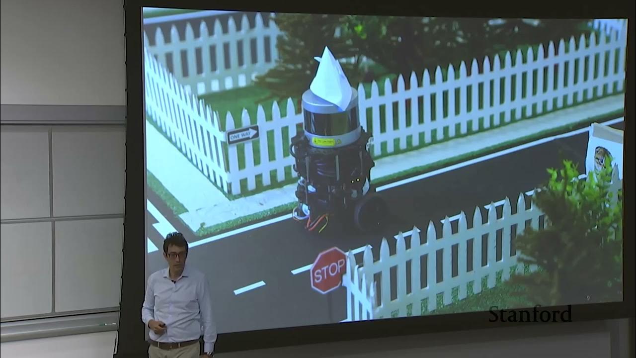
Continuing his overview of the hardware platform used in the course, Professor Marco Pavone explains that each robotic car is equipped with a top-mounted laser sensor, a camera, and a "beefy processor" capable of handling all computation directly onboard. Every one of the four autonomy modules—perception, localization, and the rest of the stack—runs directly on the robot as it works to accomplish a physical task. To illustrate what this looks like in practice, he recalls last year's culminating challenge: students had to program their robots to drive autonomously through a mock urban environment while reasoning about traffic signs. That single behavior required a full end-to-end pipeline: first detecting a sign, second placing it accurately within a metric map, third classifying its meaning—understanding that "this is a stop sign, it's not a speed limit sign"—and finally acting accordingly. The quarter concluded with a final competition among the student projects, and the specific project details for the current year will be disclosed later in the quarter.
To support students through this hands-on work, the class has five Course Assistants (CAs) whom Pavone will introduce shortly. "So they're going to be your best friends for this quarter," he jokes, advising the class, "So treat them well." In addition to frequent interaction with the CAs and other collaborators to be introduced later, the course labs leverage physical infrastructure from two Stanford facilities: Pavone's own Autonomous Systems Lab (ASL) and a lab at CARS, the Center for Automotive Research at Stanford.
The full syllabus is posted on the class website and divides the quarter into four modules of roughly equal length. The course begins with trajectory optimization and motion planning, then transitions into robot perception, where students study cameras, camera models, and how to extract both low-level geometric features (such as edges and corners) and high-level semantic information ("Is there a human or is there a cat in an image?") from image sensors. The third module tackles localization and mapping, starting with foundational background in probability theory and filtering theory before applying those tools via Kalman filtering and particle filtering. Finally, the fourth module covers decision-making, moving from finite state machines to methods for reasoning under uncertainty.
```mermaid flowchart LR accTitle: Four-Module Course Structure and Example Urban Driving Pipeline accDescr: Overview of the four core modules in AA274A alongside the four-step traffic sign reasoning task from the previous year's final project.
subgraph Syllabus["AA274A Core Syllabus Modules"] M1["1. Trajectory Optimization & Motion Planning"] --> M2["2. Robot Perception (Cameras, Edges, Object Detection)"] M2 --> M3["3. Localization & Mapping (Kalman & Particle Filtering)"] M3 --> M4["4. Decision Making (State Machines & Uncertainty)"] end
subgraph Project["Mock Urban Driving Task Pipeline"] P1["Detect Traffic Sign"] --> P2["Place Sign in Metric Map"] P2 --> P3["Classify Sign Type (e.g., Stop vs. Speed Limit)"] P3 --> P4["Execute Vehicle Action"] end ```
[14:43](https://www.youtube.com/watch?v=Lgt5ONBtFI0&t=883s) Q&A: Enrollment Limits, the Two-Quarter Sequence, and Course Logistics
Opening the floor to student questions, Pavone first addresses whether enrollment can be increased. He explains that the cap is strictly hardware-bound: the course has exactly 30 robots, and with students organized into teams of four, there is simply no physical capacity to accommodate more groups. Another student asks about the transition between the "A" and "B" courses, noting that this is the first year the class has been split into a two-quarter sequence. Pavone explains that the current autumn course (Principles of Robot Autonomy I) focuses almost entirely on classical autonomy techniques, whereas in the winter quarter he will co-teach the advanced sequel, Principles of Robot Autonomy II, alongside Professors Dorsa Sadigh and Jeannette Bohg. That winter course will follow the same pedagogical concept—students will incrementally build on top of the autonomous stack they created in the autumn—and will also be organized into four modules:
- **Module 1: Learning-Based Control and Perception** — Moving beyond the classical techniques of the first course to focus on machine learning approaches for perception and control. - **Module 2: Verification, Validation, and System Architecture** — Formal verification and validation of autonomous systems, alongside alternative ways of architecting the autonomy stack beyond the traditional "sense-think-act" paradigm. - **Module 3: Human-Robot Interaction** — Models and algorithms for interacting with humans, including human intent modeling. - **Module 4: Mobile Manipulation** — Extending mobile autonomy to physically manipulating objects in the environment.
Pavone also encourages students to enroll in the Friday Robotics Seminar that he co-organizes with Professor Jeannette Bohg, noting that it is a lightweight 1-unit course that offers a great way to stay current with active robotics research. Regarding units for AA274A itself, the course is offered for either 3 or 4 credits; the two options are identical except that 4-credit students must write a review of a research paper on robot autonomy toward the end of the quarter.
When a student asks how this autumn offering compares to the single-quarter AA274 course taught in the previous three years, Pavone admits that the old single-quarter version was "extremely packed." By splitting the sequence, he was able to offload machine learning topics to the winter course and add a Friday lecture session to unpack technical details that previously felt rushed. The extra breathing room also allowed him to introduce two brand-new topics to the autumn syllabus: a full week dedicated to multi-sensor perception (fusing information across multiple sensors) and a couple of lectures examining open-source autonomous driving software stacks, where collective community contributions are gaining real traction in industry. Rounding out the logistical questions, he clarifies cross-listing rules, exam scheduling, and the mysterious mechanics of the university registrar:
| Logistics Topic | Course Policy / Details | |:--- |:--- | | **Friday Lectures** | Required for all students enrolled in a 200-level listing (`AA274A`, `CS237A`, `EE260A`). Optional only for undergraduates enrolled under `AA174`. | | **Midterm Exams** | Held in class by default; alternate times can be arranged individually if a scheduling conflict arises. | | **Course Waitlists** | Although cross-listed sections (`AA`, `EE`, `CS`) display different waitlist numbers, all four waitlists pool into a single common waitlist managed by student priority ("the way the registrar office works is still a little bit mystery to me... Why is that in that way that is beyond my knowledge"). |
[20:38](https://www.youtube.com/watch?v=Lgt5ONBtFI0&t=1238s) Introduction to Mobile Robot Kinematics and Generalized Coordinates
Transitioning into the first technical lecture of the quarter—Mobile Robot Kinematics—Pavone explains why modeling is the prerequisite for everything in Module 1. To plan trajectories or design controllers, one first needs a mathematical model of the system. While some robots have a fixed base, such as a surgical robot, this course focuses primarily on mobile systems like self-driving cars and unmanned aircraft. Controlling the motion of a mobile robot requires modeling its dynamic evolution and, crucially, the physical constraints that govern how it can move. Pavone illustrates this with an everyday driving intuition: when driving a car, "you cannot move sideways," which is a fundamental constraint on instantaneous motion. Yet every driver knows that "by being clever in how you concatenate your backward and forward maneuver, you can go anywhere you want," provided there are no obstacles. The goal of kinematic modeling is to capture these constraints mathematically so a robot can reason about its maneuvers systematically.
Starting from first principles, a robot's configuration is defined by a set of **generalized coordinates**, denoted by the vector $\xi$, which represents the minimum set of coordinates required to uniquely specify the pose of the robot. To make this concrete, Pavone introduces an idealized single-wheeled robot rolling on a flat ground plane such that its sagittal plane—the plane containing the wheel itself—remains strictly orthogonal to the ground. While acknowledging with a smile that a lone wheel is not statically stable in the real world and would immediately tip over, he asks the class to "assume that we are in a world where a wheel can stay perfectly in balance."
Under this vertical-wheel assumption, the pose of the disk is completely described by three quantities relative to a fixed reference frame: - $x, y$: The planar coordinates of the center of the wheel. - $\theta$: The heading angle of the wheel with respect to the reference frame.
Because three independent parameters specify the wheel's pose, the **configuration space** for this idealized robot is three-dimensional, represented by $\xi = (x, y, \theta)$. From this perspective, the motion or **trajectory** of the system is simply the time evolution of its configuration variables.
[23:50](https://www.youtube.com/watch?v=Lgt5ONBtFI0&t=1430s) Holonomic Constraints and Degree-of-Freedom Reduction
The robot's trajectory is fundamentally a time-mapping function $s(t)$ into generalized configuration coordinates $s \in \mathbb{R}^n$, where $n$ represents the total number of configuration variables (such as $n = 3$ for the planar unicycle). However, a robot's motion is rarely unconstrained. The most familiar category of limitations consists of holonomic constraints, which depend exclusively on the configuration coordinates themselves rather than on their time derivatives. Expressed mathematically as a set of algebraic equations:
$$h_i(s) = 0, \quad i = 1, \dots, k$$
These equations directly reduce the robot's accessible configuration space, confining its permissible configurations to the level sets of the functions $h_i$.
In physical systems, holonomic constraints typically originate from rigid mechanical linkages and joints—such as prismatic or revolute joints in a robotic manipulator. These joints eliminate degrees of freedom and thereby reduce the number of independent generalized coordinates needed to fully characterize the robot's pose. To illustrate this concretely, consider a planar manipulator composed of two rigid links joined by a revolute joint that permits relative rotation. In isolation, each link is a planar rigid body possessing three degrees of freedom: link 1 is parameterized by position $(x_1, y_1)$ and heading $\theta_1$, while link 2 is parameterized by $(x_2, y_2)$ and heading $\theta_2$. Unconstrained, the combined system would require six configuration coordinates.
```mermaid flowchart TD accTitle: Holonomic Reduction of Two-Link Manipulator accDescr: Flowchart showing how six unconstrained planar coordinates are reduced to four generalized coordinates via two holonomic joint constraints. subgraph Initial["Unconstrained Links"] L1["Link 1: (x₁, y₁, θ₁)"] L2["Link 2: (x₂, y₂, θ₂)"] end subgraph Constraints["Revolute Joint Constraints"] C1["h₁(s): x₁ - x₂ = 0"] C2["h₂(s): y₁ - y₂ = 0"] end subgraph Reduced["Minimal Generalized Coordinates"] R["4 DOF: (x₁, y₁, θ₁, Δθ)"] end L1 --> C1 L2 --> C1 L1 --> C2 L2 --> C2 C1 --> R C2 --> R ```
The presence of the pin joint forces the connection points of the two bodies to coincide, imposing two distinct algebraic constraints:
$$x_1 = x_2 \implies h_1(s) = x_1 - x_2 = 0$$ $$y_1 = y_2 \implies h_2(s) = y_1 - y_2 = 0$$
Because these two constraints subtract two degrees of freedom from the original six-dimensional configuration space, exactly $6 - 2 = 4$ independent generalized coordinates are needed to describe the assembly. A common reduced parameterization chooses the base pose $(x_1, y_1, \theta_1)$ alongside the relative joint angle $\theta_2 - \theta_1$. For serial manipulators composed of revolute and prismatic joints, joint angles and link extensions routinely serve as this minimal coordinate set.
[27:47](https://www.youtube.com/watch?v=Lgt5ONBtFI0&t=1667s) Kinematic Constraints and the Pfaffian Form
A second, fundamentally critical class of constraints in mobile robotics consists of kinematic constraints. Unlike holonomic constraints, kinematic constraints explicitly involve both the generalized coordinates $s$ and their first time derivatives $\dot{s}$, where the dot notation signifies differentiation with respect to time ($\frac{d}{dt}$). Kinematic constraints govern the instantaneous admissible velocities of the mechanical system. A familiar real-world example is an automobile: at any instant, its wheels dictate that the vehicle cannot translate sideways.
In robotics, kinematic constraints are frequently expressed in Pfaffian form, meaning they are strictly linear in the generalized velocities $\dot{s}$, even if their dependence on the generalized coordinates $s$ is nonlinear:
$$a_i(s)^T \dot{s} = 0$$
Any holonomic constraint $h_i(s) = 0$ can trivially be converted into a Pfaffian kinematic constraint simply by differentiating it with respect to time using the chain rule:
$$\frac{d}{dt} h_i(s) = \nabla h_i(s)^T \dot{s} = 0$$
This raises an essential foundational question: does the converse always hold? Given an arbitrary Pfaffian kinematic constraint $a(s)^T \dot{s} = 0$, does there always exist an underlying algebraic function $h(s) = 0$ whose time derivative yields that exact constraint? When posed to the room, a student intuitively asks whether $h$ must equal zero and remarks, "Seems like you're gonna integrate that function... Unless the function is very weird, most nice functions are integrable, right?" The short answer is an emphatic no: in general, many kinematic constraints cannot be integrated back into configuration-level holonomic constraints.
- Kinematic constraints restrict instantaneous velocity vectors: $a(s)^T \dot{s} = 0$. - Holonomic constraints differentiate to Pfaffian kinematic constraints via $\frac{d}{dt}h(s) = \nabla h(s)^T \dot{s} = 0$. - The reverse question is an integrability problem that fails for general multivariable Pfaffian systems.
[32:05](https://www.youtube.com/watch?v=Lgt5ONBtFI0&t=1925s) Holonomic vs. Nonholonomic Constraints
Kinematic constraints that cannot be integrated into equivalent algebraic position constraints are formally termed nonholonomic constraints. The distinction between holonomic and nonholonomic constraints fundamentally alters how a robot can move:
| Constraint Type | Mathematical Form | Integrability | Geometric & Physical Consequence | |:--- |:--- |:--- |:--- | | **Holonomic** | $h(s) = 0$ (or $\dot{h}(s) = \nabla h^T \dot{s} = 0$) | Completely integrable | **Loss of accessibility:** Limits motion to an $(n-1)$-dimensional manifold/level set within $\mathbb{R}^n$. | | **Nonholonomic** | $a(s)^T \dot{s} = 0$ | Non-integrable | **Velocity restriction only:** Precludes certain instantaneous velocities, but preserves full reachability across the configuration space via sequencing maneuvers. |
When a constraint can be integrated into $h(s) = 0$, the system suffers a true loss of configuration accessibility. For instance, in a two-dimensional configuration space $(x_1, x_2)$, an algebraic constraint such as $x_1 + x_2 = 0$ traps the system on a one-dimensional line forever; it cannot explore the rest of the plane.
Nonholonomic constraints behave entirely differently. Because the constraint cannot be integrated, it restricts only the instantaneous velocities admissible at any particular state: > "With nonholonomic constraints you constrain the velocities but not the accessible portion of the configuration space. With holonomic constraints you constrain the accessible portion of the accessible space."
A car illustrates this contrast cleanly: at any given pose, the vehicle cannot slide sideways, meaning its lateral velocity component must be zero. Yet this lateral restriction does not prevent the driver from reaching any arbitrary coordinate in the plane. By concatenating forward, backward, and steering maneuvers—as one does when parallel parking—the vehicle can reach any desired position and heading $(x, y, \theta)$ in the configuration space.
[35:31](https://www.youtube.com/watch?v=Lgt5ONBtFI0&t=2131s) The Rolling Without Slipping Constraint in Wheeled Systems
Because the course focuses heavily on wheeled mobile robots, these constraint mechanics are applied directly to a wheel rolling on a plane, returning to the idealized unicycle model. The system is modeled as a vertical circular disk—comparable to a coin rolling on its edge—constrained to remain upright on its sagittal axis orthogonal to the plane.
The configuration of this single-wheel system is fully described by:
$$s = \begin{bmatrix} x \\ y \\ \theta \end{bmatrix}$$
where $(x, y)$ represents the Cartesian contact point of the wheel on the ground, and $\theta$ denotes the heading angle (orientation) of the wheel relative to the global reference frame.
The central physical assumption governing standard wheeled vehicles is rolling without slipping (pure rolling). This condition dictates that the instantaneous velocity of the contact point cannot have any component orthogonal to the wheel's sagittal plane. In geometric terms, the admissible velocity vector must align with the wheel's heading, forming a 90-degree angle with the lateral axis. The wheel is physically forbidden from moving sideways across the ground surface, establishing the foundational nonholonomic velocity constraint of wheeled mobile robotics.
[37:12](https://www.youtube.com/watch?v=Lgt5ONBtFI0&t=2232s) Deriving the Pure Rolling Pfaffian Constraint
To formalize the pure rolling condition, the velocity of the wheel's contact point cannot have any component orthogonal to the wheel's sagittal plane. Representing the rolling disc or coin on a horizontal 2D plane, its orientation is defined by the heading angle $\theta$ measured relative to a reference coordinate axis. A unit vector in the direction of the contact point's forward velocity is defined as:
$$e_v = \begin{bmatrix} \cos\theta \\ \sin\theta \end{bmatrix}$$
Because $e_v$ is a unit vector of length 1, its Cartesian coordinates are directly given by $\cos\theta$ and $\sin\theta$.
To express the requirement that the wheel cannot slide sideways, an orthogonal unit vector $e_v^\perp$ is constructed perpendicular to $e_v$. Using the geometric angle $\frac{\pi}{2} - \theta$, its coordinates evaluate to:
$$e_v^\perp = \begin{bmatrix} \cos\left(\frac{\pi}{2} - \theta\right) \\ -\sin\left(\frac{\pi}{2} - \theta\right) \end{bmatrix} = \begin{bmatrix} \sin\theta \\ -\cos\theta \end{bmatrix}$$
Taking the inner product $e_v \cdot e_v^\perp = \cos\theta\sin\theta - \sin\theta\cos\theta = 0$ confirms that the two vectors are strictly orthogonal.
The no-side-slip condition stipulates that the planar velocity vector $v = [\dot{x}, \dot{y}]^T$ must have zero projection along $e_v^\perp$:
$$\begin{bmatrix} \dot{x} \\ \dot{y} \end{bmatrix} \cdot e_v^\perp = 0 \implies \dot{x}\sin\theta - \dot{y}\cos\theta = 0$$
This relation is the classic Pfaffian constraint governing a rolling disc on a plane. It is classified as Pfaffian because its dependence on the generalized velocity coordinates $(\dot{x}, \dot{y})$ is strictly linear, whereas its dependence on the generalized configuration coordinate $\theta$ is nonlinear through sine and cosine functions.
When a student asks how this expression relates to the full configuration vector $\xi = [x, y, \theta]^T$, the instructor clarifies that in canonical Pfaffian form, the constraint is written against the complete vector of generalized velocities $\dot{\xi} = [\dot{x}, \dot{y}, \dot{\theta}]^T$:
$$\begin{bmatrix} \sin\theta & -\cos\theta & 0 \end{bmatrix} \begin{bmatrix} \dot{x} \\ \dot{y} \\ \dot{\theta} \end{bmatrix} = 0$$
The zero in the final component cancels out $\dot{\theta}$, leaving the planar no-slip equation intact while maintaining standard matrix form across the entire configuration space.
[42:11](https://www.youtube.com/watch?v=Lgt5ONBtFI0&t=2531s) Accessibility vs. Admissible Motion and Nonholonomy
Although the pure rolling constraint restricts the instantaneous admissible velocities—prohibiting the disc from sliding sideways at any given instant—it does not cause any loss of reachable configuration space (accessibility). The disc can still reach any arbitrary planar position and orientation $(x, y, \theta)$ through a straightforward three-point maneuver:
```mermaid flowchart LR accTitle: Three-Point Maneuver Sequence accDescr: Sequence showing how a nonholonomic vehicle navigates from an initial state to a target state using three discrete steps. A["Initial Pose (x_0, y_0, θ_0)"] -->|"Rotate in place"| B["Heading Aligned with Target"] B -->|"Drive Straight"| C["Arrive at Position (x_f, y_f)"] C -->|"Rotate in place"| D["Final Pose (x_f, y_f, θ_f)"] ```
1. **Rotate in place** from the initial heading $\theta_0$ until the wheel points directly toward the target position $(x_f, y_f)$. 2. **Drive in a straight line** along that line of sight until reaching $(x_f, y_f)$. 3. **Rotate in place once more** to match the desired final heading $\theta_f$.
This geometric construction provides an intuitive physical proof that non-integrable velocity constraints limit *admissible motions* rather than *reachable configurations*. Wheeled mobile robots are fundamentally nonholonomic systems for this exact reason.
In response to a student question pointing out that the ideal disc model leaves $\dot{\theta}$ completely unbounded, the instructor notes that while real physical systems cannot rotate infinitely fast, this unconstrained model serves to isolate the core mathematics of nonholonomy. More realistic kinematic models with steering limits and bounded velocities are developed later in the course. The instructor emphasizes a core takeaway: robotic manipulators are primarily characterized by holonomic constraints (closed kinematic loops reducing degrees of freedom), whereas wheeled mobile robots are dominated by nonholonomic constraints that restrict velocity directions without reducing positional reach.
[44:07](https://www.youtube.com/watch?v=Lgt5ONBtFI0&t=2647s) Taxonomy of Wheels: Standard, Steerable, and Caster
To bridge theoretical disc rolling to real ground robots, the lecture examines common wheel mechanical designs:
- **Fixed Standard Wheels**: A conventional wheel that freely rotates about a horizontal axle passing through its geometric center and orthogonal to the sagittal plane, but has a fixed orientation relative to the chassis. It cannot rotate around a vertical steering axis. A typical example is the rear pair of wheels on a standard grocery shopping cart, which provide directional stability. - **Steerable Standard Wheels**: Mechanically identical to a fixed standard wheel, with the addition of an active or passive mechanism permitting rotation around a vertical axis passing directly through the wheel's center and its ground contact point. - **Caster Wheels**: Commonly seen on the front of grocery carts or office chairs. Unlike standard steerable wheels, the vertical axis of rotation is offset by a lever arm relative to the wheel axle. Because of this mechanical offset, lateral forces exert a torque that automatically swivels the wheel into alignment with the robot's direction of travel. Caster wheels combine directional compliance for maneuverability with the support of the vehicle base. - **Active vs. Passive Actuation**: Active wheels are driven or steered by dedicated actuators/motors, whereas passive wheels (such as unpowered shopping cart casters) freely track the external lateral motions dictated by the chassis. - **Advanced Wheel Variants**: Mention is made of Swedish (Mecanum) wheels and omnidirectional wheels with transverse rollers, though standard and caster wheels form the primary focus of the course.
[48:17](https://www.youtube.com/watch?v=Lgt5ONBtFI0&t=2897s) Matrix Formulation of Pfaffian Constraints and the Null Space
For a multi-wheeled mobile robot equipped with $k$ wheels, each wheel introduces its own no-side-slip condition, generating a set of $k$ kinematic constraints. These constraints are stacked into a compact matrix equation:
$$A^T(\xi)\dot{\xi} = 0$$
where $\xi \in \mathbb{R}^n$ is the generalized configuration vector, $\dot{\xi} \in \mathbb{R}^n$ represents the generalized velocities, and $A^T(\xi) \in \mathbb{R}^{k \times n}$ is the configuration-dependent constraint matrix whose rows represent the individual wheel constraints.
Addressing a student inquiry regarding whether every kinematic constraint can be cast in Pfaffian form, the instructor notes that while general kinematic constraints in mechanics need not be Pfaffian, the non-slip rolling constraints of standard wheeled platforms are almost universally linear in velocity, and thus Pfaffian form is standard for ground robotics.
Geometrically and algebraically, the condition $A^T(\xi)\dot{\xi} = 0$ dictates that at any robot configuration $\xi$: - The set of all kinematically admissible generalized velocities $\dot{\xi}$ must lie entirely within the **null space** (or kernel) of the constraint matrix $A^T(\xi)$: $$\dot{\xi} \in \operatorname{Null}\left(A^T(\xi)\right)$$ - If the configuration space has dimension $n$ and there are $k$ independent constraints, the null space has dimension $n - k$, which defines the instantaneous velocity degrees of freedom available to the system.
[50:19](https://www.youtube.com/watch?v=Lgt5ONBtFI0&t=3019s) Deriving Admissible Velocities from Pfaffian Constraints
To generalize motion constraints across any robotic platform, multiple Pfaffian constraints can be stacked into a single matrix equation. If there are multiple constraints—for instance, $a_1^T \dot{q} = 0$ (such as the unicycle's lateral constraint $[\sin\theta, -\cos\theta, 0]\dot{q} = 0$) and $a_2^T \dot{q} = 0$—they can be compacted by defining a matrix $A^T$ containing each constraint vector as a row, resulting in $A(q)^T \dot{q} = 0$. Consequently, the admissible velocities $\dot{q}$ for the system are precisely those that lie within the null space (or kernel) of the constraint matrix $A^T$.
```mermaid flowchart LR accTitle: Pfaffian Constraints to Kinematic Model Pipeline accDescr: Diagram illustrating how kinematic constraints are stacked into matrix form, analyzed via null space, and transformed into kinematic equations of motion.
subgraph MatrixForm["Constraint Formulation"] C["Pfaffian Constraints<br/>a_i(q)^T q_dot = 0"] --> M["Stack Rows<br/>A(q)^T q_dot = 0"] end
subgraph LinearAlgebra["Kernel Analysis"] M --> K["Compute Null Space<br/>Kernel of A(q)^T"] K --> B["Select Basis Vectors<br/>{g_1(q),..., g_m(q)}"] end
subgraph Kinematics["Equations of Motion"] B --> E["Linear Combination<br/>q_dot = sum(g_j * u_j)"] end ```
By applying basic linear algebra, any vector in the kernel can be written as a linear combination of its basis vectors. If the robot's configuration space has dimension $n = 3$ and there is only one constraint (a single row in $A^T$), the dimension of the null space is $n - 1 = 2$. Therefore, the kernel can be spanned by two linearly independent basis vectors, and the velocity vector $\dot{q}$ is expressed as a linear combination of those basis vectors scaled by control inputs $u_j$: $$\dot{q} = \sum_{j=1}^{m} g_j(q) u_j$$ This establishes a systematic recipe for deriving kinematic models across robotics: collect all no-slip or mechanical constraints, stack them into $A^T$, determine the kernel of the matrix, pick an appropriate basis, and express the state velocity as the superposition of those basis vectors modulated by control inputs.
[53:35](https://www.youtube.com/watch?v=Lgt5ONBtFI0&t=3215s) Derivation of the Celebrated Unicycle Model
Returning to the unicycle example illustrates how this linear algebraic procedure produces the standard kinematic equations. The unicycle operates in a three-dimensional configuration space $q = [x, y, \theta]^T$, and pure rolling without lateral slipping yields a single constraint row: $$A(q)^T = \begin{bmatrix} \sin\theta & -\cos\theta & 0 \end{bmatrix}$$ Because $A^T$ has rank 1 in a 3D configuration space, its kernel is two-dimensional and requires two basis vectors. While there is freedom in choosing the basis, a particularly natural and physically meaningful choice is: $$g_1(q) = \begin{bmatrix} \cos\theta \\ \sin\theta \\ 0 \end{bmatrix}, \quad g_2(q) = \begin{bmatrix} 0 \\ 0 \\ 1 \end{bmatrix}$$ Multiplying $A(q)^T$ by $g_1(q)$ yields $\sin\theta\cos\theta - \cos\theta\sin\theta + 0 = 0$, and multiplying by $g_2(q)$ yields 0, confirming both vectors lie in the kernel. Since they are linearly independent, they form a valid basis, yielding the "celebrated unicycle model": $$\begin{bmatrix} \dot{x} \\ \dot{y} \\ \dot{\theta} \end{bmatrix} = \begin{bmatrix} \cos\theta \\ \sin\theta \\ 0 \end{bmatrix} v + \begin{bmatrix} 0 \\ 0 \\ 1 \end{bmatrix} \omega$$
- The scalar scaling factors act directly as control inputs: $v$ represents the linear driving speed (the magnitude of the velocity at the ground contact point), while $\omega = \dot{\theta}$ represents the angular speed. - In practical implementations, the unicycle model is augmented with actuator constraints, imposing bounds on maximum forward speed ($|v| \le v_{\max}$) and maximum turning rate ($|\omega| \le \omega_{\max}$). - Although AA274A focuses predominantly on this model, this systematic derivation applies universally to cars, aircraft, and tractor-trailers, allowing students to extract standard kinematic models from robotics literature without re-deriving them from scratch.
[57:10](https://www.youtube.com/watch?v=Lgt5ONBtFI0&t=3430s) Differential Drive Robots and Kinematic Equivalence
In the physical world, an actual unicycle or rolling disk is statically unstable and will simply fall over on its side. To achieve static stability while retaining simple kinematics, robotics relies heavily on the differential drive platform—the very architecture used by the course's physical lab robots. A differential drive robot features two independent, fixed active wheels mounted on a common rear axle, accompanied by a passive front caster wheel that pivots freely to match lateral motion without imposing any kinematic side-slip constraints.
```mermaid flowchart TD accTitle: Differential Drive Configuration and Constraints accDescr: Structural layout of a differential drive robot showing the two independent rear drive wheels on a shared axle and the front passive caster wheel.
subgraph Front["Front Support"] Caster["Passive Caster Wheel<br/>(Aligns freely, 0 constraints)"] end
subgraph Rear["Rear Drive Axle"] WL["Left Drive Wheel<br/>(Rotational speed omega_L)"] WR["Right Drive Wheel<br/>(Rotational speed omega_R)"] Axle["Common Axis Connecting Wheel Centers"] WL --- Axle --- WR end
Front --- Rear ```
Because the two rear wheels share a rigid axle, asserting that the left wheel cannot slip sideways inherently prevents the right wheel from slipping sideways as well. Consequently, the two lateral no-slip conditions are mathematically redundant and collapse into a single constraint. Since the passive caster wheel adds no nonholonomic constraints, the differential drive possesses the exact same kinematic constraints and null-space structure as the idealized unicycle.
- When the rear wheels are driven differentially—for example, the left wheel moving backward while the right wheel moves forward—the chassis rotates in place. - Unlike the unicycle model, which assumes direct control of forward speed $v$ and turn rate $\omega$, a physical differential drive robot is actuated via the rotational speeds of its left and right wheels ($\omega_L$ and $\omega_R$). - A student points out that while the kinematics are identical, actuator velocity limits differ: bounding individual wheel speeds ($\omega_L, \omega_R$) produces a coupled limit on the permissible combinations of $(v, \omega)$, distinguishing the achievable control envelope from an independently bounded unicycle. - Relating wheel angular velocities to chassis velocities $(v, \omega)$ requires examining the circular geometry of the robot's motion about its instantaneous center of rotation during turning maneuvers.
[01:02:30](https://www.youtube.com/watch?v=Lgt5ONBtFI0&t=3750s) Kinematic Equivalence: Differential Drive to Unicycle Model
The discussion focuses on the motion of a differential drive robot rotating around a point on the axis connecting its two rear wheel centers: the instantaneous center of rotation (ICR), also called the instantaneous curvature center. If the vehicle maintains a constant velocity vector, it traces a circular path centered at this ICR. Defining $\omega$ as the instantaneous angular velocity around the ICR, $V$ as the linear forward speed at the midpoint of the rear axle, and $R$ as the radius of curvature (the distance from the midpoint to the ICR), the basic relation holds: $V = \omega R$.
```mermaid flowchart LR accTitle: Unicycle to Differential Drive Mapping accDescr: Diagram showing planning in unicycle coordinates and mapping to individual wheel speeds. subgraph Planning ["Trajectory Planning"] U["Unicycle Model<br/>(V, ω)"] end subgraph Mapping ["Kinematic Mapping"] M1["V = (V_R + V_L) / 2"] M2["ω = (V_R - V_L) / L"] end subgraph Actuation ["Wheel Actuation"] W["Wheel Angular Speeds<br/>(ω_L, ω_R via radius r)"] end U --> Mapping Mapping --> Actuation ```
Let $L$ represent the chassis track width (the distance between the two wheels). The individual wheel linear velocities are given by $V_L = \omega (R - L/2)$ for the left wheel and $V_R = \omega (R + L/2)$ for the right wheel, because the entire chassis behaves as a rigid body sharing the same angular rate $\omega$. Taking the difference yields:
$$V_R - V_L = \omega L \implies \omega = \frac{V_R - V_L}{L}$$
A student points out a missing factor during the board derivation (where a division by 2 was momentarily written instead of $L$), which Pavone quickly corrects with an "Oops" and a chuckle, noting that dimensionally it must divide by $L$. Intuition confirms this equation: when $V_R = V_L$, the angular velocity $\omega$ is zero, meaning the robot drives straight ahead; if $V_L = 0$ while $V_R > 0$, the robot rotates directly around its stationary left wheel.
Summing the two velocities yields $V_L + V_R = 2\omega R = 2V$, proving that the midpoint forward speed is simply the average of the two wheel speeds:
$$V = \frac{V_R + V_L}{2}$$
Finally, relating the linear speeds of each wheel to their individual rotational rates through the wheel radius $r$ ($V_L = \omega_L r$ and $V_R = \omega_R r$) completes a clean, one-to-one mapping between the unicycle model inputs $(V, \omega)$ and the physical wheel controls $(\omega_L, \omega_R)$. Consequently, trajectory planners can operate entirely in terms of the simpler unicycle model and then map those trajectories directly down to the physical wheel actuators.
- $V = \omega R$ (midpoint speed as a function of angular rate and turning radius) - $V = \frac{V_R + V_L}{2}$ (midpoint speed as the average of left and right wheel velocities) - $\omega = \frac{V_R - V_L}{L}$ (angular velocity driven by speed difference across track width $L$) - $V_L = \omega_L r$ and $V_R = \omega_R r$ (conversion between linear wheel speed and wheel spin rate via wheel radius $r$)
---
[01:09:11](https://www.youtube.com/watch?v=Lgt5ONBtFI0&t=4151s) The Simple Car, Reeds-Shepp, and Dubins Models
In response to a student question about potential singularities (such as a passive caster wheel turning perpendicular to the direction of travel), Pavone transitions to models with explicit steering mechanisms, introducing the simple car model (often analyzed in equivalent form as a bicycle model). Unlike the differential drive platform, the simple car features fixed rear wheels alongside steerable front wheels.
This system is described by a four-dimensional configuration space $(x, y, \theta, \phi)$, representing the $(x, y)$ position of the rear axle midpoint, the vehicle heading $\theta$, and the front wheel steering angle $\phi$ relative to the longitudinal axis. The kinematics must satisfy two non-redundant no-side-slip constraints: one for the rear wheels and one for the front wheels. Because there are four configuration variables and two independent nonholonomic constraints, the null space of allowable motions is two-dimensional. The two primary control inputs are the driving velocity $V$ and the steering angle $\phi$ (or steering rate).
Different operational bounds imposed on these inputs give rise to classical motion planning models: - **Simple Car Model**: Linear velocity $V$ and steering angle $\phi$ are bounded. Singularity is avoided by enforcing $|\phi| < \frac{\pi}{2}$. - **Reeds-Shepp Car**: The steering angle remains bounded, while the velocity is constrained to discrete forward and reverse driving speeds ($V \in \{-V_{\max}, +V_{\max}\}$). - **Dubins Car**: The vehicle can only drive forward at a fixed maximum speed ($V = V_{\max}$) with bounded steering, a staple model widely studied in motion planning and optimal path synthesis.
For deeper derivations and discussions of kinematic constraints and singularities, Pavone points students to classical literature, including Steven M. LaValle's *Planning Algorithms*.
---
[01:12:31](https://www.youtube.com/watch?v=Lgt5ONBtFI0&t=4351s) Bridging Kinematics to Dynamics in Trajectory Planning
Pavone addresses the relationship between pure kinematic formulations and real-world vehicle dynamics. He emphasizes that a kinematic state-space model must always be understood merely as a simplified subsystem of a full dynamic model. Robotics engineers deliberately rely on kinematic models during trajectory optimization because their lower dimensionality keeps optimization problems computationally tractable. A lower-level tracking controller or "black-box module" then handles the translation of kinematic commands $(V, \omega)$ into true dynamical control actions, such as linear and angular accelerations or motor torques.
Alternatively, model fidelity can be enhanced without full dynamic modeling by adding integrators to the kinematic state: - For the unicycle model, velocity $V$ can be elevated from an input to a state variable by adding the integrator $\dot{V} = a$, where acceleration $a$ becomes the new control input (an approach utilized in the course's first problem set). - For the simple car, the steering angle $\phi$ can become a state variable with its derivative governed by a steering rate input: $\dot{\phi} = u_\phi$.
Engineering autonomous vehicles involves navigating a fundamental tension: > "On the one hand, you want to have a model that is representative enough of the dynamics so that when you plan a trajectory, the trajectory is realizable. On the other hand, you don't want to have a model that is too complicated because trajectory optimization, as we will see next week, is a computationally intensive process."
Balancing fidelity against computational feasibility remains "a bit of an art." In AA274A, the focus is placed on striking this balance specifically for wheeled systems and differential drive robots. Wrapping up the lecture, Pavone previews the upcoming schedule: the following lecture will introduce ROS (Robot Operating System), followed by an inspirational robotics lecture on Friday.
[01:14:56](https://www.youtube.com/watch?v=Lgt5ONBtFI0&t=4496s) Guest Speaker Preview and Upcoming Topics
Prof. Pavone concludes the lecture by looking ahead to upcoming sessions on the syllabus. He previews an upcoming guest appearance by a personal friend who serves as the CEO of an autonomous trucking company, who will visit the class to discuss the practical realities and engineering challenges of fielding autonomous systems in the real world.
Looking further into the course roadmap, Pavone notes that next week's lectures will turn toward the core algorithmic foundations of motion, specifically focusing on trajectory optimization, trajectory tracking, and feedback control. He leaves the class with a reminder about the guest appearance scheduled for Thursday with Bret Jones.
- **Upcoming Guest Lecture**: Bret Jones (CEO of an autonomous truck company) presenting on the practical hurdles of deploying autonomous platforms in real-world environments. - **Next Week's Curriculum**: Trajectory optimization, trajectory tracking, and robot control systems.
## Notable quotes > [08:02](https://www.youtube.com/watch?v=Lgt5ONBtFI0&t=482s) Frustration is in the DNA of every roboticist — Prof. Marco Pavone
> [12:08](https://www.youtube.com/watch?v=Lgt5ONBtFI0&t=728s) So they're going to be your best friends for this quarter — Prof. Marco Pavone
> [14:43](https://www.youtube.com/watch?v=Lgt5ONBtFI0&t=883s) the way the registrar office works is still a little bit mystery to me... Why is that in that way that is beyond my knowledge — Prof. Marco Pavone
> [20:38](https://www.youtube.com/watch?v=Lgt5ONBtFI0&t=1238s) you cannot move sideways — Prof. Marco Pavone
> [20:38](https://www.youtube.com/watch?v=Lgt5ONBtFI0&t=1238s) by being clever in how you concatenate your backward and forward maneuver, you can go anywhere you want — Prof. Marco Pavone
> [20:38](https://www.youtube.com/watch?v=Lgt5ONBtFI0&t=1238s) assume that we are in a world where a wheel can stay perfectly in balance. — Prof. Marco Pavone
> [27:47](https://www.youtube.com/watch?v=Lgt5ONBtFI0&t=1667s) Seems like you're gonna integrate that function... Unless the function is very weird, most nice functions are integrable, right? — Student
> [32:05](https://www.youtube.com/watch?v=Lgt5ONBtFI0&t=1925s) With nonholonomic constraints you constrain the velocities but not the accessible portion of the configuration space. With holonomic constraints you constrain the accessible portion of the accessible space. — Prof. Marco Pavone
> [01:12:31](https://www.youtube.com/watch?v=Lgt5ONBtFI0&t=4351s) On the one hand, you want to have a model that is representative enough of the dynamics so that when you plan a trajectory, the trajectory is realizable. On the other hand, you don't want to have a model that is too complicated because trajectory optimization, as we will see next week, is a computationally intensive process. — Prof. Marco Pavone
## Mentioned Marco Pavone, Dorsa Sadigh, Jeannette Bohg, Steven M. LaValle, Bret Jones, Stanford University, Autonomous Systems Lab (ASL), Center for Automotive Research at Stanford (CARS), NASA Jet Propulsion Laboratory (JPL), NVIDIA, Amazon, Airbus, Fiat, Robot Operating System (ROS), Python, Principles of Robot Autonomy, Planning Algorithms, Piazza
## Video description For more information about Stanford’s graduate programs, visit: https://online.stanford.edu/graduate-education
Lecture 1 — Course Overview, Mobile Robot Kinematics
Note: This lecture was recorded as part of the 2019 edition of the course. Course content, structure, assignments, and other materials may have changed since this recording. The course links below point to the most recent edition and may therefore differ from what is presented in the video.
Read the companion textbook, Principles of Robot Autonomy, free online: https://porabook.com
Follow along with the latest course schedule and syllabus: https://stanfordasl.github.io/PoRA-I
Speaker: Prof. Marco Pavone
Dr. Marco Pavone is an Associate Professor of Aeronautics and Astronautics at Stanford University and a Senior Director of Autonomous Vehicle Research at NVIDIA. Prior to joining Stanford, he was a Research Technologist in the Robotics Section at NASA’s Jet Propulsion Laboratory. Dr. Pavone received his Ph.D. in Aeronautics and Astronautics from the Massachusetts Institute of Technology in 2010. His research focuses on the analysis, design, and control of autonomous systems, with particular emphasis on self-driving cars, autonomous aerospace vehicles, and future mobility systems. He has been recognized with numerous awards, including the Presidential Early Career Award for Scientists and Engineers from President Barack Obama, the Office of Naval Research Young Investigator Award, the NSF CAREER Award, the NASA Early Career Faculty Award, the IEEE Kiyo Tomiyasu Award, the CSS Award for Technical Excellence in Aerospace Control, and the Early-Career Spotlight Award from the Robotics Science and Systems Foundation.
Full playlist: https://www.youtube.com/playlist?list=PLR9iNyexfIkk
#StanfordOnline #RobotAutonomy #Robotics #PhysicalAI
[Source](https://www.youtube.com/watch?v=Lgt5ONBtFI0)