Pavone Cuts Robot Trajectory Compute Using Differential Flatness Maps
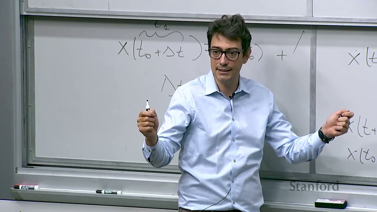
Stanford AA274A Principles of Robotic Autonomy | Autumn 2019 | Trajectory Optimization — Stanford Online

Stanford Online

Differential flatness allows autonomous vehicles to bypass differential equation integration by algebraically reconstructing full system states and control inputs from smooth curves planned in a lower-dimensional output space.

AI-assisted summary of Stanford AA274A Principles of Robotic Autonomy | Autumn 2019 | Trajectory Optimization — original source. Check the original for full context.

Source published:

Key ideas

  • Differential flatness eliminates the need to integrate non-linear differential equations during planning by establishing an algebraic mapping between system states, control inputs, and a reduced coordinate space of flat outputs. (54:07)
  • Autonomous robotics circumvents the prohibitive computational cost of full-state closed-loop optimal control by utilizing a two-step architecture: generating an open-loop nominal reference trajectory and stabilizing it locally with a feedback tracking controller. (30:08)
  • Numerical open-loop trajectory optimization is split into direct methods, which discretize continuous dynamics into finite-dimensional nonlinear programs, and indirect methods, which derive variational boundary-value differential equations before discretization. (33:33)
  • Minimizing higher-order derivatives like jerk and snap provides a computationally efficient proxy for reducing actuator effort, serving as the design standard for roughly 95% of quadrotor trajectory planning algorithms. (66:25)

Detailed notes

## Background Published on YouTube by Stanford Online on October 9, 2026, this video documents Lecture 3 of the Autumn 2019 Stanford course AA274A (Principles of Robotic Autonomy), presented by Prof. Marco Pavone. According to the description, the session focuses on trajectory optimization, open-loop motion control, and differential flatness, providing theoretical foundations supported by the free companion textbook Principles of Robot Autonomy.

## TL;DR Prof. Marco Pavone formulates the trajectory optimization problem for autonomous robots, distinguishing between computationally intensive closed-loop policies and practical two-step architectures that pair open-loop nominal references with local feedback tracking. After contrasting direct discretization approaches with indirect variational methods, the lecture pivots to differential flatness as an efficient method for generating dynamically feasible paths without numerical integration. Using the kinematic simple car model, Pavone demonstrates how planning smooth polynomial curves in flat output coordinates allows full vehicle states and control inputs to be recovered algebraically. He concludes by detailing objective criteria such as minimum-snap optimization and explaining how actuator limits are handled via time scaling.

## Atmosphere & style The lecture carries an engaging, approachable academic atmosphere driven by Prof. Pavone's conversational teaching style and clear enthusiasm for robotics engineering. Theoretical derivations of differential equations and flatness mappings are regularly interspersed with spontaneous classroom demonstrations, student interactions, and lighthearted humor regarding childhood tricycles and dead-reckoning navigation. Watching the session feels like attending a rigorous yet demystifying graduate engineering workshop where complex mathematical abstractions are systematically translated into pragmatic, implementable autonomy algorithms.

## Bulletin - [54:07](https://www.youtube.com/watch?v=Kv5G2OlrIbU&t=3247s) Differential flatness eliminates the need to integrate non-linear differential equations during planning by establishing an algebraic mapping between system states, control inputs, and a reduced coordinate space of flat outputs. - [30:08](https://www.youtube.com/watch?v=Kv5G2OlrIbU&t=1808s) Autonomous robotics circumvents the prohibitive computational cost of full-state closed-loop optimal control by utilizing a two-step architecture: generating an open-loop nominal reference trajectory and stabilizing it locally with a feedback tracking controller. - [33:33](https://www.youtube.com/watch?v=Kv5G2OlrIbU&t=2013s) Numerical open-loop trajectory optimization is split into direct methods, which discretize continuous dynamics into finite-dimensional nonlinear programs, and indirect methods, which derive variational boundary-value differential equations before discretization. - [01:06:25](https://www.youtube.com/watch?v=Kv5G2OlrIbU&t=3985s) Minimizing higher-order derivatives like jerk and snap provides a computationally efficient proxy for reducing actuator effort, serving as the design standard for roughly 95% of quadrotor trajectory planning algorithms.

## Key takeaways - [01:01](https://www.youtube.com/watch?v=Kv5G2OlrIbU&t=61s) Trajectory optimization computes a continuous time history of states and control inputs that steers a robot between boundary conditions while honoring physical and kinematic constraints. - [06:50](https://www.youtube.com/watch?v=Kv5G2OlrIbU&t=410s) Forward Euler discretization models continuous differential equations into discrete updates, presenting a core robotic trade-off between numerical fidelity and computational runtime. - [16:37](https://www.youtube.com/watch?v=Kv5G2OlrIbU&t=997s) Optimal control cost functions rely on an additive structure combining terminal penalties and integrated running costs to ensure mathematical tractability under dynamic programming principles. - [21:44](https://www.youtube.com/watch?v=Kv5G2OlrIbU&t=1304s) Trajectory optimization formally addresses dynamic feasibility in unconstrained state space, whereas motion planning addresses the non-convex complexity of explicit state constraints such as obstacle avoidance. - [24:56](https://www.youtube.com/watch?v=Kv5G2OlrIbU&t=1496s) Open-loop control profiles match closed-loop policies in deterministic theory, but real-world unmodeled dynamics and disturbances inevitably cause uncorrected open-loop systems to drift. - [30:08](https://www.youtube.com/watch?v=Kv5G2OlrIbU&t=1808s) Practical autonomy applies a two-step compromise that executes an open-loop nominal path while restricting feedback control effort to a local operating tube around the reference. - [34:40](https://www.youtube.com/watch?v=Kv5G2OlrIbU&t=2080s) Direct methods convert continuous optimal control into solvable nonlinear programs via Riemann summation and Euler integration constraints. - [37:46](https://www.youtube.com/watch?v=Kv5G2OlrIbU&t=2266s) Indirect methods apply the calculus of variations to derive first-order necessary conditions of optimality, formulating differential boundary value problems that require numerical solution. - [43:20](https://www.youtube.com/watch?v=Kv5G2OlrIbU&t=2600s) Fast replenishment rates of 1 to 10 Hz in dynamic environments make discovering kinematically feasible trajectories far more practical than solving exhaustive optimal control problems. - [50:00](https://www.youtube.com/watch?v=Kv5G2OlrIbU&t=3000s) In a kinematic simple car, rear axle coordinates completely determine vehicle heading and input commands algebraically, avoiding differential equation integration. - [54:07](https://www.youtube.com/watch?v=Kv5G2OlrIbU&t=3247s) A system is differentially flat when there exist flat outputs equal in number to system inputs that algebraically reconstruct all states and inputs using finite time derivatives. - [59:07](https://www.youtube.com/watch?v=Kv5G2OlrIbU&t=3547s) Trajectory generation for flat systems follows a three-step pipeline: mapping boundary conditions, interpolating a smooth curve in flat output space, and algebraically evaluating states and controls. - [01:02:15](https://www.youtube.com/watch?v=Kv5G2OlrIbU&t=3735s) Representing flat outputs through polynomial basis functions reduces continuous path planning to linear constraint satisfaction or low-dimensional coefficient optimization. - [01:06:25](https://www.youtube.com/watch?v=Kv5G2OlrIbU&t=3985s) Penalizing higher-order time derivatives—such as acceleration, jerk, and snap—smooths trajectory geometry and minimizes aggressive actuator saturation. - [01:09:32](https://www.youtube.com/watch?v=Kv5G2OlrIbU&t=4172s) Time scaling decouples geometric path synthesis from actuator limits by reparameterizing time along a flat trajectory until control bounds are satisfied. - [01:10:45](https://www.youtube.com/watch?v=Kv5G2OlrIbU&t=4245s) Control theory lacks a constructive computational procedure to test whether an arbitrary nonlinear dynamical system is differentially flat.

## Detailed walkthrough ### [00:06](https://www.youtube.com/watch?v=Kv5G2OlrIbU&t=6s) Course Logistics and the Role of ROS in Discussion Sections

Professor Marco Pavone opens the lecture by recapping the foundational ground covered during the first week. The opening lecture established the kinematic and dynamic models of robot motion, followed by an introductory orientation to the Robot Operating System (ROS). Moving forward, students will gain significantly deeper exposure to ROS during their weekly discussion sections. In the current week, students will set up the requisite software environments and development toolchains on their machines, while the following week's sections will guide them through building and executing their first live ROS nodes.

Pavone highlights the instructional philosophy behind this structure: the bulk of hands-on software engineering and coding activities are intentionally delegated to discussion sections. The teaching team found this interactive approach to be "a particularly effective way to teach you how to do things by having you doing things while having a CA watching you." This direct supervision from Course Assistants ensures that practical tooling hurdles and debugging issues are addressed immediately in an active lab setting rather than becoming roadblocks during assignments.

[01:01](https://www.youtube.com/watch?v=Kv5G2OlrIbU&t=61s) Defining the Trajectory Optimization Problem

Transitioning from system modeling to planning, the lecture pivots to leveraging kinematic and dynamic equations to generate robotic motion. Pavone frames the core challenge of the week as the trajectory optimization problem: given a robot's known initial state—such as its starting Cartesian coordinates and heading angle—and a desired destination state with a target position and heading, how can an algorithm compute an admissible trajectory that connects the two? In this context, a trajectory is formally defined as a time history of system states (positions, orientations, and velocities) spanning from the start time to the finish.

Crucially, the computed trajectory must respect all underlying physical and operational constraints governing the platform. For a wheeled ground vehicle, this means adhering strictly to non-holonomic kinematic restrictions, such as the pure rolling and no-slip conditions derived in the prior lecture. Beyond mere feasibility, however, autonomous systems must often optimize a defined performance criterion. Common objectives include arriving at the final state in minimum time, navigating with minimum control effort (energy expenditure), or balancing a multi-objective trade-off between the two.

```mermaid flowchart TD accTitle: Trajectory Optimization Problem Setup accDescr: Mapping initial robot state to final desired state through a constraint-compliant optimal path.

subgraph Inputs ["Problem Boundary Conditions"] Init["Initial Condition<br/>(Position x0, y0, Heading θ0)"] Goal["Target Condition<br/>(Position xf, yf, Heading θf)"] end

subgraph Engine ["Trajectory Optimization Engine"] Feas{"System Feasibility<br/>(Kinematics & No-Slip Constraints)"} Cost["Cost Function Minimization<br/>(Min Time, Min Control Effort)"] end

subgraph Output ["Result"] Traj["Optimal State Trajectory<br/>(Full Time History of States x(t))"] end

Init --> Feas Goal --> Feas Feas --> Cost Cost --> Traj ```

[02:30](https://www.youtube.com/watch?v=Kv5G2OlrIbU&t=150s) Course Readings and Reference Materials

Pavone details the standard organizational roadmap used across lectures: an introduction of the core topic, an explicit summary of learning objectives, and recommended background readings. He reiterates that AA274A does not mandate a required textbook; instead, the syllabus provides a curated list of recommended references.

For the trajectory optimization lectures, the primary reference text is *Robotics: Modelling, Planning and Control* by Bruno Siciliano, Lorenzo Sciavicco, Luigi Villani, and Giuseppe Oriolo, with the relevant foundational theory residing in Chapter 11. Pavone reassures the room that the lecture slides and provided lecture notes are fully self-contained. Students are solely responsible on exams for concepts explicitly presented during lectures and within the official course notes, meaning deeper deep-dives into external textbook chapters remain strictly optional.

[03:42](https://www.youtube.com/watch?v=Kv5G2OlrIbU&t=222s) Lecture Goals: Trajectory Methodologies and Differential Flatness

The roadmap for the session is twofold. Pavone's first objective is to supply a comprehensive theoretical overview of the various mathematical formulations used to solve trajectory optimization across modern robotics. Because trajectory optimization is one of the most fundamental algorithmic challenges in autonomous systems, understanding the breadth of solution paradigms is vital.

The second, primary focus is a deep dive into an analytical framework known as *differential flatness*. Pavone emphasizes that differential flatness is not a universal solver that applies blindly to every dynamical system; rather, it is a mathematically "clever method" applicable to a broad, highly practical class of non-linear robotic platforms. Most notably, multirotors, quadrotors, and various non-holonomic wheeled robots can be mapped cleanly through the lens of differential flatness. The technique is heavily stressed because of its prevalence in real-world aerospace and robotic autonomy pipelines.

- Differential flatness will be explored extensively throughout the lecture and exercised directly in Problem Set 1 (specifically Problems 1 and 3). - The mathematical machinery derived in this class will serve as the algorithmic backbone for the trajectory generation modules students must implement in their final course project.

[05:02](https://www.youtube.com/watch?v=Kv5G2OlrIbU&t=302s) Mathematical Foundations: Differential Equations in Robotics

Before diving into optimization mechanics, Pavone addresses common student concerns raised on Piazza regarding the mathematical prerequisites needed for handling differential equations. He reassures the class that advanced analytical integration techniques are entirely unnecessary for the course, and that all required concepts can be distilled onto a single slide.

In robotics, equations of motion are expressed as ordinary differential equations (ODEs) that relate the derivative of an unknown state function to the state function itself, alongside time-dependent parameters. The physical significance of an ODE lies in its solution: integrating the equation yields the complete time history of a robot's motion. Pavone notes that students will not be asked to derive closed-form symbolic solutions by hand. Instead, robotic autonomy relies on numerical integration schemes implemented through temporal discretization.

[06:50](https://www.youtube.com/watch?v=Kv5G2OlrIbU&t=410s) Numerical Discretization and Euler's Method

To demonstrate how continuous equations of motion are rendered computationally tractable, Pavone introduces numerical discretization via the forward Euler method. Grounded in the basic limit definition of a time derivative, $\dot{x}(t)$ is approximated over a finite time step $\Delta t$:

$$\dot{x}(t) \approx \frac{x(t + \Delta t) - x(t)}{\Delta t}$$

Replacing the approximation with a discrete equality allows the system state at the subsequent time increment to be predicted using forward difference:

$$x(t + \Delta t) = x(t) + \Delta t \cdot \dot{x}(t)$$

Starting from a known initial condition $x(t_0)$ at $t_0$, this formulation provides a recursive algorithm to compute the system trajectory across a discrete sequence of time points ($t_1 = t_0 + \Delta t$, $t_2 = t_1 + \Delta t$, and so forth). Pavone highlights that the time increment $\Delta t$ (often written as $h$ or $h_i$) embodies a fundamental engineering compromise: selecting an extremely small $\Delta t$ enhances trajectory fidelity at the cost of requiring vastly more integration steps and computing cycles, whereas choosing a large step size accelerates runtime while introducing substantial numerical inaccuracies.

Beyond the numerical mechanics, Pavone stresses the physical intuition: knowing the state derivative at an instantaneous point in time captures precisely "what the system is going to do next" given its current state. When an audience member asks whether the Euler method is chosen primarily for simplicity over higher-order alternatives, Pavone confirms that while numerous advanced discretization schemes exist, Euler integration represents the most intuitive and computationally transparent foundation for understanding how digital controllers interact with continuous physical dynamics.

```mermaid flowchart LR accTitle: Forward Euler Discrete Integration Cycle accDescr: Recursive state propagation cycle using discrete time steps.

InitState["Current State<br/>x(t) at time t"] --> EvalDeriv["Compute Derivative<br/>x_dot(t) from Dynamics"] EvalDeriv --> Step["Scale by Step Size<br/>Δt * x_dot(t)"] Step --> Update["Update State<br/>x(t + Δt) = x(t) + Δt * x_dot(t)"] Update -->|"Next Step (t ← t + Δt)"| InitState ```

[12:30](https://www.youtube.com/watch?v=Kv5G2OlrIbU&t=750s) Numerical Integration Trade-Offs: Accuracy vs. Computation

The discussion opens with a clarification on notation, equating the step size with the time increment $\Delta t$. When performing numerical forward integration from an initial time to a final time $t_f$ (for instance, integrating between $0$ and $1$), choosing a step size of $\Delta t = 0.1$ requires applying the update equation $10$ times. Shrinking the increment down to $\Delta t = 0.01$ yields a much more accurate approximation because the discretization is finer, but it demands $100$ iterations. In robotics, this introduces a fundamental, ubiquitous trade-off between accuracy/optimality on one hand and computation time on the other. As Marco Pavone emphasizes, "the art of being a roboticist is to have a good judgment call" when balancing these conflicting priorities.

A student asks whether the course will exclusively rely on computational numerical methods rather than analytical approaches. Pavone confirms that the curriculum is deliberately computational. Robotic systems are typically governed by nonlinear, high-dimensional differential equations that rarely admit closed-form analytical solutions, leaving numerical simulation and optimization as the only practical route forward.

[13:54](https://www.youtube.com/watch?v=Kv5G2OlrIbU&t=834s) Problem Formulation: Feasibility and System Constraints

Returning to the broader topic of trajectory optimization, Pavone frames the core challenge: using a mathematical model of a robot's equations of motion (represented as differential equations), how do we construct a state trajectory $x(t)$ that steers the vehicle from an initial condition at $t_0$ to a terminal condition at $t_f$? A trajectory here specifically refers to the full continuous time history of the state over the interval $[t_0, t_f]$. Crucially, this trajectory must satisfy several classes of physical system constraints simultaneously:

- **Kinematics and Dynamics:** The trajectory must obey the system's differential equations $\dot{x}(t) = f(x(t), u(t), t)$. - **Control Input Constraints ($u \in \mathcal{U}$):** The actuators have hard physical boundaries, such as velocity or acceleration limits. For a unicycle robot whose inputs are linear speed and angular speed, the linear speed might be capped below $10\text{ m/s}$, and the angular speed bounded within specific radians-per-second limits. - **State Constraints ($x \in \mathcal{X}$):** These typically correspond to obstacle avoidance. The robot's state must never intersect forbidden regions for any time $t$—meaning, as Pavone illustrates pointing to furniture in the lecture hall, "as I move I should never... intersect say this table."

If an engineer identifies a state history $x(t)$ and control history $u(t)$ that merely satisfy the equations of motion alongside the input and state bounds, they have found a *feasible trajectory*. If they go one step further and search across all possible feasible trajectories to find the one that minimizes a specific cost function, they are solving an *optimal trajectory control problem*.

```mermaid flowchart TD accTitle: Trajectory Optimization Classification accDescr: Flowchart illustrating feasibility criteria leading to feasible or optimal trajectory control problems. subgraph Inputs["System Specifications"] DE["Differential Equations<br>Kinematics & Dynamics"] UC["Control Bounds U<br>e.g., Velocity & Accel Limits"] XC["State Constraints X<br>e.g., Obstacle Avoidance"] end

subgraph Outcomes["Trajectory Types"] FT["Feasible Trajectory<br>Satisfies all constraints"] OT["Optimal Trajectory<br>Minimizes Cost Function J"] end

DE --> FT UC --> FT XC --> FT FT -->|"Add Cost Objective & Minimize"| OT ```

[16:37](https://www.youtube.com/watch?v=Kv5G2OlrIbU&t=997s) Anatomy of the Cost Function: Running and Terminal Costs

Pavone breaks down the mathematical structure of the objective cost function $J$, which is partitioned into a terminal penalty and an integrated running penalty:

$$J = h(x(t_f), t_f) + \int_{t_0}^{t_f} g(x(t), u(t), t) \, dt$$

The integral term represents the *running cost*, which accumulates continuously as the robot moves along its path. Because an integral is simply the continuous analog of a summation, the running cost reflects cumulative quantities. For example, if $g(x, u, t) = 1$, the integral accumulates elapsed time, formulating a minimum-time problem. If an additional control term such as $u(t)^2$ is added, the integral tracks control effort or energy consumption, since quadratic terms physically correlate with power expenditure.

Pavone stresses the vital importance of this *additive structure*. While one could imagine exotic nonlinear functionals of the integral, almost all of optimal control relies strictly on this additive form because it is what makes problems computationally tractable. In dynamic programming and reinforcement learning, the cost is defined as an expected sum for this exact reason: additivity allows one to invoke Bellman's Principle of Optimality and derive recursive equations. Removing additivity causes standard computational algorithms to collapse.

The first term, $h(x(t_f), t_f)$, is the *terminal cost*, incurred based on where the robot ends up at the final time $t_f$. This term provides a flexible way to penalize deviation from a target without enforcing a rigid equality constraint. For instance, if arriving in the vicinity of a desired final state $x_{d}(t_f)$ is acceptable, one can define the terminal cost as a squared Euclidean norm:

$$h(x(t_f), t_f) = \|x(t_f) - x_d(t_f)\|^2$$

This penalizes landing far away from the goal while leaving the solver room to trade terminal error against running effort. In response to student questions regarding constraints and negative values on $h$, Pavone notes that beyond mild differentiability conditions on $g$ and $h$ and the additive structure, the formulation is broadly accommodating—reserving deeper analytical proofs for his spring course on optimal and learning-based control.

[21:44](https://www.youtube.com/watch?v=Kv5G2OlrIbU&t=1304s) Trajectory Optimization vs. Motion Planning and Historical Roots

Terminology across the academic literature can be inconsistent, but Pavone provides a clear dividing line for the course: - **Trajectory Optimization:** Focuses on generating dynamically feasible, optimal trajectories when there are *no state constraints* (i.e., the state space is unconstrained Euclidean space without obstacles). This is the focus of the current week. - **Motion Planning (or Trajectory Optimization with Obstacles):** Incorporates explicit *state constraints* such as collision avoidance with obstacles, which introduces significant non-convex geometric complexity. This topic will be tackled the following week.

When asked how an engineer determines the relative weighting between running cost terms (such as time versus fuel) and terminal accuracy, Pavone smiles: "that's why we still need humans as part of the design loop." The weights represent engineering trade-offs reflecting desired operational behavior. In pure minimum-time tasks, a designer might set $h = 0$, $g = 1$, and enforce a hard terminal boundary condition $x(t_f) = x_{d}(t_f)$, whereas fuel-conserving missions assign higher weight to control effort.

Finally, Pavone addresses whether the horizon endpoints $t_0$ and $t_f$ are fixed or free. While initial time $t_0$ is generally fixed, the terminal time $t_f$ can be a free optimization variable, as is standard in minimum-time formulations. He places this in historical context: modern optimal control was spurred during the Cold War by the pressing military need to intercept intercontinental ballistic missiles in minimum time under strict propellant constraints. This race catalyzed two distinct mathematical schools of thought: - **The Soviet School:** Led by Lev Pontryagin, which produced Pontryagin's Minimum (or Maximum) Principle as an analytical and variational solution framework. - **The American School:** Led by Richard Bellman, which established dynamic programming and the Principle of Optimality.

[24:56](https://www.youtube.com/watch?v=Kv5G2OlrIbU&t=1496s) Optimal Control Methodologies: Closed-Loop vs. Open-Loop Formulations

Dynamic programming serves as one of the primary solution approaches to optimal control problems. While deep theoretical connections link dynamic programming to calculus of variations and trajectory optimization, those connections lie beyond the scope of this course and are covered in Prof. Marco Pavone's advanced spring course. A standard reference recommended for this material is Donald E. Kirk's classic textbook (*Optimal Control Theory: An Introduction*).

```mermaid flowchart TD accTitle: Two-Step Trajectory Optimization Architecture accDescr: Flow diagram showing nominal reference generation combined with a local feedback controller to produce the total control command.

subgraph TrajectoryDesign["Two-Step Trajectory Optimization"] direction TB OpenLoop["Open-Loop Reference u_nom(t)"] --> Summer((+)) Tracking["Local Feedback Controller K(x - x_nom)"] --> Summer Summer --> TotalControl["Actual Control Input u(t)"] end ```

When formulating trajectory optimization, one solves for a control function $u(t)$ over time. Depending on the information structure, the problem falls into one of two paradigms: - **Closed-loop optimal control**: The control input is synthesized as a feedback policy $u(x, t)$ depending on both the current state $x$ and time $t$. The system actively measures its state, adjusting actions based on where it actually is. - **Open-loop trajectory optimization**: The control input $u(t)$ depends strictly on the initial condition $(t_0, x_0)$ and time $t$. The control profile is computed entirely in advance.

Under a purely deterministic mathematical formulation—where no disturbances, process noise, or random variables exist—an open-loop input and a closed-loop policy yield identical paths. Given an initial condition, forward simulation predicts the exact state 10 seconds into the future. However, in physical engineering, the famous aphorism holds: *"all models are wrong and some are useful."* Because mathematical abstractions omit physical real-world effects, an uncorrected system drifts away from its planned path.

Prof. Pavone illustrates the practical difference with an impromptu classroom demonstration: - To walk over to a student named Robin in **open loop**, he closes his eyes and walks based purely on dead reckoning and his internal "inertial measurement unit." Lacking feedback, he immediately drifts off target with no way to correct his path. - Opening his eyes represents **closed-loop control**: visual sensing continuously provides state feedback relative to the room, allowing instantaneous corrections whenever drift occurs.

---

[30:08](https://www.youtube.com/watch?v=Kv5G2OlrIbU&t=1808s) The Practical Compromise: Two-Step Trajectory Optimization

Although closed-loop feedback provides robustness against real-world drift, computing an optimal closed-loop control law $u(x, t)$ across the entire state space is computationally prohibitive. Optimizing over functions of both continuous state and time requires solving difficult partial differential equations (such as the Hamilton-Jacobi-Bellman equation). In contrast, open-loop controls $u(t)$ depend only on time, making them far easier and faster to compute.

To achieve the computational efficiency of open-loop optimization alongside the disturbance-rejection capabilities of closed-loop control, practical robotics almost universally employs a **two-step trajectory optimization** architecture: 1. **Nominal Reference Generation (Open Loop)**: An optimal open-loop reference trajectory $x_{\text{nom}}(t)$ and reference control profile $u_{\text{nom}}(t)$ are generated offline or at a low update rate. 2. **Local Feedback Tracking**: A feedback tracking controller superimposes a corrective term onto the reference signal: $$u(t) = u_{\text{nom}}(t) + u_{\text{feedback}}(x(t), x_{\text{nom}}(t))$$ This tracking law drives the physical system back toward the nominal trajectory whenever external disturbances cause it to stray.

In response to a student question regarding why one compromises rather than computing full closed-loop control, Pavone clarifies the engineering trade-off: a local tracking controller only needs to stabilize the system within an operating "tube" (e.g., 2 meters) around the nominal trajectory. A robot walking across a room does not require an all-encompassing policy capable of handling being *"teleported back in Italy."* Limiting the controller's scope to a local tube dramatically simplifies computation while preserving practical robustness.

---

[33:33](https://www.youtube.com/watch?v=Kv5G2OlrIbU&t=2013s) Direct vs. Indirect Trajectory Optimization Methods

When solving open-loop trajectory optimization problems, numerical approaches fall into two distinct philosophies:

| Methodology | Core Philosophy | Procedure | |:--- |:--- |:--- | | **Direct Methods** | "First discretize, then optimize" | Discretize state trajectories, controls, dynamics, and integral costs into finite-dimensional variables and constraints, converting the problem into a standard nonlinear program (NLP). | | **Indirect Methods** | "First optimize, then discretize" | Apply the calculus of variations (e.g., Pontryagin's Minimum Principle) to derive first-order necessary conditions for optimality (Euler-Lagrange equations, costates), and then numerically discretize the resulting two-point boundary value problem. |

```mermaid flowchart LR accTitle: Direct vs Indirect Methods accDescr: Comparison of workflow pipelines between direct and indirect optimization methods.

subgraph DirectApproach["Direct Methods"] direction LR D1["Continuous Optimal Control Problem"] -->|"Discretize"| D2["Finite-Dimensional NLP"] D2 -->|"Optimize"| D3["Numerical Solution"] end

subgraph IndirectApproach["Indirect Methods"] direction LR I1["Continuous Optimal Control Problem"] -->|"Optimize (Variational Conditions)"| I2["Boundary Value Problem"] I2 -->|"Discretize"| I3["Numerical Solution"] end ```

---

[34:40](https://www.youtube.com/watch?v=Kv5G2OlrIbU&t=2080s) Formulating Direct Methods via Numerical Discretization

Direct methods proceed by converting continuous-time trajectory optimization into finite-dimensional optimization. In its basic form, the continuous time horizon $[t_0, t_f]$ is partitioned into discrete intervals $t_i$ with step sizes $h_i = \Delta t = t_{i+1} - t_i$.

The continuous running cost is approximated using Riemann summation: $$\int_{t_0}^{t_f} g(x(t), u(t), t) \, dt = \sum_{i} \int_{t_i}^{t_i + \Delta t} g(x(t), u(t), t) \, dt \approx \sum_{i} g(x_i, u_i, t_i) \, h_i$$

Pavone reviews the basic single-variable calculus intuition: each small segment of the integral represents an area under the curve approximated by a rectangle with base width $\Delta t$ and height $g(t_i)$. As the interval $\Delta t$ shrinks, this approximation becomes increasingly accurate.

Similarly, continuous system dynamics $\dot{x}(t) = f(x(t), u(t), t)$ are discretized using forward Euler integration into equality constraints relating adjacent state steps: $$x_{i+1} = x_i + h_i f(x_i, u_i, t_i)$$

Through this transformation, the infinite-dimensional functional optimization problem becomes a finite-dimensional nonlinear programming problem, where the decision variables are the discrete sequence of states $x_i$ and control inputs $u_i$.

[037:46] Formulating Nonlinear Trajectory Optimization and Indirect Methods

Converting continuous trajectory optimization into a discrete nonlinear program (NLP) involves solving for the states $x_i$ and control inputs $u_i$ across all discretized time steps $i$, given the initial condition $x_0$. Because the dynamics function $g$ is generally nonlinear, this yields a constrained nonlinear optimization problem. While solving general NLPs is notoriously difficult, several specialized software packages exist for trajectory optimization.

A student asks about the terminal cost versus the running cost. The formulation shown simplifies the integral cost without the terminal cost for pedagogical ease, but a terminal cost term $h(x(t_f))$ can be appended directly without requiring numerical approximation. In response to questions about enforcing final state constraints (reaching a neighborhood or goal region) and handling free final time, dealing with these constraints is not straightforward; full treatments are reserved for an advanced spring course. The high-level split in optimal control methods is typically between direct methods (discretizing into an NLP) and indirect methods.

```mermaid flowchart TD accTitle: Direct vs Indirect Optimal Control Methods accDescr: Flowchart contrasting the direct parameterization path and the indirect necessary-conditions path in optimal control.

subgraph DirectApproach ["Direct Methods"] D1["Discretize States & Controls"] --> D2["Formulate Nonlinear Program (NLP)"] D2 --> D3["Solve via NLP Solver"] end

subgraph IndirectApproach ["Indirect Methods"] I1["Derive First-Order Necessary Conditions"] --> I2["Obtain Two-Point Boundary Value ODEs"] I2 --> I3["Discretize & Solve Boundary Value Problem"] end ```

The core philosophy of indirect methods mirrors standard unconstrained optimization: setting the gradient $\nabla f(x) = 0$ to find stationary candidate points. In optimal control, deriving first-order necessary conditions for optimality yields a system of differential equations (Euler-Lagrange or Pontryagin's Minimum Principle) rather than standard algebraic equations. Solving these boundary value differential equations requires discretization and specialized numerical techniques.

- In general unconstrained optimization, solving $\nabla f(x) = 0$ identifies candidate local extrema; in optimal control, necessary optimality conditions manifest as coupled differential equations. - In indirect approaches, you derive the necessary optimality conditions analytically first, then numerically solve the resulting differential equations for the optimal control trajectory.

---

[043:20] Moving from Optimality to Feasibility and Differential Flatness

In mobile robotics and wheeled systems, strictly optimizing an objective function is frequently unnecessary and computationally wasteful. In practice, finding a feasible trajectory—one that satisfies the differential equations of motion and actuator constraints while remaining well-behaved—is often sufficient. Autonomous robots operate in dynamic environments where obstacles move and context changes, making it imperative to recompute motion plans rapidly in a closed feedback loop at $1\text{ to }10\text{ Hz}$.

```mermaid flowchart LR accTitle: Differential Flatness Trajectory Generation Pipeline accDescr: Pipeline showing how flat output curve generation bypasses dynamic constraints before mapping back to full states and controls.

A["Pick Flat Outputs (e.g., x, y)"] --> B["Design Smooth Geometric Curve"] B --> C["Map Analytically to Full State (x, y, θ)"] C --> D["Map Analytically to Control Inputs (v, ϕ)"] ```

For a special class of systems known as *differentially flat systems*, computing a dynamically feasible trajectory becomes exceptionally straightforward and computationally fast. Rather than solving constrained differential equations directly, the problem reduces to generating a smooth geometric curve in a lower-dimensional output space and algebraically mapping it back to the vehicle's full states and inputs.

- Real-time robotic navigation demands control loop replenishment rates between $1\text{ Hz}$ and $10\text{ Hz}$. - Differential flatness bridges rigorous differential geometry and practical robotics by enabling constraint-free trajectory generation in a reduced coordinate space.

---

[045:10] Motivating Example: Kinematics of the Simple Car

To build intuition before defining the mathematical machinery, consider the kinematic model of a simple car. The system state consists of the position of the midpoint of the rear axle $(x, y)$ and the vehicle heading $\theta$. The control inputs are the forward speed $v$ of the rear axle midpoint and the front steering angle $\phi$.

Addressing a forum question from Piazza regarding whether $\phi$ can equal $\pi/2$: setting $\phi = \pi/2$ causes the front wheels to orient perpendicular to the rear wheels, mechanically jamming the vehicle. Pavone jokes about childhood toys: > "I think you are probably too old to play that vehicle and too young to have kids. That's a problem. It's a tricycle... you know the thing where you move the wheel from the front, right? So that is front-wheel actuated and in principle, if you're able to steer your legs, you can actually have an angle of 90 degrees with your rear wheels."

For standard rear-driven cars, the steering angle must remain strictly bounded: $|\phi| < \pi/2$.

Given initial states $(x_0, y_0, \theta_0)$ and final states $(x_f, y_f, \theta_f)$, the objective is to generate a feasible path under velocity and steering limits. If someone draws an arbitrary smooth geometric curve connecting just $(x_0, y_0)$ to $(x_f, y_f)$, an arbitrary nonlinear system cannot guarantee that a time history of controls $(v(t), \phi(t))$ exists to track it. However, because the simple car is differentially flat, the trajectory of the rear axle $(x(t), y(t))$ alone completely determines the heading $\theta(t)$ and the control inputs $v(t)$ and $\phi(t)$ algebraically and through differentiation, bypassing differential constraints during the planning phase.

- **Simple car state vector**: Rear axle midpoint position and orientation, $(x, y, \theta)$. - **Control inputs**: Forward linear velocity $v$ and front wheel steering angle $\phi$. - **Steering constraint**: $|\phi| < \pi/2$ to prevent singularity and physical binding. - **Differential flatness advantage**: Trajectory curves can be planned in the unconstrained 2D flat output space $(x(t), y(t))$ and directly mapped to full states and valid controls without integrating differential equations.

[50:00](https://www.youtube.com/watch?v=Kv5G2OlrIbU&t=3000s) Reconstructing Heading and Control Inputs from Rear-Wheel Position

Starting from a specified smooth trajectory for the rear-wheel coordinates $(x(t), y(t))$ along with its time derivatives $(\dot{x}, \dot{y}, \ddot{x}, \ddot{y})$, the core question is how to determine the linear velocity $v(t)$ and steering angle $\phi(t)$ required to physically realize that motion. Examining the kinematic car's equations of motion, $\dot{x} = v \cos\theta$ and $\dot{y} = v \sin\theta$, dividing the two expressions immediately yields $\frac{\dot{y}}{\dot{x}} = \tan\theta$. This relationship directly fixes the orientation angle without requiring any differential equation solving:

$$\theta(t) = \arctan\left(\frac{\dot{y}(t)}{\dot{x}(t)}\right)$$

With the heading angle expressed purely as a function of the position derivatives, the velocity input $v(t)$ follows directly from the equations of motion as $v = \frac{\dot{x}}{\cos\theta}$. In cases where $\cos\theta = 0$, one simply uses the companion relation $v = \frac{\dot{y}}{\sin\theta}$; because sine and cosine cannot simultaneously vanish, a valid velocity can always be recovered. When a student asks whether velocity could instead be calculated as the norm $\sqrt{\dot{x}^2 + \dot{y}^2}$, Professor Pavone clarifies that taking the Euclidean norm yields an absolute magnitude and loses the sign, which is critical for determining forward versus reverse motion. While one could determine the sign through auxiliary conventions, the algebraic expression $v = \frac{\dot{x}}{\cos\theta}$ naturally preserves directionality. Furthermore, as Pavone highlights, "the mapping between the subset of variables that you use to define a curve geometrically and the set of inputs that realize that curve is not necessarily unique."

Turning to the front-wheel steering input $\phi(t)$, the kinematics dictate that $\dot{\theta} = \frac{v}{L} \tan\phi$, where $L$ is the wheelbase. Because $\theta$ is already known in terms of $\dot{x}$ and $\dot{y}$, differentiating that relationship with respect to time provides $\dot{\theta}$ as a function of $\dot{x}, \dot{y}, \ddot{x}$, and $\ddot{y}$. Rearranging the kinematic equation then yields the steering angle explicitly:

$$\phi(t) = \arctan\left(\frac{L}{v(t)} \dot{\theta}(t)\right)$$

- Heading angle recovery: $\theta = \arctan(\dot{y} / \dot{x})$ - Forward velocity recovery: $v = \dot{x} / \cos\theta$ (or $\dot{y} / \sin\theta$ if $\cos\theta = 0$) - Front steering angle recovery: $\phi = \arctan\left(\frac{L}{v} \dot{\theta}\right)$, where $\dot{\theta}$ is obtained by analytically differentiating $\arctan(\dot{y} / \dot{x})$ using second derivatives $\ddot{x}$ and $\ddot{y}$

[54:07](https://www.youtube.com/watch?v=Kv5G2OlrIbU&t=3247s) Defining Differential Flatness and Flat Outputs

This derivation demonstrates that every remaining state variable and control input is completely determined by the trajectory of the rear wheels and its derivatives. In the terminology of differential flatness, this privileged subset of coordinates $z = [x, y]^T$ is designated as the **flat output**. The remaining state $\theta$ is recovered through an algebraic map $\beta(z, \dot{z})$, while the control vector $u = [v, \phi]^T$ is recovered through a map $\gamma(z, \dot{z}, \ddot{z})$. Because $\dot{\theta}$ depends on the acceleration components $\ddot{x}$ and $\ddot{y}$, evaluating $\phi$ naturally pulls in the second time derivative of the flat output.

A student inquires what general structural property enables a system to possess such a representation, prompting Pavone to promise an answer toward the end of the lecture while setting up the rigorous theoretical definition. Formally, a nonlinear control system is said to be differentially flat if there exists a vector of flat outputs $z$ that depends only on the states, the inputs, and possibly derivatives of the inputs—crucially without depending on derivatives of the state—such that all system states $x$ and control inputs $u$ can be expressed as functions of $z$ and a finite number of its time derivatives:

$$x = \alpha(z, \dot{z}, \ddot{z}, \dots), \quad u = \beta(z, \dot{z}, \ddot{z}, \dots)$$

Importantly, the number of flat outputs must precisely equal the number of independent control inputs. In the kinematic car model, there are two control inputs ($v$ and $\phi$) and two flat outputs ($x$ and $y$). The fundamental operational takeaway is that states and inputs can be reconstructed entirely through algebraic evaluation and differentiation, completely bypassing the need to integrate differential equations. The name "differentially flat" originates from the fact that the components of $z$ are differentially independent—meaning they are not bound to one another by any underlying differential equation.

[59:07](https://www.youtube.com/watch?v=Kv5G2OlrIbU&t=3547s) The Three-Step Trajectory Optimization Algorithm

When asked what makes the simple car steering amenable to differential flatness, Pavone calls it the "million-dollar question" and notes that the technique can feel like magic. Because any sufficiently differentiable curve in the flat output space maps directly to feasible state and input trajectories via algebraic equations, one can plan and optimize curves entirely in the lower-dimensional flat output space without having to enforce dynamic differential constraints during the search.

This insight gives rise to a straightforward three-step algorithm for trajectory optimization, which forms the basis of Problem 1 in the course's first problem set:

```mermaid flowchart LR accTitle: Three-Step Trajectory Optimization Pipeline accDescr: Pipeline showing boundary mapping, curve interpolation in flat space, and algebraic recovery of states and inputs.

subgraph Step1["Step 1: Map Boundaries"] A["State & Input Boundaries<br/>x(t₀), u(t₀), x(t_f), u(t_f)"] --> B["Flat Output Boundaries<br/>z(t₀), ż(t₀), z(t_f), ż(t_f)"] end

subgraph Step2["Step 2: Plan Path"] B --> C["Interpolate Smooth Curve<br/>z(t) via Polynomials"] end

subgraph Step3["Step 3: Recover Control"] C --> D["Evaluate Algebraic Mappings<br/>x(t) = α(z, ż,...)<br/>u(t) = β(z, ż, z̈,...)"] end ```

- **Step 1: Map Boundary Conditions:** The initial and final specifications on states and control inputs are transformed into equivalent boundary conditions on the flat output $z$ and its derivatives at $t_0$ and $t_f$. - **Step 2: Smooth Interpolation:** A smooth trajectory $z(t)$ connecting those boundary conditions is generated in the flat output space. Pavone notes a minor typo on his slide (which labeled the flat output as $y$ rather than $z$) and explains that polynomial interpolation is the standard tool used in the course. - **Step 3: State and Control Recovery:** The maps $\alpha$ and $\beta$ (earlier referred to as $\beta$ and $\gamma$) are evaluated along $z(t)$ and its time derivatives to reconstruct the full time histories of all states and open-loop control inputs, guaranteeing kinematic feasibility by construction.

[01:02:15](https://www.youtube.com/watch?v=Kv5G2OlrIbU&t=3735s) Polynomial Interpolation and Basis Functions

Polynomial interpolation makes computing nominal trajectories computationally lightweight and exceptionally reliable. Rather than risking a solver failure—where a trajectory optimizer crashes in real time with an unhelpful error like "none found"—polynomial interpolation provides a well-conditioned formulation that can comfortably execute at 100 Hz. When a student asks whether the specific interpolation curve chosen affects the resulting trajectory, Dr. Pavone confirms that it certainly does. While differential flatness fundamentally frames motion planning as a feasibility problem (connecting given initial and final conditions), practitioners often incorporate a notion of compromise optimality to select a high-quality curve.

To implement this, each flat output variable $z_j(t)$ is parameterized as a linear combination of chosen basis functions:

$$z_j(t) = \sum_i a_{ij} \psi_i(t)$$

For instance, selecting the canonical polynomial basis functions $\psi_1(t) = 1$, $\psi_2(t) = t$, $\psi_3(t) = t^2$, and $\psi_4(t) = t^3$ yields standard cubic interpolation. Rather than optimizing over an infinite-dimensional function space, the planner solves only for the finite set of unknown scalar coefficients $a_{ij}$. Introducing more basis functions expands the optimization search space and potentially yields smoother or higher-quality paths, but it incurs a greater computational cost. Despite alternatives, polynomial splines remain deeply favored across robotics because they avoid complex numbers, are mathematically transparent, and are straightforward to implement.

When a student inquires what happens if the number of basis functions exceeds the dimension of the boundary constraints, Dr. Pavone explains that the setup naturally transitions into an optimization problem: - Initial and terminal constraints on state $x$ and control $u$ are mapped into corresponding boundary constraints on the flat outputs $z$ and their derivatives. - Setting up matching equations produces a system of linear constraints on the interpolation coefficients $a_{ij}$. - If the system is underdetermined (more coefficients than constraint equations), the remaining degrees of freedom are selected by minimizing a secondary cost objective over the coefficients. - In the class problem set (pset), students use cubic polynomial interpolation on a dynamically extended unicycle model.

```mermaid flowchart LR accTitle: Trajectory Generation via Differential Flatness and Polynomial Interpolation accDescr: Pipeline showing how boundary conditions are converted to flat output constraints, solved via basis function coefficients, and mapped back to nominal state and control trajectories. subgraph Bounds["Boundary Constraints"] BC["Initial & Final<br/>States x and Inputs u"] FBC["Flat Output<br/>Boundary Conditions z(t)"] end subgraph Optimization["Parameterization & Solve"] Basis["Polynomial Basis<br/>Functions ψᵢ(t)"] Coeffs["Solve / Optimize<br/>Coefficients aᵢⱼ"] end subgraph Mapping["Flatness Reconstruction"] ZTraj["Nominal Output Trajectory<br/>z*(t)"] Nominal["Nominal State x*(t)<br/>& Control u*(t)"] end

BC --> FBC FBC --> Coeffs Basis --> Coeffs Coeffs --> ZTraj ZTraj --> Nominal ```

---

[01:06:25](https://www.youtube.com/watch?v=Kv5G2OlrIbU&t=3985s) Beyond Feasibility: Minimizing Jerk, Snap, and Curvature

While matching kinematic boundary conditions establishes nominal motion, real robots operate under additional constraints and performance requirements. Translating generic state and input bounds directly into flat output coordinates can be analytically difficult. In practice, roboticists rely on proxies in the flat output space. Extreme geometric variations—such as abrupt changes in path curvature—directly require aggressive, high-effort control actions. Consequently, smoothing the geometry of the curve serves as an effective surrogate for conserving actuator effort.

Beyond basic feasibility, optimization objectives are routinely formulated over higher-order time derivatives of the flat output trajectory: - **First derivative ($\dot{z}$)**: Velocity - **Second derivative ($\ddot{z}$)**: Acceleration - **Third derivative ($z^{(3)}$)**: Jerk - **Fourth derivative ($z^{(4)}$)**: Snap - **Fifth derivative ($z^{(5)}$)**: Crackle (eliciting amused disbelief from the class: "You didn't know about that one?")

Minimizing snap or jerk suppresses erratic oscillations, yielding trajectories that require mild control inputs and execute smoothly. Dr. Pavone highlights that snap minimization is the "de facto standard" for autonomous aerial vehicles: roughly 95% of quadrotor trajectory planning algorithms seen in robotics demonstrations rely on minimum-snap formulations.

---

[01:09:32](https://www.youtube.com/watch?v=Kv5G2OlrIbU&t=4172s) Handling Input Bounds via Time Scaling

When hard input bounds must be enforced—such as restricting linear velocity to $u \le 5\text{ m/s}$—a dedicated technique called **time scaling** is used. Rather than solving a constrained, non-convex optimization problem from scratch, the pipeline first computes a geometric trajectory purely based on differential flatness without regard to actuator saturation:

- The initial trajectory fulfills differential flatness boundary conditions. - The path is subsequently time-reparameterized, slowing down or speeding up the progression of time along the curve until all input constraints are satisfied. - This time-scaling strategy forms the core of the first assignments in the upcoming problem set.

---

[01:10:45](https://www.youtube.com/watch?v=Kv5G2OlrIbU&t=4245s) Determining Differential Flatness and Literature References

Despite the immense utility of differential flatness, Dr. Pavone cautions that no general, computationally decidable algorithm exists to test whether an arbitrary nonlinear system is flat. While necessary and sufficient theoretical conditions exist in control theory, they rarely translate into constructive decision procedures. Finding a flat output mapping for a novel dynamical system remains a prized contribution worthy of a dedicated academic publication.

Key literature resources highlighted for further study include: - **Richard Murray (Caltech)**: Foundational papers exploring both the concrete implementation details of differential flatness in trajectory optimization and comprehensive survey papers cataloging known flat systems and their coordinate transformations ($h$ and $\gamma$). - **Wheeled mobile robot literature**: Reference texts covering flatness mappings specifically tailored to nonholonomic wheeled systems, matching the models investigated in AA274A.

[01:13:02](https://www.youtube.com/watch?v=Kv5G2OlrIbU&t=4382s) Literature on Differential Flatness and Preview of Trajectory Tracking

Professor Pavone wraps up the lecture by directing students toward literature for those interested in the deeper mathematical theory behind differential flatness. He highlights Chapter 11 of the course text as the primary place to look from a theoretical standpoint. Beyond that, he cites Jean Lévine's textbook as an excellent yet "extremely mathematically dense" reference, warning students with a smile to "read this book with caution." He also mentions a slightly less mathematically grueling alternative text for those wishing to dive into the rigorous necessary and sufficient conditions for differential flatness. However, he reassures the room that untangling these formal existence proofs is far beyond the scope of AA274A. For mobile robotics, the essential and fortunate takeaway is purely practical: both the unicycle model used for their course robot and the simple car model are differentially flat, allowing students to exploit flatness directly without worrying about the underlying mathematical edge cases.

Looking ahead to the next session, Pavone outlines how they will complete the trajectory generation and tracking framework. First, they will finish the discussion on differential flatness by addressing how to enforce constraints—specifically input constraints on velocity and actuation—using the technique of time scaling. From there, the lecture will pivot to the second half of the two-step architecture: transitioning from feedforward open-loop nominal trajectories to feedback trajectory tracking, designing closed-loop control laws that ensure the physical robot stays tightly bound to the planned path despite disturbances and modeling errors.

- **Theoretical References**: Chapter 11 provides the core theoretical foundation for the course, while texts such as Jean Lévine's offer deep mathematical explorations into the necessary and sufficient conditions of flatness. - **Core Mobile Robot Models**: Both the unicycle kinematic model and the simple car model possess differential flatness, making flatness-based trajectory generation directly applicable to ground autonomous systems. - **Next Steps in Motion Control**: - Incorporating actuator and input limits into flat trajectories via time scaling. - Designing closed-loop trajectory tracking control laws to stabilize the vehicle around the nominal trajectory.

## Notable quotes > [00:06](https://www.youtube.com/watch?v=Kv5G2OlrIbU&t=6s) a particularly effective way to teach you how to do things by having you doing things while having a CA watching you. — Prof. Marco Pavone

> [06:50](https://www.youtube.com/watch?v=Kv5G2OlrIbU&t=410s) what the system is going to do next — Prof. Marco Pavone

> [12:30](https://www.youtube.com/watch?v=Kv5G2OlrIbU&t=750s) the art of being a roboticist is to have a good judgment call — Prof. Marco Pavone

> [13:54](https://www.youtube.com/watch?v=Kv5G2OlrIbU&t=834s) as I move I should never... intersect say this table. — Prof. Marco Pavone

> [21:44](https://www.youtube.com/watch?v=Kv5G2OlrIbU&t=1304s) that's why we still need humans as part of the design loop. — Prof. Marco Pavone

> [24:56](https://www.youtube.com/watch?v=Kv5G2OlrIbU&t=1496s) all models are wrong and some are useful. — Prof. Marco Pavone

> [30:08](https://www.youtube.com/watch?v=Kv5G2OlrIbU&t=1808s) teleported back in Italy. — Prof. Marco Pavone

> [33:33](https://www.youtube.com/watch?v=Kv5G2OlrIbU&t=2013s) First discretize, then optimize — Prof. Marco Pavone

> [33:33](https://www.youtube.com/watch?v=Kv5G2OlrIbU&t=2013s) First optimize, then discretize — Prof. Marco Pavone

> [45:10](https://www.youtube.com/watch?v=Kv5G2OlrIbU&t=2710s) I think you are probably too old to play that vehicle and too young to have kids. That's a problem. It's a tricycle... you know the thing where you move the wheel from the front, right? So that is front-wheel actuated and in principle, if you're able to steer your legs, you can actually have an angle of 90 degrees with your rear wheels. — Prof. Marco Pavone

> [50:00](https://www.youtube.com/watch?v=Kv5G2OlrIbU&t=3000s) the mapping between the subset of variables that you use to define a curve geometrically and the set of inputs that realize that curve is not necessarily unique. — Prof. Marco Pavone

> [59:07](https://www.youtube.com/watch?v=Kv5G2OlrIbU&t=3547s) million-dollar question — Prof. Marco Pavone

> [01:02:15](https://www.youtube.com/watch?v=Kv5G2OlrIbU&t=3735s) none found — Prof. Marco Pavone

> [01:06:25](https://www.youtube.com/watch?v=Kv5G2OlrIbU&t=3985s) You didn't know about that one? — Prof. Marco Pavone

> [01:13:02](https://www.youtube.com/watch?v=Kv5G2OlrIbU&t=4382s) read this book with caution. — Prof. Marco Pavone

## Mentioned Marco Pavone, Robot Operating System (ROS), Piazza, Bruno Siciliano, Lorenzo Sciavicco, Luigi Villani, Giuseppe Oriolo, Robotics: Modelling, Planning and Control, Leonhard Euler, Richard Bellman, Lev Pontryagin, Donald E. Kirk, Optimal Control Theory: An Introduction, Jean Lévine, Richard Murray, Caltech, Stanford University, NVIDIA, NASA Jet Propulsion Laboratory

## Video description For more information about Stanford’s graduate programs, visit: https://online.stanford.edu/graduate-education

Lecture 3 — Trajectory Optimization: Open-Loop Motion Control and Differential Flatness

Note: This lecture was recorded as part of the 2019 edition of the course. Course content, structure, assignments, and other materials may have changed since this recording. The course links below point to the most recent edition and may therefore differ from what is presented in the video.

Read the companion textbook, Principles of Robot Autonomy, free online: https://porabook.com

Follow along with the latest course schedule and syllabus: https://stanfordasl.github.io/PoRA-I

Speaker: Prof. Marco Pavone

Dr. Marco Pavone is an Associate Professor of Aeronautics and Astronautics at Stanford University and a Senior Director of Autonomous Vehicle Research at NVIDIA. Prior to joining Stanford, he was a Research Technologist in the Robotics Section at NASA’s Jet Propulsion Laboratory. Dr. Pavone received his Ph.D. in Aeronautics and Astronautics from the Massachusetts Institute of Technology in 2010. His research focuses on the analysis, design, and control of autonomous systems, with particular emphasis on self-driving cars, autonomous aerospace vehicles, and future mobility systems. He has been recognized with numerous awards, including the Presidential Early Career Award for Scientists and Engineers from President Barack Obama, the Office of Naval Research Young Investigator Award, the NSF CAREER Award, the NASA Early Career Faculty Award, the IEEE Kiyo Tomiyasu Award, the CSS Award for Technical Excellence in Aerospace Control, and the Early-Career Spotlight Award from the Robotics Science and Systems Foundation.

Full playlist: https://www.youtube.com/playlist?list=PLR9iNyexfIkk

#StanfordOnline #RobotAutonomy #Robotics #PhysicalAI

[Source](https://www.youtube.com/watch?v=Kv5G2OlrIbU)

中文简报

Pavone 利用微分平坦映射降低机器人轨迹计算量 微分平坦性使自主车辆能够从低维输出空间规划的平滑曲线中,以代数方式重构完整的系统状态和控制输入,从而绕过微分方程积分。 Marco Pavone 教授阐述了自主机器人的轨迹优化问题,区分了计算密集的闭环策略与结合开环标称参考和局部反馈跟踪的实用两步架构。在对比了直接离散化方法与间接变分法后,讲座重点转向微分平坦性,将其作为一种无需数值积分即可生成动力学可行路径的高效方法。利用运动学简单小车模型,Pavone 演示了如何在平坦输出坐标中规划平滑多项式曲线,从而以代数方式恢复完整的车辆状态与控制输入。最后,他详细介绍了最小 snap(minimum-snap)优化等目标准则,并解释了如何通过时间缩放来处理执行器限制。 微分平坦性通过在系统状态、控制输入与降维的平坦输出坐标空间之间建立代数映射,消除了在规划过程中对非线性微分方程进行积分的需要。 (54:07) 自主机器人技术采用两步架构来规避全状态闭环最优控制高昂的计算成本:首先生成开环标称参考轨迹,然后利用反馈跟踪控制器在局部对其进行稳定控制。 (30:08) 数值开环轨迹优化分为直接法与间接法:直接法将连续动力学离散化为有限维非线性规划问题,而间接法则是在离散化之前先推导出变分边值微分方程。 (33:33) 最小化加加速度(jerk)和加加加速度(snap)等高阶导数,为降低执行器出力提供了一个计算高效的替代指标,已成为约 95% 的四旋翼轨迹规划算法的设计标准。 (66:25)

Reading summary

Professor Marco Pavone outlines trajectory optimization for autonomous robotics, contrasting direct and indirect numerical control while highlighting differential flatness as a computationally efficient technique to generate dynamically feasible trajectories without integrating complex differential equations. Formulating Numerical Trajectory Optimization and Costs (13:54) Robotic trajectory optimization seeks a continuous time history of states and control inputs connecting an initial configuration to a target while respecting kinematics, actuator limits, and obstacle bounds. In standard formulations, the objective function combines a terminal penalty with an integrated running cost. Pavone stresses that an additive cost structure is critical: additive running costs mirror summation in discrete dynamic programming, preserving Bellman's Principle of Optimality and keeping optimization computationally tractable. Because high-dimensional nonlinear equations of motion rarely admit closed-form solutions, continuous problems are discretized numerically using methods like forward Euler integration. Numerical approaches bifurcate into direct and indirect methods: direct methods discretize the continuous states, controls, and costs first to form a finite-dimensional nonlinear program (NLP), whereas indirect methods apply calculus of variations (such as Pontryagin's Minimum Principle) to derive optimality conditions analytically before numerically solving the resulting two-point boundary value differential equations. Balancing Robustness and Computation via Two-Step Architectures (30:08) While open-loop trajectory optimization computes controls purely as a function of time and initial conditions, physical modeling errors cause open-loop execution to drift off course. Conversely, synthesizing an optimal closed-loop feedback policy across the entire state space requires solving computationally intractable partial differential equations like the Hamilton-Jacobi-Bellman equation. To reconcile this conflict, practical robotics adopts a two-step trajectory optimization architecture. The system first computes an optimal open-loop nominal state and control profile, either offline or at low update rates. A local feedback controller is then superimposed onto the nominal commands, restricting its stabilizing role to a narrow operating tube (such as two meters) around the planned reference path to reject disturbances without needing a globally comprehensive policy. Bypassing Differential Constraints with Differential Flatness In dynamic environments requiring motion replanning at 1 to 10 Hz, finding an admissible feasible path is often more practical than exhaustively minimizing a formal cost function. For differentially flat systems, this generation becomes exceptionally fast because all system states and control inputs can be recovered algebraically from a privileged set of flat outputs and a finite number of their time derivatives, bypassing numerical integration. In a kinematic simple car, the rear-axle coordinates serve as flat outputs equal in number to the two control inputs (velocity and steering angle). From the rear position and its time derivatives alone, the heading angle is determined by arctangent of the velocity components, forward speed is recovered algebraically, and the front steering angle is evaluated from angular rate and wheelbase geometry, ensuring kinematic feasibility by construction. Flat Output Interpolation and High-Order Derivative Minimization (62:15) Trajectory generation under differential flatness operates via a three-step procedure: boundary constraints on states and inputs are mapped into boundary conditions on the flat outputs, a smooth trajectory is interpolated through the flat output space, and full state and input histories are reconstructed algebraically. Parameterizing flat outputs as linear combinations of polynomial basis functions reduces trajectory planning to solving systems of linear equations over finite scalar coefficients. When boundary conditions leave degrees of freedom unconstrained, practitioners optimize higher-order time derivatives as proxies for physical effort. Minimizing jerk (the third derivative) or snap (the fourth derivative) produces smooth motions that avoid aggressive actuation; Pavone notes that snap minimization serves as the de facto standard for roughly 95% of quadrotor trajectory planners. Hard actuator bounds, such as velocity saturation, are subsequently handled by time scaling—adjusting the time parameterization along the geometric curve rather than solving a non-convex constrained problem from scratch. Pavone cautions that no general constructive algorithm exists to determine whether an arbitrary nonlinear system is differentially flat, leaving the identification of flat outputs dependent on control theory literature. For common robotic models like unicycles, cars, and quadrotors, flatness provides an established tool, which must be paired with time scaling and closed-loop feedback tracking to ensure execution remains robust under physical actuation limits and disturbances.

Source quotes

[0:06] Prof. Marco Pavone: a particularly effective way to teach you how to do things by having you doing things while having a CA watching you. [6:50] Prof. Marco Pavone: what the system is going to do next [12:30] Prof. Marco Pavone: the art of being a roboticist is to have a good judgment call [13:54] Prof. Marco Pavone: as I move I should never... intersect say this table. [21:44] Prof. Marco Pavone: that's why we still need humans as part of the design loop. [24:56] Prof. Marco Pavone: all models are wrong and some are useful. [30:08] Prof. Marco Pavone: teleported back in Italy. [33:33] Prof. Marco Pavone: First discretize, then optimize [33:33] Prof. Marco Pavone: First optimize, then discretize [45:10] Prof. Marco Pavone: I think you are probably too old to play that vehicle and too young to have kids. That's a problem. It's a tricycle... you know the thing where you move the wheel from the front, right? So that is front-wheel actuated and in principle, if you're able to steer your legs, you can actually have an angle of 90 degrees with your rear wheels. [50:00] Prof. Marco Pavone: the mapping between the subset of variables that you use to define a curve geometrically and the set of inputs that realize that curve is not necessarily unique. [59:07] Prof. Marco Pavone: million-dollar question [62:15] Prof. Marco Pavone: none found [66:25] Prof. Marco Pavone: You didn't know about that one? [73:02] Prof. Marco Pavone: read this book with caution.

Original transcript

[0:06] All right. Okay. So, um [0:10] last week, uh the first lecture focused [0:14] on deriving kinematic dynamic models of [0:19] robot motion. Then we had a lecture on [0:22] the robot operating system, an [0:23] introductory uh lecture. In the next [0:26] couple of sections, you will get to know [0:30] ROSS [snorts] much better. And in [0:31] particular, this week, you're going to [0:33] set up the machinery in order to run [0:35] ROSS. Next week in the sections, you get [0:39] to run your first ROSS nodes. And in [0:42] particular, uh most of the u software [0:46] activities are going to be handled [0:48] through uh the sections. We found this [0:50] to be a particularly effective way to [0:51] teach you how to do things by having you [0:54] doing things uh while having a CA [0:57] watching you. So today we're going to [1:01] leverage what we know about deriving [1:04] kinematic dynamic models of robot motion [1:07] in order to compute the trajectories for [1:09] a robot. In particular uh today and [1:12] actually this week we are concerned with [1:15] the following problem referred to as the [1:17] trajectory optimization problem. given [1:20] an initial condition for your robot. So [1:23] for example, initial position and [1:25] initial heading and given a desired uh [1:28] final position for the robot and final [1:31] heading. How do we find a trajectory [1:35] meaning a time history for the states [1:38] position and heading that connects the [1:41] initial condition with the final [1:42] condition and satisfies all system [1:46] constraints. For example, in the case of [1:48] a willer robot, the uh constraint that [1:52] an emotion has to satisfy is a kinematic [1:54] constraint, meaning the no sleep [1:57] condition or poor rolling condition that [1:59] we saw last time. Additionally, we may [2:03] also be interested in finding [2:05] trajectories that are not just feasible, [2:08] but they also optimize some cost [2:10] criterion. For example, we want to get [2:12] to the final condition in minimum time [2:15] or we want to get to the final condition [2:17] with minimum control effort or maybe a [2:20] combination of minimum time and minimum [2:22] control effort and so on and so forth. [2:25] So that's a trajectory optimization [2:26] problem. So the goal for today and in [2:30] general all the lectures are going to be [2:32] structured in the following way. I'm [2:33] going to introduce the topic, tell you [2:35] what the goals and aims are for the day, [2:38] and I give you some um suggested [2:41] readings. As mentioned in lecture one, [2:44] this class does not have required [2:45] textbook, but there are several [2:47] textbooks that are recommended and [2:49] listed on the syllabus. For each [2:51] lecture, I'm going to give you a main u [2:56] reading reference. In this case, this [2:58] book along with some additional readings [3:00] when uh needed and useful. Particular [3:03] for this class, the main reference is a [3:05] book from Sichiliano, Shviko, Vani, and [3:09] Orio [3:10] titled robotics, modeling, planning, and [3:12] control. And in particular, the material [3:15] that we're going to cover is covered in [3:17] chapter 11 of this book. if you want to [3:19] get uh deeper into this topic. But the [3:22] slides along with the lecture notes are [3:25] sufficient in order to learn the [3:26] material in this class. And in [3:27] particular for your exams, you are only [3:30] required to know what is going to be [3:32] covered in lecture and what and what is [3:35] covered in the lecture notes. You don't [3:37] need material from these more advanced [3:39] readings. Anyway, so the goal for today [3:42] is twofold. First I want to give you a a [3:47] general overview of methodologies in [3:50] order to tackle the trajectory [3:51] optimization problem. As you can [3:53] imagine, this is one of the most [3:54] fundamental problems in robot autonomy. [3:58] And two, uh, of course, there are many [4:01] methods. I want to focus on a specific [4:03] method referred to as a differential [4:06] flatness is a clever method is not [4:10] applicable to any system, but to a broad [4:12] class of systems and is is widely used [4:16] in the field. for example [4:19] u quadrotors or aerial vehicles the [4:22] trajectory optimization problem usually [4:24] is tackled through the lens of [4:26] differential flatness so it's the tool [4:29] that we're going to focus in this class [4:31] for the purposes of trajectory [4:32] optimization I'm going to cover it in [4:35] quite quite a bit of detail is going to [4:38] be covered in your homework uh [4:41] particular problem set one problem one [4:44] and three and um the tools that you will [4:48] learn today and you will exercise in the [4:50] pet will become the backbone for your [4:53] trajectory optimization module for your [4:55] final project. So you'll get to know [4:57] differential flatness pretty well by the [4:59] end of this class. [5:02] So before we get to the problem [5:04] trajectory optimization I want just to [5:07] um go back to the notion of dynamic [5:10] models and in particular to the notion [5:12] of differential equations. There were a [5:14] couple of questions in Patza on uh to [5:17] what extent you need to be proficient [5:20] with differential uh equations. [5:23] In this slide, basically we have [5:25] everything we need to know about [5:27] differential equations. Specifically, as [5:29] we saw last time, uh the equations of [5:33] motion for a robot are expressed in the [5:36] form of a differential equation. that is [5:39] an equation that relates the derivative [5:42] of an unknown function with the unknown [5:45] function itself and possibly some known [5:47] parameters for example time. [5:50] So it's an equation uh as you might have [5:54] seen uh for the past uh several years. [5:58] The key feature is that uh is an [6:01] equation in terms of an unknown function [6:03] and the derivative of that unknown [6:05] function. The reason why differential [6:07] equation play a pivotal role in order to [6:10] understand in order to describe the [6:12] dynamics of a system is that the [6:15] solution to differential equation gives [6:16] you the history of motion of a robot. [6:21] In this class, you won't need to know [6:24] any specific technique to solve [6:27] differential equations. Uh we are not [6:29] going to solve differential equations [6:31] analytically. For example, what you need [6:33] to know is how to solve differential [6:36] equations numerically through [6:38] discretization scheme. There are many [6:40] discretization schemes available out [6:42] there, but the most basic one and indeed [6:44] the one that we most u will mostly be [6:48] using in this class is the so-cal aort [6:50] method discretization [6:53] which is also a good way to understand a [6:55] little bit better what uh differential [6:57] equations really mean from an [6:59] operational standpoint. The idea behind [7:02] an uler method for differential equation [7:06] integration is fairly simple. So [7:10] let's consider a fun the derivative of [7:13] time of a function of time. [7:24] So x dot t remember that in this class [7:28] that dot means a derivative with respect [7:30] to time [7:32] can be approximated by the very [7:34] definition of a derivative as x of t [7:39] plus delta t [7:42] minus x of t [7:45] over delta t. Okay, so this is doesn't [7:48] work. [7:51] This works better. delta t [7:58] where delta t is an increment of time. [8:03] As delta t gets smaller and smaller, [8:06] this ratio converges to x dot t. [8:11] [clears throat] [8:12] So the the idea behind the the method is [8:16] to translate the differential equation [8:19] into a discretized version where we [8:21] consider the notion of a finite in [8:23] increment as opposed to infinite decimal [8:26] increment in particular actually this is [8:29] not what I meant. Oh yes x [8:34] in particular by using this expression [8:37] then we can say that xt plus delta t [8:41] is equal to x of t [8:46] plus delta t [8:48] time x dot t. [8:53] I've just rewritten this expression by [8:56] replacing the approximation symbol with [8:58] equality symbol with the idea that if [9:00] delta t is small enough this is almost [9:02] like an equality. So this gives us a [9:05] very powerful method to solve general [9:07] differential equation because now if I [9:11] tell you what the initial condition is. [9:15] So the value of the function x at [9:17] initial time t0 say equal 5 for example [9:22] then you can solve the differential [9:24] equation. So find the value of x at all [9:27] times more precisely at a finite set of [9:31] times corresponding to the [9:32] discretization points for time by simply [9:36] recursively using uh this expression. [9:40] For example, [9:42] x of t0 + delta t. t 0 plus delta t then [9:48] will become t1 is equal to x of t0 [9:52] which assume we know. We assume we know [9:54] the initial condition plus [9:58] delta t is a time increment. Basically [10:01] something that we choose trading off how [10:04] long it takes to solve a differential [10:06] equation with the accuracy we want. Of [10:08] course, if we make this this [10:09] discretization very fine, then I have to [10:13] iterate on this equation many times [10:15] before getting to the final. So, it's [10:17] more computationally expensive. But if I [10:19] make delta t very large, yes, this is [10:21] very fast. But then the solution would [10:23] not be very accurate [10:25] plus delta t times x dot d0. So we [10:30] assume that we also know x dot d0 [10:33] given. [10:37] So this is interesting in two ways. One, [10:40] we saw how we can devise fairly simply a [10:43] method to solve uh general class of [10:47] differential equations. It's not the [10:49] most accurate one. It's not the most [10:51] efficient one, but at least uh uh is a [10:54] good starting point. But two, from a [10:58] conceptual standpoint, it also tells you [11:00] why uh it is so important to solve [11:03] differential equations. Basically the [11:06] knowledge of how the derivative of the [11:07] function depends on the function itself [11:10] allows you to predict what the uh system [11:13] will do in the future by simply applying [11:16] uh this recursive set of equations. [11:19] In particular the derivative has the [11:21] notion of what the system is going to do [11:25] next given the current state of the [11:27] system. So it makes sense. I'm just [11:29] trying to give you some concept be maybe [11:31] so far you have seen differential [11:33] equations from a purely mathematical [11:34] standpoint but from a physics [11:36] engineering standpoint have a lot of [11:38] meaning. Knowing how the derivative [11:40] depends on the current value of the [11:41] function basically encapsulate the [11:44] notion of what the system is going to do [11:46] next depending on the current system [11:49] state. [11:50] That's pretty much everything we need to [11:52] know in terms of differential uh [11:54] equations. uh we will be using basically [11:58] the uler method over and over in this [12:00] class because obviously in order to [12:02] control a system we have to control its [12:04] motion that is described through [12:06] differential equations that we need to [12:08] discretize in order to make computable [12:09] to make them computable. [12:12] >> Yeah. Is the reason we're using the [12:14] method uh your simplicity instead of [12:17] >> this is the simplest in my mind uh [12:20] method to describe as I said there are [12:22] many other methods we could be using for [12:24] discretization by the way here I refer [12:27] to the time increment as hi here I refer [12:30] to the time increment as delta t so just [12:34] to make sure the two are exactly the [12:36] same just a notational thing yeah [12:40] step I already know. [12:42] >> Yes, in general, yes. But in order to [12:45] get it to the final time TF, then of [12:48] course you need many more iteration of [12:50] that algorithms. So say that you're [12:52] integrating between 0 and one and you [12:54] have a step size of 0.1, you have to [12:56] apply that equation 10 times to get to [12:59] TF. If you have delta t equals to 0.01, [13:03] now you have a more accurate solution [13:04] because that approximation is finer. I [13:07] mean is better because delta t is [13:09] smaller. But now you have to iterate 100 [13:12] time. So in general in robotics is [13:15] always a trade-off between accuracy and [13:19] optimality versus computation time. Know [13:22] when another the art of being roboticist [13:25] is to have a good good judgment call. [13:28] Yeah. [13:28] >> In this class we're generally using this [13:30] method instead of instead of solving [13:33] this music. [13:34] >> Yeah. Analytically. [13:36] >> Yeah. Yeah. This the approach of this [13:38] class is really computational. [13:40] So numerical is and because many of the [13:42] things we will be doing do not really [13:45] admit an analytical solution. So we're [13:47] dealing with a nonlinear system of [13:49] equations possibly relatively high [13:51] dimensional and so on. So the best we [13:52] can do is to solve them to mic. All [13:54] right let's go back to trajectory [13:57] optimization. So as discussed the [14:00] equations of motions of a robot are [14:01] discussed are represented through [14:04] differential equations. Now the question [14:07] is by exploiting a model how do we find [14:09] a trajectory that um joins an initial [14:13] condition with the final condition. By [14:15] trajectory as I said I mean the history [14:19] of time for the state from time t0 to [14:22] time tf [14:25] in a way that satisfies the system [14:29] constraints. So basically the kinematics [14:31] or the dynamics some [14:35] control constraints the dynamic model [14:37] depends on the control input. For [14:39] example the case of a unic cycle the [14:41] control input are linear speed and [14:42] angular speed. We might have a control [14:45] constraints. For example the case of [14:46] unicycle it means that the linear speed [14:48] has to be below something below 10 m/s. [14:52] The angular speed has to be below [14:54] something say uh some rad per second and [14:58] so on. We might have a constraint on the [15:01] states. Constraint of the states usually [15:04] are obstacles. Meaning that your [15:07] trajectory as a function of time [15:10] should not intersect an obstacle. This [15:15] is a state constraint. It means that x [15:16] of t should not belong [15:20] to the set x for all t [15:24] mean as I move I should never you know [15:27] the time history of my state should [15:28] never intersect say this table [15:33] so that's the physibility part if I'm [15:35] only concerned with finding a function x [15:38] of t that satisfies the equations of [15:40] motion input constraints state [15:42] constraints then I say that I found a [15:45] physible trajectory for my system. If on [15:47] top of it among all physible [15:50] trajectories I try to find the one that [15:53] optimizes a cost function that I say [15:56] that I'm trying to solve an optimal [15:58] trajectory optim optimal trajectory [16:00] control problem [16:04] now any questions so far? Yeah. [16:08] >> What's the meaning of h function xt? [16:12] >> I'm going to discuss that in a second. I [16:13] was going to discuss right now about the [16:16] Yeah. [16:17] >> And you said that X the constraint X [16:20] represents the um [16:21] >> this one the path that you would [16:24] basically get [16:24] >> collision avoidance [16:26] >> and u is just like velocities velocities [16:29] >> u are input bound think of it as a [16:31] velocity bounds acceleration bounds and [16:33] so on in general. Yeah. All right. So [16:37] let's look a little bit more closely at [16:40] at the [16:43] cost function. [16:45] So the cost function takes the form of J [16:47] equal H of XDF [16:51] TF plus integral from T0 to TF of a [16:56] function G of XDF [16:59] UTF [17:02] TF in the T. [17:05] So this part is referred to as the [17:08] running cost. [17:13] So basically this is the cost that you [17:15] acrew as oh no so this is not the TF [17:18] this is just [17:23] so this is the cost that you acrew as [17:26] you move along the trajectory. [17:29] For example, if G is simply equal to [17:33] one, what is the cost that we're [17:36] accuring? Meaning what are we trying to [17:38] minimizing [17:39] exactly? [17:41] But we might for example have an [17:45] additional term like for example U [17:47] square. So if I add you square, what is [17:49] the cost that we are acrewing? [17:53] >> Control effort in general. Usually the [17:56] square of stuff represents power. So I [17:59] mean usually this is related to [18:01] minimizing energy [18:04] and there are many different ways this [18:06] almost up to you decide what you want to [18:07] optimize. [18:08] >> I'm sorry what does it say? What does it [18:10] say before cost [18:11] >> running [18:13] >> running cost because this since there is [18:15] an integral so think of an integral as a [18:17] summation. So basically this is the [18:20] cumulative cost the cost that I [18:22] accumulate through time. [18:24] uh for example because I'm consuming [18:26] fuel or simply because uh if g is equal [18:29] to one time is elapsing [18:34] right so interesting thing here so think [18:36] about the integral as a sum if you [18:38] discretize an integral you get a sum [18:42] this means that the running cost has an [18:44] additive structure so we express it as a [18:46] sum so you may think well can we do it [18:49] more generally so instead of having an [18:52] integral we have um no linear function [18:54] of an integral and so on. In some [18:57] setting that might be useful on the [19:00] other hand most of the optimal control [19:02] formulation focus on the structure for [19:04] the cost because it's the one for which [19:10] we can solve the problem in a way that [19:13] is in general computationally quite [19:15] efficient. If you go away from the uh [19:20] additive cost assumption then it becomes [19:22] very hard to find any computational [19:24] procedure. So if some of you are [19:26] familiar with uh reinforcement learning [19:28] and dynamic programming and so on [19:31] exactly the same. So if you think about [19:33] in dynamic programming you have the [19:34] expectation of a sum as a cost. The [19:37] reason why you have that structure is [19:39] that by leveraging that structure then [19:41] you can derive the principal optimality [19:43] and from the principal optimality you [19:45] can derive the dynamic programming [19:47] equations. You remove the additive [19:49] structure then you are in trouble. [19:55] Okay. So this is the running cost. This [19:57] term here as you were asking before this [20:00] is referred to as the terminal cost. [20:05] So this is the cost that you incur when [20:08] at the end of the operation meaning at [20:11] time tf your state is at xdf. [20:16] So for example think about a problem [20:18] where we want to get to uh um somewhere [20:23] but we don't want necessarily to get [20:26] exactly at a specific point is fine that [20:28] we get close enough to a specific point. [20:31] So the terminal cost H could be XDF [20:37] minus XDF [20:40] desired and then I take the norm and I [20:42] square it which means that uh it's fine [20:46] if I get close enough but I don't want [20:48] to get it too far otherwise this [20:50] terminal cost is very large. [20:53] These are the typical two terms in [20:54] optimal control formulation. [20:57] >> Can H be negative? [20:59] >> What's that? an HP negative like [21:01] function. [21:01] >> Yeah, the only thing is that uh the only [21:03] thing that you really need here is to [21:06] have this additive cost uh structure and [21:10] some differentiability property on H and [21:12] G. These are a little bit more technical [21:14] things that we're not going to bother in [21:16] this class but in the spring I teach an [21:18] entire class on optimal learning based [21:20] control where we go to in great detail [21:22] on these type of questions. [21:24] >> Sorry question is that X not there in [21:27] the mention or [21:29] uh the bottom h equals [21:32] >> xd d stands for desired. Yeah, in [21:36] general in this class a subscript of D [21:38] is desired, desired trajectory, desired [21:41] set point and so. Okay, [21:45] so here the literature is not very [21:47] consistent. But in general, if we do not [21:50] have state constraints, meaning that uh [21:54] the set X is simply the entire ukidian [21:57] space, we refer to this problem as a [22:00] trajectory problem. If you do have state [22:03] constraints, then we refer to this [22:05] problem as motion planning or trajectory [22:07] optimization with obstacles. We look at [22:10] trajectory optimization with obstacles [22:11] next week. This week's we're looking at [22:14] a problem without obstacles, meaning [22:16] without state constraints. And hence we [22:18] talked about trajectory optimization. So [22:19] this week is trajectory optimization. [22:21] Next week motion planning. Main [22:23] difference is that in motion planning we [22:25] deal with state constraints. For [22:26] example, collision avoidance. Project [22:28] optimization typically we do not deal [22:31] with the state constraints [22:34] >> there was yeah [22:36] >> um how do we wait uh which cost is more [22:39] important for those specific problem [22:41] >> yeah that's why we still need humans as [22:43] part of the [22:45] um [22:47] design loop is up to the designer it [22:49] really depends on what type of [22:51] performance you want from your vehicle [22:54] in some cases the only thing that you [22:55] care is time [22:58] and you want to get exactly to a point [23:00] in minimum time. So in this case h will [23:03] be equal to zero, g will be equal to one [23:06] and then you have the terminal [23:08] constraint xdf equal x uh final design. [23:15] In other cases uh uh you all you also [23:19] care about fuel expenditure and how do [23:22] you trade time and the fuel that's left [23:24] to the designer. So in general in the [23:27] trajectory optimization uh problem [23:29] formulation the inputs are the function [23:33] g the function h the function a so your [23:37] model your constraints x your input [23:40] bound u that's an input the output is [23:44] the time history of the control and [23:46] associated time history of the state [23:49] that solves this optimization problem [23:53] >> t0 and tfume to be fixed Ah great [23:56] question. So T0 generally guess TF the [23:59] final time could be free or could be [24:02] fixed. Um why sometime the final time [24:06] could be free like for example [24:09] um for minimum [clears throat] time [24:10] problem. The problem is to minimize time [24:13] which means that the TF is actually part [24:15] of the optimization. For example, [24:19] um I mean the optimal control problem as [24:22] stated here was formulated and addressed [24:25] first studied during the cold war. So [24:28] the problem was to intercept ballistic [24:30] missiles coming either from the Soviet [24:32] Union or from the United States in [24:34] minimum time by having fuel as a [24:37] constraint and so on. [24:41] And part there were two schools the [24:42] Soviet school and the German state [24:44] school. The Soviet school led to the [24:47] Pontriagi minimum principles as the [24:49] general solution approach. The American [24:52] school uh led by Richard Bman led to [24:56] dynamic programming as the uh main [24:59] solution approach. There are connections [25:01] between the two but those are beyond the [25:03] scope of this class will be covered in [25:05] my class in the spring. [25:08] Good reference for this stuff is a book [25:10] from Kirk. [25:12] All right. So first of all let me give [25:15] you a little bit of overview of what [25:18] methodologies are out there to solve the [25:20] problem [25:21] and then we go uh we do a deep dive in [25:24] differential plans. [25:26] So when we solve for the optimal control [25:28] problem we may solve for one of two [25:31] possible control functions. Control [25:34] functions is the history of the function [25:36] u as a function of time. If we solve for [25:42] a function u that is really a function [25:45] of both state and time, we say that we [25:49] are interested in a closed loop [25:52] trajectory optimization problem. So if [25:55] we're trying to find a control that is [25:58] really a function of x and t we say that [26:02] we are interested in uh clo oops closed [26:06] loop optimal control. If instead we try [26:11] to simply find simply find a function ut [26:17] that is a function only of the initial [26:19] condition. So t0 and t. So this closed [26:23] loop, [26:26] this is open loop. [26:30] We say that we're interested in a [26:31] openloop trajectory optimization [26:33] problem. So the difference between open [26:36] loop and closed loop is that in a closed [26:38] loop control [26:40] uh we are constantly measuring the state [26:43] and our control action depends on the [26:46] current value of the state. [26:49] This is a bit subtle. So I want to make [26:50] sure that everyone of you appreciate [26:52] this part. [26:54] Our formulation is deterministic. There [26:57] is no uncertainty. [26:58] There are no random variables, nothing. [27:00] Purely deterministic. So if you give me [27:03] an initial condition and a control [27:06] function, I can tell you exactly where [27:08] my system will be say 10 seconds from [27:11] now. [27:12] Which means that uh if I apply a [27:15] function that is only a function of time [27:18] and a function that is a function of [27:20] time and state since I will always be [27:25] following my nominal trajectory the two [27:28] will not really give rise to any [27:30] difference. [27:33] So why would we might possibly be [27:35] interested in closed loop control? [27:38] Again let me more specific here. [27:46] Open loop means is a only function of [27:49] time. So it tells me at each point in at [27:53] each instant of time which control [27:55] action I should follow. And let's say [27:57] that this is the trajectory that I get X [28:00] open loop XO. [28:03] This is a open loop. Closed loop is a [28:07] function of both the state and time. [28:10] Which means that if I'm here [28:13] at a given time t, I take an action. But [28:16] if I'm a different state, say here, I [28:19] may take a different action. In open [28:21] loop, no matter where I am at the [28:23] current time, I always take the same [28:25] action. [28:28] With closed loop, at a given time, [28:30] depending on where I am, I may take [28:32] different actions. [28:35] So why closed loop is actually super [28:37] useful? Cloop is useful is that all [28:41] models are wrong and some are some are [28:43] useful which means that uh when we do [28:46] the computation we derive a control [28:48] function for an obstruction of our [28:50] system but there is always some residual [28:52] uncertainty which means that in general [28:55] we will drift away from our nominal [28:57] trajectory. If I have a closed loop [29:00] control law, I know exactly what I do if [29:02] I start drifting away, which means that [29:05] I can get back to the nominal [29:06] trajectory. In open loop, if I start [29:10] drifting away, I don't have any [29:11] mechanism to bring me back to bring me [29:14] back to the nominal trajectory. [29:17] So very explicitly open loop means that [29:19] say I want to get to Robin and I just [29:23] compute the trajectory, close my eyes, I [29:25] start walking where I'm going. You see, [29:27] I was going to work. I was drifting [29:29] because I was only relying on dead [29:31] reckoning basic basically my inertial [29:34] measurement unit. I didn't have a visual [29:36] feedback for state measurement. I was [29:39] drifting. I had my open loop thing and I [29:43] didn't have any way to correct where I [29:44] was going. Now that I had my eyes open, [29:47] I'm constantly measuring where I am with [29:49] respect to the room, which means that as [29:50] I start drifting, I go back to my [29:52] nominal. That's close loop control. [29:56] So now you might say well okay cool open [30:00] then close loop control is pretty useful [30:02] why would you ever consider solving for [30:05] an openloop control trajectory [30:09] the the unfortunate things so close loop [30:11] control is that this object being also a [30:14] function of the state is a much more [30:16] difficult object to do computation over [30:20] open loop is just a function of time [30:22] closed loop a function of time and state [30:24] so it's a much more complicated [30:26] mathematical object computationally much [30:28] more expensive. [30:30] So ideally we would like to have an [30:32] algorithm that has the same computation [30:34] efficiency [30:36] required to solve an openloop control [30:38] problem but with the same robustness [30:41] properties of closed loop control. A [30:44] good trade-off is represented by [30:46] two-step trajectory optimization whereby [30:50] your control is given by the [30:52] superposition of a reference openloop [30:56] control signal plus a feedback tracking [30:59] term. The feedback tracking term is [31:02] simply control law that tries to bring [31:04] your system back to the nominal [31:06] trajectory that you would follow with [31:09] the open loop control [31:11] uh if there were no disturbances [31:14] by using some feedback mechanism [31:20] and this is basically the architecture [31:22] that widely use in practice and that's [31:24] the one that we will be using in this [31:25] class. [31:26] >> It seems like the downside you mentioned [31:29] of the [31:30] Um [31:32] is that you have to do all the extra [31:35] information you have but you also have [31:37] to do compromise. So why would [31:40] >> you are compromising because basically [31:42] usually this stacking law is valid [31:44] locally. So if you are close enough to [31:46] your nominal trajectory then you know [31:48] what to do but if you are far away then [31:51] you have no clue about what to do. But [31:52] in general, if again I want to go to [31:55] it's fine to just have a tracking that [31:59] tells me what to do if I'm 2 meters far [32:01] from my nominal. I don't need a closed [32:04] loop control law that tells me what to [32:05] do if all of the sudden I'm teleported [32:08] back in Italy. [32:09] >> That will be a full-blown closed loop. [32:12] So, so the second part of the two-step [32:14] design is easier computationally than [32:16] >> much easier than that one because [32:17] basically you're only solving for a [32:20] traffic control controller that tells [32:23] you what to do in a tube around the [32:26] nominal trajectory. Got [32:28] >> you know again this is engineering uh so [32:31] we really had to find a balance between [32:34] ideally what we like to do and [32:36] practically what works well and is [32:37] computationally feasible. two-step [32:40] design whether use that's actually what [32:42] we will be doing in this class [32:45] which basically means two things now I [32:47] have to tell you how to compute an open [32:50] loop trajectory as a reference well open [32:53] loop uh uh control signal as a reference [32:56] control signal and then I have to tell [32:58] you how to how to design a tracking [33:01] controller so today we're going to do [33:03] this on Thursday we're going to do [33:09] clear with a philosophy but it's [33:11] important to have the main concepts in [33:12] mind. Yeah. [33:18] >> Special case of the [33:20] >> special case of this one. [33:22] >> Yeah. [33:23] >> You're only extracting certain [33:24] information out of it which makes the [33:26] computation. [33:26] >> Yeah. [33:27] >> But the idea is that we would optimize [33:29] directly for this one as [clears throat] [33:30] opposed to that. Yeah. [33:33] All right. So in general to solve for uh [33:38] to solve the trajectory optimization [33:40] problem there are two methods. The first [33:43] class is referred to as direct methods. [33:45] The second class is referred to as [33:46] indirect methods. The philosophies are [33:49] orthogonal. In direct methods what we do [33:52] is to discretize the system. So [33:54] approximate integrals with sums [33:56] differential equations with a difference [33:58] equation. cast the problem as a [34:00] nonlinear optimization problem over a [34:03] finite dimensional space [34:06] and then solve it. The indirect method [34:10] uh is orthogonal in philosophy. The idea [34:12] is to first derive a necessary optim [34:15] optimality conditions [34:18] and then solve for those necessary [34:19] optimality conditions and it will be a [34:21] little bit clearer later on. But the [34:24] idea is that in direct methods we first [34:26] discretize and then we optimize. In [34:28] indirect methods, we first optimize, [34:30] meaning we derive the necessary [34:32] optimality conditions and then we [34:34] discretize. We're going to give you a [34:37] little bit more insights in a second. [34:40] Let's first consider direct methods. [34:43] As I said, this is the optimal control [34:45] problem or trajectory optimization [34:47] problem. This is exactly what I stated [34:49] before. What do we do in direct methods? [34:54] in direct methods. So the approach as I [34:57] said is fairly simple simple and in its [35:01] most basic instantiation relies on euler [35:05] integration. So what do we do is uh we [35:08] have time [35:10] from t0 to tf. [35:13] We discretize it into time intervals ti. [35:17] The diff the difference here is denoted [35:19] as hi. And then we approximate the cost [35:24] function j [35:31] as a summation [35:33] which is depicted there. So, h I plus g [35:39] of x i ui [35:42] ti. [35:46] Okay. So in this formulation I did not [35:48] include the terminal cost but the [35:50] terminal cost inclusion will be [35:51] straightforward will be the same. So sum [35:55] over i of j. So what they do I just uh [36:00] uh approximate an integral as a [36:04] summation. The idea is that if you have [36:06] the integral from t0 to tf of a function [36:13] say of g of t in the t. This is equal to [36:18] the summation of the integral from t i [36:22] ti plus the t of g of t d t and we [36:27] approximate each piece. So if delta t is [36:31] small, the integral between ti and ti [36:34] plus delta t can be approximated as gti [36:38] * ti plus delta t minus ti. [36:44] Do you agree? Do you agree with this? [36:46] It's like a calculus uh uh one basically [36:50] you have [36:52] g of t t this is g of t. [36:58] So [37:00] the integral between ti and ti plus [37:04] delta t is the area here. You're just [37:08] approximating this area as [37:11] the base times the height. [37:14] You can imagine that the height is a gti [37:18] and the base length is delta t. [37:22] So you can see that as the t gets [37:24] smaller this gets increasingly more [37:25] accurate. [37:27] So this disc is discretization for the [37:29] cost function. Then we discretize the uh [37:33] differential equation of motion by using [37:35] ular integration. [37:37] That's what I did at the beginning of [37:38] this lecture. So I'm not going to repeat [37:40] it. So nothing now everything is [37:42] discretized. The unknowns are the [37:46] controls at each time step I and the [37:49] state at each time step I. What is known [37:52] and given is the value of the state at [37:55] the initial time step. solve zero. [37:58] So now this is just becomes a [38:02] optimization problem nonlinear because [38:04] the function g in general is nonlinear. [38:06] Well you solve for the x i that minimize [38:10] this cost and satisfies this set of [38:13] constraints [38:15] assume that you know you know what an [38:17] optimization problem is. Is that [38:19] correct? [38:24] Basically, we're trying to find the set [38:25] of values x size and the uis that [38:28] satisfies that set of constraints and [38:31] minimize this cost function. [38:34] How you do it? Well, that's tricky. [38:37] Nonlinear programming is in general [38:39] difficult uh but there are number of [38:42] solvers out there specific to the [38:44] trajectory optimization problem that can [38:46] be leveraged. [38:48] previous [38:49] control there's also a running cost each [38:53] >> it's not a running cost it's a terminal [38:55] cost [38:55] >> and as I said here since the main step [38:58] is to uh approximate the integral I just [39:02] consider a formulation without the [39:03] terminal cost but we can include it in a [39:06] trivial way in that case J will simply [39:09] be that plus H of KF XTF [39:16] by terminal plus does not require any [39:18] approximation. It's just an additional [39:20] term that you have. [39:24] I'll put in the slide and I'll post the [39:26] device set to slide later on so that [39:29] this is super clear. [39:30] >> What is the f of x equals z? [39:32] >> Oh yeah. So we might have um an [39:36] additional set of constraints for the [39:38] final state. So for example uh at the [39:42] end we want to be in a certain [39:43] neighborhood also referred to as score [39:45] region [39:46] >> and how can we enforce that by doing [39:48] forward because those order for you can [39:51] have restrictions that you [39:52] [clears throat] can't because you're [39:54] just time constraint and the initial [39:56] condition [39:56] >> yeah so how we handle uh terminal [39:59] constraints is not as I said solving [40:02] this optimism problem is not stress [40:03] forward if you're interested you should [40:05] take my class in the spring this is not [40:07] the methodology that we're going to [40:09] leverage In this class, I'm just going [40:10] to give a glimpse of the field and then [40:12] we laser focus on a specific technique. [40:15] But yes, dealing with free final time [40:18] and more complicated terminal conditions [40:20] is not straightforward. [40:21] >> Is there any relationship [40:24] with the terminal cost? [40:27] >> No, [40:29] no, they're two different functions. Uh [40:32] so you might claim this is a bit [40:33] unfortunate that I refer to delta t as [40:36] hi here. In retrospect, I don't know [40:38] exactly why, but uh yeah, there there [40:41] two different concepts. [40:44] All right, let's quickly look at so [40:45] there are a number of software packages [40:47] that solve this problem for you. The [40:50] main differentiating factor is are they [40:53] open source and two what is the [40:55] nonlinear solver that they use in order [40:57] to solve that nonlinear optimization [40:59] problem. want to get deeper into this [41:01] take my class in the spring [41:03] indirect methods just to give you the [41:06] high level idea. [41:08] So when you want to solve a nonlinear [41:10] optimization problem [41:13] one of the very first techniques that uh [41:17] you're introduced to is as follows. So [41:19] let's assume that you have a nonlinear [41:21] optimization problem. You want to find [41:24] um [41:26] um a variable x that minimizes some [41:29] nonlinear function of x. [41:33] This unconstrained optimization the [41:35] simplest possible form of nar [41:37] optimization. [41:38] How would you solve this problem? [41:43] >> Right? So [41:45] take the gradient of f [41:49] set it equal to zero. Solve [snorts] for [41:51] those x that satisfy the gradient equal [41:53] to zero condition. Those are candidates [41:56] for optimality. Plug them in. See which [41:59] ones take the minimum value. You're [42:02] done. Assuming a smoothness. I hope that [42:05] there are no mathematician here. Well, [42:06] there is here. But I mean we're [42:08] [clears throat] not we're engineers. So [42:10] all this stuff is smooth as much as you [42:12] want. Okay. So that's approach indirect [42:17] methods is exactly the same. So what you [42:20] do is to derive necessary condition for [42:23] optimality [42:24] for the control u of t [42:28] and solve for for those conditions. The [42:31] challenge though is that while in [42:33] standard nonlinear programming the [42:35] necessary optimality condition reads as [42:39] a nonlinear equation which is difficult [42:41] to solve but it's just a normal [42:43] equation. In optimal control, the [42:45] necessary optimality condition reads as [42:48] differential equations [42:50] which are harder to solve for. So the [42:53] necessary optimality condition is a [42:55] differential equation in itself that [42:57] needs to be discretized in order to be [42:59] solved. [43:01] We'll go deeper into this during the [43:03] Friday lecture for those of you that are [43:05] in the gate level version of this class. [43:10] But just to give you an idea at a high [43:12] level, you first solve for the necessary [43:14] condition and then you solve for your [43:16] optional control trajectory. [43:20] Okay. So that's how the field is [43:21] partitioned. Now [43:24] and I mean I teach like a class about [43:26] it. But uh for the systems we are [43:29] interested in this class in general for [43:31] wheel system mobile robotics and so on [43:34] there is an approach that in practice [43:37] works extremely well. The deal of this [43:40] approach is as follows. That in general, [43:43] you don't really care that much about [43:45] optimality. I mean, you want to find a [43:47] high quality trajectory, but often times [43:49] it's good enough to find a feasible [43:51] trajectory that is not too outrageous in [43:54] terms of uh some cost function. [43:58] So instead of looking for an optimal [44:02] um control trajectory, let's look for an [44:06] feasible control trajectory that gives [44:09] you performance that is good enough. [44:13] Now the good news is that for a certain [44:16] class of systems refers to as [44:18] differentially flat system the problem [44:21] of computing a physible trajectory [44:24] meaning a trajectory that satisfies the [44:26] differential equation of motion on top [44:28] of some input constraints that is good [44:31] enough is particularly simple. Simple [44:33] means that you can compute it very fast. [44:36] Well, you want to compute very fast. As [44:38] an autonomous robot is moving around, [44:40] the environment is changing around the [44:42] robot. So often you have to recomputee [44:44] your trajectory. So it's imperative that [44:47] you close the loop at usually at least [44:49] about one hertz, possibly 10 herz. [44:55] So differential flatness is a very deep [44:57] topic in mathematics and differential [45:00] geometry. So here I'm just going to give [45:02] you the operational version of [45:04] differential flatness. And to do so, let [45:07] me start with a motivating example. So [45:10] let's go back to the model for a simple [45:13] car. Remember from lecture one that the [45:15] simple car has um [45:19] um [45:21] the simple car is a car with the two [45:23] rear wheels and two steerable uh front [45:27] wheels. The state is the position of the [45:30] midpoint of the rear wheel axis and the [45:35] heading. The controls are the steering [45:38] angle for the front wheels [45:41] and uh the speed of the midpoint of the [45:44] rear wheel axis. [45:46] Some people on pata asked why phi cannot [45:49] be equal to pi / 2. If pi if pi is equal [45:52] to pi / 2, the car is jammed. It can't [45:56] go forward because now you have a 90 [45:59] degrees between the rear wheels and the [46:00] front wheels. There is a vehicle though [46:02] where you can steer the front wheels at [46:05] 90°. Do you know what that vehicle is? [46:10] >> H not so much. I think you are probably [46:13] too old to play that vehicle and too [46:16] young to have kids. That's a problem. Is [46:18] a tricycle. The tricycle, you know the [46:21] thing where you move the wheel from the [46:23] front, right? So that is front wheel [46:26] activated and in principle if you're [46:28] able to steer your legs you can actually [46:31] have an angle of 90° with your rear [46:33] wheels but in general for all practical [46:36] vehicles five cannot go cannot be equal [46:40] to pi /2 actually should be a little bit [46:42] less than pi /2 otherwise your vehicle [46:44] is jpped [46:45] now the question is I give you initial [46:49] condition for x and y and theta final [46:51] [snorts] condition for x and y and theta [46:54] comput a trajectory for the simple car [46:56] that obeys some input constraints. For [46:58] example, [47:00] linear speed should not be uh larger [47:04] than something. [47:06] What we're going to do is to use a tool [47:08] referred to as differential flatness to [47:10] solve this problem. And I'm going to use [47:12] this example to show you how useful [47:14] differential flatness is for the [47:16] purposes of trajectory [47:18] uh optimization. Even though here we're [47:20] talking about physibility, not so much [47:22] about optimization. [47:24] In particular, the idea is as follows [47:26] and I want to use an example because at [47:28] first differential flatness is not very [47:30] intuitive but with example I hope it [47:32] becomes quite intuitive. [47:35] So we have the kinematic model for the [47:37] simple car. [47:40] Now let's assume that uh we're given [47:46] the initial condition for the xy [47:49] position for the midpoint of the rear [47:51] wheel axis and I give you the final [47:54] condition. [47:58] Okay? And I ask one of you to come here [48:03] and just draw a curve that connects [48:05] these two points. Again, this carve [48:08] should be smooth. Don't ask me about [48:10] smoothness because I'm and say [48:12] everything in this class is smooth [48:13] almost everything. Okay, you give me a [48:16] smooth carve that joins those two [48:18] points. So my question is can I find [48:26] a time history [48:31] of V and PH my two control inputs such [48:36] that this trajectory gets realized in [48:39] general for a nonlinear system if you [48:41] just draw a trajectory for a subset of [48:44] the state variables is not true that [48:47] that trajectory is indeed realizable. [48:48] meaning that I can find a set of control [48:52] inputs that ensure that the vehicle can [48:54] follow that trajectory. That's not true [48:56] in general. But there's a specific class [48:58] of systems referred to as differentially [49:00] flat systems for which this is true. If [49:03] this is true, why this is a dramatic [49:05] simplification for the purposes of [49:08] trajectory control? Because basically [49:10] means that you can just compute a curve [49:15] for a subset of the uh state variables [49:19] without having to deal with any [49:21] differential constraints [49:23] and then apply a map that allows you to [49:27] compute the control inputs that realize [49:30] that curve. So if you're not too crazy [49:32] in how you design this carve then the [49:35] trajectory that you eventually compute [49:37] is high quality trajectory and it's [49:39] computed very fast because we did not [49:42] account for any differential constraint [49:45] in solving for this um curve. [49:49] So let's go to this example again. I [49:52] given you [49:54] a trajectory in terms of XY not even [49:56] theta I just gave you X and Y [50:00] and its derivatives X dot Y dot X dot Y [50:03] dot and so on. So the question is how do [50:05] I compute V and PH such that this [50:08] trajectory is realized? Well I go back [50:11] to the equations of motion and look at [50:14] the following. [50:16] X dot is equal to V cosine of theta. Y [50:20] dot is equal to V sinus of theta. [50:23] So if I take the ratio between Y dot and [50:27] X dot what I get is tangent of theta. [50:34] So with this equation I can already [50:36] pinpoint exactly what the corresponding [50:40] heading would be for such a trajectory. [50:43] actually probably here. This would be [50:45] here. [50:49] Okay. So I can reconstruct the other [50:52] state variables that are necessarily [50:56] uh implied by the trajectory in terms of [50:58] xy. But most importantly let let's look [51:00] at the control inputs. So again by the [51:03] equations of motion we know that x dot [51:06] is equal to v v of cosineos of theta. [51:09] I mean this implies that theta is equal [51:11] to inverse tangent of y dot / x dot. [51:18] So I already know how to express theta [51:20] in terms of xy and its derivatives. [51:23] This implies by looking again at [51:25] equations of motion that the V [51:29] is going to be implied as X dot over [51:33] cosineos of theta [51:38] that the control that would give rise to [51:41] as a function of time to this [51:42] trajectory. If cosiness of theta is [51:45] equal to zero then you will simply use [51:47] the other equation uh y dot equal v [51:50] sinos of theta. Since cosiness of theta [51:52] and sinos of theta cannot be zero at the [51:54] same time. You can always find a [51:56] relation between x and y x dot and y dot [51:58] with the v the vializ that x and y and x [52:01] dot and y dot. Finally there is another [52:04] input which is phi the steering angle [52:07] for the front wheel. Again we go back to [52:10] the equations of motion. [52:14] We have that uh [52:17] theta dot is equal to v / l tangent of [52:23] phi. [52:25] I've already computed theta as a [52:27] function of x dot, y dot, and x dot. [52:31] So I can also compute theta dot. I would [52:33] just take the derivative of this [52:36] relation. Of course, I would get second [52:39] derivative of x and y. But as I said [52:41] once you give me x and y and you tell me [52:43] that it's smooth I know of x dot y dot x [52:46] dot and y dot. So simply then phi is [52:51] equal to the inverse tangent [52:53] of uh l over v theta dot. [53:02] So you saw how we went from a [53:06] trajectories in XY space along with [53:08] information about X dot Y dot and so on [53:10] to the set of remaining set variables [53:13] and most importantly controls that will [53:15] give rise to that trajectory that is [53:18] necessarily pair with that trajectory. [53:19] Yep. [53:21] We calculate V as the norm of X dot and [53:24] Y dot [53:25] >> V as the norm of [53:27] >> because then it would be the absolute V [53:29] not [53:30] >> oh yeah well but it comes from the uh [53:33] equation of motion as well of course V [53:35] square is equal to [53:38] it has a sign [53:41] >> right that's why I prefer this [53:44] >> you can assume sign in other ways but [53:47] this you might so the mapping [53:49] between the subset of variables that you [53:52] use to find a curve geometrically and [53:55] the set of inputs that realize that [53:57] curve is not necessarily unique. Right? [54:02] So it's pretty amazing, right? [54:04] Uh yeah, just one second. [54:07] I'll get back to you in a second. So the [54:09] bottom line is that all of the state [54:11] variables and the inputs can be [54:13] determined by the trajectory of the rear [54:15] wheels and its derivatives. [54:18] In particular, in the jurggon of [54:20] differential flatness, we refer to the [54:23] subset of state variables x and y as the [54:27] flat output. [54:30] In particular, what we just found is is [54:34] that [54:36] considering as flat outputs X and Y, [54:42] we were able to recover [54:45] uh [54:47] the [54:49] theta [54:51] as a function of the flat outputs and [54:54] its derivatives [54:57] and the controlled signals. else vi [55:02] as another beta is a function and [55:04] another function gamma of z dot actually [55:08] z dot because to compute theta dot I [55:10] will need to compute the derivative of [55:12] this that depends on x dot so I would [55:14] get the second derivatives of x and y. [55:19] So by using Z as flat output I can [55:22] pinpoint the values of the other state [55:25] variables and most importantly the [55:27] control inputs that give rise to this [55:29] trajectory [55:31] through nonlinear mappings. [55:37] >> Yep. [55:38] >> So generally what is the property that [55:42] allows you to [55:44] >> to say pist differential reflect? [55:46] >> Yeah. Well, last slides I will address [55:48] this the question. So you have to be [55:51] patient for the next 20 minutes. [55:54] So this was just an example that I use [55:57] to convey the notion of differential [55:59] flatness. As I said at first is not very [56:01] intuitive but I hope this example uh [56:03] really clarifies the thing. The formal [56:06] definition of differential flatness is [56:08] as follows. We say that the system is [56:10] differentially flat if there exist a [56:14] mapping from the state and the input and [56:17] possibly derivative of the input but [56:19] importantly not from not depending on [56:22] the derivative of the state. We refer to [56:25] uh this subset of variables as Z the [56:27] flat output in our case will be XY. [56:33] So we say the system is differentially [56:34] flat if there is exist such a mapping [56:36] with a property that all the state [56:39] variables in our case theta and all the [56:42] control inputs in our case V and five [56:45] can be uniquely pinpointed as in the [56:48] linear function of the flat output and [56:50] its derivatives [56:53] in our case [56:56] this is what we have so it's exactly [56:59] basically the generalization of example [57:01] that I just provided Or in words we say [57:03] that the system is differentially flat. [57:05] If we can find a set of outputs that has [57:08] to be equal in number to the control [57:09] inputs. This is not intuitive. This is a [57:12] a key result that follows from this [57:14] theory differential flatness. We take [57:17] this fact as granted. So the number of [57:19] flat outputs has to be equal to the [57:21] number of inputs. In our case we had the [57:23] two inputs [57:25] uh speed and steering angle and the flat [57:28] output. So two dimensional inputs. The [57:31] flat output was two dimensional as well. [57:33] There's a key fact we take it for [57:35] granted. There is a reason for it. In [57:37] words, a system is differentially flat [57:38] if you can find a set of outputs such [57:40] that all states and inputs can be [57:42] determined from these outputs without [57:44] integration. So basically, I don't have [57:46] to solve for differential equations. [57:50] The mapping here does not entail a [57:52] solution to any differential equation. [57:57] The reason why it's referred to as [57:58] differentially flat is because since I [58:01] don't have the dependencies on X dot the [58:04] flat output Z are differentially [58:07] independent which means that they are [58:08] not related by differential equation. [58:10] Like for example here [snorts] X and Y [58:13] they're not related by a differential [58:15] equation. [58:19] That doesn't make sense. The general [58:20] definition in general the general [58:22] definition is not super intuitive. [58:26] So in order to appreciate it understand [58:28] it go back to the example that I gave [58:30] you and map the concepts one to one. [58:32] Once you do that this become clearer. [58:34] Key point here is that I can find [58:36] basically subsets of states [58:40] and then if I just compute a curve with [58:43] respect to that subset of states, I can [58:45] then find the inputs that realize that [58:47] curve which basically translates a [58:49] complicated trajectory optimization [58:51] problem is just a problem in just into [58:53] the problem of finding a path in a lower [58:56] dimensional subsets and then using [58:59] mappings in order to pinpoint the [59:01] controls that for the true system allow [59:04] the true system to follow that [59:06] trajectory. Yeah. [59:07] >> So as you were doing the previous [59:08] example I kind of followed step by step [59:10] but I'm kind of bring it back from this. [59:12] What was it about the simple car [59:14] steering that allowed us to find that [59:16] set of [59:17] >> right? So this related to the other [59:18] question what are the structural [59:20] properties of a nonlinear system model [59:24] that allow you to find a flat output [59:27] relation? [59:29] I'll get to that at the end of the [59:31] lecture. But yeah, that's like the [59:34] million dollar question. It's looks [59:36] magic, right? It looks even more magic [59:38] if we talk a little bit more about the [59:40] differential flatness implication. As I [59:43] said, what that means is that uh we can [59:46] so every curve in the flat output space [59:50] that is differential enough corresponds [59:54] to a trajectories in terms of x and u [59:57] given by the transformation matrix [60:01] which practically means that I can just [60:04] optimize the curve in the flat output [60:06] space without reasoning about the [60:08] underlying dynamics and then apply those [60:11] mappings to autom automatically [60:13] uh account for the kinematic or dynamic [60:15] constraints. [60:19] So practically the reason why this is [60:21] very useful is that for the purposes of [60:23] trajectory optimization leads to a very [60:25] simple three-step algorithm and this is [60:28] what you will do in problem one of the [60:30] first pets. Step number one [60:34] in general you're given initial and [60:36] final conditions for the stage and the [60:39] input. Remember that the underlying [60:40] problem is trying to connect the initial [60:42] condition with the final conditions. You [60:44] transform those conditions in the [60:47] conditions for the flat output [60:48] variables. [60:50] Since the mapping of beta and gamma are [60:53] actually one to one, you can always do [60:56] this this transformation. So given [60:58] initial condition terms of x and u, you [61:02] transform those into initial condition [61:03] for the flat outputs and its [61:06] derivatives. So usually this step is [61:08] straightforward. [61:09] Once you do that, oops, so this should [61:11] be Z. So this is a typo. I will fix it. [61:15] So once you do that, you build a smooth [61:18] curve in the flat output space by using [61:21] for for example polomial interpolation. [61:24] We'll see a little bit more about [61:25] polomial interpolation in next slide. [61:27] >> What did you say should be Z? The Y. [61:29] >> The Y. Yeah, we denote the flat output [61:32] as Z, not Y. [61:35] Um so we build a smooth curve and now [61:38] we're just basically interpolating to [61:40] points. So we can use uh any technique [61:43] you want for interpolation. In this [61:45] class we will use polomial [61:46] interpolation. We'll see a little bit [61:48] more about polomial interpolation in the [61:50] next slide and also in your pet set. [61:55] Once you have computed this trajectory, [61:57] then you just apply the reverse mapping [62:00] beta and gamma to obtain the values as a [62:03] function of time of the remaining state [62:04] variables and the control inputs. [62:08] So super easy and since you're just [62:11] doing I mean computationally what you're [62:13] doing that is the bottleneck is just [62:15] computing this curve and it's just a [62:17] polinomial interpolation. So it's super [62:19] fast. I mean you can run at 100 hertz [62:21] super robust [62:23] uh you know not just being fast but also [62:25] having problems that are well [62:27] conditioned and so on. This stuff [62:28] usually is well conditioned so super [62:30] robust and reliable. You don't want I [62:32] mean this related part of your system [62:35] you don't want your trajectory optimizer [62:37] to crash saying none fine. [62:40] >> Yeah. [62:40] >> Um does the way that curve you create by [62:43] interpolation create that effect the [62:45] trajectory [62:46] >> was that? Yeah. [62:47] >> Okay. So of course there are many curves [62:51] that we could uh use for interpolation. [62:54] So we'll get in a couple of slides on [62:57] saying okay so I'm solving a physibility [62:59] problem but let's also try to inject [63:01] some notion of optimality not pure [63:03] optimality because that in general this [63:06] framework does not allow you to do that [63:08] but having a trajectory that is usually [63:10] a good compromise. [63:11] But before that let's talk a little more [63:13] about uh polomial interpolation. The [63:16] idea is that we want to uh join [63:21] the flat output in terms of initial and [63:24] final conditions. One way to do that is [63:27] to represent each flat output variable [63:32] as [63:36] some polomial. So d jt [63:39] can be represented as a sum over i of a [63:44] i j [63:46] si i t where s i are basis functions. [63:49] Like for example we could have s1 t is [63:53] equal 1 s 2 t is equal to t si3 t is [64:00] equal to t² [64:02] 4 t is equal to t cub. [64:06] So if you do that, we say that we're [64:08] doing a cubic interpolation. [64:11] So what you want to solve for are the [64:14] unknown coefficients. [64:16] Again, this is an effort to keep [64:18] computation [64:19] load low. Instead of optimizing over the [64:22] entire function, you just optimize over [64:24] coefficients of a parameterized [64:26] function. [64:28] The more basis functions you use, the [64:31] larger the optimization space is, the [64:34] higher quality the solution you get. But [64:37] then you incur more computational time [64:38] frames. [64:39] >> Yeah, I mean it seems like my students [64:41] are kind of beautiful. [64:44] >> But uh I'm not mindful. Yeah. [64:48] >> But yeah, you can use other ways to do [64:49] interpolation. This is a very popular [64:52] way in robotics because it's very [64:54] reliable, quite powerful, very [64:56] interpretable, simple to implement and [64:59] so on and so forth and it does not [65:00] entail complex numbers. [65:04] >> What if your um basis functions exceeds [65:07] like the dimensions without the [65:09] dimensions of the problem? [65:10] >> Then it need to become an optimization [65:13] problem. [65:14] >> Yeah. So then what would what do you do? [65:16] As I said, you translate the initial and [65:20] final constraints for the x and u into [65:23] initial and final constraints for your [65:24] output variables. [65:27] And then you just establish a set of uh [65:30] linear equations that uh constraint the [65:34] value of the interpolation coefficients [65:37] and you solve for them. you might solve [65:39] for them uniquely or maybe there is not [65:41] a unique solution and then you'll have a [65:43] cost objective that you want to minimize [65:44] for the coefficients. Does it make [65:46] sense? [65:48] So basically what we are saying is that [65:51] we reason in terms of polomial splines [65:54] and we find the coefficients in such a [65:56] way that this polomial spline actually [65:58] obeys the initial and final conditions [66:03] in your pet. What you will do is to do [66:05] cubic interpolation in order to compute [66:07] the trajectory for the model. We are [66:10] focusing on this class which is the [66:12] unicycle model. A dynamically extended [66:14] version of the unicycle model. [66:17] You see that along the way I'm providing [66:18] additional references if you're [66:19] interested. [66:21] Any questions here? [66:25] So key points [66:27] nominal trajectories can be computed in [66:29] a very computational way computationally [66:32] efficient way in particular for example [66:34] through polomial interpret [66:36] interpolation. [66:37] One aspect that we have glossed over is [66:40] what if besides the differential [66:43] constraints of motion so kinematic [66:44] constraints we have additional [66:47] constraints. [66:48] How do we account for that? So that [66:50] means that basically we needed to [66:53] transform those constraints in x and u [66:56] into constraints for the flat outputs. [66:59] And in general this transformation may [67:01] be quite uh challenging. In practice [67:04] what people do is to use constraints in [67:08] the flat output space that are good [67:09] proxy for the constraints that you have [67:11] in x and u usually and this is a bit [67:15] more the advanced version differential [67:16] flatness that we're not covering in this [67:18] class. This amounts to providing [67:21] constraints in terms of curvature from [67:24] intuition standpoint. If you have a [67:26] curve that do does a lot of these [67:28] things, it translates into a carve that [67:31] requires a lot of control effort. So for [67:33] example, if you want to minimize control [67:35] effort, you want to avoid these uh um [67:38] extreme changes in capture. [67:43] In general, you can set up this problem [67:46] as an optimization problem. the flat [67:48] output variables when you have [67:49] additional cost. So when you try to find [67:51] the coefficients you try to not only [67:54] solve the physibility problem meaning [67:55] matching initial and final values [67:57] conditions but also some objective an [68:00] objective that is usually considered is [68:03] the uh jerk or snap of the trajectory. [68:08] Do you know what the jerk is? [68:11] >> I mean the jerk in mathematical sense. [68:14] Uh yes. So the first derivative is [68:17] referred to as velocity. The second [68:19] derivative is referred to as [68:20] acceleration. The third derivative is [68:22] referred to as jerk. The fourth [68:24] derivative is referred to as snap. The [68:26] fifth derivative is referred to as [68:27] crackle. [68:29] >> What? [68:30] >> You didn't know about that one. So we [68:33] have well you know about velocity and [68:35] acceleration. Then there is a jerk, [68:39] there is nap [68:41] and there is crackle. [68:44] So usually in differential flatness you [68:46] try to find a trajectory that minimizes [68:49] a snap or jerk which basically means [68:52] that you try to find a trajectory that [68:55] is nicely smooth. You don't have like [68:58] this extreme oscillations because again [69:01] those correspond to trajectories with a [69:03] lot of control effort. Usually [69:05] optimizing for net gives you a feasible [69:09] trajectory that is good enough and this [69:11] is for example def facto standard to [69:13] compute trajectories for quadrotors or [69:16] other aerial vehicles. So if you see [69:18] like movies about autonomous quadrotors [69:21] 95% they're running this algorithm with [69:23] snap minimization. [69:26] So super powerful super useful. [69:29] Um [69:32] so in this class we will consider a [69:35] specific set of constraints which is of [69:37] course which is indeed very useful and a [69:39] specific technique to address those [69:41] constraints in the context of [69:43] differential flatness. In particular we [69:45] consider the case of input bounds [69:48] meaning how do we transform the [69:50] constraint that your input u has to be [69:55] less than an upper bound. So say [69:58] velocity less than 5 m/s. How we how do [70:02] we translate that constraint into the [70:05] flat output space? The technique that we [70:08] will see next time is referred to as [70:10] time scaling. The idea of time scaling [70:13] is that in order to fulfill this [70:15] constraint we s we first solve the [70:18] problem without accounting for that [70:19] constraint and then we time [70:21] reparameterize the trajectory until that [70:24] constraint is satisfied. So basically we [70:27] uh um increase the pace or slow down the [70:31] pace at which we move along the [70:33] trajectory until we are satisfied with [70:36] the control bounds. We'll see that next [70:38] time. It will also be reflected in the [70:40] first problems of your pet. [70:45] So I hope that now differential flatness [70:47] is clear and you appreciate the power of [70:49] these methodologies. But then it goes [70:50] back to the equation from a couple of [70:53] your colleagues. uh when is a system is [70:55] differentially flat. Now you really want [70:57] to use it everywhere. But can you use it [70:59] everywhere? [71:01] Now unfortunately the existence of a [71:03] general computable criterion to check [71:06] whether a system is differentially flat [71:08] does not exist. [71:10] So if you're starting your PhD and you [71:12] want to do very ambitious PhD [71:15] that could be a good research project [71:17] but very hard one. Um there are actually [71:20] necessary sufficient conditions but in [71:22] general they do not lead to uh a [71:25] computable uh algorithm only for some [71:27] cases you can apply but in general you [71:29] can't. The reality is that if you have [71:33] an interesting system and you find out [71:36] that that system is differentially flat [71:38] you usually write a paper about it [71:40] because it's an important result an [71:42] important contribution to the [71:43] literature. And there are papers out [71:45] there some of them cited here whereby [71:48] there the authors provide a catalog of [71:51] systems that are known to be [71:53] differentially flat and for which the [71:55] flat uh the flatness mapping so [71:57] basically those function b and gamma [71:59] that relates flat outputs with the x and [72:01] u are provided. This is for example a [72:04] good reference and there are also more [72:06] recent ones. [72:08] Um so here I give you a little bit more [72:12] references for this topic if you want to [72:13] get deeper into this topic in terms of [72:16] application differential flatness is [72:17] really an applied mathematics [72:21] topic. So if you're interested in going [72:24] deeper on the topic of differential [72:26] flatness that is used in trajectory [72:29] optimization I suggest these two papers [72:32] from Richard Mari at Caltech. This uh [72:35] deals more with the nuts and bolts of [72:38] applying differential flatness to [72:39] project optimization. This is more an [72:42] overview of what differential flatness [72:44] is and provides a catalog of systems [72:46] that are differentially flat. So very [72:47] useful. Uh the book that this is the [72:51] same book that I referenced at the [72:53] beginning also provide nice discussion [72:55] about differential flatness for the [72:57] specific uh application to wheel the [73:00] system. So very relevant to us. In [73:02] particular, chapter 11 again is the [73:04] chapter you should look at from a [73:05] theoretical standpoint. Excellent [73:07] reference is this book from Levvin [73:11] extremely mathematically dense. So uh [73:15] read this book with caution. A slightly [73:18] less mathematical version of this book [73:20] is the book from the gut. Those are [73:23] really the books whereby you go into the [73:27] mathematical underpinnings like for [73:28] example necessary conditions for [73:30] differential flat and sufficient [73:32] conditions. All of that for us is beyond [73:34] the scope of this class for our class. [73:36] What is important to know is that the [73:39] unicycle model that is the one that we [73:42] use for um our robot is differentially [73:47] flat and [clears throat] the simple car [73:49] model is differentially flat. So for the [73:52] sake of uh mobile robotics we we're [73:56] fortunate we can leverage differential [73:58] flatness differential flatness. All [74:01] right. So what we'll do next time will [74:04] be to uh continue the discussion about [74:06] differential flatness in terms of how do [74:08] we account for constraints [laughter] in [74:10] particular input constraints through the [74:12] notion of time scaling. Then we're going [74:14] to talk about uh the second part of the [74:17] two-step design. How do we design the uh [74:20] trajectory tracking [74:23] uh control law? So, how do we do [74:25] trajectory tracking and how do we fall [74:27] for closed loop control laws to stay [74:29] close to the nominal trajectory? All [74:32] right, see you on Thursday.