Stanford's Pavone Cuts Trajectory Solvers via Flat Output Inversion
Stanford Online
Decoupling spatial geometry from temporal scaling eliminates dynamic trajectory integration, allowing robots to enforce actuator limits through algebraic polynomial fitting and linear tracking control.
Differential flatness transforms dynamic trajectory synthesis into an algebraic exercise, enabling direct reconstruction of states and control inputs from flat outputs without numerical integration. (3:14)
Time scaling decouples spatial path geometry from temporal scheduling, allowing systems to respect physical speed and angular velocity bounds by simply modulating path velocity profiles. (14:12)
Robust trajectory following relies on a two-step architecture that combines open-loop feedforward planning with closed-loop feedback linearization to globally cancel nonlinearities. (33:18)
Extended unicycle feedback linearization encounters an analytical singularity at zero linear velocity, which practical implementations resolve by clamping speed to a tiny non-zero floor. (51:42)
Detailed notes
## Background
This lecture was published on YouTube by Stanford Online on October 9, 2026, as part of the Stanford AA274A 'Principles of Robotic Autonomy' Autumn 2019 course. Delivered by Prof. Marco Pavone, the session focuses on trajectory tracking and closed-loop control architectures within autonomous robotics.
## TL;DR
Prof. Marco Pavone explores techniques for moving robots from geometric path planning to physically executable control. The lecture covers differential flatness and polynomial trajectory parameterization, followed by time-scaling strategies used to respect actuator speed and angular limits without changing path geometry. It then examines two-step tracking architectures, contrasting pure pursuit and feedback linearization before introducing polar-coordinate unicycle posture stabilization via Lyapunov-based control. Together, these components establish a complete navigation and terminal guidance stack applicable to autonomous ground vehicles and spacecraft docking.
## Atmosphere & style
The lecture carries an engaging, pragmatic academic tone, seamlessly blending rigorous control theory with real-world engineering shortcuts and practical advice for problem sets. Prof. Pavone's delivery is lively and conversational, enlivening mathematical proofs with vivid analogies like donkeys chasing carrots and candid acknowledgments about looking up differential flatness solutions on Google Scholar. The experience feels like an accessible masterclass in applied robotics, balancing formal guarantees with the messy physical realities of robot implementation.
## Bulletin
- [03:14](https://www.youtube.com/watch?v=nluc4rMiipA&t=194s) Differential flatness transforms dynamic trajectory synthesis into an algebraic exercise, enabling direct reconstruction of states and control inputs from flat outputs without numerical integration.
- [14:12](https://www.youtube.com/watch?v=nluc4rMiipA&t=852s) Time scaling decouples spatial path geometry from temporal scheduling, allowing systems to respect physical speed and angular velocity bounds by simply modulating path velocity profiles.
- [33:18](https://www.youtube.com/watch?v=nluc4rMiipA&t=1998s) Robust trajectory following relies on a two-step architecture that combines open-loop feedforward planning with closed-loop feedback linearization to globally cancel nonlinearities.
- [51:42](https://www.youtube.com/watch?v=nluc4rMiipA&t=3102s) Extended unicycle feedback linearization encounters an analytical singularity at zero linear velocity, which practical implementations resolve by clamping speed to a tiny non-zero floor.
## Key takeaways
- [00:05](https://www.youtube.com/watch?v=nluc4rMiipA&t=5s) In practical robotics engineering, computing a feasible, good-enough trajectory quickly is often far more useful than calculating a strictly optimal one.
- [03:14](https://www.youtube.com/watch?v=nluc4rMiipA&t=194s) A dynamical system is differentially flat if its states and inputs can be reconstructed algebraically from flat outputs and their finite time derivatives without numerical integration.
- [08:58](https://www.youtube.com/watch?v=nluc4rMiipA&t=538s) Physical flat outputs typically map to intuitive mechanical variables, such as planar Cartesian coordinates for wheeled vehicles or 3D position and yaw heading for quadrotors.
- [11:36](https://www.youtube.com/watch?v=nluc4rMiipA&t=696s) Minimizing jerk or snap in flat output space promotes trajectory smoothness but does not inherently guarantee actuator constraints like velocity or angular rate limits.
- [14:12](https://www.youtube.com/watch?v=nluc4rMiipA&t=852s) Time scaling uses a strictly monotonic progression parameter to reshape the velocity profile along an arc length path without modifying the underlying geometric curve.
- [33:18](https://www.youtube.com/watch?v=nluc4rMiipA&t=1998s) Open-loop execution inevitably drifts due to model mismatch and external disturbances, requiring a closed-loop tracking controller operating around the nominal trajectory.
- [35:15](https://www.youtube.com/watch?v=nluc4rMiipA&t=2115s) Pure pursuit tracking steers directly toward a lookahead point placed a fixed time or distance ahead on the trajectory, behaving like a donkey chasing a moving carrot.
- [40:25](https://www.youtube.com/watch?v=nluc4rMiipA&t=2425s) Exact feedback linearization defines virtual control inputs to algebraically cancel nonlinear dynamics, avoiding the local truncation errors of Jacobian linearization.
- [44:33](https://www.youtube.com/watch?v=nluc4rMiipA&t=2673s) Selecting virtual control gains that place the roots of the error characteristic polynomial in the open left half-plane ensures asymptotic trajectory tracking stability.
- [50:27](https://www.youtube.com/watch?v=nluc4rMiipA&t=3027s) The extended unicycle model incorporates an integrator on linear velocity, treating acceleration and angular rate as inputs and establishing Cartesian position as flat outputs.
- [51:42](https://www.youtube.com/watch?v=nluc4rMiipA&t=3102s) The input decoupling matrix for the extended unicycle has determinant equal to linear velocity, creating a singularity at zero speed that requires numerical clamping in practice.
- [01:05:31](https://www.youtube.com/watch?v=nluc4rMiipA&t=3931s) While Hamilton-Jacobi-Bellman methods optimize global cost under the curse of dimensionality, Lyapunov analysis provides feasible stabilizing feedback laws without optimizing cost.
- [01:08:44](https://www.youtube.com/watch?v=nluc4rMiipA&t=4124s) Unicycle posture regulation transforms kinematics into polar coordinates, using closed-form nonlinear feedback to drive distance and orientation errors asymptotically to zero.
- [01:15:26](https://www.youtube.com/watch?v=nluc4rMiipA&t=4526s) Autonomous systems often employ a tiered hierarchy: global motion planning to clear obstacles, two-step tracking for transit, and terminal posture control for precise docking.
The lecture resumes the exploration of trajectory planning and trajectory optimization. In the previous session, the problem was formally framed alongside high-level algorithmic paradigms, particularly direct and indirect methods. While direct and indirect approaches optimize a cost function to discover a feasible trajectory under contrasting mathematical philosophies, they represent advanced control theory primarily explored in a dedicated spring course. Prof. Marco Pavone notes that in many practical robotics applications, calculating a strictly optimal trajectory is unnecessary; finding a feasible trajectory that is "good enough," provided it can be generated rapidly, is entirely sufficient. This rapid calculation is unlocked through differential flatness, a system property that transforms the problem of dynamic trajectory synthesis into an algebraic exercise of solving for the coefficients of a parameterized trajectory curve.
Today's lecture builds on this principle across three core focus areas:
1. **Handling Constraints in Flat Output Space:** Investigating how to incorporate system constraints—especially actuator input bounds—into differential flatness frameworks so that the reconstructed trajectory does not inadvertently violate real-world physical limits.
2. **Two-Step Design and Robust Trajectory Tracking:** Augmenting open-loop nominal trajectories computed via flatness with feedback tracking controllers to imbue the system with disturbance rejection and tracking robustness.
3. **Closed-Loop Posture Stabilization:** Designing closed-loop feedback controllers for posture stabilization, which couple directly with the trajectory tracking architecture to produce an efficient, robust end-to-end planning and control pipeline for differential-drive mobile robots.
```mermaid
flowchart TD
accTitle: Two-Step Trajectory Planning and Tracking Architecture
accDescr: Pipeline showing flat output trajectory generation followed by tracking control and posture stabilization.
subgraph Plan ["Step 1: Open-Loop Planning"]
A["Boundary Conditions\n(Initial & Goal States)"] --> B["Flat Output Curve z(t)\n(Polynomial Interpolation)"]
B --> C["Algebraic Inversion\n(Mappings β and γ)"]
C --> D["Nominal State x_nom(t)\n& Feedforward Input u_nom(t)"]
end
subgraph Track ["Step 2: Closed-Loop Execution"]
D --> E["Tracking Controller\n(Feedback + Feedforward)"]
E --> F["Robotic Platform\n(Differential Drive)"]
F --> G["Posture Stabilization\n(Terminal Regulation)"]
end
```
---
[03:14](https://www.youtube.com/watch?v=nluc4rMiipA&t=194s) Theoretical Foundations of Differential Flatness
To establish common ground, Prof. Pavone reviews the formal mathematical definition of differential flatness. A dynamical system governed by the ordinary differential equation $\dot{x} = f(x, u)$—where $x$ represents the state vector and $u$ denotes the control inputs—is defined as differentially flat if there exists a vector of flat outputs $z$ that can be expressed as a function of the states, inputs, and a finite number of input derivatives:
$$z = \lambda(x, u, \dot{u}, \dots, u^{(p)})$$
The defining property of this output vector is that the knowledge of $z(t)$ and its time derivatives up to some order $q$ allows the complete algebraic reconstruction of both the system states and control inputs without integrating any differential equations:
This formulation establishes a bijective mapping between trajectories in the flat output space and dynamically feasible state-input pairs $(x, u)$ in the original coordinates. Dynamically, the differential constraints have effectively been eliminated or canceled. Intuitively, differential flatness answers whether an arbitrary geometric curve drawn in flat output space can be physically realized by the underlying mechanical system through an appropriate choice of inputs. Because manipulating geometric curves is vastly simpler than numerically integrating constrained nonlinear differential equations, flatness provides an enormous computational advantage for real-time robotic systems.
---
[05:13](https://www.youtube.com/watch?v=nluc4rMiipA&t=313s) Polynomial Trajectory Generation and the Extended Unicycle Model
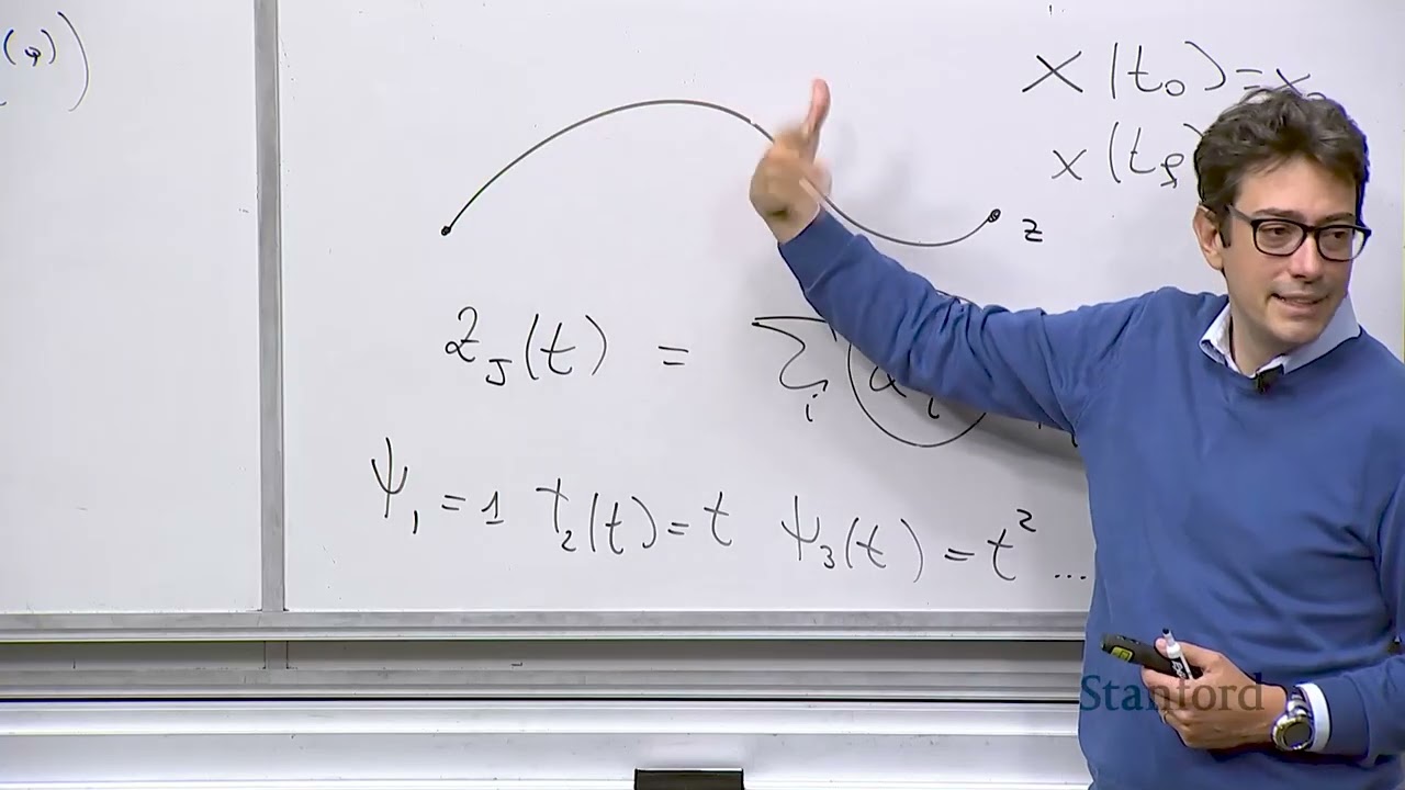
When a robotic system is differentially flat, planning reduces to computing a smooth curve $z(t)$ in the flat output space and running it through the algebraic mappings $\beta$ and $\gamma$. A standard method to construct these curves is polynomial interpolation. Each scalar component $z_j(t)$ of the flat output vector $z(t)$ is parameterized as a linear combination of basis functions:
$$z_j(t) = \sum_{i} \alpha_{ij} \psi_i(t)$$
Common choices for the basis functions $\psi_i(t)$ include canonical polynomial powers ($1, t, t^2, \dots$). The unknown weights $\alpha_{ij}$ are solved by matching boundary conditions at the trajectory endpoints, $x(t_0) = x_0$ and $x(t_f) = x_f$, which map directly to terminal requirements on $z$ and its derivatives.
Prof. Pavone connects this directly to the course problem set, which focuses on an extended unicycle model:
- The system possesses two flat outputs corresponding to planar Cartesian position: $z = [x, y]^T$.
- Fully recovering the unicycle state requires position and velocity information, meaning derivatives $\dot{x}$ and $\dot{y}$ are needed at both boundaries.
- Using a cubic polynomial parameterization yields 4 coefficients per flat output variable, totaling 8 unknown coefficients.
- Evaluating the boundary conditions at $t_0$ and $t_f$ across $x$, $y$, $\dot{x}$, and $\dot{y}$ supplies exactly 8 linear equations, forming a square, solvable linear system that guarantees dynamic feasibility.
- If one wishes to optimize performance rather than merely satisfying boundary constraints, the trajectory can be over-parameterized by selecting higher-degree polynomials (more coefficients than boundary constraints). The remaining degrees of freedom are then resolved by optimizing a secondary objective function, such as minimizing jerk or snap.
---
[08:58](https://www.youtube.com/watch?v=nluc4rMiipA&t=538s) Practical Engineering Workflow and the Physical Meaning of Flat Outputs
Prof. Pavone emphasizes that the underlying mathematics of flatness lead to a pragmatic engineering rule of thumb. Proving that an arbitrary nonlinear system is differentially flat from first principles is notoriously difficult. In practice, roboticists rarely derive flatness proofs from scratch: "What you do is you go on Google Scholar, you type what your system is, and hopefully that system falls in the category of systems that are differentially flat." If the literature confirms it is flat, the engineer can pull the known nonlinear inversion mappings $\beta$ and $\gamma$ and implement the polynomial pipeline directly. With a lighthearted touch, he quips that if the system is not flat, students should simply "call me, and then I give you the lecture slides for AA203," where general non-flat trajectory optimization is covered.
Addressing a student question regarding whether flat outputs are always simply a subset of the full state vector, Prof. Pavone clarifies the mathematical and physical nuances:
- Mathematically, flat outputs in full generality can depend on states, control inputs, and higher-order derivatives of inputs.
- For the extended unicycle model, the flat outputs happen to be a strict coordinate subset of the state space, namely the Cartesian positions $(x, y)$.
- For systems with higher degrees of freedom, such as quadrotors, the flat outputs consist of four coordinates: three-dimensional Cartesian position $(x, y, z)$ alongside the vehicle's yaw heading angle.
- Although mathematical theory allows flat outputs to be complex, abstract algebraic combinations, flat outputs discovered for physical robots almost universally correspond to intuitive physical variables, such as centers of mass, positions, or orientation angles.
[11:36](https://www.youtube.com/watch?v=nluc4rMiipA&t=696s) Addressing Constraints in Differential Flatness
In standard differential flatness trajectory planning, polynomials defining curves in the flat output space $z$ are chosen based primarily on boundary constraints. However, practical robotic systems must satisfy critical physical limitations, notably control input bounds. For a differential-drive robot or unicycle model, the linear driving speed and angular velocity cannot exceed their hardware capabilities:
In course problem sets, for instance, $v_{\max}$ is typically around $0.5\text{ m/s}$. In general, constraints on state $x$ and control $u$ map directly into constraints on the curvature and derivatives of the flat output trajectory. Intuitively, executing sharp corners or sudden turns requires high control effort that can easily saturate actuators.
A student asks whether previous objectives—such as minimizing jerk—already addressed these constraints. Prof. Pavone clarifies that minimizing jerk is carried out directly on the flat output $z$. While optimizing for a smooth profile in flat output space typically produces well-behaved, smooth trajectories in the original state space $x$, this planning stage still operates purely in the flat output space and does not inherently enforce strict hard actuator limits. To handle these bounds without abandoning the computational advantages of differential flatness, an additional tool is required: time scaling.
- **Actuator limits:** Driving speed upper bound $v_{\max}$ (e.g., $0.5\text{ m/s}$ in assignments) and angular rate bound $\omega_{\max}$.
- **Geometric intuition:** High trajectory curvature translates directly into elevated control efforts in the original state-input $(x, u)$ domain.
- **Optimization in flat output space:** Minimizing jerk ensures smoothness, but does not strictly guarantee that input magnitude limits remain satisfied.
---
[14:12](https://www.youtube.com/watch?v=nluc4rMiipA&t=852s) The Core Principle of Time Scaling
Time scaling provides a general and mathematically elegant method for satisfying input bound constraints, not only for wheeled mobile robots but across robotics—most notably in robotic arm manipulator trajectory generation. The central intuition behind time scaling is the explicit decoupling of geometry from timing:
1. **A path:** A purely geometric curve traced in space without any reference to time.
2. **A time schedule:** The rate or timing law dictating how and when the system marches along that path.
To illustrate, consider two runners traversing the exact same spatial path. A fast runner might reach an intermediate checkpoint in 1 second and finish in total time $T$, while a slower runner might reach that same checkpoint in 2 seconds and complete the run in time $2T$. Both follow the identical geometric trajectory, but their pacing differs by a factor of two. By separating path synthesis from pacing, one can first plan a feasible geometric path while disregarding input speed limits, and subsequently synthesize or rescale a timing law $s(t)$ so that the resulting physical velocities and accelerations stay strictly within allowed bounds.
```mermaid
flowchart LR
accTitle: Decoupling Path Geometry from Time Scaling
accDescr: Pipeline showing geometric path generation combined with a monotonic timing law to produce valid bounded trajectories.
subgraph Geometry["Pure Geometry"]
P["Geometric Path<br/>z(s) or θ(s)"]
end
subgraph Timing["Time Law"]
S["Monotonic Timing Law<br/>s(t), with s_dot(t) > 0"]
end
subgraph Execution["Physical Trajectory"]
T["Bounded Trajectory<br/>z(t) = z(s(t))<br/>v(t) = v(s)·s_dot(t) ≤ v_max"]
end
Geometry --> Execution
Timing --> Execution
```
Mathematically, time parameterization is viewed as a composite function $z(t) = z(s(t))$, where $s(t)$ is a continuous scalar time-scaling law satisfying boundary conditions:
$$s(t_0) = s_0, \quad s(t_f) = s_f$$
Crucially, the time scaling must satisfy strict forward progression:
$$\dot{s}(t) > 0$$
This monotonicity property ensures that the robot never moves backward in time as it traverses the trajectory. The geometric curve is commonly parameterized by arc length $s$, representing the physical distance along the path from the origin.
- **Conceptual separation:** Geometric path generation (spatial shape) is solved independently from the time schedule (chronological progression).
- **Monotonicity requirement:** $\dot{s}(t) > 0$ ensures time only moves forward along the curve.
- **Standard parameterization:** Arc length $s$ serves as the natural coordinate for distance along a curve.
---
[18:30](https://www.youtube.com/watch?v=nluc4rMiipA&t=1110s) Time Scaling Example: Manipulator Joint Trajectories
To demonstrate the mechanics concretely, Prof. Pavone presents a standard straight-line interpolation problem for a robotic manipulator with joint angle vector $\theta$. When commanding the arm to transition from an initial joint configuration $\theta_{\text{start}}$ to a final joint configuration $\theta_{\text{end}}$, the path is parameterized using a normalized parameter $s \in [0, 1]$:
$$\theta(s) = \theta_{\text{start}} + s \left(\theta_{\text{end}} - \theta_{\text{start}}\right)$$
At $s = 0$, $\theta(0) = \theta_{\text{start}}$, and at $s = 1$, the expression evaluates exactly to $\theta_{\text{end}}$. A simple timing law to execute this transition over an allocated horizon $T$ is the linear schedule $s(t) = t / T$, which maps $s(0) = 0$ to $s(T) = 1$. Applying the chain rule to compute the joint velocity yields:
Here, total allocated execution time $T$ acts as a direct tuning knob. If joint hardware imposes a maximum angular rate—say, $10\text{ rad/s}$—and the nominal plan exceeds this threshold, increasing $T$ scales down $\dot{\theta}(t)$ by exactly $1/T$ across the entire duration without altering the spatial motion. By stretching total traverse time sufficiently, peak velocities across the trajectory are guaranteed to remain comfortably beneath actuator saturation limits.
- **Manipulator joint path:** $\theta(s) = \theta_{\text{start}} + s(\theta_{\text{end}} - \theta_{\text{start}})$ for $s \in [0, 1]$.
- **Linear time schedule:** $s(t) = \frac{t}{T}$, with derivative $\dot{s}(t) = \frac{1}{T}$.
- **Tuning knob effect:** Increasing the horizon $T$ proportionally decreases the joint velocities $\dot{\theta}$.
---
[21:49](https://www.youtube.com/watch?v=nluc4rMiipA&t=1309s) Scaling Velocities for the Unicycle Model
Extending the formulation to differential flatness, the flat output curve is expressed as $z(t) = z(s(t))$. Taking the time derivative via the chain rule produces:
$$\dot{z}(t) = \frac{dz}{ds} \dot{s}(t)$$
Modulating the time rate $\dot{s}(t)$ scales the derivative $\dot{z}(t)$, allowing control inputs to be capped to their allowable maximums. For a unicycle, the inputs are forward linear velocity $v(t)$ and angular velocity $\omega(t)$. The linear speed is the derivative of position along the curve:
When $s$ represents arc length along the curve $x(s)$, $v(s)$ can be interpreted as the geometric velocity profile along the path as a function of distance from the origin. The true control input $v(t)$ is modulated by multiplying $v(s)$ by the timing rate $\dot{s}(t)$. While linear scaling represents the simplest approach, other parameterizations are common in practice—such as cubic polynomials, which are frequently used in manipulator trajectory profiles to guarantee continuous velocities and accelerations at trajectory boundaries—before evaluating the corresponding angular velocity $\omega(t)$.
- **Chain rule decomposition:** $v(t) = v(s) \dot{s}(t)$, separating path geometry $v(s)$ from time dilation $\dot{s}(t)$.
- **Scaling function choices:** Ranging from simple linear scaling laws ($s(t) = t/T$) to higher-order cubic polynomials ensuring boundary smoothness.
- **Unified framework:** Resolves input saturation for both translational velocity $v(t)$ and heading rate $\omega(t)$ without re-computing the underlying geometric path.
[25:29](https://www.youtube.com/watch?v=nluc4rMiipA&t=1529s) Scaling Velocity and Angular Bounds for the Problem Set
Professor Pavone works through the chain rule relations governing the derivatives along a parameterized path, pausing briefly to check the board notation: "Do you use capital $V$ or small $v$? Yeah, small $v$." Using small $v$, he expresses the time derivative of heading as:
In general trajectory generation, one chooses the time schedule $s(t)$ to guarantee that both the linear velocity bound $v \le v_{\max}$ and the angular velocity bound $\omega \le \omega_{\max}$ are honored. Conceptually, this corresponds to slowing down the traversal along the path until the peak linear speed and peak yaw rate fall within the actuation limits.
```mermaid
flowchart TD
accTitle: Path Scaling Architecture
accDescr: Flowchart illustrating the conversion from geometric path to time-scaled trajectory satisfying actuation bounds.
subgraph GEOM["1. Geometric Parameterization"]
P["Geometric Path x(s)"]
K["Curvature & Heading θ'(s)"]
end
subgraph CONSTR["2. Velocity & Angular Constraints"]
BOUNDS["Input Bounds: v ≤ v_max, ω ≤ ω_max"]
ADJ["Adjust Speed Profile v(s) or Schedule s(t)"]
end
subgraph TRAJ["3. Executable Trajectory"]
NOM["Time-Parameterized Reference: x_d(t), u_d(t)"]
end
P --> K
K --> ADJ
BOUNDS --> ADJ
ADJ --> NOM
```
Pavone highlights a deliberate tweak designed for the first assignment: "That is like a twist that I made for the P set to make it more engaging, but it's useful." Rather than defining an explicit time scaling law $s(t)$ directly, students in Problem Set 1 readjust the velocity along the arc length parameterization, directly tuning $v(s)$ such that $v(s) \le v_{\max}$ and $\omega(s) \le \omega_{\max}$. Modifying the velocity profile along the fixed geometric path implicitly dictates a new time schedule, because arrival time at any spatial coordinate is simply the integral of slowness (reciprocal velocity) with respect to arc length:
$$t(s) = \int \frac{1}{v(s)} \, ds$$
When a student points out that adjusting the speed profile $v(s)$ directly feels more natural, Pavone readily agrees: "Once you get a hang of it, then it's more natural... It's a much more direct way." He explains that presenting explicit time scaling laws $s(t)$ first is chosen primarily for pedagogical clarity when introducing the mechanics of decoupling geometry from time.
- General time scaling: slow down $s(t)$ until maximum $v$ and maximum $\omega$ remain strictly below physical thresholds.
- Problem Set 1, Problem 1 twist: keep the geometric path fixed, recompute the arc length velocity profile $v(s)$ directly to satisfy constraints, implicitly generating the revised timing law.
---
[29:20](https://www.youtube.com/watch?v=nluc4rMiipA&t=1760s) Clarifying the Composition: $x(s(t))$ and Arc Length Parameterization
A student asks whether the path composition should be written as $x(s(t))$ or $x(t(s))$, wondering if differentiating with respect to arc length implies that time is an inverted function of space. Pavone clarifies the mathematical interpretation: time $t$ remains the fundamental independent variable. The configuration is modeled as $x(s(t))$, viewing position in space as depending indirectly on time via the intermediate arc length variable $s$. At any given instant $t$, the schedule reveals where the robot lies along the path, $s(t)$, and the geometric map $x(s)$ returns the corresponding Cartesian state.
$$\text{Time } t \;\xrightarrow{\quad s(t)\quad}\; \text{Arc Length } s \;\xrightarrow{\quad x(s)\quad}\; \text{State } x(s(t))$$
Inverting this dependency to $x(t(s))$ would make arc length $s$ the independent driving variable, which would reverse the application of the chain rule. Pavone cautions that while the concept appears straightforward on paper, "it's deceptively simple" and requires careful attention when deriving derivatives.
He then defines the parameters of the time-scaling function:
- $t$: the current running time variable.
- $T$: the total allocated traversal horizon, which is tuned so the robot meets the control limits without running arbitrarily slowly.
- $L$: the total geometric length of the path, satisfying the terminal condition $s(T) = L$.
When asked whether alternative parameterizations exist aside from arc length, Pavone calls arc length the "de facto standard." It cleanly isolates pure path geometry from temporal progression, letting an engineer pick desired velocities point-by-point along the curve while automatically preserving kinematic consistency.
---
[33:18](https://www.youtube.com/watch?v=nluc4rMiipA&t=1998s) Transitioning from Open-Loop Planning to Closed-Loop Tracking
Pavone reviews the broader two-step control architecture introduced in earlier lectures:
1. **Open-Loop Trajectory Computation:** Differential flatness yields nominal state trajectories $x_d(t)$ and open-loop control feeds $u_d(t)$ through the differential equations of motion, followed by time scaling to satisfy actuator saturation bounds.
2. **Closed-Loop Trajectory Tracking:** An auxiliary feedback controller runs in tandem with the feedforward commands to reject disturbances and correct for model mismatches.
Pavone stresses that relying purely on open-loop execution is fragile: in the real world, errors accumulate rapidly without a feedback mechanism constantly measuring performance and adjusting commands. Consequently, the nominal feedforward plan must be wrapped in a closed-loop tracking controller designed to operate locally within a bounding envelope ("a cube") around the desired nominal trajectory $x_d(t)$ (where the subscript $d$ denotes *desired*). In terms of course logistics, computing the open-loop trajectory corresponds to Problem 1 in the problem set, while designing the tracking controller corresponds to Problem 3.
```mermaid
flowchart LR
accTitle: Two-Step Trajectory Tracking Architecture
accDescr: Block diagram showing desired trajectory feeding forward while feedback error drives tracking control.
subgraph OPENLOOP["Feedforward Planning"]
REF["Trajectory Generator (Flatness + Scaling)"]
end
subgraph CLOSEDLOOP["Feedback Tracking"]
CTRL["Tracking Controller"]
ROBOT["Robot Dynamics"]
SUM(( +))
end
REF -->|"x_d(t)"| CTRL
REF -->|"u_d(t)"| SUM
CTRL -->|"δu(t)"| SUM
SUM -->|"u(t)"| ROBOT
ROBOT -->|"x(t)"| CTRL
```
---
[35:15](https://www.youtube.com/watch?v=nluc4rMiipA&t=2115s) Tracking Control Strategies: Pure Pursuit and Linearization
Trajectory tracking centers on synthesizing a control law that evaluates the error between the robot's current state $x(t)$ and the target state $x_d(t)$, mapping that deviation into corrective inputs. Pavone outlines the primary methodologies used to design these controllers:
1. **Geometric Pursuit Control:** The simplest practical approach is purely geometric, often referred to as pursuit control. Instead of aiming directly at the instantaneous reference point $x_d(t)$, the controller establishes a lookahead target along the trajectory—for instance, a point $\Delta t$ seconds ahead (such as $t + \Delta t$, or roughly two seconds down the path). The controller then steers the robot directly toward this lookahead intercept point along a simple geometric line. Pavone compares the mechanism to a classic visual metaphor: "It's like a donkey that is chasing the carrot. That is an example of, if you will, tracking. Here, this is the carrot... It is moving along the path and is always, say, two seconds away along the path, and you're always trying to aim at that point." A student asks whether the carrot point requires matching the path's tangent at that location, and Pavone clarifies that it does not—the vehicle simply points directly toward the moving intercept point. Despite its intuitive simplicity, pure pursuit controllers are widely deployed and perform remarkably well in practice.
2. **Linearization-Based Control:** The second major family of tracking approaches relies on linearizing the nonlinear dynamics to leverage the extensive toolkit of linear control theory. As Pavone notes, linear control is substantially easier, better understood, and more tractable than nonlinear control. System linearization splits into two distinct paradigms:
- *Exact Linearization (Feedback Linearization):* A technique intimately connected to differential flatness that uses mathematical transformations and state feedback to cancel out nonlinearities entirely.
- *Approximate (Jacobian) Linearization:* Expanding the system dynamics via a Taylor series around the reference trajectory to govern small perturbations.
[037:50] Alternatives for Trajectory Tracking: Inexact Linearization, Nonlinear Control, and MPC
Prof. Marco Pavone resumes the overview of candidate strategies for trajectory tracking by presenting the second alternative: *inexact linearization*. In typical trajectory tracking scenarios, assuming nothing catastrophic occurs, the robot remains very close to its nominal reference trajectory. Because deviations are small and local, any nonlinear function can be approximated near that nominal operating point by a straight line—its first-order Taylor series approximation. Once linearized, engineers can deploy well-established linear control methods. While intuitive for anyone with a background in control systems, it can feel somewhat obscure to newcomers, but it represents a widespread practical option.
```mermaid
flowchart TD
accTitle: Trajectory Tracking Methodologies
accDescr: High-level overview of four candidate approaches for trajectory tracking control design.
B -->|"Pros: Standard linear tools<br/>Cons: Only locally valid"| ResB["Local Linear Models"]
C -->|"Pros: No approximations<br/>Cons: Very difficult analytically"| ResC["Direct Nonlinear Laws"]
D -->|"Pros: Handles constraints<br/>Cons: Beyond course scope"| ResD["Online Optimization"]
A -->|"Course Focus: Pedagogical,<br/>exact, widely practical"| ResA["Global / Equivalent Linear Models"]
```
The third alternative is *nonlinear control techniques*, where one tackles the differential equations directly without making local approximations or strange transformations. Although appealing in principle because no modeling simplifications are made, in practice this approach is mathematically daunting and rarely yields tractable closed-form solutions. The fourth methodology centers on *optimization-based control*, most notably Model Predictive Control (MPC). In MPC, finding the control action at each time step requires solving an online optimization problem. While MPC handles diverse constraints exceptionally well, it is beyond the scope of AA274A. Pavone reiterates the class philosophy: survey the broad landscape of available methods, then dive deeply into one pedagogically rich and practically vital approach—namely, exact linearization via differential flatness.
- **Inexact Linearization**: Truncates the system's Taylor series expansion to produce a locally valid linear model around the nominal path.
- **Direct Nonlinear Control**: Avoids approximations, but exact closed-form control designs are often mathematically intractable.
- **Optimization-Based Control (MPC)**: Converts control into an online constrained optimization problem; powerful, but deferred to more advanced coursework.
- **Pedagogical Selection**: The lecture focuses entirely on exact linearization grounded in differential flatness due to its balance of mathematical elegance and widespread robotics adoption.
---
[040:25] The Mechanics of Exact Linearization and Virtual Control Inputs
Pavone pivots to the deep dive into exact linearization. For certain systems—specifically, differentially flat systems—one can execute a nonlinear change of coordinates alongside an input transformation that maps the original nonlinear system bijectively into an equivalent linear system. Because the mapping is one-to-one, solutions to the linear representation map directly back to the original nonlinear dynamics. Consequently, one can design a controller using linear methods for the transformed system and pull it back to recover the nonlinear physical control inputs.
To illustrate how effortless this idea can be, Pavone walks through an elementary scalar example:
$$\dot{x} = f(x) + u$$
If tasked with driving $x$ to the origin, one might dread the nonlinear function $f(x)$ because solving the differential equation analytically is hard. However, one can define a *virtual control input* $v$:
$$f(x) + u = v \implies \dot{x} = v$$
Designing $v$ to drive $x \to 0$ with an arbitrary rate of exponential convergence is trivial since it is the simplest possible linear differential equation. Once $v$ is determined, the actual control input $u$ fed to the physical plant is recovered by inverting the algebraic relation:
$$u = v - f(x)$$
This calculation directly cancels the internal nonlinearity $f(x)$ and replaces the system's behavior with an engineered linear response. Pavone emphasizes why this is called *exact* linearization: unlike inexact methods, no Taylor series truncation or local approximation occurs. The cancellation is globally exact—provided the system belongs to the class of differentially flat systems.
```mermaid
flowchart LR
accTitle: Virtual Input and Exact Linearization Concept
accDescr: Pipeline showing how a virtual control input cancels system nonlinearities to create linear error dynamics.
subgraph Execution["Control Synthesis and Inversion"]
direction TB
C1["Design Linear Control v<br/>(e.g., v = -k*x)"]
C2["Invert Mapping:<br/>u = v - f(x)"]
C3["Apply physical control u<br/>to actual system"]
C1 --> C2 --> C3
end
Transformation --> Execution
```
- **Core Mechanism**: Introduce a virtual input $v$ such that nonlinear terms cancel algebraically, producing linear synthetic dynamics.
- **Global Validity**: No truncation of high-order Taylor terms; the system is transformed exactly without local degradation.
- **Theoretical Backbone**: Differential flatness guarantees that every flat system can be equivalently cast into a linear system driven by higher-order derivatives of the flat output.
- **Reference**: Pavone points students interested in deeper theoretical proofs to literature such as Meyn and Scherer (2009).
---
[044:33] Tracking Control Design in Flat Output Space
Having established that a differentially flat system maps into a linear chain of integrators, Pavone details the tracking controller architecture. Let $z(t)$ denote the actual flat output vector achieved by the physical vehicle (subject to disturbances and model imperfections), and let $z_d(t)$ be the desired nominal trajectory. For the $i$-th component of the flat output, the tracking error signal is defined as:
$$e_i(t) = z_i(t) - z_{i,d}(t)$$
Because the flat output dynamics obey a chain of integrators up to derivative order $q+1$, taking the $(q+1)$-th time derivative of the error yields:
$$e_i^{(q+1)}(t) = z_i^{(q+1)}(t) - z_{i,d}^{(q+1)}(t) = w_i(t) - w_{i,d}(t)$$
where $w_i(t)$ is the virtual control input for coordinate $i$, and $w_{i,d}(t) = z_{i,d}^{(q+1)}(t)$ is the feedforward control corresponding to the reference trajectory.
To drive this error to zero, one chooses the virtual control input $w_i(t)$ to cancel the feedforward requirement and superimpose stable linear error feedback:
$$w_i(t) = w_{i,d}(t) - \sum_{j=0}^{q} K_{i,j} \, e_i^{(j)}(t)$$
Substituting this feedback law back into the $(q+1)$-th derivative expression yields the closed-loop error differential equation:
$$e_i^{(q+1)}(t) + \sum_{j=0}^{q} K_{i,j} \, e_i^{(j)}(t) = 0$$
This is a standard homogeneous linear ordinary differential equation with constant coefficients $K_{i,j}$. As Pavone explains, designing the tracking controller boils down to selecting the gains $K_{i,j}$ such that the characteristic polynomial has all its roots (eigenvalues) strictly in the open left half-plane (negative real parts). When that condition holds, the error $e_i(t)$ and all of its derivatives up to order $q$ converge asymptotically to zero, guaranteeing that the true system output tracks the nominal reference path.
- **Feedforward Component**: $w_{i,d}(t)$ provides the nominal input needed to follow the prescribed trajectory smoothly.
- **Feedback Compensation**: Linear gain terms $K_{i,j} \, e_i^{(j)}(t)$ act on tracking errors across position and higher-order derivatives (velocity, acceleration, etc.).
- **Pole Placement**: Controller tuning reduces to classical eigenvalue assignment ensuring negative real parts for asymptotic stability.
- **Role of $q$**: Parameter $q$ reflects the highest derivative order of the inputs and states needed to represent the flat output space. Pavone notes that determining whether an arbitrary system is differentially flat remains an inherently difficult theoretical question.
[50:27](https://www.youtube.com/watch?v=nluc4rMiipA&t=3027s) The Challenge of Finding Flat Outputs and the Extended Unicycle Model
Finding the transformation that proves a system is differentially flat is inherently difficult. A priori, nobody tells an engineer how many derivatives of the input must be considered to uncover the mapping. While some automated procedures exist, they do not scale well. In practice, researchers begin by testing whether a one-to-one mapping exists without including the input $u$, before iteratively adding higher derivatives. As Professor Pavone emphasizes, finding that a useful physical system is differentially flat is significant enough that researchers "usually write a paper about it because usually it entailed a lot of work."
To ground these abstract mathematical concepts, the lecture turns to the extended unicycle model. This model is chosen because it serves as an excellent pedagogical tool, is practically useful, and appears directly on the problem set. The model extends the standard kinematic unicycle by adding an integrator on the linear velocity $V$:
$$\dot{V} = a$$
Rather than treating velocity directly as an input, the actual control inputs are acceleration $a$ and angular velocity $\omega$, providing a much more realistic physical representation of a mobile robot.
[51:42](https://www.youtube.com/watch?v=nluc4rMiipA&t=3102s) Feedback Linearization via Flat Outputs
The extended unicycle system is differentially flat with flat outputs chosen as the Cartesian coordinates $(x, y)$. Differentiating the position coordinates with respect to time yields:
$$\dot{x} = V \cos\theta, \quad \dot{y} = V \sin\theta$$
Taking the second time derivatives of the flat outputs produces:
$$\ddot{x} = \dot{V}\cos\theta - V\sin\theta\,\dot{\theta}$$
$$\ddot{y} = \dot{V}\sin\theta + V\cos\theta\,\dot{\theta}$$
Substituting the system dynamics ($\dot{V} = a$ and $\dot{\theta} = \omega$) allows this relationship to be written in matrix form:
$$\begin{bmatrix} \ddot{x} \\ \ddot{y} \end{bmatrix} = \begin{bmatrix} \cos\theta & -V\sin\theta \\ \sin\theta & V\cos\theta \end{bmatrix} \begin{bmatrix} a \\ \omega \end{bmatrix} = J \begin{bmatrix} a \\ \omega \end{bmatrix}$$
Defining a virtual control input vector $\begin{bmatrix} u_1 \\ u_2 \end{bmatrix}$ equivalent to $\begin{bmatrix} \ddot{x} \\ \ddot{y} \end{bmatrix}$, the nonlinear kinematics collapse into a simple linear double-integrator system:
$$\ddot{x} = u_1, \quad \ddot{y} = u_2$$
```mermaid
flowchart LR
accTitle: Feedback Linearization for the Extended Unicycle
accDescr: Diagram illustrating how virtual control inputs are transformed through matrix inversion to physical inputs.
subgraph LinearControl["Linear Control Domain"]
U["Virtual Inputs (u₁, u₂)"]
end
subgraph Decoupling["Inversion Mapping"]
InvJ["J⁻¹(θ, V)"]
end
subgraph PhysicalInputs["Physical Robot Domain"]
Actual["Inputs (a, ω)"]
Robot["Extended Unicycle Dynamics"]
Outputs["Flat Outputs (x, y)"]
end
U --> InvJ
InvJ --> Actual
Actual --> Robot
Robot --> Outputs
```
To recover the physical control inputs $(a, \omega)$, the decoupling matrix $J$ must be inverted:
$$\begin{bmatrix} a \\ \omega \end{bmatrix} = J^{-1} \begin{bmatrix} u_1 \\ u_2 \end{bmatrix}$$
Calculating the determinant of $J$ gives:
$$\det(J) = V\cos^2\theta - (-V\sin^2\theta) = V(\cos^2\theta + \sin^2\theta) = V$$
When $V = 0$, the matrix becomes singular and the transformation breaks down. Differential flatness often introduces such points of singularity. In advanced literature, singularities are handled by prolonging the mappings to keep them well-defined everywhere. In this course, a simpler and pragmatic engineering heuristic is used: if the velocity falls below a small threshold (e.g., $10^{-4}$ or $10^{-5}$), it is clamped to that floor value to prevent numerical blowup during matrix inversion.
[54:49](https://www.youtube.com/watch?v=nluc4rMiipA&t=3289s) Linear Tracking Controller and Closed-Loop Error Dynamics
With the system linearized via feedback, tracking control reduces to stabilizing the tracking error independently along each flat output coordinate. For the $x$-coordinate, the virtual control input $u_1 = \ddot{x}$ is defined using feedforward and feedback gains:
$$\ddot{x} = \ddot{x}_d + k_{d,x}(\dot{x}_d - \dot{x}) + k_{p,x}(x_d - x)$$
where $x_d(t)$, $\dot{x}_d(t)$, and $\ddot{x}_d(t)$ denote the desired trajectory and its time derivatives.
Defining the tracking error as $e_x = x - x_d$, the closed-loop error equation rearranges into a standard second-order linear differential equation:
$$\ddot{e}_x + k_{d,x}\dot{e}_x + k_{p,x}e_x = 0$$
- By Descartes' rule of signs, choosing positive gains ($k_{p,x} > 0$ and $k_{d,x} > 0$) guarantees that the roots of the characteristic polynomial have strictly negative real parts, rendering the error dynamics asymptotically stable ($e_x \to 0$ as $t \to \infty$).
- Although arbitrarily high gains drive tracking errors to zero faster in theory, in practice aggressive gains cause actuator saturation. If actuator limits are exceeded, the reference trajectory must be time-scaled to keep required inputs within bounds.
- The overarching power of differential flatness is that open-loop trajectory generation (via path planning plus time scaling) and closed-loop trajectory tracking design are unified cleanly within the same mathematical framework.
[59:49](https://www.youtube.com/watch?v=nluc4rMiipA&t=3589s) Generalized Coordinates and Reference Trajectory Workflow
In response to student questions about the general notation, the abstract variables are mapped back to the unicycle example:
- The generalized state vector $z^{(q+1)}$ corresponds to the highest derivative of the flat outputs, which is $\begin{bmatrix} \ddot{x} & \ddot{y} \end{bmatrix}^T$ (here $q = 1$).
- The generalized input $w$ corresponds to the virtual inputs $\begin{bmatrix} u_1 & u_2 \end{bmatrix}^T$.
Addressing a student's question on whether the underlying mathematical derivations must be re-derived from scratch, Professor Pavone reassures the class that from a practitioner's perspective, one rarely needs to construct the deep differential algebraic proofs. Instead, engineers identify whether their system has been established as differentially flat in the robotics literature, locate the published mappings, and employ the resulting feedforward and feedback equations.
Finally, clarifying where the desired reference trajectory $x_d(t)$ originates, the professor outlines the end-to-end control workflow:
1. **Open-Loop Design**: An open-loop reference input $u_d(t)$ and state trajectory $x_d(t)$ are planned using differential flatness and time scaling.
2. **Trajectory Feedforward and Feedback**: The overall control command combines the desired feedforward terms with the feedback corrections operating on tracking errors $(x_d - x)$ and $(\dot{x}_d - \dot{x})$.
3. **Physical Command Computation**: The resulting virtual linear controls are mapped through the nonlinear inversion transformation (matrix $J^{-1}$) to produce the physical actuation commands $(a, \omega)$ sent to the robot hardware.
[01:03:37](https://www.youtube.com/watch?v=nluc4rMiipA&t=3817s) Tracking Controllers, Error Derivatives, and Gain Tuning
Concluding the discussion on tracking controllers, the controller naturally depends on the desired open-loop trajectory, as that is the exact reference path the robot seeks to follow. A student raises a question regarding the feedback policy $\pi$ discussed on the preceding slide, asking whether $\pi$ also depends on the error derivative $\dot{x}(t) - \dot{x}_{\text{ref}}(t)$. The instructor confirms that it does; using the state trajectory history requires consistent estimation or direct measurement of the velocity $\dot{x}$ and acceleration $\ddot{x}$ states to construct the error derivatives.
Another student questions why the feedback control gains must be strictly positive and whether that condition directly guarantees that the closed-loop system eigenvalues remain stable in the left-half complex plane. The instructor affirms this, noting that Descartes' Rule of Signs explains why positive coefficients yield negative real roots for the characteristic polynomial. He clarifies standard control notation:
- $k_P$ denotes the **proportional** gain (scaling the state error directly).
- $k_D$ denotes the **derivative** gain (scaling the rate of change of state error, where "D" stands for derivative, not desired).
- Integral action ($k_I$) is often appended in full PID implementations, though here the focus remains on PD action.
---
[01:05:31](https://www.youtube.com/watch?v=nluc4rMiipA&t=3931s) Closed-Loop Control: Optimal Control vs. Lyapunov Analysis
Transitioning from the standard two-step design (open-loop planning followed by local tracking), the lecture shifts to the global perspective of closed-loop control. The "holy grail" of trajectory planning and control is finding a global feedback law $\pi(x)$ that is valid everywhere across the entire state space, rather than merely within a narrow tube around a precomputed nominal trajectory. Such a policy guarantees that regardless of modeling errors, massive disturbances, or external drift pushing the robot far off course, the controller instantly dictates the exact corrective action required to reach the goal.
```mermaid
flowchart TD
accTitle: Approaches to Closed Loop Control
accDescr: Comparison between Hamilton-Jacobi-Bellman optimization and Lyapunov stability analysis.
subgraph GlobalControl["Global Closed-Loop Control Methods"]
HJB["Hamilton-Jacobi-Bellman (HJB) / Dynamic Programming"]
LYAP["Lyapunov Stability Analysis"]
end
Because computing these global policies everywhere is computationally intractable for complex systems, the two-step design remains the standard engineering trade-off. Historically, two primary frameworks address global closed-loop design:
- **Hamilton-Jacobi-Bellman (HJB) Equation**: Solves general nonlinear continuous-time optimal control problems. The resulting partial differential equation (PDE) suffers from the curse of dimensionality and is rarely solvable in closed form. Its discrete-time counterpart is **Dynamic Programming**, foundational in reinforcement learning and stochastic optimal control (covered in advanced courses like AA 203). This paradigm solves for both feasibility and cost minimization (optimality).
- **Lyapunov Analysis**: Focuses on task fulfillment and asymptotic stabilization (steering states to an equilibrium) without necessarily minimizing an objective cost function. It primarily addresses feasibility rather than optimality (covered in nonlinear control courses such as ENGR 209).
---
[01:08:44](https://www.youtube.com/watch?v=nluc4rMiipA&t=4124s) Unicycle Posture Regulation in Polar Coordinates
To illustrate closed-loop stabilization concretely, the instructor turns to posture regulation for the standard nonholonomic unicycle model. The control inputs remain the linear forward speed $v$ and angular velocity $\omega$, acting on Cartesian states $(x, y)$ and heading $\theta$. The objective is to stabilize the robot to rest at the origin $(x=0, y=0, \theta=0)$ from arbitrary initial states across the plane.
```mermaid
flowchart LR
accTitle: Coordinate Transformation for Unicycle Stabilization
accDescr: Transformation from Cartesian states x, y, theta to polar coordinates rho, alpha, delta.
subgraph Cartesian["Cartesian Frame"]
CState["(x, y, θ)"]
end
subgraph Polar["Polar Frame"]
PState["(ρ, α, δ)"]
end
CState -->|"Nonlinear Transformation"| PState
```
Carrying out the analysis directly in Cartesian coordinates is algebraically awkward, so the system is transformed into a polar coordinate representation $(\rho, \alpha, \delta)$:
- $\rho = \sqrt{x^2 + y^2}$: The Euclidean distance from the unicycle reference point to the origin.
- $\delta$: The angular coordinate representing the orientation of the line-of-sight vector with respect to the global reference frame.
- $\alpha$: The heading error between the unicycle's current orientation and the line of sight pointing directly toward the origin.
The transformation provides clear physical intuition into the unicycle's kinematics:
- The rate of change of distance, $\dot{\rho}$, depends purely on the forward linear velocity $v$ and the pointing alignment $\cos(\alpha)$; rotating purely in place ($v = 0, \omega \neq 0$) changes vehicle orientation but leaves the distance $\rho$ unchanged.
- When $\alpha = 0$, heading points directly toward the target, maximizing the rate of approach $|\dot{\rho}|$. When $\alpha = \pm \frac{\pi}{2}$, the unicycle travels tangentially in a circle relative to the origin, resulting in $\dot{\rho} = 0$.
- The line-of-sight angle rate $\dot{\delta}$ depends on $v$, whereas the heading error rate $\dot{\alpha}$ depends on both $v$ and the steering input $\omega$.
By formulating inputs $v(\rho, \alpha, \delta)$ and $\omega(\rho, \alpha, \delta)$ as nonlinear functions of these polar states, one constructs a closed-loop policy that provably guarantees asymptotic convergence to the origin from all starting configurations—a result students prove directly in homework problem sets.
[01:13:43](https://www.youtube.com/watch?v=nluc4rMiipA&t=4423s) Lyapunov Analysis and Feedback Control Law Foundations
To build intuition for how stabilizing feedback control laws are synthesized, Professor Pavone outlines the classical framework of Lyapunov analysis. He reassures the class that this discussion is strictly conceptual to ensure completeness: students will not be asked to derive nonlinear Lyapunov control laws on their midterms. The core mechanism relies on postulating a candidate Lyapunov function, typically denoted $V$, representing an abstract "energy" of the system. This function is chosen to be positive definite—resembling a bowl—and evaluates to zero strictly at the desired equilibrium point (the origin).
If a control law can steer the state along the level sets of this Lyapunov function such that the value of $V$ strictly decreases over time, the system is mathematically guaranteed to converge asymptotically to the origin. In practice, the designer computes the analytical time derivative of the postulated energy function, $\dot{V}$, and then algebraically selects control inputs that enforce $\dot{V} < 0$ for all non-zero states. Applying this methodology produces an explicit, globally stabilizing closed-loop control law.
From any initial condition, this law computes instantaneous steering commands that will drive the robot to the goal. While the resulting paths are dynamically feasible, Pavone notes with a grin that the trajectories can sometimes look unusual: "You may like it, you may not like it. It's feasible. Sometimes it does something weird." Nonetheless, stability and convergence to the origin are mathematically guaranteed from any starting configuration, a property students verify empirically through numerical experiments in their problem set.
- **Lyapunov function properties**: Postulated positive-definite energy function $V(x)$ shaped like a bowl, where $V(0) = 0$ and $V(x) > 0$ for all $x \neq 0$.
- **Control law design condition**: Inputs are chosen analytically to force the time derivative $\dot{V} < 0$, guaranteeing descent toward the origin.
- **Midterm expectations**: Students are not required to derive Lyapunov control laws on the midterm exam; the topic is introduced for algorithmic context and mathematical intuition.
---
[01:15:26](https://www.youtube.com/watch?v=nluc4rMiipA&t=4526s) Terminal Guidance: Combining Two-Step Design with Fast Posture Control
Although the standard two-step design framework—generating an open-loop nominal trajectory followed by a trajectory-tracking feedback controller—appears complete on paper, standalone closed-loop control laws remain indispensable in practical robotics. The primary challenge arises in terminal guidance: as the vehicle approaches within close proximity of its goal, running computationally heavy trajectory updates can become a bottleneck. Under close-range terminal conditions, the robot requires a controller that closes the loop at high frequencies in an exceptionally robust, dependable manner.
A closed-loop posture controller achieves this responsiveness because it bypasses numerical optimization entirely. Instead of solving constrained mathematical programs or iterative algebraic systems online, the controller directly reads the current polar-coordinate error states—the distance to target $\rho$, heading angle $\alpha$, and target offset angle $\delta$—and evaluates basic trigonometric functions ($\sin$ and $\cos$) to instantly compute the velocity inputs. To illustrate, Pavone shares a concrete aerospace application from his own research: operating a robotic platform deployed aboard the International Space Station tasked with capturing objects floating in microgravity. Far from the target, the robot follows a planned trajectory from a two-step design. Once it gets right next to the tumbling target, it switches over to a fast closed-loop posture control law. Because the vehicle is already in the immediate vicinity, obstacle constraints can be safely neglected, allowing the high-rate reactive loop to deliver the tight real-time coordination necessary for grasping and manipulation.
```mermaid
flowchart TD
accTitle: Hybrid Terminal Guidance Pipeline
accDescr: Diagram illustrating the switch from coarse two-step planning at long range to reactive posture control at terminal range.
subgraph FarRange["Far-Range Navigation"]
A["Global Motion Planner"] -->|"Nominal Path"| B["Two-Step Trajectory Tracking"]
B -->|"Considers State Constraints"| C{"Distance to Target"}
end
subgraph TerminalRange["Close-Range Manipulation"]
C -->|"rho <= Threshold"| D["Reactive Posture Controller"]
D -->|"Evaluates Closed-Form Trig"| E["Ultra-Fast Actuation"]
end
```
- **Computational simplicity**: Closed-form posture control avoids real-time optimization, operating purely on direct state evaluations of $\rho$, $\alpha$, and $\delta$.
- **Aerospace deployment example**: Robots aboard the International Space Station utilize two-step trajectory tracking for long-range approach, transitioning to pure feedback control laws for high-speed terminal grasping.
- **Constraint handling trade-off**: Terminal posture controllers ignore complex state constraints, which is acceptable within a small, cleared neighborhood surrounding the target.
---
[01:17:00](https://www.youtube.com/watch?v=nluc4rMiipA&t=4620s) Course Roadmap: Problem Set 2 and Advanced Optimal Control Preview
Pavone explains how these conceptual components coalesce across the course assignments. In Problem Set 2, students construct an integrated, end-to-end trajectory pipeline. They take the foundational two-step controller engineered in Problem Set 1 and augment it with an explicit motion planning module capable of navigating around obstacles and satisfying environmental state constraints—limitations that had not been incorporated into the earlier tracking formulations. Finally, they layer the closed-loop posture controller onto the pipeline as a robust terminal docking phase. Combining global planning, nominal feedforward generation, local tracking, and terminal posture stabilization provides the architecture required for the course's final autonomous driving project.
Before adjourning, Pavone previews the upcoming lecture. The Friday session introduces advanced optimal control and trajectory optimization, focusing on indirect methods such as Pontryagin's Minimum Principle and calculus of variations. Attendance for the Friday lecture is mandatory for graduate students enrolled in the class, while remaining optional for undergraduates, before the full cohort reconvenes for standard lectures the following Tuesday.
- **Problem Set 2 architecture**: Blends global motion planning for obstacle avoidance, two-step trajectory tracking, and terminal posture control into an end-to-end framework.
- **Final project application**: The multi-tier architecture forms the foundational navigation stack utilized by students in their capstone autonomous vehicle project.
- **Next lecture focus**: Advanced optimal control techniques, specifically contrasting direct optimization with indirect methods. Attendance is required for graduate students and optional for undergraduate students.
## Notable quotes
> [08:58](https://www.youtube.com/watch?v=nluc4rMiipA&t=538s) What you do is you go on Google Scholar, you type what your system is, and hopefully that system falls in the category of systems that are differentially flat. — Prof. Marco Pavone
> [08:58](https://www.youtube.com/watch?v=nluc4rMiipA&t=538s) call me, and then I give you the lecture slides for AA203 — Prof. Marco Pavone
> [25:29](https://www.youtube.com/watch?v=nluc4rMiipA&t=1529s) Do you use capital V or small v? Yeah, small v. — Prof. Marco Pavone
> [25:29](https://www.youtube.com/watch?v=nluc4rMiipA&t=1529s) That is like a twist that I made for the P set to make it more engaging, but it's useful. — Prof. Marco Pavone
> [25:29](https://www.youtube.com/watch?v=nluc4rMiipA&t=1529s) Once you get a hang of it, then it's more natural... It's a much more direct way. — Prof. Marco Pavone
> [29:20](https://www.youtube.com/watch?v=nluc4rMiipA&t=1760s) it's deceptively simple — Prof. Marco Pavone
> [35:15](https://www.youtube.com/watch?v=nluc4rMiipA&t=2115s) It's like a donkey that is chasing the carrot. That is an example of, if you will, tracking. Here, this is the carrot... It is moving along the path and is always, say, two seconds away along the path, and you're always trying to aim at that point. — Prof. Marco Pavone
> [50:27](https://www.youtube.com/watch?v=nluc4rMiipA&t=3027s) usually write a paper about it because usually it entailed a lot of work. — Prof. Marco Pavone
> [01:13:43](https://www.youtube.com/watch?v=nluc4rMiipA&t=4423s) You may like it, you may not like it. It's feasible. Sometimes it does something weird. — Prof. Marco Pavone
## Mentioned
Marco Pavone, Stanford University, AA274A, AA203, Google Scholar, Meyn and Scherer (2009), Descartes' rule of signs, Hamilton-Jacobi-Bellman (HJB), International Space Station, Pontryagin's Minimum Principle
## Video description
For more information about Stanford’s graduate programs, visit: https://online.stanford.edu/graduate-education
Lecture 4 — Trajectory Tracking and Closed-Loop Control
Note: This lecture was recorded as part of the 2019 edition of the course. Course content, structure, assignments, and other materials may have changed since this recording. The course links below point to the most recent edition and may therefore differ from what is presented in the video.
Read the companion textbook, Principles of Robot Autonomy, free online: https://porabook.com
Follow along with the latest course schedule and syllabus: https://stanfordasl.github.io/PoRA-I
Speaker: Prof. Marco Pavone
Dr. Marco Pavone is an Associate Professor of Aeronautics and Astronautics at Stanford University and a Senior Director of Autonomous Vehicle Research at NVIDIA. Prior to joining Stanford, he was a Research Technologist in the Robotics Section at NASA’s Jet Propulsion Laboratory. Dr. Pavone received his Ph.D. in Aeronautics and Astronautics from the Massachusetts Institute of Technology in 2010. His research focuses on the analysis, design, and control of autonomous systems, with particular emphasis on self-driving cars, autonomous aerospace vehicles, and future mobility systems. He has been recognized with numerous awards, including the Presidential Early Career Award for Scientists and Engineers from President Barack Obama, the Office of Naval Research Young Investigator Award, the NSF CAREER Award, the NASA Early Career Faculty Award, the IEEE Kiyo Tomiyasu Award, the CSS Award for Technical Excellence in Aerospace Control, and the Early-Career Spotlight Award from the Robotics Science and Systems Foundation.
Instructor:
Prof. Marco Pavone, Associate Professor of Aeronautics and Astronautics, Director of Autonomous Vehicle Research at NVIDIA
Full playlist: https://www.youtube.com/playlist?list=PLR9iNyexfIkk
Prof. Marco Pavone presents a robotic trajectory architecture that combines open-loop differential flatness and time scaling with closed-loop feedback linearization and terminal posture stabilization.
Differential Flatness for Rapid Trajectory Synthesis (3:14)
In many practical robotics applications, finding an optimal trajectory via computationally heavy direct or indirect methods is unnecessary if a feasible trajectory can be generated rapidly. Differential flatness resolves this by establishing a bijective mapping between trajectories in a lower-dimensional flat output space and dynamically feasible state-input pairs. Because states and inputs can be algebraically reconstructed without numerically integrating differential equations, dynamic constraints are effectively eliminated.
For systems such as the extended unicycle model, the flat outputs map directly to Cartesian position coordinates $(x, y)$. Engineers can parameterize trajectories using polynomial interpolation, resolving unknown coefficients through boundary conditions at the trajectory endpoints. When additional degrees of freedom are introduced via higher-order polynomials, secondary criteria like jerk or snap can be minimized without disrupting dynamic feasibility.
Actuator Constraint Satisfaction via Time Scaling (14:12)
While optimizing trajectories in flat output space produces smooth geometric profiles, it does not inherently guarantee compliance with physical actuator bounds, such as velocity limits ($v_{\max} \approx 0.5\text{ m/s}$) or turning rate caps ($\omega_{\max}$). To enforce these limits without sacrificing computational efficiency, path geometry is decoupled from temporal progression through time scaling. A spatial path is parameterized by arc length $s$, and a separate monotonic timing schedule $s(t)$ governs traversal rate under the condition $\dot{s}(t) > 0$.
Because actual linear velocity decomposes into path velocity multiplied by the time rate ($v(t) = v(s)\dot{s}(t)$), modifying the pacing allows peak translational and rotational velocities to be scaled down proportionally. Extending the total horizon $T$ acts as a direct tuning knob that compresses actuator demands below hardware saturation limits without altering the underlying spatial path.
Exact Feedback Linearization and Tracking Control
Executing nominal feedforward trajectories purely in an open loop leaves systems vulnerable to modeling errors and environmental disturbances. To provide robustness, nominal plans are paired with feedback tracking controllers. While tracking can rely on geometric pursuit or local Jacobian linearizations, differentially flat systems allow exact feedback linearization. By defining synthetic virtual inputs, internal nonlinearities are cancelled algebraically without relying on truncated Taylor series approximations.
In the extended unicycle model—where linear acceleration $a$ and angular velocity $\omega$ serve as control inputs—differentiating the flat coordinates yields a linear double-integrator system coupled via an invertible decoupling matrix $J$. Virtual control inputs combine nominal feedforward signals with proportional-derivative (PD) error feedback. Assigning positive gains ensures asymptotic stability of the tracking error dynamics by Descartes' rule of signs, provided singular configurations where linear velocity reaches zero are handled numerically.
Terminal Guidance and Closed-Loop Posture Regulation (75:26)
Although the two-step design of feedforward planning plus local tracking effectively governs mid-range navigation, it is supplemented at terminal phases by closed-loop posture regulation. Recomputing optimal trajectories near a target can become a computational bottleneck. By converting the unicycle kinematics into polar coordinates $(\rho, \alpha, \delta)$—representing range, heading error, and line-of-sight angle—designers can construct stabilizing feedback laws derived from Lyapunov energy functions that steer the robot to the origin.
These closed-form posture control laws execute rapidly because they rely on direct trigonometric evaluations rather than numerical optimization. Pavone cites free-flying robotic platforms on the International Space Station, which execute two-step planning to traverse long distances toward a tumbling target and then switch to high-frequency closed-loop posture control for terminal grasping once environmental obstacles are cleared.
The presented framework unifies open-loop planning, time-scaled constraint handling, and feedback tracking into a single architecture, though managing singular matrix inversions at zero velocity and handling state obstacles in reactive terminal modes remain key practical trade-offs.
Source quotes
[8:58] Prof. Marco Pavone: What you do is you go on Google Scholar, you type what your system is, and hopefully that system falls in the category of systems that are differentially flat.
[8:58] Prof. Marco Pavone: call me, and then I give you the lecture slides for AA203
[25:29] Prof. Marco Pavone: Do you use capital V or small v? Yeah, small v.
[25:29] Prof. Marco Pavone: That is like a twist that I made for the P set to make it more engaging, but it's useful.
[25:29] Prof. Marco Pavone: Once you get a hang of it, then it's more natural... It's a much more direct way.
[29:20] Prof. Marco Pavone: it's deceptively simple
[35:15] Prof. Marco Pavone: It's like a donkey that is chasing the carrot. That is an example of, if you will, tracking. Here, this is the carrot... It is moving along the path and is always, say, two seconds away along the path, and you're always trying to aim at that point.
[50:27] Prof. Marco Pavone: usually write a paper about it because usually it entailed a lot of work.
[73:43] Prof. Marco Pavone: You may like it, you may not like it. It's feasible. Sometimes it does something weird.
Original transcript
[0:05] All right. So, today we're going to
[0:06] continue our discussion about
[0:09] trajectory planning and trajectory
[0:11] optimization.
[0:13] So, last time
[0:14] we formulated the trajectory
[0:16] optimization problem. We discussed
[0:19] high-level what are the possible
[0:21] methodologies out there to tackle the
[0:23] trajectory optimization problem.
[0:25] In particular, we discussed
[0:27] two main
[0:30] classes of approaches,
[0:32] direct methods and indirect methods.
[0:35] They try to compute
[0:37] a feasible trajectory that on top of
[0:39] that optimizes some cost function by
[0:42] using different philosophies.
[0:45] The
[0:46] topic of direct and indirect methods is
[0:49] a bit more advanced than this class.
[0:51] It's covered in a class that I teach in
[0:53] the spring. I'll just give you the
[0:54] high-level ideas, and on Friday, meaning
[0:57] tomorrow, I will go a little bit deeper
[0:59] into this topic.
[1:01] But,
[1:02] what we did was to say,
[1:05] well, many times we don't really want a
[1:07] necessarily an optimal solution. A
[1:09] feasible solution that is good enough as
[1:11] long as I can compute it quickly
[1:14] will be sufficient for the purposes of
[1:15] trajectory planning.
[1:17] And we found out that there is a
[1:18] technique referred to as differential
[1:20] flatness that allow us to do precisely
[1:22] that.
[1:23] For specific class of systems that have
[1:25] the property of differential flatness,
[1:27] it's possible to compute a good enough
[1:29] trajectory very quickly. Indeed, to turn
[1:32] the problem of computing a feasible
[1:35] trajectory into an algebraic problem to
[1:38] compute the sample coefficients of
[1:41] parameterization of a feasible
[1:43] trajectory.
[1:45] So, today we are going to continue this
[1:47] discussion along three main lines. First
[1:50] of all,
[1:51] we're going to talk a little bit more in
[1:53] detail about how to account for
[1:56] constraints in the context of
[1:58] differential flatness. If you remember
[2:00] last time we just computed the
[2:03] trajectory, but we did not explicitly
[2:05] enforce any constraints in the flat
[2:07] output space. With a consequence
[2:09] consequence that in the real state
[2:12] space, we might have a trajectory that
[2:14] violates some of the constraints. So the
[2:15] question is how do we encode
[2:19] constraints, in particular input bound
[2:21] constraints in differential flatness
[2:23] context?
[2:25] The second topic will be Okay, now we
[2:27] have a way to compute an open loop
[2:29] trajectory. We go back to the two-step
[2:32] design that we discussed last time. How
[2:34] do we augment an open loop trajectory
[2:37] with a tracking controller that in view
[2:40] some robustness in the overall control
[2:42] scheme?
[2:44] Finally,
[2:45] uh we're going to discuss
[2:47] closed loop control.
[2:50] And in particular, we're going to
[2:51] discuss a specific application of closed
[2:53] loop control to posture stabilization
[2:57] that is going to be used, as we will
[2:59] see,
[3:00] in conjunction with the two-step design
[3:03] in order to have an end-to-end
[3:04] trajectory planning module for your
[3:07] differential drive robot that is robust
[3:09] and efficient.
[3:11] So these are the three main topics that
[3:13] we're going to cover today.
[3:14] Before we do so,
[3:16] uh I want just to provide a summary, a
[3:19] more detailed summary of what we did
[3:20] last time. As I said, last time we
[3:22] focused on the concept of differential
[3:24] flatness to compute a feasible
[3:26] trajectory,
[3:29] a feasible trajectory. In particular,
[3:30] the problem of differential the property
[3:33] of differential flatness reads as
[3:35] follows. A linear system described by
[3:40] ordinary ordinary differential equation
[3:42] x. = axu, x is the state, u is the
[3:46] input, is differentially flat if there
[3:49] exists a set of output c that are a
[3:52] function of X, U, and possibly some of
[3:55] the derivatives of U,
[3:57] with the property that the knowledge of
[3:59] the flat output Z and its derivative up
[4:02] to order Q allow us to backtrack what is
[4:05] the set of states, and most importantly
[4:07] the set of inputs
[4:10] that
[4:11] provide
[4:13] um
[4:14] uh
[4:14] the
[4:15] provide the trajectory Z.
[4:17] Basically, this allows us to find a
[4:19] one-to-one mapping between the
[4:21] trajectories and pairs of states and
[4:23] controls XU and the flat outputs for
[4:27] which the dynamics have effectively been
[4:30] uh canceled.
[4:34] Any questions about this?
[4:38] So, from intuition standpoint,
[4:40] differential flatness capture the notion
[4:41] of whether
[4:43] uh
[4:43] a curve
[4:45] in the flat output space can be realized
[4:49] uh in the original X space through an
[4:52] appropriate selection of inputs.
[4:54] With the key idea that if that is the
[4:56] case, it's much easier to compute a
[4:58] curve as opposed to compute the solution
[5:01] to a differential equation.
[5:05] Any questions? So, this is pretty
[5:07] fundamental, so I want to make sure that
[5:08] everyone is on the same page.
[5:13] All right. So, if the system is
[5:16] differentially flat, and as we said
[5:18] uh uh
[5:20] not all systems are differentially flat,
[5:22] but fortunately for the sake of
[5:24] robotics, a number of systems that are
[5:27] of interest in practice are
[5:28] differentially flat. If that is the
[5:30] case,
[5:31] it's possible to plan a curve in the
[5:35] flat output space
[5:36] Z,
[5:38] and then through the mappings beta and
[5:40] gamma, and in particular gamma, to
[5:42] recover the inputs that allow us to
[5:44] realize these to translate this
[5:46] trajectory into a trajectory that is
[5:48] dynamically feasible in the original
[5:49] state space X.
[5:52] Now, in order to compute this curve,
[5:54] then we can use a variety of
[5:56] interpolation methods. So, the one that
[5:59] we've been discussing last time and that
[6:01] you're going to use for the first
[6:02] problem in your P set
[6:04] uh entails polynomial interpolation. So,
[6:07] the idea is that uh
[6:09] each variable ZJ
[6:12] of T,
[6:14] ZJ is the Jth variable of the vector Z
[6:17] or the flat output Z,
[6:19] is going to be represented as uh
[6:23] a polynomial
[6:25] of uh
[6:26] um
[6:29] I
[6:31] J
[6:34] times uh
[6:37] a polynomial basis.
[6:39] The psi eyes are provided polynomial
[6:42] basis. Like for example, as I said last
[6:43] time, psi 1 could be 1, psi 2 T could be
[6:48] T, psi 3 T
[6:52] could be
[6:54] T squared and so on.
[6:56] So, basically, we parameterize each
[6:59] component of the flat output as a
[7:01] polynomial.
[7:03] These coefficients are
[7:06] unknown. They are computed by enforcing
[7:10] the boundary conditions. In particular,
[7:11] we have a boundary conditions for
[7:15] the state X. For example, X of T0 is
[7:18] equal to X0, X of TF
[7:21] is equal to XF.
[7:24] So, these boundary conditions are
[7:26] translated into boundary conditions for
[7:28] the flat outputs.
[7:30] And it allows you to pinpoint the exact
[7:32] values for the coefficients. For
[7:34] example, for the first problem in your P
[7:36] set,
[7:37] I'm asking you to consider a cubic
[7:40] polynomial interpolation in order to
[7:41] compute the curve.
[7:44] You have a two flat outputs x and y.
[7:49] Right?
[7:50] And
[7:51] in order to completely reconstruct the
[7:53] state, you also need the derivatives x
[7:55] dot and y dot.
[7:58] Okay?
[7:59] And since you have a two flat outputs,
[8:02] you're going to And you have a cubic
[8:03] interpolation, you're going to have four
[8:05] coefficients per flat output, so you
[8:07] have to determine eight coefficients.
[8:11] But then you have a
[8:13] a boundary conditions
[8:15] at the beginning and at the end for each
[8:19] for both x and y and for its derivative,
[8:21] so you have eight conditions. That
[8:23] allows you to set up a system of linear
[8:25] equations that allow you to compute the
[8:27] coefficients.
[8:28] Now,
[8:29] here we're only talking about
[8:31] feasibility. If you want to go beyond
[8:33] feasibility, actually you want to
[8:34] compute a flat output that has some
[8:36] desirable property, then what you do is
[8:39] to over parameterize your trajectory.
[8:42] So, basically having more coefficients
[8:44] than constraints.
[8:45] And then use a cost function to compute
[8:47] the coefficients that on top of
[8:49] guaranteeing feasibility, meaning
[8:50] satisfying the boundary conditions, also
[8:52] optimizes that cost function. For
[8:54] example, minimization of jerk and snap.
[8:58] Is this clear?
[9:01] So, the mathematics at the end of the
[9:02] day are not too important. What is very
[9:04] important for you to know is that for a
[9:05] very class of very important class of
[9:07] system referred to as differentially
[9:08] flat, the problem of computing a
[9:10] trajectory can be converted in the to
[9:13] the problem of computing a curve for a
[9:15] subset of the state variables. Computing
[9:17] a curve can be done very easily through
[9:19] polynomial interpolation. Once you
[9:21] computed that curve, then by a nonlinear
[9:24] mapping that someone has already done
[9:26] for you, you can find the inputs that
[9:29] gives rise to the trajectory in the
[9:31] original space x that is a feasible and
[9:34] possibly with some optimality property
[9:37] in terms of minimization of jerk and a
[9:39] snap.
[9:40] Which means that if in the future you
[9:41] have to control
[9:44] a robotic system, the thing that you
[9:45] should do is to see if this differential
[9:48] flat. Proving differential flatness is
[9:50] hard, so what you do is you go on
[9:52] scholar Google, you type what your
[9:54] system is, and hopefully that system
[9:57] follows
[9:59] falls in the category of system that is
[10:01] differentially flat. Great. If that is
[10:03] the case, you look at what these
[10:05] mappings are,
[10:06] and then you apply just a procedure that
[10:08] you have learned in this class.
[10:10] If it's not differentially flat, then
[10:12] you call me, and then I give you the
[10:13] lecture slides for two or three, where I
[10:15] tell you how to basically do trajectory
[10:17] optimization if the system is not
[10:19] differentially flat.
[10:21] Uh yeah.
[10:23] >> So, the the flat output is always just a
[10:24] subset of the state vector.
[10:27] >> Well, yeah, it's
[10:29] more specifically
[10:32] a function
[10:34] of the state, and possibly also the
[10:36] input, and possibly some derivatives of
[10:39] the input.
[10:41] In its full generality. For the case of
[10:44] the
[10:45] um
[10:46] uh
[10:46] extended unicycle model, the one that
[10:48] you have in the problem set, it turns
[10:50] out that it is a just a subset of the
[10:52] state variables, in particular the
[10:54] Cartesian
[10:55] position of the vehicle XY.
[10:57] But that is not
[11:00] It just happened to be the case in that
[11:02] case, but for example in the case of a
[11:04] quadrotor, you also have yaw
[11:06] apart from the Cartesian position as an
[11:08] additional flat output.
[11:13] But in general, turns out that a flat
[11:15] output
[11:16] uh
[11:17] and the exact reason is not clear to
[11:19] data, I would argue
[11:21] typically have
[11:22] a physical meaning. So, yes, typically
[11:24] is some quantity that has a physical
[11:27] interpretation like XY position or
[11:29] heading and and It's not some some weird
[11:32] From this definition, the flat output
[11:34] would be something some very weird
[11:36] combination of states, right? Typically,
[11:38] that is not the case.
[11:39] Typically, Z has just is just a subset.
[11:44] All right.
[11:45] Now, in all this procedure, as I said,
[11:48] what you do to pinpoint your polynomial
[11:50] that defines your curve in a flat output
[11:52] space, we consider boundary constraints.
[11:55] But, these are the only constraints that
[11:57] we account for
[11:58] when planning a trajectory with
[12:00] differential flatness. What about
[12:02] additional constraints, like for
[12:03] example, input bound constraints? The
[12:06] constraint in the case of unicycle that
[12:08] the driving speed and the angular speed
[12:10] have to be less than
[12:12] an upper bound.
[12:14] How do we account for those?
[12:16] So, in general, constraints uh
[12:19] on X and U
[12:21] are translated into constraints on the
[12:23] curvature
[12:25] of the curve
[12:27] uh on the flat outputs, on the curve
[12:29] that defines the entire history of the
[12:30] flat output.
[12:31] The intuition is that if you have uh
[12:35] sharp corners, this translates typically
[12:38] in a uh very high control effort.
[12:40] This intuition.
[12:42] So, translate procedures to translate uh
[12:46] general constraints from the original XU
[12:48] space into the flat output space is
[12:50] beyond the scope of this class. But,
[12:53] what I want to do today as is the first
[12:55] part of the class is to tell you
[12:58] a very effective way to account arguably
[13:01] for the most important class of
[13:02] constraints, which are
[13:04] um
[13:05] bound constraints, the input bound
[13:06] constraints. Typically, for all
[13:08] dynamical systems, you have an upper
[13:10] bound on how much control authority you
[13:12] have. So, what I'm going to do now is to
[13:14] discuss how, in the context of
[13:15] differential flatness, we can account
[13:17] for input bound constraints. For
[13:19] example, top velocity less than Vmax,
[13:23] say. Uh I think it's 0.5 m/s in your P
[13:25] sets. omega t less than omega max. Yeah.
[13:29] >> So how do
[13:31] before for example we're trying to also
[13:34] minimize the jerk in the stuff about
[13:36] that. Then is that
[13:37] >> Oh that's not we're minimizing the jerk
[13:39] of z.
[13:40] So we are [clears throat] when we do the
[13:43] planning problem is entirely in the flat
[13:45] output space.
[13:47] Turns out
[13:49] um
[13:50] that if you typically get
[13:52] as very smooth curve in the flat output
[13:54] space that corresponds to a very nice
[13:58] trajectory in the x space.
[14:00] Well in terms of planning and that's the
[14:01] whole point of differential flatness
[14:02] you're operating
[14:04] in the flat output space. That's why we
[14:07] also want to be able to account for
[14:08] constraints in the flat output space.
[14:12] So the strategy that I'm going to
[14:15] discuss is referred to as a time
[14:18] scaling. Extremely useful to account for
[14:20] bound constraints in the flat output
[14:21] space but in general is a widely
[14:25] used strategy in robotics to optimize
[14:28] the trajectories for manipulators for
[14:30] example beyond the wheeled vehicles.
[14:34] So the idea of time scaling is
[14:37] easy but
[14:40] um
[14:41] it should take a little bit of time to
[14:43] really get familiar to it.
[14:46] It might get a little bit confusing
[14:47] basically in terms of how you set up the
[14:50] notation and so on. I'm trying to
[14:51] explain it in the simplest possible way.
[14:55] The idea of time scaling from an
[14:57] intuitive standpoint is as follows.
[15:03] >> [clears throat]
[15:07] >> Let's consider again the plan the
[15:08] problem of finding a curve
[15:11] for the flat outputs z.
[15:17] So the curve zt tells you at each time t
[15:22] what the flat value of the flat output
[15:24] should be.
[15:25] As time changes, then this point
[15:27] changes.
[15:29] The deal time scaling is to separate the
[15:32] notion of a path, which is a purely
[15:35] geometric notion, basically just this
[15:37] curve,
[15:38] from the notion of
[15:40] the
[15:42] um
[15:43] time sequence that you use to go along
[15:45] that path.
[15:47] So, basically, the idea is to separate
[15:49] the computation of the geometric path
[15:52] from the time schedule according to
[15:55] which you reach each point along this
[15:57] path. If you are given a path, if you
[16:00] are someone that runs very fast, you may
[16:02] reach this point, say, in 1 second.
[16:05] If you're slow, you reach this point in
[16:07] 2 seconds.
[16:09] Roughly speaking, if you keep these
[16:11] different speeds,
[16:13] the first runner reaches the end
[16:15] condition in time t,
[16:19] and the second runner reaches the same
[16:22] point in time 2t. So, it takes double
[16:24] the time.
[16:25] But, they have followed exactly the same
[16:26] path.
[16:28] So, the deal of time scaling is to
[16:30] separate the notion of a geometric path
[16:32] from the notion of the time schedule
[16:35] that is used in order to march along
[16:37] that path.
[16:41] So, why is that useful? I mean, this is
[16:43] useful because then you can just compute
[16:45] the a path neglecting the
[16:48] input bound constraints that usually
[16:51] relate to how quickly you want to go
[16:53] through that path
[16:54] from the time schedule that you can
[16:57] adjust in order to fulfill those bounds.
[17:03] Does it make sense?
[17:05] So, in particular, the idea from a
[17:06] mathematical standpoint is to view
[17:11] a function of time t as a function
[17:15] of t through
[17:17] a time scaling law S, where S is a
[17:21] function such that S T 0
[17:26] is equal to T 0,
[17:27] S T F
[17:29] is equal to T F, most importantly S dot
[17:32] T is greater than zero.
[17:35] Which means that basically when you do
[17:36] the
[17:38] um oh, sorry.
[17:44] S 0 S F.
[17:46] Which basically means that
[17:48] as you rescale time, you keep the
[17:50] property that you cannot go backward in
[17:51] time.
[17:53] Right? So, you need to have this
[17:54] monotonicity property.
[17:57] So, here you see how basically we are
[17:59] separating the geometric notion of a
[18:01] path from the time schedule
[18:04] of the path.
[18:08] So, then it's very typical to optimize
[18:10] the geometric path with respect to arc
[18:13] length
[18:15] S. The arc length is the distance
[18:18] between two points along the path.
[18:22] And then
[18:24] specify a timing law that tells you how
[18:27] you're marching along the curve.
[18:30] Very concretely,
[18:32] consider
[18:33] for example the problem of planning the
[18:38] trajectory for the joint of a
[18:39] manipulator. Let's call this joint
[18:41] vector theta.
[18:44] So, for example,
[18:46] a
[18:46] typical way of parameterizing straight
[18:49] line motion is to say that your joints
[18:53] have to go from an initial condition T
[18:55] start
[18:57] plus S, which is curve length,
[19:01] times T end
[19:03] minus theta start.
[19:10] This would be like a straight line
[19:12] trajectory. Basically, they're linearly
[19:13] in a path.
[19:14] S is a variable that belongs to 0 and 1.
[19:19] If S is equal to 0, then you are at the
[19:22] start position. If S is equal to 1,
[19:25] theta start and theta start cancel out,
[19:27] then you are at the end position.
[19:30] So, that you In this case, there is not
[19:32] even computation of the path. You just
[19:35] say, "I want to do a straight path."
[19:37] Then,
[19:39] you say, "Okay, so that's the path I
[19:40] want to follow.
[19:42] What is the time schedule that I use to
[19:46] um
[19:47] that I use in order to march along this
[19:49] path?" Well, one of the easiest time
[19:52] schedule is uh
[19:55] uh a linear time schedule.
[19:58] CT
[20:01] Actually, CT over T.
[20:04] So, that's a
[20:05] a
[20:06] Yeah, T over T such that S of 0
[20:10] is equal to 0 and S of 1
[20:13] is equal to 1.
[20:15] Sorry, S of T capital T is equal to 1.
[20:19] So, what's the idea? That's now, if you
[20:21] take the derivative of the theta
[20:24] with respect to time,
[20:26] what is the derivative equal to?
[20:29] Is derivative of theta
[20:32] S with respect to S
[20:34] times S dot.
[20:37] Meaning, derivative of S with respect to
[20:39] T.
[20:44] So,
[20:46] this is equal to
[20:51] 1 over T.
[20:55] Which basically means that uh capital T
[20:57] is a tuning parameter. So, it's uh how
[20:59] much time you uh allocate in order to
[21:02] traverse this curve.
[21:04] As
[21:05] you increase
[21:09] you decrease theta dot. And so the idea
[21:11] is that maybe you have upper limits on
[21:15] how quickly your joint can move. Usually
[21:17] there are acceleration limits, but
[21:18] anyway, upper limit on how quickly your
[21:20] joint can move, then you can fulfill
[21:23] them by appropriately tuning capital T.
[21:25] You make a capital T
[21:27] large enough so that the maximum value
[21:30] of theta dot along the trajectory is
[21:32] below the upper bound.
[21:34] Okay, [snorts]
[21:35] 10 rad per second, I don't know.
[21:38] Does it make sense?
[21:42] As I said, the theory is simple, but you
[21:44] want to spend a little bit of time to
[21:45] really get familiar to it with it.
[21:49] So in full generality,
[21:52] the idea is uh
[21:55] um
[21:57] that we view a trajectory
[22:01] where there is a X, but just to be
[22:03] consistent with the fact that we're
[22:04] considering differential flatness, let's
[22:06] call it Z. Z of T we view it as a
[22:09] function of S of T.
[22:12] So that the zeta dot T
[22:15] is equal to the derivative of X with
[22:17] respect to S times S dot.
[22:20] By appropriately choosing S of T,
[22:23] the time schedule, I can accordingly
[22:26] change the derivative of Z, and then I
[22:29] would choose the schedule in such a way
[22:33] that
[22:33] properties on the derivative in terms of
[22:35] upper bounds are satisfied.
[22:38] Basically, just lower the time
[22:40] just enough so that all the
[22:43] bounds are satisfied. In particular, the
[22:45] bounds that usually we're interested in
[22:47] are input bounds. So the bounds on your
[22:50] control
[22:52] inputs.
[22:53] For example, going back to the case of
[22:55] uh
[22:56] the unicycle,
[23:00] we said that the input bounds are
[23:02] omega t has to be less than omega max
[23:06] and v t
[23:08] has to be less than than or equal to v
[23:10] max.
[23:13] But in magnitude.
[23:17] So
[23:19] v t
[23:21] is equal to the derivative
[23:23] of
[23:25] x t
[23:26] over d t
[23:29] which is equal if we view v as a
[23:31] function of s of t
[23:33] as derivative of
[23:38] x of s
[23:40] over d s times s dot
[23:43] equal to v of s
[23:46] times s dot.
[23:49] So if s
[23:52] represents
[23:56] arc length
[24:00] Again, the arc length
[24:02] is uh at the natural parameterization
[24:04] for the curve. It tells you uh for each
[24:07] point what is the distance
[24:09] of that point from the origin of the
[24:12] curve along the path.
[24:14] So if that is the case, then the
[24:16] interpretation is as follows.
[24:23] This is your curve
[24:26] x of s
[24:29] v of s
[24:31] is the velocity that your vehicle is
[24:34] when it is at a distance s from the
[24:37] origin.
[24:39] s dot
[24:43] So you compute the path with associated
[24:46] v of s
[24:47] and then for the true input which is v
[24:49] of t
[24:51] you modulate it by choosing
[24:54] uh a scaling function s.
[24:58] As I said, typical choices for s are a
[25:01] linear scaling function where the tuning
[25:03] is with respect to the horizon or maybe
[25:05] a polynomial scaling function. Like for
[25:08] example, in the case of uh of
[25:09] manipulators, often times one uses a
[25:12] cubic
[25:13] uh polynomial to represent scaling
[25:15] function. This is for speed. Let's look
[25:18] at uh
[25:19] angular speed.
[25:25] So, omega t
[25:29] is equal to the derivative of
[25:33] theta
[25:36] t over t
[25:39] which is equal to derivative of theta
[25:41] with respect to s
[25:43] times s dot.
[25:45] From here we see that s dot is equal to
[25:50] um
[25:52] Just to be consistent with notation,
[25:53] this is a
[25:55] Do you use capital V or small V? Yeah,
[25:57] small V.
[25:59] So, this is small V.
[26:02] And this is small V.
[26:08] So, s dot is equal to Vt
[26:11] over Vs.
[26:15] So, this is equal to dt
[26:18] in ds times Vt
[26:22] over Vs
[26:24] equal to theta of s
[26:26] Vt
[26:28] over V
[26:30] s.
[26:35] So, for example
[26:37] So, what what we'll do is then to choose
[26:39] the time schedule s in such a way that
[26:42] both your
[26:44] input your velocity constraint and
[26:46] angular constraints are satisfied.
[26:48] Basically, you slow down the motion
[26:51] until the maximum V and maximum omega
[26:54] along the path
[26:55] is below that input. In the case of the
[26:58] P set, you do actually
[27:00] um
[27:02] um something a little different.
[27:05] What you do, that is like a twist that I
[27:07] made for the P set to make it more
[27:08] engaging, but it's useful.
[27:11] So, what you do in the P set
[27:12] is not to set the time scaling law S of
[27:16] T directly.
[27:18] Instead,
[27:19] I ask you
[27:21] to
[27:22] um readjust the velocity in the arc
[27:26] length parameterization
[27:29] in such a way that the input bounds are
[27:31] satisfied. In particular,
[27:33] you want to make sure that uh V of S is
[27:37] less than V max
[27:38] and omega S is less than omega max. Keep
[27:41] in mind that you have to use this
[27:43] formula to ensure the constraint.
[27:46] So, once you compute a new
[27:51] velocity profile along the path. You're
[27:53] not changing the path. You're just reco-
[27:56] computing a new
[27:58] velocity profile along the path.
[28:00] Implicitly, you are defining a new time
[28:03] schedule.
[28:04] When you get
[28:06] the time at which you get to some point
[28:08] along the path is of course a function
[28:11] of the speed, the speed that you're
[28:12] following along the path. And in
[28:13] particular, it's just related to the
[28:15] integral of velocity
[28:17] with respect to space.
[28:20] Does it make sense?
[28:23] So, it's just a different twist. You can
[28:25] uh
[28:27] adjust your speed, well, your input
[28:30] bounds by either adjusting the schedule
[28:33] directly or adjusting your input uh
[28:37] uh
[28:38] uh
[28:38] directly, which implicitly define a new
[28:41] time schedule. And that's what you do in
[28:43] the first problem of P set one.
[28:46] >> It seems like the second one is more
[28:47] natural.
[28:49] >> Yes, once you understand
[28:51] what you're doing is more natural. But
[28:53] in terms of first being exposed to the
[28:56] notion of time scaling, I would claim it
[28:58] is more natural. That's why I decided to
[29:00] explain it in this way because I think
[29:02] it's more pedagogical. But I agree with
[29:03] you. Once you get a hang of it, then
[29:06] it's more natural to
[29:13] Yeah, it's a much more direct way.
[29:16] Yeah, and that's why I am telling you to
[29:18] do that way. Yeah.
[29:20] Any questions here?
[29:21] Yeah.
[29:22] >> Just real quick, in the equation up
[29:24] there, it says so you have and we have
[29:25] the time derivative of our path
[29:28] and we have
[29:29] >> Oh, oh, hold on. You have the time
[29:30] derivative So here you mean?
[29:32] >> And yes.
[29:33] >> Yeah.
[29:33] >> And in the next step we just say S of T,
[29:35] but shouldn't it be T of S?
[29:37] >> No.
[29:37] >> Because we're integrating over the path
[29:39] and then saying like
[29:41] >> No. So here is actually different.
[29:45] Because here you are differentiating
[29:47] with respect to the arc length. Let's
[29:49] say that S is the arc length.
[29:51] So you want to differentiate
[29:54] with respect to the value of X
[29:57] to the with respect to the value of X at
[29:59] the position along the curve that
[30:01] correspond to a given time T.
[30:03] >> Okay, but then the time is not the same
[30:05] time that we have in the
[30:06] one before.
[30:08] >> No, the time T is the same.
[30:10] >> Okay.
[30:11] >> Yeah, yeah, no, of course. So basically
[30:12] the idea is to view X.
[30:16] So basically the question of Paul is
[30:18] should we say
[30:20] should we view X of T as X of ST
[30:26] or
[30:27] X of TS?
[30:32] That's the thing, right?
[30:33] >> Yeah.
[30:34] >> No, that's the interpretation that we
[30:35] give.
[30:37] So we view X as indirectly depending on
[30:42] T through the arc length transformation.
[30:46] So, we say
[30:48] given a time T,
[30:50] where are we along the path?
[30:52] And based on where we are along the
[30:54] path, what is the corresponding value of
[30:55] X?
[30:59] So, that's
[31:00] how I set up the time scaling
[31:02] transformation.
[31:04] If you view it in this other way, then
[31:06] it would not make sense to
[31:09] compute the derivative with respect to
[31:11] the
[31:12] path S because now this is the real
[31:14] independent variable. So, the
[31:15] composition of derivatives will be the
[31:17] other way around.
[31:20] But, just intuition. So, the idea is uh
[31:23] for a given time T, there is a
[31:25] corresponding value of S
[31:27] where I am at at time T.
[31:31] And then, once I'm here, I have a
[31:33] corresponding value of X of S. So,
[31:35] basically I separate
[31:36] uh
[31:38] X of T in X of S and S of T.
[31:42] As I said, it's simple, but you have to
[31:45] spend a little bit of time on it. It's
[31:46] deceptively simple.
[31:52] Here?
[31:53] >> Yeah, we have
[31:54] >> Yeah, so this is
[31:55] time like
[31:57] a possible timing law. So, T is the
[31:59] time, the variable.
[32:01] Capital T is the horizon as I discussed
[32:04] it before. So, how much time we allocate
[32:06] in order to traverse this path,
[32:08] which is what ultimately we're going to
[32:10] tune in order to satisfy the input
[32:13] bounds, for example, V and omega.
[32:16] And L is the length of the path, which
[32:20] means that when a T is T is not fixed,
[32:22] it's something that you tune.
[32:24] When a T is equal to the time horizon
[32:26] capital T, then S of capital T is equal
[32:29] to L, which means that you are at the
[32:30] end of the path.
[32:35] Yeah.
[32:36] >> Um you said earlier that a common choice
[32:38] for S is the arc length. Are there other
[32:40] common ways to like parameterize
[32:43] >> Is it the factor standard? Because it is
[32:44] the one that really makes sense as we
[32:46] were discussing before.
[32:48] Uh,
[32:49] you want to decouple the geometric
[32:51] description, which is really uh captured
[32:54] by the notion of arc length, from the
[32:56] time schedule. So that for each at each
[32:58] point of the path, you select the
[33:01] velocity you want to be.
[33:03] And then you implicitly compute uh uh
[33:07] a time schedule that ensures that that
[33:09] is the case.
[33:16] All right.
[33:18] So, what have we done so far? So, what
[33:21] we've done so far is uh
[33:23] starting from the two-step design that
[33:25] we discussed last time, we said we first
[33:27] are going to compute an open-loop
[33:29] trajectory. Open-loop trajectory means
[33:31] open-loop sequence of controls and
[33:33] corresponding state trajectory X.
[33:36] The correspondence is through the
[33:37] differential equation of motion.
[33:42] This is what we've done so far.
[33:43] But then, as we discussed last time,
[33:45] this strategy tends to be fragile
[33:48] because it does not have any mechanism
[33:52] to constantly check how well you're
[33:54] doing and correct for possible
[33:56] deviations due to model mismatches,
[33:58] noise, and so on. So, we want to augment
[34:00] the strategy with
[34:03] uh
[34:04] a tracking controller that gives us an
[34:06] extra level of that gives us a level of
[34:08] robustness over model mismatches.
[34:11] Now, the tracking controller is indeed a
[34:13] closed-loop controller, which means that
[34:14] the control depends on the current value
[34:17] of the state, but usually is designed to
[34:20] work locally. So, basically in the cube
[34:23] around the nominal trajectory.
[34:25] Here, D the subscript of D means
[34:28] desired. Basically, desired trajectory
[34:30] or nominal trajectory.
[34:31] We discussed how to compute the
[34:33] open-loop trajectory through
[34:34] differential flatness techniques. We had
[34:36] discussed how to account for input bound
[34:39] constraints by using the notion of time
[34:41] scaling. Now we are we are in a position
[34:44] to move to uh this piece over here.
[34:48] This piece over here is problem one in
[34:50] your presets.
[34:51] This piece over here is problem three in
[34:54] your preset.
[34:56] As I said, trajectory tracking entails
[34:58] computing a closed-loop controller,
[35:00] something that maps current value of the
[35:02] state,
[35:03] and usually
[35:05] the difference between where you are and
[35:09] where you would like to be
[35:11] into a corrective control action.
[35:14] Now, there are many ways of designing a
[35:16] trajectory tracking
[35:18] uh controller.
[35:19] The simplest one that actually works
[35:21] pretty well
[35:22] is a purely
[35:24] uh
[35:25] geometric approach.
[35:29] Whereby if this is your desired
[35:32] trajectory X of D,
[35:35] and you're here,
[35:37] you may consider the the um corrective
[35:40] action that tells you
[35:44] how to intercept so
[35:48] you would like to be here at time T,
[35:51] and you're here at time T.
[35:53] So a simple tracking uh control law is
[35:56] the so-called pursuit control law, where
[35:58] you have an additional control term uh
[36:00] whose goal is try to bring you back
[36:03] along say geometric path like a straight
[36:05] line,
[36:06] uh
[36:07] say
[36:09] T is plus delta T
[36:12] uh seconds uh ahead of you in time.
[36:15] So basically it's like uh a donkey that
[36:17] is chasing the carrot.
[36:20] That is an example of, if you will,
[36:22] tracking. So here this is the carrot.
[36:26] Uh well, I don't know how to design a
[36:28] car, but
[36:29] what is a car?
[36:32] It is moving along the path and is
[36:34] always, say, 2 seconds away along the
[36:36] path, and you're always trying to aim at
[36:38] that point. So, this could be referred
[36:40] to as geometric pursuit.
[36:41] >> So, the
[36:42] second the dot that you uh drew for the
[36:45] air section is 2 seconds forward and
[36:47] does
[36:47] doesn't have to do with the path that
[36:49] it's tangential at that point.
[36:50] >> No, no, no.
[36:51] And And of course, it's something that
[36:52] moves. As you move, it moves.
[36:56] Um,
[36:57] of course, there is a mathematical
[36:58] formulation of all of this, but the key
[37:00] point is that it's a fairly simple idea,
[37:04] and as all simple ideas, they tend to
[37:05] work pretty well.
[37:07] Uh, the second approach is
[37:09] linearization.
[37:10] So, the idea of linearization
[37:13] is that uh
[37:14] you want to turn the problem into a
[37:17] linear one to which you can apply linear
[37:20] control techniques. For those of you
[37:21] that are not familiar with controls,
[37:23] linear controls is way easier than the
[37:25] nonlinear controls. So, that's what
[37:26] people
[37:27] uh
[37:28] want to uh apply techniques from linear
[37:30] controls. Linear controls means that
[37:32] control theory applied to systems whose
[37:34] differential equation
[37:36] is linear.
[37:38] Now, there are two ways of linearizing
[37:40] the system. One is exact linearization,
[37:44] which is very related to the notion of
[37:46] differential flat very much related to
[37:47] the notion of differential flatness.
[37:48] We're going to discuss it in a second.
[37:50] The second one is inexact
[37:53] linearization.
[37:54] So, the idea is that since for the
[37:57] purposes of trajectory tracking,
[37:59] if
[38:00] >> [snorts]
[38:01] >> uh nothing terrible happens, you're
[38:03] typically very close to
[38:05] your nominal trajectory.
[38:17] The linearized system is now linear, and
[38:19] then you can apply linear control
[38:21] techniques for designing your trajectory
[38:23] tracking controller. Linearization
[38:25] basically means that uh
[38:27] if you have a nonlinear function
[38:29] and you know that you are at some point
[38:31] along that linear function
[38:33] if you move locally, so if you are very
[38:35] you stay close to that point, you can
[38:37] approximate the nonlinear function with
[38:39] just a line.
[38:41] And then
[38:42] do the control
[38:44] uh design a control strategy with
[38:45] respect to the simplified model where
[38:48] basically everything becomes a line.
[38:49] Anyway,
[38:50] uh if you're familiar with controls,
[38:52] this is an obvious concept. If you're
[38:54] not, it's a bit obscure. Just to let you
[38:56] know that uh this is also a possibility.
[38:59] The third possibility
[39:01] relies on nonlinear control techniques.
[39:04] So,
[39:05] you
[39:07] tackle the problem
[39:09] uh without simplification. Usually, this
[39:11] is very hard to do and uh seldom people
[39:14] uh
[39:15] do it.
[39:16] If you can do it, it's great because
[39:17] you're you're not doing any
[39:18] approximation, you're not doing any
[39:20] weird transformation, but most of the
[39:21] time is really you can't.
[39:23] The fourth one is uh by using
[39:25] optimization-based techniques.
[39:27] So, the tracking controller becomes the
[39:30] solution to an optimization algorithm.
[39:33] This is really the realm of model
[39:35] predictive control.
[39:36] It has a number of advantages. It can
[39:38] handle large variety of constraints and
[39:40] so on.
[39:42] But it's beyond the scope of this class.
[39:44] So, what we're going to discuss in this
[39:46] class is the idea of exact linearization
[39:49] that is very much related to
[39:50] differential flatness. We're not going
[39:52] to discuss the other uh
[39:54] solution strategies. Just wanted to
[39:57] you know, by now you know the philosophy
[39:59] of this class. I want to give you the
[40:00] high-level overview of
[40:02] all the tools that are out there and
[40:03] then we go deep into one tool that is
[40:07] pedagogical and is of interest in
[40:09] practice and is widely used.
[40:12] So, in particular, this is what we're
[40:13] going to discuss now.
[40:15] Any questions before
[40:17] we do our deep dive in exact
[40:18] linearization?
[40:23] All right.
[40:25] So, the idea of exact linearization is
[40:28] that uh for some systems,
[40:31] and in particular the system for which
[40:32] this work is exactly the class of
[40:34] differential flat systems,
[40:36] it is possible through a change of
[40:38] coordinates and through a transformation
[40:40] of control input to transform the system
[40:44] into a linear system, meaning one that's
[40:48] looks like this.
[40:50] In a way that is one-to-one, meaning the
[40:52] solution to the linear system can be
[40:54] mapped into the solution of the
[40:56] nonlinear system and vice versa. Which
[40:58] means that then you can do control
[40:59] design for the linear system and then
[41:01] map
[41:02] the controller that you have
[41:05] into the nonlinear controller for the
[41:06] nonlinear system.
[41:08] Very simple example.
[41:16] Very super simple to
[41:19] So, let's let's assume that you have a
[41:20] system x dot equal fx plus u. Well, I
[41:24] don't know why B came up, but say u.
[41:28] And I tell you to control the system.
[41:29] So, find a a control history u that
[41:32] drives the state of the system to the
[41:34] origin, for example.
[41:37] Now, f is in general a nonlinear
[41:39] function of x.
[41:40] So, you might start thinking, "Ah, this
[41:42] complicated because in general I don't
[41:44] know the solution to this differential
[41:46] equation. How do I really compute u and
[41:48] so on?"
[41:49] But then you might just say, "Well,
[41:52] let's set
[41:54] f of x
[41:56] plus u
[41:57] equal v, a virtual control input."
[42:00] >> [snorts]
[42:00] >> Now, you design
[42:03] v
[42:04] so that x goes to zero. This is the
[42:07] simplest possible differential equation
[42:08] that you can have.
[42:11] And then the real controller U that you
[42:14] will need to use for the true system to
[42:17] go to the origin, will be um
[42:21] V minus f of x.
[42:25] So, what have you done here? Basically,
[42:27] you are computing an input U
[42:31] that cancels the nonlinearity
[42:34] and replace the system with a linear
[42:36] structure.
[42:38] So, that now you can just do the control
[42:40] for with respect to V. Some particular
[42:43] choice of V that makes sure that you
[42:44] converge to zero with some desired
[42:46] convergence rate and so on.
[42:48] And then, with just a inverse
[42:49] transformation, you get the input for
[42:51] the true system.
[42:53] Does it make sense?
[42:55] This is called exact linearization
[42:57] because you're not taking any
[42:58] approximation. You're not doing like in
[43:00] in exact linearization a Taylor series
[43:04] expansion of your differential equation
[43:06] and then you truncate the Taylor system
[43:08] system up to some order. You're not
[43:10] doing that. This is exact.
[43:13] The problem is that
[43:15] this trick does not work for all
[43:16] possible systems.
[43:18] It works exactly [snorts] for the
[43:20] differential flat systems.
[43:22] In particular, one can show that every
[43:24] differential flat systems can be
[43:26] equivalently transformed
[43:28] by a nonlinear transformation into
[43:32] a linear system whereby Z is the flat
[43:35] output as usual
[43:36] and its Q plus one derivative is equal
[43:39] to W, which is the beautiful control
[43:40] input.
[43:42] The fact that there is a tight
[43:43] connection between
[43:45] feedback linearization and differential
[43:46] flatness
[43:48] has not been proven here rigorously but
[43:50] shouldn't come as a total surprise. As
[43:52] we already discussed, differential
[43:53] flatness basically removes all the
[43:55] nonlinearity from the problem. So, it's
[43:57] not at all surprising that there is an
[43:59] additional theoretical result that says
[44:01] that actually you can also give to it a
[44:03] dynamical interpretation.
[44:05] But, if you want to give dig deeper,
[44:09] uh
[44:09] I suggest that to look at this book,
[44:11] Meyn and Scherer 2009.
[44:15] Probably I mean, key point here is that
[44:16] a differential flat system can be
[44:17] translated into a linear system in an
[44:20] equivalent fashion. The mappings are
[44:22] really the differential flat output
[44:24] mappings. I'm going to give an example
[44:26] in the next slide so that this becomes
[44:28] much clearer.
[44:29] Yeah.
[44:31] Okay.
[44:33] So, if that is the case, so we've been
[44:35] able to translate the nonlinear system
[44:38] in an equivalent linear system through a
[44:40] nonlinear transformation.
[44:42] We will view it as a change of
[44:44] coordinates, but it's nonlinear in order
[44:45] to remove the nonlinearities. Once we
[44:48] have the linear system, then we can
[44:49] apply classical linear control
[44:51] techniques for tracking. In particular,
[44:54] the simplest possible way to do it, and
[44:56] actually the
[44:57] the way that people do it,
[44:59] is
[45:02] you have the flat output Z,
[45:05] you have the desired flat output ZDT,
[45:09] and then you have the actual flat
[45:11] output, so the one that is actually
[45:12] realized due to disturbances, model
[45:14] mismatches, and so on, Z of T.
[45:18] Then we define uh error signal EI
[45:24] as uh
[45:26] uh ZIT
[45:29] minus uh
[45:30] ZID or the IDT.
[45:36] I uh I is the ice component of the flat
[45:39] output Z, which is in general a vector.
[45:43] Okay?
[45:45] So, when you take the derivative,
[45:48] actually derivative up to Q plus one, so
[45:51] E
[45:52] Q plus one
[45:55] EIT
[45:57] is equal to ZI
[46:00] Q plus one T
[46:03] minus ZIDT.
[46:06] Q + 1 T.
[46:09] So, this is equal to we just said that
[46:12] uh
[46:13] uh the dynamics in the flat output space
[46:15] are linear. So, this is equal to the
[46:17] control input, the I component of the
[46:18] control input
[46:20] W I and is equal to W I desired.
[46:26] So, how do you choose W I in such a way
[46:29] that the error dynamics go to zero?
[46:31] Error dynamics go to zero implies that
[46:34] the tracking error goes to zero because
[46:36] it implies that the Z I goes to Z I D
[46:39] for each I. Basically, it implies that
[46:41] the
[46:42] the actual flat output goes to the
[46:44] desired output asymptotically.
[46:47] So, what do you do?
[46:54] You just set V I
[46:56] equal to V I D
[46:59] so that you cancel this term.
[47:02] And then, you add a stable dynamics for
[47:05] the error system to the system. Meaning
[47:08] minus a sum from J equal zero where
[47:12] where it is uh
[47:14] Q
[47:16] K I J
[47:20] E J T.
[47:23] So, that is the resulting
[47:25] differential equation.
[47:32] So, that the resulting differential
[47:33] equation is E I Q + 1
[47:38] T
[47:39] is equal plus
[47:44] So, that the resulting equation is E I Q
[47:46] + 1 T plus sum
[47:48] of J equal zero to Q K I J
[47:53] E J T
[47:55] equal to
[47:56] So, basically, with this choice, you
[47:58] have been able
[48:00] to
[48:02] derive an equation for your error
[48:03] dynamics, which is linear.
[48:06] And what you have to determine are these
[48:07] gains K.
[48:09] How would you pick those gains K?
[48:12] K I J
[48:18] Uh
[48:21] Sorry. E I
[48:24] J derivatives
[48:26] E I
[48:28] J derivative.
[48:30] How do you compute those gains?
[48:33] Basically, how do you design the
[48:35] tracking controller?
[48:36] You want the error to go to zero. So,
[48:38] what do you want for this differential
[48:39] equation? What structural property you
[48:41] want?
[48:43] So, if you know about linear
[48:44] differential equations, or you should
[48:46] know about linear differential
[48:47] equations,
[48:48] you want to compute the the gains K in
[48:51] such a way that the eigenvalues of
[48:53] differential equations have a negative
[48:55] real part, which means that the error
[48:57] dynamics and its derivatives converge to
[48:59] zero.
[49:01] If you're not familiar with the linear
[49:03] differential equation, it's fine.
[49:06] The key message is here is that there
[49:07] are very well
[49:09] uh understood techniques to compute the
[49:11] gains K such that
[49:14] this differential equation is stable,
[49:16] which means that the E, the variable,
[49:18] and all its derivatives converge to
[49:19] zero.
[49:25] So, what is the the resulting tracking
[49:27] control law?
[49:30] Is uh W I equal to W I desired, so the
[49:35] desired control input, which we know,
[49:38] minus the superposition of E and its
[49:41] derivative,
[49:42] which we can compute
[49:44] because we assume that we have access to
[49:47] the flat outputs and its derivatives.
[49:48] It's something that we can measure.
[49:52] I'm going to give you example in a
[49:53] second so that it become super clear.
[49:57] >> Q
[49:58] >> Well, yes. So, Q
[50:03] So, if you remember from the
[50:06] definition of uh
[50:10] uh the flat outputs, the flat outputs
[50:12] are a transformation from the state U
[50:14] and its derivative up to Q. So, that's
[50:16] the Q.
[50:17] Now, a good question is uh if you give
[50:19] me a linear system, is it differentially
[50:22] flat? As we said, this is a very
[50:23] difficult question to answer. The reason
[50:25] why it's a very difficult question to
[50:27] answer is that uh a priori, nobody tells
[50:30] you
[50:31] uh how many derivatives of the input you
[50:33] should consider in order to find this
[50:34] transformation. So, it's a very painful
[50:36] process. I mean, there are some
[50:38] automated procedures, but they don't
[50:39] really scale. It's a very painful
[50:41] process. So, let's not include U
[50:44] initially.
[50:45] Are we able to find something that has
[50:46] this one-to-one mapping, yes or no?
[50:48] Then, I use U and so on. So, that's why,
[50:51] as I said last time, if you find that
[50:53] the a useful system is differentially
[50:55] flat, you usually write a paper about it
[50:57] because usually it entailed a lot of
[50:58] work.
[51:00] Let me do
[51:01] uh an example so that all of these that
[51:04] is quite abstract becomes clear.
[51:06] And let's consider your the uh extended
[51:09] unicycle model, which is the one that,
[51:10] as we said, we're going to focus on this
[51:12] class. It's very good pedagogically and
[51:14] it's useful and also is in your piece of
[51:16] it.
[51:18] This model is referred to as extended
[51:19] unicycle
[51:21] because the kinematics are those of a
[51:23] unicycle, as you can recognize, but now
[51:26] we have added
[51:27] uh
[51:28] an integrator with respect to speed. So,
[51:30] we're saying that the derivative of
[51:31] speed is equal to acceleration.
[51:34] So, the inputs now are acceleration and
[51:36] omega.
[51:38] Which in many ways is more realistic
[51:40] than just a kinematic one.
[51:42] So, what happens if you
[51:47] So, this system is uh differentially
[51:49] flat with flat output XY.
[51:52] And this what is also discussed in your
[51:53] Pset.
[51:57] Now, what happens if you take uh the
[51:59] second derivative of
[52:01] X and the second derivative of Y dot.
[52:05] So, the second derivative of X is equal
[52:08] to
[52:09] V dot cosine of T
[52:12] minus V
[52:14] sine of T
[52:15] theta dot.
[52:17] And Y dot is equal to V dot sine of T
[52:22] minus
[52:23] uh plus V cosine of T theta dot.
[52:27] Which implies that the X double dot and
[52:30] Y double dot
[52:33] So, this is the double derivative of
[52:35] your flat output
[52:38] is equal to
[52:41] So, V dot is equal to A. V dot is equal
[52:44] to A.
[52:45] Theta dot is equal to omega. Theta dot
[52:47] is equal to omega.
[52:50] So, this equal to
[52:51] uh cosine T
[52:53] minus sine of T
[52:56] uh V
[52:59] sine of T
[53:01] V cosine of T
[53:05] um
[53:06] A omega.
[53:09] And I call this matrix J.
[53:12] Did I make any error? Cosine of minus
[53:14] sine of T V sine of V cosine of T.
[53:21] So, then what I do, I just say, "Okay,
[53:24] let's define all this stuff as a virtual
[53:29] control input U1 U2.
[53:32] I do my control design with respect to
[53:35] the system
[53:40] Z double dot.
[53:42] Specifically here we have X double dot
[53:45] Y double dot
[53:47] equal to U1 U2
[53:50] and then to obtain the
[53:53] true inputs, I just invert this matrix.
[53:57] Now, if I take the determinant
[54:00] the determinant is equal to B.
[54:02] So, you see B equal to zero, this is
[54:04] singular. So, this transformation
[54:05] doesn't work, which means you have point
[54:07] of singularity. Differential flatness
[54:09] often times this happens if you have
[54:11] some point of singularity. There are two
[54:13] main ways to dealing with them.
[54:15] One is to use slightly more
[54:17] sophisticated techniques that we don't
[54:18] cover in this class, whereby we prolong
[54:21] this mapping in such a way that they're
[54:23] well defined everywhere.
[54:25] In this class we just use a more naive
[54:26] technique that is still useful, whereby
[54:28] we just reset some of the variables if
[54:31] uh
[54:32] in particular B, if B is below a
[54:34] threshold, say 10 to the minus 10 to the
[54:36] point 10 to the power of minus four or
[54:38] five or something.
[54:42] So, this is the
[54:45] linearized feedback linearized dynamics
[54:47] that I was referring to before.
[54:49] So, what you do for tracking
[54:51] is to
[54:52] define the error with respect to each of
[54:55] the flat outputs, so the X and Y here
[54:59] and then the superimposed linear
[55:01] dynamics.
[55:03] In particular, with this choice of U1
[55:06] and U2, what are the
[55:08] closed loop dynamics? Closed loop
[55:10] dynamics mean once you have substituted
[55:13] for the closed loop control law. So, we
[55:15] have X double dot.
[55:18] Let me do it just for X. So, X double
[55:19] dot is equal to X double dot D
[55:23] the desired
[55:24] value of
[55:26] uh X along time plus
[55:31] K P X X D minus X dot plus plus K P Y
[55:39] uh no, sorry. k
[55:42] k d x
[55:44] And then this is not that. x. d minus x.
[55:55] So, if you put everything on the other
[55:57] side, what you get is uh
[55:59] uh
[56:00] x.
[56:02] minus x. d
[56:06] plus x p x
[56:09] x x d x
[56:13] x. d minus x.
[56:16] plus k p x
[56:19] uh x um
[56:22] Yeah.
[56:24] is d
[56:26] k p x x minus x d
[56:30] equals zero
[56:31] So, this is your
[56:33] error.
[56:35] This is the derivative with respect to
[56:37] the error.
[56:38] And this is the double derivative with
[56:39] respect to the error.
[56:41] This is now a differential equation only
[56:43] with respect to the error term.
[56:45] For perfect tracking, the error has to
[56:47] go to zero.
[56:48] So, to to ensure that I have to compute
[56:51] this gain and this gain in such a way
[56:53] that this differential equation is
[56:54] stable.
[56:56] But this card sign of rules, if you know
[56:58] about it,
[56:59] uh if these two are positive, then all
[57:01] the roots are negative and I'm done.
[57:04] As I said,
[57:05] if you're not familiar with differential
[57:06] linear differential equations, it's
[57:07] fine. It suffices to say that for the uh
[57:10] second-order linear differential
[57:11] equation, just pick the the
[57:13] gains so that they're positive and
[57:14] you're fine.
[57:17] The specific values affect how quickly
[57:20] you go to zero.
[57:22] So, you might think, "Well, why don't
[57:23] you pick like k in such a way that you
[57:25] go really quickly to zero?" It's because
[57:27] often times that translates into uh that
[57:30] violates saturation bounds for your
[57:31] input. So, if you do so, then you have
[57:33] to do time scaling in order to rescale
[57:36] everything back so that you fulfill the
[57:38] bounds.
[57:40] But so, that's neat, right? Because
[57:42] in the same framework of differential
[57:44] flatness, we know how to do open-loop
[57:47] trajectory planning and how to design a
[57:50] tracking controller.
[57:52] In the same framework.
[57:53] So, that's pretty remarkable.
[57:55] Any questions here?
[57:58] Again, this is not super complicated,
[58:00] but I encourage you to spend a little
[58:02] time little bit of time to familiarize
[58:04] with these concepts.
[58:07] Many ideas with differential flatness,
[58:08] you translate
[58:10] the trajectory planning problem into
[58:12] planning the problem from a geometric
[58:13] path
[58:15] to which you add
[58:17] a notion of time through the notion of
[58:19] time scaling.
[58:20] And at the same time, you use the
[58:22] differential flatness tool through its
[58:24] feedback linearization interpretation.
[58:26] Basically, that allows you
[58:28] to turn a nonlinear [clears throat]
[58:30] system into one that looks linear, to
[58:32] design a trajectory controller for the
[58:34] linear system, and then what will be the
[58:36] real controller here? So, once you have
[58:38] com-
[58:39] So, you
[58:41] is given by this linear feedback cutting
[58:44] law.
[58:45] So, what do
[58:46] So, what are the
[58:48] corresponding values of A and omega?
[58:53] I mean, your inputs are not U1 and U2.
[58:54] Your inputs for the unicycle system are
[58:56] A and omega.
[58:58] What you do is that you compute these
[58:59] two terms
[59:01] and then you just invert the matrix J in
[59:03] order to find the A and omega.
[59:06] That uh
[59:07] um
[59:08] give rise to perfect tracking for the
[59:10] Cartesian coordinates X and Y.
[59:14] Again, with the caveat that you always
[59:15] have to check singularity when you
[59:17] invert stuff.
[59:18] There are ways to deal with the
[59:19] singularity, more sophisticated ways and
[59:22] less sophisticated ways. In this class,
[59:24] we look at a more naive way, but still
[59:26] quite effective and also used in
[59:28] practice.
[59:49] I I I didn't get it. Could you repeat?
[59:55] This one?
[59:58] This one?
[59:59] Previous one? [clears throat]
[60:01] I see. This one?
[60:06] Oh, this W.
[60:12] Oh, so ZQ + 1
[60:16] here
[60:22] will be uh X double dot
[60:25] Y double dot. So, in this case, the Q
[60:27] was equal to one.
[60:29] W
[60:31] will be what
[60:35] I called the U1 and U2 in example of the
[60:38] unit circle.
[60:41] You see that this is uh with this choice
[60:43] of U1 and U2, this system becomes
[60:45] linear.
[60:47] So, this will be ZQ + 1 and this will be
[60:51] U1 and U2 will be the first and second
[60:53] component of W.
[61:00] Make sense?
[61:02] 100%?
[61:05] 90%.
[61:09] I mean,
[61:10] as I said
[61:12] I gave I didn't give you the entire
[61:14] explanation about why the differential
[61:17] flat system can be put in a form. Here
[61:19] I'm asking you to believe me, basically.
[61:22] But I also gave you some justification
[61:24] about why that is the case.
[61:26] As I said, in practice
[61:28] if you want to control your robotic
[61:30] system, you first check whether it is
[61:32] differentially flat. If it is
[61:33] differentially flat, then which there is
[61:35] a paper out there that is showing you
[61:37] the mappings that allow you to the to do
[61:40] the trajectory planning part. And there
[61:42] is also the corresponding
[61:44] linear formulation that allows you to do
[61:46] the tracking part.
[61:48] So, from a practitioner's standpoint you
[61:50] don't even need to know like the more
[61:52] sophisticated mathematics
[61:54] that allow you to do this uh um
[61:56] uh transformation. What you really need
[61:58] really need to know are the mappings.
[62:01] In particular, for example, this mapping
[62:03] here.
[62:05] The
[62:05] chances are that have been already done
[62:07] for you.
[62:10] >> It's called open-loop design. Like, are
[62:12] we really getting that from?
[62:14] >> Oh, x sub d desired would be
[62:17] uh the state trajectory that corresponds
[62:20] to u desired.
[62:22] So, the idea is that you have computed
[62:23] your open-loop trajectory
[62:25] which corresponds to
[62:30] which corresponds So, you have computed
[62:32] the open-loop trajectory
[62:35] which
[62:36] meaning
[62:37] the desired u which translates into a
[62:41] desired uh
[62:45] x
[62:46] Of course, x is related to u through the
[62:48] differential equation of motion.
[62:50] So, this is the the desired quantity
[62:52] that you would like to your system to
[62:54] always uh track perfectly.
[62:59] In this control law, this x d
[63:02] will be here along with its derivatives.
[63:06] And the u d
[63:08] is the first term that you will have in
[63:10] the combined control law.
[63:14] So, and here the pi will be the
[63:16] nonlinear transformation that allows you
[63:18] to go from the original system to the
[63:20] differential flat representation times
[63:22] the error terms.
[63:25] Does it make sense?
[63:29] So the the the procedure is very
[63:32] structured. You first compute the open
[63:34] loop trajectory. That becomes the
[63:35] desired one. Then you compute the
[63:37] tracking controller, which depends
[63:39] obviously on the desired trajectory. I
[63:42] mean the open loop trajectory because
[63:44] that's the one that you're trying to
[63:45] track.
[63:48] All right. Last step.
[63:50] Close loop control. So
[63:52] this seems a bit of a touch stuff. So as
[63:54] far as two step design is concerned,
[63:57] we're done.
[63:58] But I still want to give you a little
[63:59] bit of intuition about close loop
[64:00] control. Before doing so, there was a
[64:02] question.
[64:03] >> I was just wondering about pi from the
[64:04] previous slide or the previous slide.
[64:06] >> Yeah.
[64:06] >> Um in our situation, isn't our pi also a
[64:09] function of x dot t uh x yeah. The first
[64:12] derivative of x of t minus the first
[64:13] derivative of what the um control
[64:16] history would be?
[64:17] >> Yes, that's true. But uh here the idea
[64:19] is that if you have the control history
[64:20] of x, you can then assume x dot and x
[64:22] double dot to be consistent. Oh, yes,
[64:24] absolutely.
[64:25] You needed to also have other
[64:28] measurements or estimation of the
[64:30] derivative.
[64:31] That's all.
[64:35] Okay, close loop control. Yeah.
[64:37] >> Uh on the previous slide, is it that the
[64:39] control gain needs to be positive? Does
[64:41] that just happen to be what makes the
[64:43] eigen values
[64:43] >> Yes. Yeah. There is something called the
[64:46] Descartes' sign rule that tells you why
[64:48] this is the case.
[64:49] Wiki Descartes'
[64:52] sign rule.
[64:54] Uh but yes, no, absolutely. So there's
[64:55] the positive thing. By the way, P here
[64:58] stands for proportional
[64:59] and D here stands for derivative action.
[65:03] That's standard notation in control.
[65:05] Proportional means that you're
[65:06] multiplying by the
[65:09] um
[65:10] the variables and the
[65:12] derivative means that you are
[65:13] multiplying
[65:14] the
[65:16] derivative of those variables.
[65:18] Sometimes there is an additional action
[65:20] referred to integral action as well.
[65:22] But, yeah.
[65:24] So, here D does not mean desired, means
[65:26] derivative.
[65:31] All right. So, close loop control as far
[65:33] as two-step design we're done.
[65:36] I just want to give you a little bit of
[65:38] perspective about close loop control.
[65:39] So, basically we're finding control laws
[65:42] that depend on X and are supposed to
[65:44] work everywhere,
[65:46] not just close to your reference
[65:48] trajectory.
[65:50] Ideally, this is the holy grail of
[65:52] trajectory planning and control and so
[65:54] on. Something that tells you from
[65:56] everywhere everywhere in the world what
[65:58] to do. That's the best you can hope for
[66:00] because basically it tells you that even
[66:02] if your model mismatches or dramatic
[66:05] disturbances and so on, that brings you
[66:08] far away from your reference trajectory,
[66:09] you will know exactly what to do in
[66:11] order to achieve your goal.
[66:12] Now, the problem is that this is
[66:13] computationally much more difficult to
[66:15] do
[66:16] to compute as an object. That's why we
[66:19] are really focused on the two-step
[66:21] design that represent a good trade-off
[66:23] between computation and accuracy. But,
[66:25] still it's useful to revisit a little
[66:27] bit this concept. In particular, there
[66:29] are two main techniques
[66:31] to compute close loop controls. These
[66:34] are more complicated techniques. Often
[66:36] times they're not computationally
[66:38] scalable and so on, but they're out
[66:40] there.
[66:41] So, the first one is referred to as
[66:43] Hamilton-Jacobi-Bellman equation,
[66:45] which basically is a tool
[66:49] to compute close loop control laws for
[66:52] general nonlinear optimal control
[66:54] problems.
[66:57] The problem is that this equation is a
[66:59] partial differential equation that is
[67:00] very difficult to solve in practice.
[67:03] So, rarely used.
[67:05] There is a discrete time
[67:09] analog
[67:10] which is referred to as dynamic
[67:11] programming. If you are a computer
[67:12] science
[67:13] uh
[67:14] graduate students or if you're taking
[67:16] classes in reinforcement learning, most
[67:18] likely you have talked about dynamic
[67:20] programming. That's a tool to solve
[67:22] stochastic optimal control problems in
[67:24] the general setting.
[67:26] We're not going to discuss that in this
[67:27] class. Again, 203 in the spring if
[67:30] you're interested.
[67:31] This technique really tries to solve
[67:34] optimal control problem whereby you're
[67:35] not only try to find a trajectory that
[67:37] is feasible but that also satisfy well,
[67:40] that also optimizes some cost function.
[67:42] There is another technique referred to
[67:44] as Lyapunov analysis
[67:46] that tries to find a closed-loop control
[67:48] law that allows you to fulfill a task,
[67:50] typically the task of stabilization. You
[67:52] want to make sure that your trajectory
[67:54] goes to some desired point, but you
[67:56] don't have any notion of optimality. So,
[67:58] if you will, Lyapunov analysis addresses
[68:00] more the problem of feasibility.
[68:02] Hamilton-Jacobi-Bellman
[68:04] more the problem of optimality.
[68:07] So, this is taught in a nonlinear
[68:09] control class at Stanford. Uh I think
[68:12] it's engineering 209 but not exactly
[68:15] sure.
[68:17] So, what we're going to do in this class
[68:19] in the last 10 minutes is just to you
[68:21] look at a specific example referred to
[68:23] as posture stabilization or regulation.
[68:26] Where we're going to derive a
[68:27] closed-loop control law
[68:29] that gives you some more intuition about
[68:31] closed-loop control is in general, but
[68:33] is also useful for the purposes of
[68:35] trajectory planning.
[68:37] And I'm going to mention that in a
[68:38] second. There was a question?
[68:41] No. All right. So,
[68:44] as usual, our problem
[68:46] um
[68:48] is a problem of controlling a unicycle.
[68:50] I mean, it's not that there is only the
[68:52] unicycle as an interesting system out
[68:53] there, but for this class I wanted to
[68:55] have
[68:56] the same running example throughout the
[68:58] class so that it is uh uh
[69:00] uh easy to appreciate the concepts. And
[69:02] also, as I said in the in lecture one,
[69:04] this is a this is a very useful model.
[69:07] So, the inputs, as you know, are the
[69:10] linear driving speed V and the angular
[69:12] speed omega. The states are XY, the
[69:15] Cartesian position, and the heading
[69:18] theta.
[69:20] So, the task is to
[69:22] uh, regulate the posture of this
[69:25] vehicle, which basically means from any
[69:28] possible
[69:30] initial condition, so any possible XY
[69:33] theta, sign a trajectory that brings the
[69:36] vehicle to rest, which means that X = 0,
[69:39] Y = 0, theta = 0. So, we want to get to
[69:42] the origin of the state space from all
[69:44] possible initial conditions.
[69:48] So, it turns out um,
[69:51] that in this case it's easier to work
[69:54] with a uh,
[69:56] alternate representation
[69:58] of the state of
[70:00] the system that leverages polar
[70:03] coordinates.
[70:04] So, if you don't know what polar
[70:05] coordinates are,
[70:13] so, if you have a point in the plane XY,
[70:17] you can uniquely specify the position of
[70:19] this point by either specifying the XY
[70:22] coordinates
[70:23] or
[70:24] the distance of this point from the
[70:26] origin, referred to as rho,
[70:29] and the angle of all the pointing vector
[70:32] with respect to the X axis, with respect
[70:33] to theta.
[70:34] If you if I tell you the distance only
[70:36] distance only, then the point can be
[70:39] anywhere on the circle. Once I also also
[70:41] specify the heading theta, then I've
[70:43] uniquely pinpointed where the point is.
[70:45] This is referred to as polar
[70:46] coordinates.
[70:49] So, it turns out that it's more
[70:50] convenient to reason about this system
[70:52] in polar coordinates. Rho is the
[70:54] distance between
[70:56] uh, the reference point on the unicycle
[70:59] and the origin.
[71:02] Delta is the angular coordinate,
[71:04] which I called theta there.
[71:07] And alpha is the relative error between
[71:10] uh the current heading and the straight
[71:12] line that will lead us to the origin of
[71:14] the coordinate system, which is where we
[71:16] want to go to.
[71:18] There is a one-to-one mapping between x
[71:21] y theta x Yes, x y theta and rho alpha
[71:25] delta, which are
[71:26] which is this distance and these two
[71:28] angles here.
[71:29] The specifics are not too important.
[71:33] It's not too difficult to derive,
[71:34] though. So, for example, if x y is the
[71:36] position, this distance is simply the
[71:38] square root of x squared plus y squared
[71:41] y squared and so on.
[71:44] Now, in this alternative representation,
[71:46] the dynamics are represented by this set
[71:48] of equations. Again, the specific form
[71:50] is not too important here.
[71:53] Uh but, I think it just a little bit of
[71:55] intuition. So, it makes sense that the
[71:57] distance from the origin, represented by
[72:00] rho, is only affected by the linear
[72:04] speed input, not by the angular input.
[72:07] Meaning that if I rotate in place
[72:11] with v equals zero and omega equals
[72:13] something,
[72:14] I change my heading, but I don't get any
[72:16] closer to the point. So, that makes
[72:18] sense. And in particular, the rate at
[72:20] which I get closer to the origin depends
[72:24] on the speed at which I'm driving and
[72:26] how well
[72:27] the heading is aligned with the pointing
[72:30] vector. If alpha is equal to zero, I the
[72:34] rate at which I'm getting closer to the
[72:36] origin is maximized.
[72:37] If, of course, alpha is equal to pi over
[72:40] two, I'm just doing a circle,
[72:42] which means that uh
[72:45] rho dot
[72:46] should be equal zero.
[72:49] Likewise,
[72:50] the relative uh um
[72:53] error with respect to the x-axis does
[72:55] not depend on omega,
[72:57] while the heading error depends on both
[72:59] v and omega. This is just a little bit
[73:01] of intuition.
[73:03] Now, the key point, and that's actually,
[73:05] what I want to communicate here,
[73:07] is that we can
[73:09] devise a control law that is closed
[73:12] loop, meaning it depends on the state
[73:14] variables,
[73:15] rho, alpha, and delta,
[73:18] for which you can prove that from every
[73:20] initial condition you get to the origin.
[73:22] Now, this looks ugly. So, you might
[73:23] think, how come someone So, you can
[73:26] prove that this is a asymptotically
[73:27] stable.
[73:28] If you use
[73:30] v and omega chosen in this way, and
[73:32] that's what you will do in problem two
[73:34] in your p-sets, you can prove that
[73:36] actually your state converges to the
[73:38] origin.
[73:39] Now, you might think, how come someone
[73:40] could come up with a something so crazy?
[73:43] So, usually, and again, here I'm just
[73:46] giving you some, uh,
[73:49] intuition and high-level information, if
[73:51] you like it. If you don't, no problem.
[73:52] Of course, I'm not going to ask you to
[73:54] derive this type of control laws in your
[73:55] midterms.
[73:57] Um, but just, you know, to make the
[73:59] class like consistent.
[74:01] So, usually, the way that this works
[74:03] is through Lyapunov analysis,
[74:06] whereby
[74:08] you set up an energy function, usually
[74:11] referred as, uh, v,
[74:13] that has the property
[74:15] that is zero at the desired point, so at
[74:18] the origin.
[74:20] So, if you can find a control law that
[74:21] ensures that you move along the level
[74:25] set of this, uh, Lyapunov function in a
[74:27] way that the value function is always
[74:29] So, this value function is energy, so
[74:31] it's a form of a ball. If you can show
[74:33] this value function,
[74:35] uh, is always decrea- decreasing, then
[74:37] you're guaranteed to go to the origin.
[74:39] So, then, how do you design a control
[74:40] law? You take the derivative of this
[74:42] postulated energy function, and then you
[74:44] choose the control law in such a way
[74:46] that the derivative's negative.
[74:48] And that's in this case what it gives
[74:50] you.
[74:52] All right. So, here this is the point
[74:54] that I want to make.
[74:56] This is a closed-loop control law. From
[74:58] any possible initial condition, it tells
[75:00] you how to go to the origin.
[75:03] With a trajectory.
[75:05] You may like it, you may not like it.
[75:06] It's feasible. Sometimes it does
[75:08] something weird.
[75:10] So, the reason why I wanted to give this
[75:12] example is first of all to showcase
[75:14] what the control law is. You see that
[75:16] here from any initial condition, I can
[75:19] get to the origin. This is proven and
[75:21] you will do a numerical experiment in
[75:23] your Pset. This is the reference, by the
[75:25] way.
[75:26] But second of all, control laws are
[75:28] actually useful even in the concept of a
[75:31] two-step design.
[75:33] Why so? As I said before, in two-step
[75:35] design, you first design the open-loop
[75:37] control term and then the tracking
[75:38] controller.
[75:40] So, in principle, you're done. You don't
[75:41] need to compute a closed-loop control
[75:42] law.
[75:43] But oftentimes,
[75:46] what happens is that
[75:48] as you're approaching your target,
[75:51] so this is your target.
[75:55] As you're getting closer to your target,
[75:58] you need something
[75:59] that allows you to close loop a very
[76:01] fast
[76:02] and in a very reliable way.
[76:05] So, this is [clears throat] usually
[76:05] achieved with a a closed-loop control
[76:07] law. The closed-loop control law, as you
[76:09] can see, does not rely on any
[76:11] optimization
[76:13] or any solution of algebraic equations.
[76:15] Basically, it just tells you that you
[76:16] should be able to measure alpha, delta,
[76:19] and
[76:21] rho.
[76:22] And then you just compute some sine and
[76:24] cosine and then you have your input. So,
[76:26] this is super fast.
[76:28] So, the idea, like for example, I have a
[76:30] robot that is currently in the
[76:31] International Space Station and has to
[76:33] grasp an object in space.
[76:34] So, we do the two-step design to get
[76:36] close to the robot, but once we're very
[76:38] close, which means that we don't have to
[76:39] reason about complicated the and so on,
[76:42] we turn into closed-loop control law
[76:45] that
[76:46] neglects some constraints, but the point
[76:48] is that since you're very close, you
[76:49] don't need to consider constraints
[76:50] anyway, but allows you to close the loop
[76:52] much faster so that you can really do
[76:54] the grasping and manipulation as usually
[76:56] requires you to the close the loop very
[76:58] quickly.
[77:00] And that's actually what you will do in
[77:02] problem set two that is due in a week or
[77:05] so. We will put all these things
[77:07] together.
[77:08] So, you will start from the two-step
[77:10] design that you're going to develop in
[77:13] your first piece set. You're going to
[77:15] augment it with a motion planning module
[77:18] to deal with state constraints.
[77:20] So far, we have not dealt with state
[77:22] constraints.
[77:23] On top of it, you will use the posture
[77:26] controller
[77:27] to have an additional level of
[77:29] robustness and efficiency during the
[77:31] last phases of motion in order to get to
[77:34] your desired destination. You'll put
[77:36] everything together and then you have an
[77:37] end-to-end trajectory optimization
[77:39] module that you can use for um your
[77:43] final project.
[77:45] Again, this way of thinking is very much
[77:48] used in practice.
[77:50] It's very pedagogical, so
[77:52] uh make sure that you familiarize with
[77:53] it.
[77:55] So, what we're going to do on Friday
[77:57] for the graduate students, you should
[77:59] come to the lecture or should watch a
[78:00] lecture. For the undergrads, it's
[78:01] optional. Is to look at
[78:05] more advanced techniques for optimal
[78:07] control and trajectory optimization.
[78:08] Specifically, we're going to look at
[78:10] indirect methods.
[78:13] All right, see you on Friday for those
[78:15] of you that have to be there or
[78:17] interested to be there or otherwise on
[78:19] Tuesday.