Stanford Professors Detail LLM Training and Post-Training Paradigms
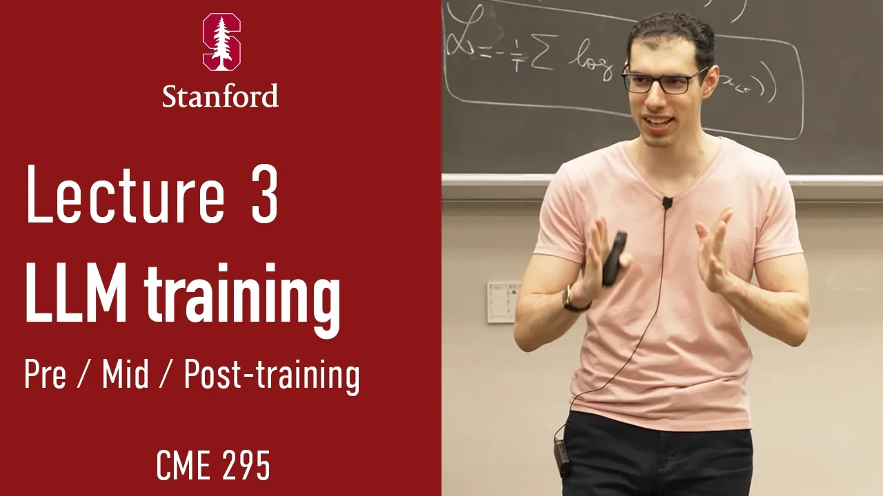
Stanford CME 295 Transformers & LLMs | Fall 2026 | Lecture 3 - LLM training — Stanford Online

Stanford Online

Transitioning foundational models from raw autoregressive pre-training to structured reasoning requires combining preference alignment, parameter-efficient adaptation, and reinforcement learning.

AI-assisted summary of Stanford CME 295 Transformers & LLMs | Fall 2026 | Lecture 3 - LLM training — original source. Check the original for full context.

Source published:

Key ideas

  • The foundation model paradigm replaces fragmented, task-specific architectures with unified pre-training followed by sequential adaptation stages, with modern frontiers scaling pre-training corpora up to 30 trillion tokens. (3:36)
  • Extending context windows during midtraining relies on modifying RoPE base frequencies via techniques like YaRN to prevent degradation caused by unseen position rotations, paired with best-fit document packing. (24:31)
  • Reasoning models replace sparse or uncalibrated human preference tuning with deterministic verification, utilizing algorithms like Group Relative Policy Optimization (GRPO) and On-Policy Distillation (OPD) to drive test-time chain-of-thought exploration. (79:07)
  • Multi-stage post-training RL pipelines risk catastrophic forgetting across reasoning and conversational domains, which frontier architectures mitigate through cross-stage on-policy distillation against prior checkpoints. (99:59)

Detailed notes

## Background Published on YouTube by Stanford Online on October 15, 2026, this video records Lecture 3 of the Stanford CME 295 course on Transformers and LLMs taught by Adjunct Professors Afshine Amidi and Shervine Amidi. The lecture provides an in-depth walkthrough of large language model training, spanning pretraining, cross-entropy loss, midtraining, supervised fine-tuning, parameter-efficient adaptations, preference alignment, and emergent reasoning methods.

## TL;DR The lecture provides a comprehensive technical overview of the end-to-end training pipeline for modern large language models. The instructors explain the foundations of autoregressive pretraining, cross-entropy loss derivation, and context extension techniques such as RoPE frequency interpolation during midtraining. They then unpack supervised fine-tuning and parameter-efficient methods like LoRA before dissecting preference tuning paradigms, including Bradley-Terry reward modeling, RLHF, and DPO. The session concludes with recent breakthroughs in reasoning elicitation, detailing verifiable rewards, Group Relative Policy Optimization (GRPO), on-policy distillation, and concrete architectural lessons from models like GLM-4 and GLM-5.

## Atmosphere & style The presentation maintains a polished, rigorously academic atmosphere that seamlessly integrates theoretical derivations with practical engineering intuition. Afshine and Shervine Amidi teach with a measured, accessible cadence, breaking down mathematical concepts from first principles while frequently challenging students to consider the physical computational trade-offs behind each technique. The delivery is lucid and candid, moving smoothly from chalkboard-style loss functions to nuanced discussions on industry topics such as model collapse, synthetic data distillation disputes, and open-weight transparency.

## Bulletin - [03:36](https://www.youtube.com/watch?v=S3bCDcJhz4s&t=216s) The foundation model paradigm replaces fragmented, task-specific architectures with unified pre-training followed by sequential adaptation stages, with modern frontiers scaling pre-training corpora up to 30 trillion tokens. - [24:31](https://www.youtube.com/watch?v=S3bCDcJhz4s&t=1471s) Extending context windows during midtraining relies on modifying RoPE base frequencies via techniques like YaRN to prevent degradation caused by unseen position rotations, paired with best-fit document packing. - [01:19:07](https://www.youtube.com/watch?v=S3bCDcJhz4s&t=4747s) Reasoning models replace sparse or uncalibrated human preference tuning with deterministic verification, utilizing algorithms like Group Relative Policy Optimization (GRPO) and On-Policy Distillation (OPD) to drive test-time chain-of-thought exploration. - [01:39:59](https://www.youtube.com/watch?v=S3bCDcJhz4s&t=5999s) Multi-stage post-training RL pipelines risk catastrophic forgetting across reasoning and conversational domains, which frontier architectures mitigate through cross-stage on-policy distillation against prior checkpoints.

## Key takeaways - [05:28](https://www.youtube.com/watch?v=S3bCDcJhz4s&t=328s) Pre-training relies on autoregressive next-token prediction and teacher forcing, which introduces an inherent exposure mismatch between ground-truth training inputs and purely model-generated inference sequences. - [10:33](https://www.youtube.com/watch?v=S3bCDcJhz4s&t=633s) Joint sequence probability decomposes via the chain rule, requiring negative log-likelihood transformation and sequence length normalization to avoid severe numerical underflow during optimization. - [14:01](https://www.youtube.com/watch?v=S3bCDcJhz4s&t=841s) Raw cross-entropy loss cannot be directly compared across different tokenizers; bits per byte (BPB) provides a standardized metric by normalizing loss using the token-to-byte ratio. - [16:21](https://www.youtube.com/watch?v=S3bCDcJhz4s&t=981s) In data-constrained regimes, training up to four epochs over high-quality data yields measurable performance gains rather than causing premature degradation. - [22:06](https://www.youtube.com/watch?v=S3bCDcJhz4s&t=1326s) Midtraining retains next-token prediction while shifting data distributions toward long-form code, technical literature, and frequency-adjusted positional embeddings to expand context capabilities. - [34:04](https://www.youtube.com/watch?v=S3bCDcJhz4s&t=2044s) Supervised fine-tuning (SFT) transforms base completion models into instruction-following assistants by computing cross-entropy loss solely over assistant response tokens while masking prompt tokens. - [40:51](https://www.youtube.com/watch?v=S3bCDcJhz4s&t=2451s) Low-Rank Adaptation (LoRA) freezes the base parameters and injects trainable low-rank rank-decomposition matrices, with modern practice prioritizing feed-forward network blocks where the bulk of compute and capacity reside. - [46:37](https://www.youtube.com/watch?v=S3bCDcJhz4s&t=2797s) Pairwise human preference comparisons are vastly more reliable than pointwise absolute scoring, forming the empirical foundation of the Bradley-Terry preference probability formulation. - [01:01:49](https://www.youtube.com/watch?v=S3bCDcJhz4s&t=3709s) Reinforcement Learning from Human Feedback (RLHF) optimizes a generative policy against a frozen reward model while penalizing KL divergence from an SFT reference checkpoint to prevent reward hacking. - [01:05:38](https://www.youtube.com/watch?v=S3bCDcJhz4s&t=3938s) Direct Preference Optimization (DPO) derives an analytical solution that optimizes preferences directly through the policy log-ratios relative to a reference model, bypassing an explicit reward model. - [01:19:07](https://www.youtube.com/watch?v=S3bCDcJhz4s&t=4747s) Verifiable reasoning domains such as mathematics and programming bypass human reward models entirely by leveraging unit tests and exact ground-truth outputs for deterministic evaluation. - [01:20:56](https://www.youtube.com/watch?v=S3bCDcJhz4s&t=4856s) Group Relative Policy Optimization (GRPO) computes advantages by comparing a sampled group of candidate completions against their internal baseline rather than relying on a separate critic network. - [01:23:31](https://www.youtube.com/watch?v=S3bCDcJhz4s&t=5011s) On-Policy Distillation (OPD) bridges sparse sequence-level reinforcement learning and dense token-level supervised learning by evaluating teacher signals over the student model's own on-policy generations. - [01:27:50](https://www.youtube.com/watch?v=S3bCDcJhz4s&t=5270s) Model collapse emerges when networks recursively train on finite or synthetic generations, systematically shedding rare long-tail distributions of human language and thought. - [01:39:59](https://www.youtube.com/watch?v=S3bCDcJhz4s&t=5999s) Frontier open-weight post-training frameworks divide reinforcement learning into specialized tracks—reasoning, agentic tool execution, and general alignment—to balance verifiable problem-solving with conversational nuance.

## Detailed walkthrough ### [00:05](https://www.youtube.com/watch?v=S3bCDcJhz4s&t=5s) Recap of Architectural Scaling, Chinchilla, and Efficient Attention

The lecture opens with enthusiasm as the instructors set out the agenda: moving beyond architecture to explore how to actually train large language models so that they align with end goals. Before diving into the training pipeline, the speaker reviews the key architectural concepts established in previous lectures. In Lecture 1, the foundational transformer was introduced, featuring both an encoder and a decoder. In Lecture 2, removing the encoder altogether yielded a simpler, decoder-only setup that reframed generative problems into a pure text-to-text formulation. Scaling these decoder-only models across parameter count and training token volume revealed consistent performance improvements described by empirical scaling laws.

However, compute budgets are finite. The speaker revisits a central takeaway from the Chinchilla paper: compute must be allocated optimally between model size and training data. Historically, many scaled-up architectures were severely undertrained because they failed to maintain the required ratio—roughly 20 tokens of training data for every single model parameter. The speaker also reviews methods introduced to keep large architectures computationally viable:

- **Mixture of Experts (MoE):** Rather than activating every parameter on every forward pass, MoE dynamically routes tokens to specific expert sub-networks located inside the feed-forward layers, where the vast majority of compute takes place. - **RoPE (Rotary Position Embeddings):** Replacing absolute position embeddings by injecting positional information directly within the attention mechanism itself. - **Attention Variants:** Moving away from standard global attention toward sliding-window attention to manage context length. - **Grouped-Query Attention (GQA):** Sharing key and value heads across multiple query heads to dramatically reduce the memory footprint of KV caches during sequence decoding. - **Modern Normalization:** Adopting updated normalization strategies to stabilize deep network activations.

[03:36](https://www.youtube.com/watch?v=S3bCDcJhz4s&t=216s) The Paradigm Shift: From Task-Specific Models to Pre-training

The discussion turns to the first stage of the modern LLM training pipeline: pre-training. To motivate why pre-training exists, the speaker contrasts modern practices with traditional machine learning paradigms from roughly fifteen years ago. Historically, practitioners trained narrow models strictly on a per-use-case basis—one bespoke model for spam detection, another for sentiment analysis, and yet another for machine translation. Each system learned language patterns entirely from scratch for its isolated task.

```mermaid flowchart TD accTitle: Paradigm Shift from Task-Specific Modeling to LLM Pre-training accDescr: Diagram contrasting traditional per-task training with the two-stage pre-training and task adaptation framework.

subgraph Traditional["Traditional ML (circa 15 years ago)"] direction TB T1["Spam Detection Data"] --> M1["Spam Classifier"] T2["Sentiment Data"] --> M2["Sentiment Classifier"] T3["Translation Pairs"] --> M3["Translation Model"] end

subgraph Modern["Modern Foundation Paradigm"] direction TB Data["Massive Web Data (Text, Code, Math)"] --> PT["Pre-trained Base LLM (Language Model)"] PT --> SFT["Task Specialization / Fine-Tuning"] SFT --> App1["Spam / Sentiment / Translation / General Chat"] end ```

The breakthrough of modern foundation models lies in transfer learning: conducting a single, massive, general-purpose pre-training stage to learn the fundamental structure of language, math, and code. Once acquired, that base knowledge is adapted or specialized for downstream objectives. The speaker notes: “Actually the idea behind what we want to do is to do a one-time big what we call pre-training to learn about language and then start from there if we want to specialize that for a specific use case.” Large language models have proven sufficiently general that they can often handle diverse tasks with minimal or no explicit re-training.

[05:28](https://www.youtube.com/watch?v=S3bCDcJhz4s&t=328s) Next-Token Prediction, Teacher Forcing, and Masked Self-Attention

During pre-training, the model is exposed to vast corpora assembled across the internet: English and multilingual web text, source code across languages like Python, mathematical derivations, and scientific articles. The learning objective across all this varied data is next-token prediction. An arbitrary tokenizer breaks raw text into tokens. Conceptually, the model receives a beginning-of-sequence token, predicts the first textual token, feeds that prediction forward to predict the second token, and repeats this iteratively across the whole document.

```mermaid flowchart LR accTitle: Next-Token Prediction with Masked Attention accDescr: Sequence flow showing input tokens passing through masked self-attention to generate next-token prediction probabilities under teacher forcing.

subgraph Inputs["Observed Sequence Context"] BOS["[BOS]"] --> X1["x₁"] X1 --> X2["x₂"] X2 --> Dots["..."] Dots --> Xprev["x_(t-1)"] end

subgraph Core["Model Forward Pass"] Xprev --> MaskedAttn["Masked Self-Attention (Decoders)"] MaskedAttn --> Probs["P_θ(x_t | x₁...x_(t-1))"] end

subgraph Objective["Supervision (Teacher Forcing)"] GroundTruth["True token: x_t"] -.->|"Cross-Entropy Loss"| Probs end ```

In practice, training does not proceed token by token sequentially. Because the ground-truth sequence is already known, the entire sequence is fed into the network simultaneously and computed as parallel matrix multiplications. This relies on teacher forcing: regardless of what probability distribution the network outputs at step $t$, the input presented to step $t+1$ is strictly the true historical token from the training document.

Two student questions prompt further clarification during the lecture: - **Exposure mismatch during inference:** A student points out that teacher forcing creates an inherent discrepancy between training and real-world generation, because during actual inference the model must consume its own potentially flawed outputs rather than clean ground truth. The instructor affirms the critique: “The question is: well, if you teacher force the model to learn a certain way, it is not actually having things it is generating itself as input. So there is a mismatch between training and inference. So that’s an excellent point and we will see actually how we can solve that later on.” - **Empty prompts at sequence starts:** Another student asks whether models are provided a prompt at the very beginning when only the beginning-of-sequence token is present. The instructor confirms that no prompt is used during base pre-training; receiving only the start token simply trains the model on the prior distribution of which tokens naturally open documents.

Crucially, parallel training over the full context without leaking future tokens is made possible by masked self-attention. The causal mask zeroes out attention weights for all positions after the current position, ensuring that the prediction for any position depends solely on earlier tokens and the token itself.

[10:33](https://www.youtube.com/watch?v=S3bCDcJhz4s&t=633s) First-Principles Derivation of the Cross-Entropy Loss

The speaker transitions from the intuitive framing of next-token prediction to a rigorous first-principles derivation of the standard LLM training objective. The overarching statistical goal is maximum likelihood estimation: finding a set of model parameters $\theta$ that maximizes the probability assigned by the model to the observed training sequences.

For an arbitrary sequence of $n$ tokens $X = (x_1, x_2, \dots, x_n)$, the joint probability under parameterization $\theta$ is:

$$P_\theta(X) = P_\theta(x_1, x_2, \dots, x_n)$$

Applying the chain rule of probability decomposes this joint probability into a product of autoregressive conditional probabilities:

$$P_\theta(x_1, \dots, x_n) = P_\theta(x_1) \cdot P_\theta(x_2 \mid x_1) \cdots P_\theta(x_n \mid x_1, \dots, x_{n-1}) = \prod_{t=1}^n P_\theta(x_t \mid x_1, \dots, x_{t-1})$$

The speaker emphasizes the numerical hazard of directly optimizing this product: “The problem with maximizing the product of probabilities which are each in between zero and one is that the product tends to zero. So it can lead to numerical instabilities.” Multiplying thousands of probabilities bounded between 0 and 1 causes severe underflow. To eliminate underflow and simplify optimization, standard practice applies the monotonic natural logarithm to convert the product into a summation:

$$\log P_\theta(X) = \sum_{t=1}^n \log P_\theta(x_t \mid x_1, \dots, x_{t-1})$$

Because standard deep learning optimization algorithms are formulated as minimization problems, the objective is inverted by taking the negative log-likelihood. Finally, to ensure the loss remains invariant to the length of the input sequence rather than scaling linearly with token count, the sum is normalized by the total number of tokens $n$, arriving at the canonical cross-entropy loss function:

$$\mathcal{L}(\theta) = -\frac{1}{n} \sum_{t=1}^n \log P_\theta(x_t \mid x_1, \dots, x_{t-1})$$

[14:01](https://www.youtube.com/watch?v=S3bCDcJhz4s&t=841s) Cross-Entropy Loss and Bits per Byte (BPB)

The predicted probability $P_\theta$ comes directly from the output of the model's final layer, where $\theta$ represents the network parameters, $x_t$ is the target token, $x_{<t}$ denotes the preceding context tokens, and $T$ is the total sequence length. Rather than memorizing the mathematical expression for cross-entropy loss, the speaker urges students to understand it intuitively from first principles: “So all that to say that you will find the cross entropy loss in a lot of places and just instead of memorizing this formula just think of it from first principles is just you trying to find parameters theta that maximize the probability of your model seeing the training data.”

However, a subtle complication arises when evaluating or comparing models: cross-entropy loss values are fundamentally tied to the choice of tokenizer. Because different tokenizers segment identical text into varying numbers of tokens, the raw loss values across models with distinct vocabularies are not directly comparable. To achieve a tokenizer-independent metric, practitioners rescale the loss into bits per byte (BPB). This normalization multiplies the standard cross-entropy loss by the ratio of tokens to bytes ($T / B$, where $B$ is the total byte count of the input text) and scales it by $\frac{1}{\log(2)}$ to convert the units into information-theoretic bits. Addressing an audience question regarding the variable $B$, the speaker clarifies that $B$ simply counts the raw bytes in the input text, reflecting the byte-level representation of characters.

```mermaid flowchart LR accTitle: Cross-Entropy Loss to Bits per Byte Conversion accDescr: Diagram showing how standard cross-entropy loss is scaled by sequence lengths and log base 2 to produce tokenizer-independent bits per byte. A["Raw Cross-Entropy Loss"] --> B["Scale by (Tokens / Bytes)"] B --> C["Scale by 1 / log(2)"] C --> D["Bits per Byte (BPB)"] ```

- $P_\theta$: Probability distribution over vocabulary predicted by the final model layer. - $x_t$: Target token at index $t$. - $x_{<t}$: History of preceding tokens up to time $t-1$. - $T$: Total number of tokens in the sequence. - $B$: Total number of raw input bytes. - BPB Formula scaling factor: $\frac{T}{B} \times \frac{1}{\log(2)}$.

---

[16:21](https://www.youtube.com/watch?v=S3bCDcJhz4s&t=981s) Decoder-Only Masking and Pretraining Data Regimes

A student asks whether masked self-attention—used to prevent tokens from attending to subsequent future positions—applies only to decoders or if it is also relevant for encoders. The speaker clarifies that standard auto-regressive pretraining operates strictly in a decoder-only regime: “So here in this case we don't have an encoder and we only have a decoder and our goal is to predict the next token. We need to make sure that when we predict the next token, we can only rely on the things that we have decoded so far to mimic the inference setup.” Encoder-only architectures cannot perform step-by-step auto-regressive generation unless altered significantly, a topic reserved for lecture 8.

The discussion then moves to pretraining corpora. Building modern LLMs requires vast corpora comprising trillions—and increasingly tens of trillions—of tokens drawn from the open web, code repositories, mathematics, and scientific literature. Addressing a previous lecture's question about whether data can ever be repeated during pretraining, the speaker points to empirical studies examining data-constrained regimes. When fresh tokens are limited, models benefit from multiple training epochs over identical data rather than stopping early: “The question is would you rather stop the training or is it worth for you actually training multiple times on the same tokens and the answer in this case is actually yes up to four times.” Repeating high-quality data up to four epochs yields clear performance gains without degrading general capabilities.

---

[19:16](https://www.youtube.com/watch?v=S3bCDcJhz4s&t=1156s) Data Mixture Strategies and Pretraining Scale

Careful data mixture design has become as critical as model architecture. To disentangle whether benchmark gains stem from architectural tweaks or cleaner data, benchmarks like DataComp-LM standardize model parameters so researchers can isolate the exact contribution of data quality. When determining the precise recipe—such as the proportion of code versus general web text—practitioners often run proxy experiments by training small auxiliary models on diverse candidate mixtures and extrapolating the optimal ratio for large-scale training.

```mermaid flowchart TD accTitle: Pretraining Data Mixture and Scaling Pipeline accDescr: Pipeline showing data curation, small model mixture searches, and massive scale pretraining. subgraph Sourcing ["Data Sourcing & Cleaning"] W["Web Text"] C["Code Repositories"] M["Math & Science"] end subgraph Selection ["Mixture Optimization"] Proxy["Train Small Proxy Models"] Search["Evaluate Data Mixtures (e.g., DataComp-LM)"] end subgraph Pretraining ["Scale Pretraining"] Scale["Train Base Model (Trillions of Tokens)"] end Sourcing --> Selection Proxy --> Search Search --> Scale ```

The data curation pipelines powering top open-weight models are massive engineering endeavors. Citing OLMo 2 (or OLMo-style open pipelines) and GLM-4/GLM-5 as examples, the speaker notes that pretraining now reaches mind-boggling magnitudes: - GLM-4/GLM-5 was trained on 30 trillion tokens as a modern point of reference. - Designing data mixes frequently involves searching over combinations (e.g., 20% code, 50% web text) evaluated via small models before scaling. - The underlying infrastructure and distributed computing required to train across tens of trillions of tokens will be explored in depth during Lecture 5.

---

[22:06](https://www.youtube.com/watch?v=S3bCDcJhz4s&t=1326s) Midtraining: Domain Injection and Long Context Adaptation

While traditional LLM development proceeded directly from pretraining to alignment, modern recipes insert an intermediate phase termed *midtraining*. This phase retains next-token prediction objectives but shifts data distribution to achieve two distinct goals: domain knowledge injection and sequence length extension. Domain injection feeds the model specialized, curated datasets rich in code, reasoning chains, and mathematical proofs.

The second core driver of midtraining is long-context training. Standard pretraining runs on relatively short sequence lengths—often around 4,000 tokens—for computational efficiency. However, downstream deployment demands contexts reaching 128k, 200k, or more tokens. Because Rotary Position Embeddings (RoPE) rely on rotational angles calculated relative to sequence indices, directly exposing a model to long contexts at inference without preparation causes substantial degradation: “the reality is that your model actually has never seen the rotations of these longer sequences. So it may get confused.”

- Midtraining retains standard next-token prediction loss. - Injects specialized domains (e.g., advanced coding, scientific literature, formal proofs). - Expands typical base pretraining lengths (e.g., 4k tokens) up to 128k–200k tokens.

---

[24:31](https://www.youtube.com/watch?v=S3bCDcJhz4s&t=1471s) RoPE Frequency Scaling, Interpolation, and YaRN

To bridge the gap between short pretraining windows and massive target contexts, engineers adapt Rotary Position Embeddings rather than introducing newly learned positional weights. Naive extrapolation forces the network to process unseen, high-magnitude rotational position differences. Instead, methods such as YaRN apply frequency interpolation, effectively compressing long sequence distances back into the familiar rotational range observed during short-context pretraining.

Responding to student questions about how target context windows are determined and executed, the instructor explains that target context sizes are planned in advance. Models adopt curriculum learning: pretraining initiates on short windows (e.g., 4k tokens), midtraining extends sequences to predetermined targets (such as 128k or 200k tokens) using modified RoPE frequencies, and those modified frequencies carry through downstream inference: “So they would initially train the model for short context on some frequencies and then they perform mid training, they perform long context training in which they tweak a little bit the frequencies and then they use these frequencies for inference and so on.” Answering a follow-up on whether methods like YaRN replace the RoPE architecture entirely, the speaker clarifies that the core RoPE structure remains intact; only the underlying base frequencies are rescaled to match the domain of familiar rotations.

[27:38](https://www.youtube.com/watch?v=S3bCDcJhz4s&t=1658s) Challenges of Long-Context Training and Knowledge Cutoffs

Scaling context length from a baseline of 4,000 tokens up to hundreds of thousands of tokens introduces substantial computational and data engineering hurdles. Because standard Transformer architectures rely on self-attention, where every token attends to every other token, computational complexity scales quadratically ($O(n^2)$) with sequence length. Beyond compute, generating and curating high-quality training data that demands true long-range reasoning is exceedingly difficult. The training objective requires the model to learn to leverage information positioned far back in the context window to predict a token deep in the sequence. Sourcing or synthesizing naturally occurring observations where a correct token prediction strictly depends on distant past context requires non-trivial data curation.

Once a foundation model completes pretraining, mid-training, and long-context adaptation—at the expense of significant capital—it emerges with extensive general world knowledge, natural language understanding, and coding capabilities. However, that knowledge remains static, permanently bounded by a fixed knowledge cutoff date. If a user queries the model regarding events occurring after that cutoff, the base model cannot answer natively because that information was absent during training.

```mermaid flowchart LR accTitle: Base Pretraining Stages and Cutoff accDescr: Progression from pretraining through mid-training to long-context training, resulting in a static knowledge base.

subgraph Pipeline["Pretraining Pipeline"] PT["General Pretraining"] --> MT["Domain Mid-Training"] MT --> LC["Long-Context Scaling"] end

LC --> Base["Base Foundation Model"] Base --> KO["Fixed Knowledge Cutoff Date"] ```

- **Computational Scaling**: Self-attention incurs an $O(n^2)$ computational overhead, making scaling from 4,000 to hundreds of thousands of tokens computationally expensive. - **Data Dependency Bottleneck**: Models must be provided observations specifically designed so that future token predictions necessitate resolving dependencies situated far in the preceding context. - **Knowledge Cutoff Example**: As an illustrative hypothetical, a model like “GPT-6 Astra” trained up to April 30, 2026, possesses zero internal awareness of real-world events occurring after that date.

---

[30:39](https://www.youtube.com/watch?v=S3bCDcJhz4s&t=1839s) The Autocomplete Failure and the Need for Supervised Fine-Tuning (SFT)

A base model fresh out of pretraining, mid-training, and long-context training operates purely via autoregressive next-token prediction. It has not been conditioned to act as a conversational assistant. To illustrate this limitation, the lecturer presents a hypothetical prompt to the class: *“Can I put my teddy bear in the washer?”* Instead of answering the user's practical query, a raw base model merely autocompletes text in the style of internet prose: *“Teddy bears are often made of materials like polyester and cotton with plastic eyes and sometimes small accessories.”*

The lecturer emphasizes the fundamental limitation of base models for interactive applications:

> “Is it useful? No, it's not useful. So, we're not done. This was pre-training. Now, let's go into the next stage, which is trying to make our LLM useful.”

To convert a next-token text autocompletion engine into a practical assistant, practitioners turn to Supervised Fine-Tuning (SFT). SFT alters the model's behavioral alignment by exposing it to curated input-output pairs $(x, y)$, where $x$ represents an instruction or prompt and $y$ denotes the target response. Although the optimization objective remains standard cross-entropy over tokens, the structural formulation differs: the model is conditioned on the full prompt $x$, but the loss function strictly penalizes errors on the generated response tokens $y$.

```mermaid flowchart TD accTitle: SFT Loss Masking Flow accDescr: Conditioning on prompt input x without loss calculation, calculating cross-entropy loss solely over response tokens y.

subgraph Inputs["Input Sequence"] X["Instruction Prompt (x)"] Y["Target Response (y)"] end

subgraph ForwardPass["Transformer Forward Pass"] X -->|"Prompt Masked (Zero Loss)"| LLM["LLM"] Y -->|"Autoregressive Prediction"| LLM end

LLM --> CE["Cross-Entropy Loss on y_t given (x, y_<t)"] ```

---

[34:04](https://www.youtube.com/watch?v=S3bCDcJhz4s&t=2044s) SFT Mechanics, Loss Masking, and Data Regimes

Addressing a student question regarding how SFT differs conceptually from mid-training, the lecturer clarifies that mid-training involves continuing next-token prediction over raw corpora of higher-quality or specialized domain text (such as mathematics or code) without an explicit instruction-following format. SFT, by contrast, explicitly conditions the network on an input prompt $x$ and models the conditional probability of target response tokens $y = (y_1, y_2, \dots, y_T)$:

$$\mathcal{L}_{\text{SFT}}(\theta) = - \sum_{t=1}^{T} \log P_\theta(y_t \mid x, y_{<t})$$

In response to another student asking whether predicting the input prompt is penalized during backpropagation, the lecturer confirms that the loss across prompt tokens $x$ is masked out completely:

> “The question is, do you penalize predicting the input? The answer is no. You only penalize predicting the output. You don't care about the input. The input is given to you.”

The dataset volume required for SFT is substantially smaller than pretraining: - **Domain-Specific SFT**: Narrow specialized tasks (such as generating poetry in a distinct meter or style) can be achieved with hundreds to thousands of targeted examples. - **General Assistant Tuning**: Broad instruction-following capabilities spanning varied domains typically require on the order of millions of high-quality paired examples—orders of magnitude less data than the trillions of tokens digested during pretraining.

When evaluated on the earlier prompt (*“Can I put my teddy bear in the washer?”*), an instruction-tuned SFT model provides an actionable answer: *“No, it might get damaged. Try hand washing instead.”*

---

[38:42](https://www.youtube.com/watch?v=S3bCDcJhz4s&t=2322s) SFT Challenges and the Motivation for LoRA

While SFT aligns base models into direct assistants, it introduces critical training challenges: 1. **Data Quality and Behavioral Mimicry**: Because models mirror the stylistic and behavioral nuances of their SFT datasets, low-quality demonstrations degrade outputs immediately. 2. **Distributional Bias**: Skewed prompt mixtures cause the network to overfit specific phrasing, tones, or response lengths, harming zero-shot generalization on unseen formats. 3. **Compute and Memory Constraints**: Modern LLMs span tens to hundreds of billions of parameters. Updating all model weights across full parameter matrices during fine-tuning demands vast GPU memory for optimizer states, gradients, and checkpoints.

Because the underlying model already possesses rich syntactic, semantic, and factual knowledge from pretraining, modifying every single weight matrix to steer conversational behavior is fundamentally redundant:

> “The idea behind LoRa is you actually probably don't need to update all the weights of your model in order to behave a certain way because you're you're almost there already.”

This insight motivates parameter-efficient fine-tuning (PEFT) methods, leading directly into Low-Rank Adaptation (LoRA), which freezes the original model parameters and injects low-rank trainable weight matrices into the network architecture.

[40:51](https://www.youtube.com/watch?v=S3bCDcJhz4s&t=2451s) Low-Rank Adaptation (LoRA) Mechanics and Efficiency

The discussion continues on Low-Rank Adaptation (LoRA) and how it alters model updates. Instead of updating the full weight tensor, the weight matrix is decomposed into the pre-trained, already learned weights $W_0$ plus tunable parameters. These tunable parameters live in much lower-rank matrices—denoted as $B$ and $A$—which dramatically cuts the parameter count required during fine-tuning. This parameter reduction makes training vastly more computationally efficient while achieving roughly on-par performance with full fine-tuning, depending on dataset size and task complexity.

Beyond compute savings during training, LoRA provides massive storage advantages when serving multiple tasks. In a production environment with several distinct use cases—such as spam detection, sentiment analysis, or translation—an engineer does not need to duplicate and store the full set of model weights for every single downstream application. Instead, the pre-trained base model $W_0$ is stored once, and each task only requires saving its unique low-rank adapters ($B$ and $A$). As the instructor summarizes: “So in other words, if you didn’t use LoRA, you would have to store all the weights for the first one, all the weights for the second one, and so on. But here you only need to store the delta.”

The architectural targets for LoRA have also evolved since the method was introduced: - **Original recommendation:** The original LoRA authors proposed injecting the low-rank adaptation matrices solely into the self-attention layers of the Transformer. - **Current best practice:** Subsequent empirical studies and experiments across diverse datasets demonstrate that adapting the feed-forward neural network (FFN / MLP) blocks yields substantial performance gains. Because the feed-forward layers contain a majority of the model’s parameters and account for most of the raw compute, adapting them provides higher expressive capacity. - **Recommended reading:** A notable write-up (referenced from Thinking Machines / similar technical publications) is highlighted in the course slides for students seeking a deeper dive into optimal LoRA parameter placement.

```mermaid flowchart LR accTitle: LoRA Weight Decomposition Flow accDescr: Diagram showing how a pre-trained base model combines with task-specific low-rank delta matrices to produce adapted outputs. subgraph Base["Frozen Shared Base"] W0["Base Weights W0<br/>(Frozen)"] end subgraph Adapters["Task-Specific Low-Rank Adapters"] direction TB Spam["Spam Task:<br/>B_spam * A_spam"] Sent["Sentiment Task:<br/>B_sent * A_sent"] Trans["Translation Task:<br/>B_trans * A_trans"] end W0 --> Spam W0 --> Sent W0 --> Trans ```

---

[43:40](https://www.youtube.com/watch?v=S3bCDcJhz4s&t=2620s) Student Q&A: Serving Adapters vs. Full Fine-Tuning

A student asks how an incoming prompt is routed to the correct weights when multiple LoRA adapters exist. The instructor clarifies that for a general-purpose conversational assistant, teams do not typically deploy fragmented task-specific checkpoints; instead, they train a single unified model that absorbs as much breadth and instruction-following capability as possible. Multiple adapter matrices are reserved for bespoke, highly specialized applications where a general model cannot suffice.

Another student questions why one would bother with parameter-efficient techniques like LoRA during Supervised Fine-Tuning (SFT) given that SFT datasets are around $10^6$ examples—orders of magnitude smaller than pre-training corpora. The instructor provides two practical justifications. First, hardware limitations prevent most practitioners and independent researchers from updating hundreds of billions of parameters: “Well, people who want to fine-tune, they usually people like you and I, we don’t have super big hardware and so we cannot afford having to tune billions and hundreds of billions of parameters.” Second, the foundational base model already contains the world knowledge; re-tuning every parameter introduces unnecessary degrees of freedom when the target behavior only requires small steering adjustments.

The Q&A wraps up with two points on industry divergence and parameter update cadence: - **Model differentiation across companies:** Whether models diverge at this stage depends on underlying architectural choices and proprietary data mixtures, with the exact dataset composition being the decisive differentiator. - **Update cadence:** Weight updates depend heavily on business constraints. When long, complex system prompts become too expensive or token-heavy for production APIs, fine-tuning the weights once to permanently bake in the desired behavior saves considerable inference cost over time.

---

[46:37](https://www.youtube.com/watch?v=S3bCDcJhz4s&t=2797s) The Need for Preference Tuning and Negative Guidance

Up to this point, LLM training focused on acquiring knowledge via pre-training and learning to follow task templates via SFT. However, SFT alone only demonstrates what the model *should* do, leaving a critical gap in teaching it what *not* to do. The instructor illustrates this shortfall with a failure mode:

> Prompt: *“Suggest a new activity I could do with my teddy bear.”* > LLM output: *“Well, I suggest you actually do not spend time with the teddy bear.”*

While technically a syntactically valid completion, this unhelpful or dismissive output is not what users want. SFT trains the model via next-token prediction on curated demonstrations without accounting for the fact that the training tokens were externally forced onto the model rather than generated from its own probability distribution. To prevent undesirable behaviors, systems require preference alignment. When a model consistently misbehaves, it often reveals artifacts or low-quality demonstrations unintentionally included in the SFT training mixture.

Human feedback can theoretically be formatted in three scoring paradigms: 1. **Pointwise scoring:** Assigning an absolute quality score to an individual response in isolation. This approach is notoriously unreliable because human evaluators struggle to maintain calibrated absolute judgment scales across disparate prompts. 2. **Listwise ranking:** Presenting a prompt alongside a ranked list of candidate responses ordered from most preferred to least preferred. 3. **Pairwise comparisons:** Presenting a single prompt alongside two candidate responses (one positive/chosen, one negative/rejected). Pairwise comparison is the industry standard because relative human judgment is vastly more consistent: “So as a human it is much simpler for you to figure out that something is better than something else as opposed to stating that something is good in absolute scale.”

---

[51:37](https://www.youtube.com/watch?v=S3bCDcJhz4s&t=3097s) Reward Modeling and Reinforcement Learning from Human Feedback (RLHF)

To align language models using preference data at scale, practitioners cannot rely on humans to grade every new output the model might generate. The solution is a two-stage alignment framework powered by **Reward Modeling** and **Reinforcement Learning from Human Feedback (RLHF)**:

1. **Reward Modeling:** Train a separate model (the reward model) on collected pairwise human preference comparisons so it learns to score any arbitrary prompt-response pair, assigning higher scalar rewards to helpful, benign responses and lower rewards to poor or harmful ones. 2. **Policy Optimization (RLHF):** Optimize the generative language model against the learned reward model using reinforcement learning, maximizing generated outputs that earn high reward scores while penalizing generations that receive low scores.

The instructor highlights why the technique earned its name: “Because in the first stage where you want to learn how to distinguish good from bad, you are training your reward model on human preference data.”

Reinforcement learning formulations introduce significant mathematical machinery compared to standard supervised learning. The lecture concludes by framing this overview as an intuitive conceptual primer, setting expectations that the rigorous mathematical derivation—including policy gradients and optimization objectives—will be unpacked in depth during the following lecture.

[54:04](https://www.youtube.com/watch?v=S3bCDcJhz4s&t=3244s) Reward Modeling and the Bradley-Terry Formulation

Preference tuning proceeds in two core stages: reward modeling followed by reinforcement learning. In the reward modeling phase, the objective is to teach a model how to distinguish between good and bad responses given a specific prompt. For any input prompt paired with candidate answers, the reward model must output a scalar judgment indicating whether the response is desirable.

To mathematically express the preference between responses, practitioners standardly adopt the Bradley-Terry model. This formulation states that the probability of a candidate response $y_i$ being preferred over another response $y_j$ is given by the sigmoid ($\sigma$) of the difference between their respective scalar rewards, $r_i$ and $r_j$:

$$P(y_i \succ y_j) = \sigma(r_i - r_j)$$

The sigmoid function, defined as $\sigma(x) = \frac{1}{1 + e^{-x}}$, smoothly maps any real-valued difference to a valid probability in the range $(0, 1)$, tending toward $0$ as $x \to -\infty$ and $1$ as $x \to +\infty$.

Training this reward model relies directly on collected pairwise preference data, which is the most practical format to gather from evaluators. Each data point consists of an input prompt $x$, a winning response $y_w$, and a losing response $y_l$. The reward model is trained via a pairwise loss function. Parallel to cross-entropy training—where model parameters $\theta$ are chosen to maximize the likelihood of observed training data—reward model training maximizes the probability that the model assigns a higher preference to the winning response over the losing response:

$$\max_\theta P(y_w \succ y_l \mid x) = \max_\theta \sigma\big(r_\theta(x, y_w) - r_\theta(x, y_l)\big)$$

Because probabilities can become vanishingly small and lead to numerical instability, and because machine learning workflows standardly minimize loss rather than maximize likelihood, the objective is converted by taking the negative logarithm. The final pairwise loss minimizes:

$$\mathcal{L}_\text{RM}(\theta) = -\mathbb{E}_{(x, y_w, y_l)}\left[\log \sigma\big(r_\theta(x, y_w) - r_\theta(x, y_l)\big)\right]$$

When a student inquires about the symbol $\mathbb{E}$, the instructor confirms that it simply represents the expectation over the dataset, functioning intuitively as a sum or average across all pairwise examples.

```mermaid flowchart LR accTitle: Reward Model Scoring and Bradley-Terry Formulation accDescr: Diagram showing how a prompt and two candidate responses are scored by a reward model and evaluated through a sigmoid difference. subgraph INPUTS["Input Data"] P["Prompt (x)"] YW["Winning Response (yw)"] YL["Losing Response (yl)"] end subgraph RM["Reward Model r_theta"] RW["Scalar Reward: r(x, yw)"] RL["Scalar Reward: r(x, yl)"] end DIFF["Difference: r(x, yw) - r(x, yl)"] SIG["Sigmoid: P(yw > yl)"]

P & YW --> RW P & YL --> RL RW & RL --> DIFF DIFF --> SIG ```

- **Reward model architectures**: - *LLM backbone with a classification head*: Takes the base autoregressive language model, extracts the final token's embedding representation, and projects it into a scalar reward value. This allows full reuse of the pretrained model weights. - *Encoder-only model*: Feeds the full prompt-response pair through bidirectional self-attention and projects the output directly to a scalar score. - **Supervision source**: Human preference comparisons provide the underlying ground-truth labels required for Reinforcement Learning from Human Feedback (RLHF).

---

[01:01:49](https://www.youtube.com/watch?v=S3bCDcJhz4s&t=3709s) Reinforcement Learning from Human Feedback (RLHF)

Once the reward model has learned to evaluate response quality, training transitions to the reinforcement learning phase. The instructor notes that this is the “more mathematically involved stage,” where the goal shifts to modifying the weights of the primary language model so its generated text maximizes the scores predicted by the reward model.

In this workflow, the prompt is fed into the generative LLM, which outputs a response. That generated pair is routed to the reward model, which evaluates whether the behavior should be encouraged or discouraged. The resulting scalar reward signal is used to compute gradient updates for the LLM. The instructor emphasizes a critical architectural distinction: during this stage, the reward model trained in step one is completely frozen; only the generative LLM's weights are being updated.

The RL objective function balances two competing forces: 1. **Reward maximization**: Encouraging the policy to produce sequences that achieve higher reward model scores. 2. **KL divergence / reference penalty**: Constraining the updated policy from straying too far from the reference model (typically the supervised fine-tuned, or SFT, checkpoint).

Preventing excessive divergence is critical because the reward model is an imperfect surrogate. Without a reference anchor, models fall prey to "reward hacking"—a failure mode where the policy exploits flaws and blind spots in the reward model to generate outputs that achieve high scores despite being unnatural, incoherent, or unhelpful to human evaluators.

When asked specifically how policy gradients and weight updates are computed under the hood, the instructor defers the detailed derivations: “save your question for next week. We'll go into that in detail. But the one thing I want you to remember here is in this stage the reward model is fixed. We're not updating its weights. We're only updating the the weights of the LLM.”

- **Data scale**: RL training typically operates across prompt sets that are orders of magnitude larger than the preference datasets used to train the reward model. - **Initialization**: The policy model begins directly from the weights of the supervised fine-tuning (SFT) stage.

---

[01:05:38](https://www.youtube.com/watch?v=S3bCDcJhz4s&t=3938s) Direct Preference Optimization (DPO)

While RLHF offers a powerful alignment mechanism, it is notoriously cumbersome in practice: it demands maintaining multiple models simultaneously (the active policy, the reference model, and the reward model), tuning sensitive reinforcement learning hyperparameters, and navigating optimization instabilities. As an alternative, Direct Preference Optimization (DPO) reframes preference alignment into a stable, supervised objective.

The instructor highlights that DPO eliminates the need for an explicit, standalone reward model entirely. By analytically expressing the optimal reward function in terms of the ratio between the policy model $\pi_\theta(y \mid x)$ and the frozen reference model $\pi_\text{ref}(y \mid x)$, DPO derives a closed-form loss that directly updates the LLM:

$$r(x, y) \propto \beta \log \frac{\pi_\theta(y \mid x)}{\pi_\text{ref}(y \mid x)}$$

When substituted into the Bradley-Terry formulation, the resulting loss structurally mirrors the reward model loss from earlier, but operates entirely over sequence probabilities:

$$\mathcal{L}_\text{DPO}(\theta) = -\mathbb{E}_{(x, y_w, y_l)}\left[\log \sigma\left(\beta \log \frac{\pi_\theta(y_w \mid x)}{\pi_\text{ref}(y_w \mid x)} - \beta \log \frac{\pi_\theta(y_l \mid x)}{\pi_\text{ref}(y_l \mid x)}\right)\right]$$

Intuitively, this loss mechanism simultaneously pulls two optimization levers: - It actively increases the probability of generating the winning response $y_w$ relative to the reference policy. - It actively decreases the probability of generating the losing response $y_l$ relative to the reference policy.

By bypassing reinforcement learning loops and freezing a copy of the reference model, DPO provides preference alignment through standard supervised classification mechanics.

[01:07:24](https://www.youtube.com/watch?v=S3bCDcJhz4s&t=4044s) The DPO Loss Function and Bradley-Terry Formulation

The Direct Preference Optimization (DPO) objective optimizes a loss function constructed to maximize the difference between the implicit reward of the winning response and that of the losing response ($R_w - R_l$). The mathematical formulation frames this as minimizing the negative expectation of the logarithm of the sigmoid applied to the reward difference:

$$\mathcal{L}_{\text{DPO}} = - \mathbb{E} \left[ \log \sigma (R_w - R_l) \right]$$

Here, the implicit reward $R$ is expressed in terms of a scaling factor multiplied by the log-ratio of the probability assigned by the model being trained ($\pi$) to the probability assigned by a frozen reference model ($\pi_{\text{ref}}$):

$$R(x, y) \propto \log \left( \frac{\pi(y \mid x)}{\pi_{\text{ref}}(y \mid x)} \right)$$

To drive the difference $R_w - R_l$ as large as possible, the optimization increases the probability of the winning output $y_w$ under the trained model relative to the reference model, while decreasing the probability of the losing output $y_l$. Answering a student's question about the notation $\pi$, the instructor explains that in reinforcement learning terminology, the language model is treated as a policy ($\pi$). Responding to a follow-up query about $\pi_{\text{ref}}$, the instructor confirms: “Yes, it is the model that you start from when you perform that training.” Reassuring the class about the mathematical complexity, the instructor remarks: “I just want to say that this formula can be scary but if you take the Bradley Terry formulation in minds and interprets the left and right term as a function of the ratio between what the model that you're trying to tweak over the reference model. If you think about that this way, then hopefully it makes a bit more sense.”

```mermaid flowchart TD accTitle: Direct Preference Optimization Probability Adjustment accDescr: Diagram showing how DPO increases winning token probabilities and decreases losing token probabilities relative to a reference model. subgraph Loss["DPO Loss: Maximize (Rw - Rl)"] direction TB RW["Winning Reward Rw = log( π(yw|x) / π_ref(yw|x))"] RL["Losing Reward Rl = log( π(yl|x) / π_ref(yl|x))"] end subgraph Update["Model Policy Adjustments"] UpWin["Increase π(yw | x)"] DownLose["Decrease π(yl | x)"] end RW --> UpWin RL --> DownLose ```

---

[01:10:15](https://www.youtube.com/watch?v=S3bCDcJhz4s&t=4215s) Comparing RLHF and DPO

Comparing Reinforcement Learning from Human Feedback (RLHF) to DPO highlights key differences in training setup and data dynamics. RLHF requires two distinct stages: first, training a separate reward model on preference pairs; second, optimizing the language model policy using reinforcement learning algorithms. Consequently, RLHF requires maintaining and updating multiple models, making it computationally heavy. In contrast, DPO reformulates the problem into an elegant, closed-form supervised learning objective that bypasses explicit reward modeling altogether.

However, an important architectural distinction lies in whether the optimization is *on-policy* or *off-policy*. DPO evaluates the loss on static, pre-collected completion pairs rather than completions freshly generated by the active model checkpoint during training. The instructor emphasizes: “RLHF is an on policy method because it is actually leveraging the actual outputs from the LLM which contrasts with off policy methods which are actually training the model based on fixed outputs that are not necessarily generated by the model.”

Returning to the running example—a user asking, *"Can I put my teddy bear in the washer?"*—the instructor contrasts an instruction-finetuned output with a preference-tuned output. Instead of a blunt *"No,"* a preference-aligned model produces a gentler, more conversational response: *"No, it's better not to; your teddy could get hurt. A gentle hand wash is safer."*

| Feature | Reinforcement Learning from Human Feedback (RLHF) | Direct Preference Optimization (DPO) | |:--- |:--- |:--- | | **Stages** | 2 stages (Reward modeling + Reinforcement learning) | 1 stage (Direct supervised optimization) | | **Model Footprint** | Multi-model (Policy, Reference, Reward, Critic) | Dual-model (Trained policy + Reference model) | | **Compute Overhead** | High / Compute-heavy | Lower / Supervised finetuning overhead | | **Policy Nature** | On-policy (generates fresh outputs during RL) | Off-policy (evaluates fixed, pre-existing outputs) |

---

[01:12:08](https://www.youtube.com/watch?v=S3bCDcJhz4s&t=4328s) The Shift Toward Reasoning Models

The lecture transitions to reasoning, defined simply as “the ability to solve a problem.” The instructor contrasts pure knowledge-retrieval prompts with reasoning-intensive prompts. Asking *“What is the course code for Stanford's transformers and LLMs class?”* is a factual lookup: “it's something that you know you know you don't know.” By contrast, asking *“Your bear was born in 2020. How old is the bear now?”* requires deduction: identifying the current year, computing the arithmetic difference, and arriving at the correct final number.

Earlier techniques relied on Chain-of-Thought (CoT) prompting, where few-shot demonstrations explicitly nudged the model to articulate its reasoning path step by step before generating the answer. However, the instructor notes: “The problem with that method is we don't want to always tell the LM to do that we want the LM to do that by itself and this is exactly what we will see here.”

Tracing the historical development: - **September 2024:** OpenAI becomes the first company to demonstrate marked jumps on mathematics and code benchmarks using automated internal reasoning mechanisms. - **Late 2024 / Early 2025:** Other frontier AI labs adopt similar reasoning strategies across their flagship architectures. - **January 2025:** DeepSeek-R1 is released as the first open-weights model to publicly document the exact training methodology behind reasoning models.

---

[01:15:09](https://www.youtube.com/watch?v=S3bCDcJhz4s&t=4509s) Reasoning Chains: UI Evolution, Privacy, and Pricing

The user interface design of reasoning models has evolved significantly. In early 2025, applications explicitly highlighted model thinking—such as OpenAI's interfaces displaying a *“thinking”* label, a timer showing how many seconds the model deliberated, an expandable reasoning summary, and a manual option to *“think more.”* Over time, reasoning models became standard across all product tiers, and consumer interfaces reduced these indicators to a simple thinking effort parameter.

Hiding intermediate reasoning chains from end users is driven by two major concerns: 1. **Privacy and Safety:** As demonstrated in published research, querying certain third-party provider APIs allows attackers to reconstruct the underlying reasoning chains. These traces often ingest and reflect sensitive user context, previous chat history, and system instructions that providers cannot safely expose. 2. **Competitive Distillation:** Exposing complete reasoning traces allows competitor labs to collect those chains and use them directly as high-grade training datasets to distill equivalent capabilities into rival models.

The instructor also cautions students regarding inference costs: intermediate reasoning tokens count as generated output tokens. When utilizing reasoning models through an API, users are billed for both the visible response and the hidden reasoning tokens produced during the generation step. When asked if models choose when to reason, the instructor confirms that models are trained to allocate internal reasoning effort adaptively based on prompt difficulty, though users can also modulate this via UI toggles.

```mermaid flowchart LR accTitle: User Input to Reasoned Output Flow accDescr: Workflow showing user prompt ingestion, internal thinking token generation, billing capture, and the final response. Input["User Prompt"] --> Delib["Internal Reasoning Chain<br/>('Thinking Tokens')"] Delib --> Billed["Token Accounting<br/>(Charged as Output Tokens)"] Delib --> Response["Final Visible Answer"] Billed -.-> Hidden["Hidden from UI / Protected"] Delib -.-> Hidden ```

---

[01:19:07](https://www.youtube.com/watch?v=S3bCDcJhz4s&t=4747s) Training with Verifiable Rewards

Training a model to self-generate reasoning chains relies on reinforcement learning with verifiable reward signals, differing fundamentally from subjective preference scoring. For domains such as mathematics and software engineering, solutions possess unambiguous, objective truth criteria: - **Coding benchmarks:** Code completions can be piped directly into sandbox environments and verified against predefined unit tests and edge cases. - **Mathematical tasks:** Symbolic derivations or numerical conclusions can be parsed and matched deterministically against exact ground-truth answers.

Because every generated response can be evaluated as strictly correct or incorrect without relying on human evaluators or noisy reward models, training environments can construct deterministic, rule-based reward functions based directly on the final output.

- Non-verifiable tasks require human raters or learned reward models to assess subjective qualities like tone, politeness, and formatting. - Verifiable tasks evaluate execution success (e.g., unit test pass rates) or ground-truth equality (e.g., target mathematical values). - Ground-truth evaluation allows scalable reinforcement learning updates without human annotators in the loop.

[01:20:36](https://www.youtube.com/watch?v=S3bCDcJhz4s&t=4836s) Group Relative Policy Optimization (GRPO)

Afshine Amidi explains how models can be trained to produce reasoning chains using reinforcement learning. In this setup, the reward signal is composed of two primary components: whether the final answer is correct, and whether the response contains a reasoning chain (typically formatted using reasoning tokens). This training is driven by an RL algorithm that has surged in popularity: Group Relative Policy Optimization (GRPO). While promising that the mathematical formulations will be explored in depth in lecture four, Afshine gives the high-level intuition: given a prompt or query, the model (acting as the policy) outputs a group of multiple candidate responses.

```mermaid flowchart TD accTitle: GRPO Overview accDescr: A prompt generates multiple candidate responses, evaluated against verifiable ground truth to compute relative advantages. A["Query / Prompt"] --> B["Policy LLM"] B --> C1["Candidate Response 1"] B --> C2["Candidate Response 2"] B --> C3["Candidate Response N"] subgraph Eval ["Verifiable Evaluation"] C1 & C2 & C3 --> D["Check vs. Ground Truth"] D --> E["Compute Relative Advantages"] end E --> F["Update Policy with KL Penalty vs. Base Model"] ```

The algorithm evaluates whether these responses are correct and computes advantages based on how much better a specific candidate is relative to the rest of the group. If an answer performs much better than the group baseline, the model is updated to produce more of that behavior; if worse, it is discouraged. Throughout this process, updates are constrained by penalizing divergence relative to a reference model. Afshine highlights the primary departure from traditional RLHF: “So here it's the same mindset. The main difference here is you're actually relying on verifiable rewards. You don't need a reward model.” Instead of training a separate reward model, the pipeline checks whether the model's final answer strictly matches a known ground-truth solution.

- The dual-component reward enforces both answer correctness and the presence of intermediate reasoning tokens. - GRPO calculates group-relative advantages to reinforce high-performing responses within a sample batch. - Reference model regularization prevents the policy from deviating excessively from the base model. - As RL training steps progress, model accuracy steadily climbs, accompanied by an empirical increase in the length of the generated reasoning chain.

---

[01:23:31](https://www.youtube.com/watch?v=S3bCDcJhz4s&t=5011s) On-Policy Distillation (OPD)

Before handing the lecture over to Shervine Amidi, Afshine outlines the core limitations of existing alignment and reasoning techniques. GRPO provides a purely sequence-level, sparse reward: the entire output is evaluated as either correct or incorrect, with no granular feedback on intermediate reasoning steps. Conversely, token-level supervised methods provide dense signals, but they operate off-policy—evaluating sequences generated by external sources rather than by the model itself, causing train-test distribution shifts.

To bridge this gap, modern training pipelines employ On-Policy Distillation (OPD). In OPD, the student model generates its own response on-policy token by token. Instead of waiting for a sparse end-of-sequence reward, a teacher model evaluates each generated token dynamically, and deviations between the student's output distribution and the teacher's predictions are penalized. Afshine summarizes the benefits: “So the good thing here is it is on policy because you're actually using the generation of the students and it is also dense because you're getting a token level signal.”

```mermaid flowchart LR accTitle: On-Policy Distillation Flow accDescr: The student generates tokens on-policy while a teacher provides dense token-level supervisory feedback. Prompt["Prompt"] --> Student["Student Model"] Student -->|"Generates On-Policy Tokens"| Tokens["Output Sequence"] Tokens --> Teacher["Teacher Model"] Teacher -->|"Token-Level Supervision"| Loss["Penalize Deviations"] Loss -->|"Dense Gradient Update"| Student ```

Afshine notes key variations of this technique: - **On-Policy Self-Distillation:** When an external teacher model is unavailable, the student model itself acts as the teacher, but it is explicitly given the correct ground-truth answer in its prompt so it can provide optimal steering tokens. - **Specialized Teacher Ensembles:** Frontier open-weight models frequently leverage multiple specialized teacher models (such as dedicated models for mathematics and engineering) to provide dense supervision across diverse domains.

---

[01:27:50](https://www.youtube.com/watch?v=S3bCDcJhz4s&t=5270s) Real-World Training Pipeline: The GLM-4 Case Study

Shervine Amidi takes over to ground the theoretical training stages in a concrete, end-to-end industry example. He recommends consulting the Artificial Analysis Intelligence Index, an aggregator of public benchmarks that distills current model performance into comparative metrics. While closed-source frontier models often retain an edge, Shervine points out that open-weights releases provide invaluable transparency: “Usually these open source models they're slightly behind the true frontier from closed source models. But the great thing about them is that often times they tell all the secret recipe behind the preparation of these LLMs and their open weights.”

Focusing on the technical report of the GLM-4 model family (referred to in lecture as GLM-4 / GLM-5), Shervine breaks down the pre-training data composition and curriculum: - **Web Data & Filtering:** Bulk web text sourced from Common Crawl contains vast amounts of low-quality and synthetic noise. Strict filtering heuristics aggressively trim this down to approximately 1% of the raw ingested data. - **Authoritative Knowledge:** High-quality sources such as Wikipedia provide foundational general knowledge, though extensive manual curation is required for specialized domains omitted from top-tier sites. - **Coding Data:** Code from platforms like GitHub forms the bedrock of reasoning and agentic workflows, requiring deliberate data balancing for underrepresented targets such as mobile-specific languages. - **STEM & Scientific Literature:** Papers and mathematics datasets are incorporated directly into pre-training to establish early analytical and reasoning capacity.

Pre-training for GLM was partitioned into two distinct phases, initially running at a short context window of roughly 4,096 tokens (4K). The first stage is coarse and focuses on broad language structure using web text; the second stage reduces web data volume while ramping up coding and reasoning datasets. Addressing a student question about what the model actually learns, Shervine clarifies that this stage optimizes solely for next-token prediction without concern for chat formatting: documents are concatenated and chunked continuously into dense batches without conversational structure.

[01:32:58](https://www.youtube.com/watch?v=S3bCDcJhz4s&t=5578s) Document Concatenation, Data Curation, and Model Collapse

In the standard pretraining regime, documents are cut and concatenated together to fully populate the model's context window—meaning an individual training batch will not necessarily begin cleanly with a beginning-of-sequence token. For early pretraining, context lengths typically remain on the order of a few thousand tokens. Shervine shifts attention to the critical role of data curation, contrasting the current training environment with the initial wave of large language models released around 2022. Back then, the internet was almost entirely composed of organic, human-generated content, so practitioners rarely had to worry about the origin or synthetic corruption of the text.

```mermaid flowchart TD accTitle: Mechanism of Model Collapse accDescr: Diagram illustrating how finite sampling and model approximation cause distribution degradation across generations. subgraph DataGen["Data Distribution & Sampling"] A["True Human Distribution\n(Diverse, heavy long-tail)"] -->|"Finite sampling"| B["Sampled Training Corpus\n(Long-tail events omitted)"] end subgraph ModelStep["Model Training & Output"] B --> C["Model Approximator\n(Cannot capture full distribution)"] D["Vendor Preference Tuning\n(Heavily upweights specific phrases)"] -.-> E["Synthetic Output Distribution\n(Biased, degraded diversity)"] C --> E end ```

Today, models face the looming threat of **model collapse**. Shervine illustrates this through a thought experiment: even if you posited a theoretically "perfect" architecture learning from a human-generated corpus, the true natural distribution is vast, diverse, and filled with nonzero probabilities for extremely rare, long-tail events. Because training relies on a finite sample from this infinite corpus, those long-tail details inevitably slip away. As Shervine explains:

> “The thing is since your sampling is finite, you will not capture all these details into training your model which means that the output of your model is by nature doomed.”

Real-world models are not perfect estimators; they are lossy neural network approximators. Compounding the issue further, downstream vendors and data curators deliberately inject behavioral preferences and stylistic biases into post-trained models. Certain idiosyncratic, buzzwordy terms—such as describing code as “loadbearing” or “byte identical”—become heavily upweighted relative to their natural baseline frequency. When future models scrape the web and consume these synthetic artifacts, distribution shift rapidly compounds. Regarding training duration, Shervine addresses an earlier audience question: while pretraining generally runs for $\mathcal{O}(1)$ epochs across the general web, high-classifier-score data is frequently repeated for slightly more passes.

---

[01:36:00](https://www.youtube.com/watch?v=S3bCDcJhz4s&t=5760s) Midtraining and Context Extension Strategies

Midtraining introduces curated, higher-grade corpora to transition the base model to larger tasks. Looking specifically at the training recipe of models like GLM-5, the primary design objective of midtraining is scaling up the usable context length reliably. The data mixture deliberately shifts to long-form media: - **Code repositories:** pull requests bundled with issue discussions and accompanying multi-file diffs. - **Literature and technical works:** entire books and long manuscripts.

This phase is also designed to combat **context rot**—the degradation where a model loses track of facts buried deep in an extended prompt. Curators purposefully construct synthetic examples that inject a specific target fact into the middle of a massive context block and force the model to retrieve or reference it downstream (needle-in-a-haystack style).

Midtraining unfolds across distinct sequential stages—initially targeting long code, followed by generalized long-form text. Instead of indiscriminately slicing tokens across boundaries as in basic pretraining, midtraining uses **best-fit packing**: whole documents are packed neatly into the context buffer so they remain uncut, applying padding only when remaining space cannot accommodate an entire piece. The training objective remains next-token prediction, but with structurally cleaner document boundaries.

---

[01:38:11](https://www.youtube.com/watch?v=S3bCDcJhz4s&t=5891s) Supervised Finetuning (SFT) and Masked Losses

Supervised finetuning (SFT) transforms the raw base predictor into a responsive, task-oriented assistant. During SFT, data volume drops significantly compared to the trillions of tokens digested in pretraining, but the quality threshold rises dramatically. Emphasizing general helpfulness, modern recipes flood SFT datasets with structured reasoning chains and programming problems.

A central technique highlighted in the GLM-5 literature is interleaving internal reasoning directly prior to tool calls. By giving the model an explicit reasoning path before emitting a tool invocation payload, tool usage becomes substantially more reliable: - **Think Tokens:** Models generate their chain of thought inside special `<think>` tags, functioning as an internal scratchpad. While the user is billed for these tokens, the internal reasoning text can be suppressed from the final displayed response. - **Localized Loss Formulation:** SFT departs from naive autoregressive loss over the entire token string. Because the prompt is supplied by the user, the loss is masked out across the input prompt; the model is only evaluated and updated on next-token prediction over the assistant's target completion.

---

[01:39:59](https://www.youtube.com/watch?v=S3bCDcJhz4s&t=5999s) Reinforcement Learning Paradigms and On-Policy Distillation

The post-training reinforcement learning (RL) process in modern frontier models is heavily skewed toward eliciting and stabilizing reasoning capabilities.

```mermaid flowchart LR accTitle: GLM-5 Post-Training Reinforcement Learning Pipeline accDescr: Diagram illustrating three distinct RL branches feeding into on-policy cross-stage distillation against prior checkpoints. subgraph RLStages["Reinforcement Learning Stages"] R1["Reasoning RL\n(Verifiable math competitions)"] R2["Agentic RL\n(Test suite harnesses, bug fixes)"] R3["General RL\n(Helpfulness, EQ, instruction-following)"] end RLStages --> OPD["On-Policy Cross-Stage Distillation\n(Anchored against post-SFT & RL Checkpoints)"] OPD --> Final["Preserved, Un-degraded Final Policy"] ```

The GLM-5 methodology splits reinforcement learning into three distinct operational tracks: 1. **Reasoning RL:** Concentrates on verifiable domains such as mathematical competitions, where the model can spend tokens reasoning through a problem and the final answer can be verified against a ground-truth label. 2. **Agentic RL:** Places the model inside an interactive execution harness where it inspects its own work via deterministic environments—such as attempting to turn a failing software test into a passing test during automated bug fixing. 3. **General RL:** Targets qualitative, open-ended criteria along three explicit axes: *foundational correctness* (strictly following complex system instructions), *emotional intelligence* (aligning with curator definitions of helpful, polite, and constructive tone), and *task-specific quality*.

A pervasive hazard across multi-stage RL pipelines is **catastrophic forgetting**, where refining one behavioral axis erodes competencies gained in earlier phases. To prevent this regression, GLM-5 leverages **on-policy cross-stage distillation (OPD)**. The active policy generates trajectories and is distilled against older, stable teacher checkpoints—specifically, the model checkpoint saved immediately after SFT and the checkpoint from the initial RL reasoning stage—ensuring newly acquired behaviors do not destroy core foundational abilities.

---

[01:42:36](https://www.youtube.com/watch?v=S3bCDcJhz4s&t=6156s) Open Weights, Distillation Controversies, and the Future of Reasoning

Shervine concludes the lecture with practical commentary on open-weight releases and agent design trends. While open-weight technical reports offer valuable glimpses into hyperparameter choices and training methodologies, they routinely omit their most proprietary recipes. Shervine advises the class to maintain a healthy skepticism:

> “Some of the secret sauce behind the data isn't always spelled out. And I just want to say that keep a critical eye on everything you see because you see often times popping up in the news some providers that complain about others distilling their data.”

He points to lightweight agent frameworks like `pi` as an example of where agent development is heading. Traditional agents relied on elaborate, fragile harness engineering—giant prompts, complex outer-loop state managers, and defensive scraping wrappers. Because newer RL-tuned models exhibit dramatically stronger native reasoning and test-driven self-correction, developers can streamline the external harness down to bare-bones tooling and let the model's internal policy manage execution. Shervine notes that this expansion of intrinsic reasoning power is already yielding real academic milestones, pointing to OpenAI's recent announcements solving previously open mathematical problems, before dismissing the class for the weekend to enthusiastic applause.

## Notable quotes > [01:27:50](https://www.youtube.com/watch?v=S3bCDcJhz4s&t=5270s) Usually these open source models they're slightly behind the true frontier from closed source models. But the great thing about them is that often times they tell all the secret recipe behind the preparation of these LLMs and their open weights. — Shervine Amidi

> [46:37](https://www.youtube.com/watch?v=S3bCDcJhz4s&t=2797s) So as a human it is much simpler for you to figure out that something is better than something else as opposed to stating that something is good in absolute scale.

> [10:33](https://www.youtube.com/watch?v=S3bCDcJhz4s&t=633s) The problem with maximizing the product of probabilities which are each in between zero and one is that the product tends to zero. So it can lead to numerical instabilities.

## Mentioned Afshine Amidi, Artificial Analysis Intelligence Index, Bradley-Terry model, Chinchilla, Common Crawl, DataComp-LM, DeepSeek-R1, GitHub, GLM-4, GLM-5, GPT-6 Astra, Low-Rank Adaptation (LoRA), OLMo 2, OpenAI, pi, RoPE (Rotary Position Embeddings), Shervine Amidi, Stanford University, Thinking Machines, Wikipedia, YaRN

## Video description For more information about Stanford’s graduate programs, visit: https://online.stanford.edu/graduate-education

To follow along with the course schedule and syllabus, visit: https://cme295.stanford.edu/syllabus/

Chapters: 00:00:00 Introduction 00:03:36 Pretraining 00:10:33 Cross-entropy loss 00:17:15 Data mixtures 00:22:18 Midtraining 00:23:41 Long context training 00:31:47 Supervised finetuning (SFT) 00:40:15 Low-Rank Adaptation (LoRA) 00:46:37 Preference tuning 00:54:44 Bradley-Terry formulation 01:01:49 Reinforcement Learning from Human Feedback (RLHF) 01:05:38 Direct Preference Preference Optimization (DPO) 01:12:08 Reasoning 01:20:56 Group Relative Policy Optimization (GRPO) 01:23:31 On-Policy Distillation (OPD) 01:27:47 End-to-end example

Afshine Amidi is an Adjunct Professor at Stanford University.

Shervine Amidi is an Adjunct Professor at Stanford University.

Follow the playlist: https://youtube.com/playlist?list=PLakGfbKCei80&si=HF2tNywj7nXIQq8X

[Source](https://www.youtube.com/watch?v=S3bCDcJhz4s)

中文简报

斯坦福教授详解大语言模型预训练与后训练范式 将基础模型从原始的自回归预训练过渡到结构化推理,需要结合偏好对齐、参数高效适配与强化学习。 本次讲座对现代大语言模型的端到端训练流程进行了全面的技术概述。讲师们讲解了自回归预训练的基础、交叉熵损失推导,以及在预训练中期(midtraining)使用 RoPE 频率插值等上下文扩展技术。随后,他们深入剖析了监督微调以及 LoRA 等参数高效方法,并解析了包括 Bradley-Terry 奖励建模、RLHF 和 DPO 在内的偏好微调范式。讲座最后探讨了推理诱导方面的最新突破,详细介绍了可验证奖励、群体相对策略优化(GRPO)、同策略蒸馏(on-policy distillation),以及来自 GLM-4 和 GLM-5 等模型的具体架构经验。 基础模型范式以统一的预训练及随后的序列化适配阶段,取代了分散的特定任务架构,目前前沿模型已将预训练语料规模扩展至高达 30 万亿 token。 (3:36) 在预训练中期扩展上下文窗口,依赖于通过 YaRN 等技术修改 RoPE 基频以防止未见位置旋转导致的性能退化,并搭配最佳适配文档拼接(best-fit document packing)。 (24:31) 推理模型采用确定性验证取代稀疏或未校准的人类偏好微调,利用群体相对策略优化(GRPO)和同策略蒸馏(OPD)等算法推动测试时思维链的探索。 (79:07) 多阶段后训练 RL 流程面临推理和对话领域发生灾难性遗忘的风险,前沿架构通过针对先前检查点进行跨阶段同策略蒸馏来缓解该问题。 (99:59)

Reading summary

In Stanford's CME 295 Lecture 3, Afshine and Shervine Amidi explain the modern multi-stage pipeline required to transform raw neural networks into capable conversational assistants and reasoning engines, spanning pre-training, mid-training, supervised instruction fine-tuning, and reinforcement learning. Foundational Pre-training and Maximum Likelihood Estimation (3:36) The modern foundation paradigm replaces task-specific machine learning with a unified, large-scale pre-training phase across internet text, code, and scientific literature. Standard decoder-only models train on next-token prediction via teacher forcing and masked self-attention. The objective derives from maximum likelihood estimation: applying the natural logarithm converts a vanishing product of conditional probabilities into an additive sequence of log probabilities, inverted into a negative log-likelihood loss. Because cross-entropy loss is tied to tokenizer vocabulary size, models are compared across different tokenizers using bits per byte (BPB), which scales loss by the token-to-byte ratio. Pre-training corpora now scale to tens of trillions of tokens, exemplified by models like GLM-4 and GLM-5 trained on 30 trillion tokens. In data-constrained regimes, studies cited in the lecture demonstrate that training for up to four epochs over high-quality data yields measurable performance gains without degrading model capabilities. Teams rely on benchmarks such as DataComp-LM and train small proxy models to isolate data quality and extrapolate optimal proportions of code, mathematics, and web text. Mid-training, Context Scaling, and Rotary Interpolation (22:06) Modern architectures insert a mid-training phase between general pre-training and alignment to inject specialized domains—such as advanced programming and mathematical proofs—and to expand the model's context window. Standard pre-training operates on shorter sequence lengths around 4,000 tokens for computational efficiency. However, deploying models at contexts of 128k to 200k tokens presents severe challenges because standard self-attention complexity scales quadratically with length, and Rotary Position Embeddings (RoPE) fail when exposed to unseen rotational angles. Rather than learning new positional weights or relying on naive extrapolation, practitioners apply frequency interpolation methods like YaRN. These techniques rescale RoPE's base frequencies, compressing long sequence distances back into the familiar rotational distribution observed during short-context pre-training. Data engineering for long contexts also requires best-fit document packing and synthetic needle-in-a-haystack tasks to mitigate context rot, where the network overlooks critical facts placed deep in extended prompts. Instruction Tuning, Parameter Efficiency, and Preference Alignment (30:39) A raw pre-trained base model operates purely as an autoregressive text autocompletion engine and fails to answer user prompts helpfully. Supervised Fine-Tuning (SFT) addresses this by conditioning the model on prompt-response pairs, applying cross-entropy loss exclusively to the target response tokens while masking the input prompt. To mitigate the steep GPU memory costs of updating billions of parameters during SFT, Low-Rank Adaptation (LoRA) freezes the base weights and introduces low-rank adapter matrices into the self-attention and feed-forward layers, allowing efficient tuning and modular storage across downstream tasks. Because SFT demonstrates desired behavior without penalizing unhelpful outputs, systems require preference alignment based on pairwise comparisons. In traditional Reinforcement Learning from Human Feedback (RLHF), a separate reward model is trained using the Bradley-Terry formulation to score completions, and the generative policy is optimized against that scalar score with a Kullback-Leibler penalty to prevent reward hacking. Direct Preference Optimization (DPO) simplifies this workflow by analytically re-expressing the reward in terms of policy and reference probabilities, deriving a stable, closed-form loss that updates the model directly on static data without maintaining a separate reward model. Autonomous Reasoning, Verifiable Rewards, and Distillation (72:08) Rather than relying on user-prompted Chain-of-Thought demonstrations, modern models are trained to autonomously deliberate using special reasoning tokens. Following milestones like OpenAI's September 2024 releases and DeepSeek-R1 in January 2025, frontier labs train internal reasoning chains via reinforcement learning with verifiable rewards. In objective domains such as coding and mathematics, outputs can be validated against sandbox unit tests or exact symbolic answers, providing deterministic ground-truth labels without human evaluators. Group Relative Policy Optimization (GRPO) samples a group of candidate completions for a given prompt, checks each against verifiable truth, and computes relative advantages to update the policy. Because GRPO's sequence-level rewards are sparse, pipelines also deploy On-Policy Distillation (OPD). In OPD, the student model generates completions on-policy while a teacher model provides dense, token-level supervisory feedback to penalize distributional divergence, combining on-policy generation with fine-grained gradient updates. While open-weight releases like GLM offer technical visibility into pre-training filtering heuristics and multi-stage RL tracks, instructors caution that proprietary data recipes and filtering mechanisms are often withheld. Furthermore, training faces persistent challenges: heavy filtering is required to prevent model collapse caused by synthetic recursive web data, user privacy and distillation concerns force providers to hide intermediate reasoning traces, and the inherent knowledge cutoff limits base models from answering post-training queries without external retrieval.

精炼阅读摘要

讲座系统阐述了现代大语言模型的完整训练管线,指出模型必须历经海量自回归预训练、长上下文中间训练、指令监督微调、人类偏好对齐以及可验证强化学习,才能从基础的统计补全引擎演化为具备自主推演与反思能力的智能体。 预训练目标与数据混合机制 (3:36) 现代大模型训练抛弃了传统针对特定任务单独建模的范式,转向基于海量通用数据的单次大规模预训练。在因果解码器架构下,模型在包含网页文本、代码和数学公式的多源语料上执行下一个词元预测(Next-Token Prediction)。训练采用教师强制(Teacher Forcing)技术,使全序列在掩码自注意力机制下实现并行矩阵计算。基于最大似然估计推导出的交叉熵损失函数在数学上对应负对数似然均值,为消除分词器词表差异对评估的干扰,工业界通常将其标准化为每字节比特数(BPB)。 根据 Chinchilla 扩展定律,计算预算必须在参数量与训练数据间均衡分配,算力最优配比约为每个模型参数对应 20 个训练词元。在当前前沿实践中(如 GLM-4/GLM-5 达到 30 万亿词元规模),高质量数据的筛选与配比成为决定性壁垒。在受限数据机制下,讲师指出对高质量语料进行多轮复读(最高可达 4 个 Epoch)仍能带来显著性能增益。团队通常先利用小规模代理模型评估不同数据配比(例如 20% 代码与 50% 网页文本),再外推至超大规模集群训练。 中间训练与长上下文频域扩展 (22:06) 在基础预训练与下游对齐之间,现代训练流程普遍引入了中间训练(Midtraining)阶段。该阶段依然遵循自回归预测损失,但数据分布专项转向领域注入(代码仓库、学术论文与形式化证明)以及序列长度扩展。基础预训练受限于计算复杂度,上下文窗口通常设为 4,000 词元左右;而面向部署的模型需要支持 128k 乃至 200k 以上的超长上下文。 由于旋转位置编码(RoPE)依赖序列索引计算旋转角度,直接在推理期输入未见过的长距离位置差会导致模型紊乱。以 YaRN 为代表的技术采用频域插值(Frequency Interpolation),将长序列的高频旋转距离压缩至短上下文预训练所熟悉的分布空间,避免重新学习位置权重。此外,长上下文自注意力具有二次方计算复杂度(O(n²)),且面临事实沉睡(Context Rot)问题。为此,管线在数据组织上摒弃了简单的切分截断,转而采用最佳拟合打包(Best-Fit Packing)以及大海捞针合成数据,强制模型学习跨超长跨度的信息检索。 监督微调与低秩自适应适配 (30:39) 预训练完成的基础模型仅具备概率文本续写能力,面对实际交互指令往往只会顺应语流生成背景介绍而非直接解答。监督微调(SFT)通过在高质量指令-回答配对样本上训练,改变模型的行为模式。在损失计算上,SFT 对用户输入的提示词(Prompt)部分进行掩码(Mask),反向传播梯度仅针对目标回答词元进行惩罚。微调所需的数据量显著下降:特定领域任务通常仅需数百至数千个样本,而通用对话助手则需要约一百万条高质量样例。 针对全参数微调庞大显存占用和存储开销的瓶颈,低秩自适应(LoRA)冻结了基础模型的原始权重矩阵 W₀,仅训练注入的低秩可分解矩阵(B 与 A)。这不仅使微调可以在消费级或中小型集群上进行,还支持在共享底座的同时按业务线灵活插拔适配器。讲师指出,虽然 LoRA 提出初期主要建议作用于自注意力层,但当前的工业界最佳实践已明确将其扩展应用到占据绝大部分计算量的感知前馈网络(FFN)层。 偏好对齐:RLHF与直接偏好优化 (46:37) SFT 只能向模型展示正面示范,无法有效告知系统应当规避的行为模式。为纠正不良表述,工业界引入基于成对比较(Pairwise Comparisons)的偏好对齐。基于 Bradley-Terry 模型,两个候选输出之间的胜率被形式化为标量奖励差值的 Sigmoid 映射。在传统的基于人类反馈的强化学习(RLHF)中,流程被划分为两个阶段:首先利用人类偏好数据训练独立的奖励模型,随后通过强化学习优化生成模型,同时引入相对于 SFT 检查点的 KL 散度惩罚,以遏制模型利用奖励函数盲区进行“奖励黑客”(Reward Hacking)。 然而,RLHF 需要多模型联调且训练极其脆弱。直接偏好优化(DPO)通过数学推导,将最优奖励函数直接解析表示为当前策略与参考模型之间的对数概率比,从而将强化学习重构为闭合形式的监督损失。讲师对比指出,RLHF 的核心优势在于它属于在线策略(On-Policy)方法,能动态针对模型自身的最新生成物施加梯度;而标准 DPO 本质上是离线策略(Off-Policy),依赖静态预先收集的数据对,容易遭遇训练与生成的分布偏移。 推理模型强化学习与在线蒸馏 (72:08) 自 2024 年末以来,大模型范式从纯知识检索转向自主推演能力。推理模型不再依赖少样本链式思考(CoT)提示工程,而是在生成最终答案前通过内置思考标记(如 `<think>`)自主生成中间推演轨迹。中间推理词元不仅保护模型免遭竞争对手的数据蒸馏与敏感信息泄露,也作为实际生成的计费标记计入 API 成本。针对数学定理证明和软件测试等具备客观真值标准的领域,训练流程引入了基于规则验证的确定性奖励,彻底摆脱了主观打分模型。 针对该场景,分组相对策略优化(GRPO)通过从同一提示词采样多个候选响应,在组内计算相对优势并更新策略,大幅降低了传统方法对价值网络的依赖。针对 GRPO 序列级反馈稀疏的问题,管线进一步融合了在线蒸馏(On-Policy Distillation, OPD):由学生模型在线自回归生成序列,教师模型在词元级别提供密集的概率分布偏差惩罚。结合 GLM-5 的多阶段架构,强化学习被解耦为推理强化(验证竞赛数学)、智能体强化(执行用例闭环自愈)与通用强化,最终借助在线跨阶段蒸馏防止复杂训练引发的灾难性遗忘。 讲座总结指出,尽管开源技术报告为超参数选择提供了宝贵参考,但决定模型分水岭的数据混合配方与合成数据清洗机制多被厂商视为专有资产。伴随模型内部原生推理与自纠错能力的突破,外部智能体架构正逐步摆脱繁复的外围状态机工程向极简调度演进;然而,互联网合成内容泛滥引发的模型退化(Model Collapse)以及多阶段管线中的分布偏移,仍是未来大模型训练长期面临的核心挑战。

Source quotes

[87:50] Shervine Amidi: Usually these open source models they're slightly behind the true frontier from closed source models. But the great thing about them is that often times they tell all the secret recipe behind the preparation of these LLMs and their open weights. [46:37] So as a human it is much simpler for you to figure out that something is better than something else as opposed to stating that something is good in absolute scale. [10:33] The problem with maximizing the product of probabilities which are each in between zero and one is that the product tends to zero. So it can lead to numerical instabilities.

Original transcript

[0:05] Hello everyone and welcome to lecture 3 [0:09] of CME 295. [0:12] So today is an exciting day because we [0:14] will learn how to actually train a large [0:17] language model in a way that aligns with [0:20] our end goal. But before we do that, as [0:24] always, we will recap what we saw last [0:27] time. So if you remember last time we [0:31] talked about how we could use the [0:33] transformer architecture that we had [0:35] seen in lecture one and in particular [0:39] see if there is any component of the [0:42] transformer that we could leverage for [0:44] something bigger. So we saw that the [0:47] transformer was composed of an encoder [0:50] and a decoder. And in particular, if you [0:54] remove the encoder part, you could have [0:58] a much simpler architecture that would [1:01] reframe the problem as a texttoext [1:04] problem. [1:07] And we saw that if we were to scale such [1:11] an architecture in terms of number of [1:14] parameters, so model size, number of [1:17] tokens that the model is trained on, we [1:20] saw a better and better performance. So [1:23] these were the scaling laws that we saw. [1:27] But something else that we saw is that [1:30] given that we only have a limited amount [1:32] of compute that in order for us given [1:36] some amount of compute to use it in the [1:40] best way possible that we should be [1:43] careful to not undertrain our model. And [1:47] in particular there was a paper the [1:48] Chinchil paper that um saw that actually [1:53] roughly speaking for every parameter you [1:57] have to actually train it on 20 tokens [1:59] and it found that many of the [2:01] architectures that were scaled up were [2:03] actually undertrained. [2:06] And then given that having bigger models [2:10] lead to better performance, [2:13] we then wondered if actually activating [2:16] all the parameters was actually useful. [2:19] So we saw a class of models called [2:22] mixture of experts [2:24] which selected specific experts to [2:28] activate for a given forward pass. And [2:31] we saw that such an architecture was [2:34] something we could place within the feed [2:36] for neural network which was where most [2:40] of the compute was happening. [2:44] And we saw a bunch of other methods that [2:47] improved the way we you know use [2:50] transformer-based architecture since it [2:52] was first released. So in particular we [2:54] saw the position embeddings which was [2:57] actually something that would be better [2:59] to happen within the attention layer. So [3:01] we saw rope we saw um some other forms [3:05] of attention. So not global but sliding [3:07] window we saw uh group query attention [3:10] as a way to save on the keys and values [3:14] that we need to store in order to decode [3:16] our sequence. And we also saw some [3:19] normalizing methods. [3:22] And this is where we left off lecture [3:25] two. And as I mentioned, this lecture is [3:29] about learning how we can actually train [3:32] a large language model. [3:35] So we're going to start with the first [3:37] step which is called pre-training. And I [3:41] want to motivate that step by telling [3:43] you about how people usually trained [3:46] models [3:47] traditionally. [3:49] So if this class was being held maybe 15 [3:52] years ago, we would actually try to [3:56] train models on a per use case basis. So [3:59] if for instance we wanted to detect [4:01] spam, we would have one model for spam [4:03] detection, another model for let's say [4:06] sentiment extraction, another one for [4:08] let's say translation and so on. [4:12] But the idea here is to actually [4:15] leverage what we learn [4:18] in one go and reuse that for other use [4:21] cases. So this is also something that is [4:23] known as transfer learning. So actually [4:26] the idea behind what we want to do is to [4:29] do a one-time big what we call [4:33] pre-training [4:34] to learn about language and then start [4:37] from there if we want to specialize that [4:40] for a specific use case. [4:43] So this is the idea we want to have the [4:47] first step of our training process as [4:49] being something that learns about [4:52] language. So it's called pre-training [4:54] and we're going to talk more about this. [4:57] And then the second stage is more about [5:00] tuning this for a specific use case. So [5:02] in the previous example uh let's assume [5:05] we don't have a general purpose model [5:07] but we have one big pre-trained model. [5:09] We would tune that pre-trained model for [5:12] these specific tasks. [5:14] And we will actually see that LLMs are [5:17] general enough to be able to actually [5:20] tackle a bunch of tasks without us [5:22] having to retrain those. But we will see [5:24] that uh more later on. [5:28] Cool. So as I mentioned this this first [5:32] step is about learning about language. [5:35] So what we want to do is to see a bunch [5:40] of text, a bunch of code, a bunch of [5:43] generated generations all over the [5:46] internet. So here typically we would [5:49] assemble pieces of text in English but [5:52] also in other languages. We would [5:54] assemble let's say codes in Python, in [5:58] other languages, math, science, you name [6:01] it. and we would train our model in a [6:06] next token prediction fashion. So I'm [6:10] going to tell you exactly how that would [6:12] work. So let's assume we have a piece of [6:15] text on which we want our model to be [6:19] pre-trained on. So here what we would [6:22] try to do is to feed some text as input [6:27] and ask the model to predict the next [6:31] token. [6:32] and repeat that process for all the [6:35] tokens in the text. [6:38] So in this example, let's assume we have [6:40] this piece of text and we tokenize that [6:43] with your favorite tokenizer. So here [6:45] it's a arbitrary way of tokenizing [6:47] things [6:49] and what we would do is we would take [6:51] our LLM which as we saw is typically a [6:55] decoder only based architecture and we [6:59] would feed in the first token and what [7:01] we would do is try to predict the next [7:03] token. So here we would the very [7:06] beginning of the prediction task we only [7:10] have the beginning of sequence token [7:12] that is fed and here we would try to [7:14] predict the first token [7:16] and then we would input that token to [7:20] try to predict the next one and so on [7:23] and so forth. [7:27] And [7:29] actually you don't need to do that [7:31] sequentially when you do your [7:33] pre-training because it's highly [7:34] parallelizable. [7:36] So what you would actually do is feed [7:39] the entire input as inputs and try to [7:43] predict the next token for all these [7:46] inputs. [7:50] So it's highly parallelizable. You can [7:51] think of it as like a huge matrix [7:54] multiplication that is happening under [7:55] the hood. And it's something that you [7:57] will also find as being mentioned as [8:01] being a teacher forcing because here no [8:04] matter what the LLM predicts. So by the [8:07] way it's the same thing here. No matter [8:08] what the LM predicts we always put as [8:12] input for the next step [8:14] which word it should have predicted. So [8:17] we're forcing the model given some input [8:20] to predict the next token that is in [8:22] that text. [8:25] And we saw that this is possible because [8:29] oh you have a question. [8:32] So excellent question. The question is [8:34] uh well if you teacher force the model [8:37] to learn a certain way it is not [8:38] actually having things it is generating [8:41] itself as input. So there is a mismatch [8:43] between uh training and inference. So [8:46] that's an excellent point and we will [8:47] see actually how we can solve that later [8:49] on. So it's a great remark. We will see [8:52] some methods. Yeah. [8:56] So the question is if you give only the [8:58] beginning of sequence the LM has no [9:00] information and so do you give a prompt. [9:02] So the answer is not at this stage but [9:05] if you don't give anything to your LM it [9:08] will learn to just start the sequence [9:10] with something that you know starts the [9:12] sequence. So it will learn tokens that [9:15] could be likely to appear at the [9:18] beginning of the sequence but to your [9:19] point there's no information. So [9:23] yeah, [9:25] cool. Uh, one thing I wanted to add here [9:29] is that we can do that in a parallel [9:32] fashion because of a trick that I [9:35] believe we briefly saw during lecture [9:37] one, which is the masked self attention [9:41] that allows you to only attend to tokens [9:46] that are before you and yourself. So in [9:50] other words, if you want to predict [9:52] let's say the next token after Teddy, [9:56] you would only be able to attend to the [10:00] token Teddy and all the tokens before [10:03] you [10:04] thanks to the mass self attention. [10:09] Great. And so just formalizing that a [10:12] little bit more. So what we're doing is [10:14] we're inputting something into the LM [10:16] which you can think of it as a sequence [10:19] of tokens [10:21] until let's say t minus one. And what [10:23] you want to do is the LLM to actually [10:27] produce the probability of the next [10:30] token given your input. [10:33] And so in a more formal fashion you will [10:37] use the cross entropy loss in order to [10:40] do that. So I have a formula on the on [10:43] the slide, but I'm going to just derive [10:44] it from first principles. [10:48] So [10:49] as with [10:51] a usual training setup, [10:54] what we're trying to do is to learn [10:57] parameters theta s such that the [11:01] probability of our model seeing the [11:04] training data is maximized. [11:08] So the probability of the sequence you [11:12] can think of it as P of the token. So X1 [11:18] until Xn [11:21] and this probability [11:23] is something that is produced by the [11:25] model. So it's parameterized by theta. [11:30] So what you want to do is to find the [11:33] parameters theta that maximize the pro [11:36] the probability of your model seeing the [11:39] training set. [11:41] So your goal is to maximize this [11:44] quantity [11:46] and [11:48] just going back to the basics of [11:49] probability it just turns out that you [11:52] can have some [11:56] other way of writing this. So you have p [11:58] of x1 uh times [12:02] p of x2 given x1 [12:07] times all the way to p of x let's say n [12:12] given x1 until x n minus one [12:17] which you can rewrite [12:20] with this product. [12:22] So it's t from 1 to n of p of theta [12:27] of xt given your input. [12:32] You want to maximize this quantity. The [12:34] problem with maximizing the product of [12:37] probabilities which are each in between [12:40] zero and one is that the product [12:44] tends to zero. So it can lead to [12:46] numerical instabilities. So what people [12:49] do is they typically take the log of [12:52] this quantity. [12:53] So I'll just do the following. We have [12:58] um so let's see log of this quantity. So [13:01] this is we just take log of this [13:07] and this [13:09] gets transformed to a sum of the log of [13:13] the probabilities. [13:19] So this is just a property of the [13:20] logarithm. [13:22] And then what we do is we want to [13:26] maximize this quantity. But in machine [13:29] learning what we want what we like to do [13:31] is to minimize things. So we actually [13:34] minimize the minus of this quantity [13:39] and then we just want to not have this [13:41] quantity be a function of the number of [13:43] tokens in the sequence in terms of scale [13:45] which is why we divide by the number of [13:47] tokens. [13:49] And this is our loss [13:59] and it's a function of theta and the [14:01] theta comes from the p of theta which is [14:04] something that our model outputs in the [14:07] last layer. [14:09] So all that to say that you will find [14:12] the cross entropy loss in a lot of [14:14] places and just instead of memorizing [14:17] this formula just think of it from first [14:19] principles is just you trying to find [14:22] parameters theta that maximize the [14:26] probability of your model seeing the [14:28] training data. [14:31] Okay, cool. So as I mentioned P theta is [14:34] the predicted probability. XC is your [14:36] target token. [14:38] X uh X [14:41] less than T is the past tokens [14:44] and big T is the number of tokens. [14:48] So you will sometimes see [14:51] another loss that is actually the same [14:54] loss but rescaled called bits per bite [14:59] BPB. [15:01] And the idea is that in the cross [15:04] entropy loss that I just mentioned, [15:07] the [15:10] absolute value is actually a function of [15:12] your tokenizer. [15:14] Depending on how you tokenize your data, [15:18] this value may be different. [15:22] So in case you want to compare your loss [15:25] between let's say given model that has a [15:27] certain type of tokenizer and another [15:29] model that has another kind of tokenizer [15:32] things may not be exactly comparable [15:35] which is why sometimes you will see [15:40] this loss expressed in a tokenizer free [15:44] manner where you take that loss you [15:47] actually multiply this by the number of [15:50] tokens divided by the number bytes [15:54] and you also multiply this by one over [15:57] log of two just so that you can [15:59] interpret this as bits which is why bits [16:01] per bite. [16:05] Cool. Okay. So now that we know yeah you [16:09] have a question. [16:11] So the question is what is B? So B is [16:14] the number of bytes in your input [16:17] because each character can be encoded [16:19] with bytes. Okay. [16:21] >> So yeah. [16:25] Yeah. [16:27] So the question is you use the mass self [16:29] attention so that you cannot attend to [16:31] something in the future. Is it something [16:32] that is only for decoder or also for [16:35] encoder? So here in this case we don't [16:36] have an encoder [16:38] and we only have a decoder and our goal [16:41] is to predict the next token. We need to [16:44] make sure that when we predict the next [16:47] token, we can only rely on the things [16:49] that we have decoded so far to mimic the [16:52] inference setup. So long story short is [16:55] we're in a decoder only setup. If we [16:58] were in an encoder only setup, we could [17:00] not do this in this fashion. We could [17:03] not predict tokens one at a time unless [17:05] you do something else and we will see [17:08] that in lecture eight. Yeah. [17:14] Okay, cool. So now we know how we can [17:18] train our model, which loss we can use. [17:20] So here's the cross entropy loss. The [17:22] next question is what kinds of data [17:25] can we actually train our model on? And [17:28] so here there's a lot of effort that is [17:30] actually put into the kind of data that [17:32] you want to train on. This data can come [17:36] from the web. It can come from uh [17:40] repositories, from places where there's [17:43] code, where there's lately there's an [17:45] emphasis on being able to solve things [17:48] with math, with science, just in [17:50] general. The idea is to have a bigsized [17:54] corpus on which you can have your model [17:58] learn about patterns of language, [18:01] patterns of code [18:04] and it's typically very big in size. [18:06] Think of it as trillions of tokens. [18:11] uh and I think last time there was a [18:13] question on whether we would actually [18:16] repeat uh the same data if we train it [18:19] or if we only were seeing unique tokens. [18:22] Well, there has been some papers [18:24] actually looking into this and uh [18:27] there's one paper that is here on the [18:29] slide which was looking at the case [18:32] where you're in a data constrained [18:34] regime where you only have let's say a [18:36] set amount of tokens. The question is [18:41] would you rather stop the training or is [18:44] it worth for you actually training [18:46] multiple times on the same tokens and [18:49] the answer in this case is actually yes [18:52] up to four times. It's actually [18:54] something that is allowing you to get [18:57] better performance. So there is this [18:59] trade-off of you know whether you would [19:02] rather see [19:04] more unique tokens is it of high or high [19:06] or low quality and whether you want to [19:09] actually repeat that as well. So that's [19:12] a question that people ask themselves. [19:16] Um again on the topic of figuring out [19:21] which data to use uh so there's been a [19:24] lot of work in trying to figure that out [19:26] and so I'll just cite this work as well [19:29] data comp LM which tries to tease out [19:34] the [19:36] impact of having a high quality data set [19:38] versus having a better architecture [19:42] because two people can try to train [19:46] their model and wonder if a given data [19:49] is of high enough quality for their [19:52] setup but then the performance could be [19:54] actually due to their own model [19:57] architecture. So this is trying to [20:00] normalize the architecture side so that [20:03] we can only tease out the impact of [20:06] having a better data versus not. [20:09] There's a lot of work on that piece as [20:11] well and you can also wonder well okay [20:14] how can I obtain my final data set [20:18] should I put 20% of code uh 50% of web [20:21] and so on and so here people have been [20:24] doing that in multiple ways and here one [20:28] way is to train multiple small models on [20:33] different mixtures of data and see how [20:36] each of these small models perform. form [20:39] so that we can then infer [20:43] a potential good mix of data that could [20:46] work well if we were to scale that up. [20:50] So yeah, highly recommend also reading [20:51] that paper in case you're interested. [20:54] And again want to emphasize that the [20:57] data preparation data work is actually [20:59] an involved one. So I wanted to site [21:03] this diagram from OMO3 which is an uh [21:08] open weight model and here it just goes [21:12] through the training pipeline the data [21:13] preparation pipeline which is quite [21:16] involved [21:18] and as I mentioned the size of the [21:21] pre-training data set is typically huge [21:25] on the order of trillions of tokens and [21:28] lately even tens of trillions of tokens. [21:31] So as an example, GLM5 which is a [21:34] relatively recent open open weight [21:37] models was trained on 30 trillion token [21:41] just as a point of reference. [21:44] So you can imagine that in order to [21:48] train such a big model you need to have [21:50] the right infra in place. So I just [21:53] wanted to say that we will not focus on [21:56] that in this lecture but we'll focus on [21:59] that in lecture five. So stay tuned if [22:02] you're [snorts] interested on that [22:04] topic. [22:06] Cool. So this was traditionally the [22:10] first step that people would do in order [22:13] to train their LLMs. But in recent years [22:17] there's a second stage that has emerged [22:20] which is called mid training which aims [22:24] at injecting knowledge [22:26] on tasks that are more aligned with your [22:29] use case. So if for instance you care [22:33] about your model let's say being able to [22:35] reason what you want to do is to expose [22:38] your model to more of that code and math [22:43] text data. And so here you would use mid [22:46] training and rely on higher quality data [22:51] still doing next token prediction in [22:53] order to have your model learn more [22:55] about these use cases. So that's one and [23:01] the second thing is [23:04] training your model to see longer [23:07] context inputs [23:11] because one thing that I did not [23:12] emphasize here is for pre-training [23:15] typically for efficiency purposes we [23:18] pre-train based on [23:22] sequence lengths that are on the order [23:23] of several thousands of tokens. [23:27] But in reality, you could have [23:31] tens of thousands of tokens as inputs or [23:33] even hundreds of thousands of tokens and [23:36] you need to teach your model to actually [23:38] be able to handle that. [23:41] So we're going to spend maybe one or two [23:44] minutes on the long context training. So [23:46] we saw that this was dependent [23:50] on our ability to encode positions [23:55] which is something that nowadays people [23:57] do people use rope. [24:00] We saw that there is no learn parameter [24:03] within rope. So we could in theory use [24:07] that out of the box. [24:09] But the problem is if you don't do [24:11] anything, if you just train your model [24:15] on short sequences and want to actually [24:18] use that for inference for longer [24:20] sequences, [24:21] the reality is that your model actually [24:23] has never seen the rotations of these [24:27] longer sequences. So it may get [24:29] confused. [24:31] So this is the reason why we have this [24:33] stage long context training stage where [24:37] we're trying to expose our model [24:40] on these longer sequences [24:43] and in particular there are typically [24:45] some little tweaks that are made to the [24:48] rope frequencies [24:51] in order to help our model learn better. [24:55] So in particular you will see a bunch of [24:57] extension methods from rope. So I'll [25:00] site one you may see yarn and you may [25:03] wonder well why do you need that? [25:07] So if you were to simply train [25:10] your model that you previously trained [25:12] on shorter context, if you were to train [25:15] that model on long context inputs, [25:20] then [25:22] you would actually give your model a [25:24] hard time to learn these longer context [25:29] position differences because this would [25:31] be completely unseen from the model [25:34] perspective. So what people do is they [25:38] actually interpolate [25:41] the frequencies in order to have [25:45] long [25:47] position differences be within the range [25:50] of frequencies that were seen during the [25:52] short context training. [25:55] So there are some little tweaks on the [25:58] frequencies that are used by rope in [26:00] order to help the model learn better. [26:04] And in addition to that there is this [26:06] concept of curriculum learning. So [26:09] learning your Yes. [26:12] So the question is how do they figure [26:15] out what is the length that they will [26:17] encounter. So it's pre-planned. So they [26:20] will say okay on the figure actually you [26:23] can see an example from GLM5. The short [26:27] context training is done on 4,000 long [26:30] inputs and then for the longer context [26:33] training it's elongated to 128k or even [26:37] 200k. So they know that number from the [26:40] start and they will interpolate [26:42] accordingly and then they will use that [26:45] tweaked frequency [26:47] and do the training and then let the [26:49] model learn the weights accordingly. [26:52] So the question is how about inference? [26:54] So they would use the tweaked [26:56] frequencies after the long long context [26:58] training. [27:00] So they would initially [27:02] train the model for short context on [27:05] some frequencies [27:08] and then they perform mid training, they [27:10] perform long context training in which [27:12] they tweak a little bit the frequencies [27:14] and then they use these frequencies for [27:17] inference and so on. [27:20] Yep. [27:21] So the question is uh if you use yarn do [27:24] you completely change your setup? So [27:25] here you actually rely on the rope that [27:28] you had but you change the frequencies [27:32] so that the model is more familiar with [27:36] the ranges of frequencies encountered [27:38] during long contexts and is more [27:41] familiar with that as in it has seen [27:44] such frequencies during the short [27:45] context training. [27:50] Exactly. Yeah. [27:54] Okay. Great. [27:58] So why is this hard? So if you remember [28:01] transformer is based on self attention. [28:04] Self attention is everything attends to [28:07] everything else or of n squared [28:09] complexity. So if you scale up from [28:13] 4,000 as input to hundreds of thousands, [28:16] well you have a lot more computation. [28:19] But it's not the only thing. The second [28:20] thing is it's actually hard to get data [28:25] on which some parts of the data need [28:28] some other parts [28:31] in a long range fashion in order to [28:33] predict that specific token. So I'll [28:35] give you an example. [28:38] You need your model [28:42] to learn to use information far in the [28:45] past in order to make a prediction far [28:46] in the future. So you need to have some [28:50] observation that makes use of something [28:53] that is far in the past and that is not [28:55] something that is trivially [28:57] something that you can come up with. So [28:58] there is some amount of work that is [29:00] around coming up with such observations. [29:05] So there's a number of challenges [29:07] but at the end of the day if you do your [29:10] pre-training [29:12] your mid training and your long context [29:16] training [29:17] at the end of that stage you will first [29:21] of all have spent bunch of dollars [29:24] but then [29:27] the nice thing is you will have a model [29:29] that knows about text that knows about [29:32] codes and that has acquired a certain [29:35] amount of knowledge that was in that [29:37] data. [29:39] And in particular here, if you look at [29:42] the model cards of your favorite models [29:44] on uh third party providers, you will [29:47] see that there is a knowledge cutoff [29:49] date, which is the date that is used [29:53] up until which you have your training [29:56] data. [29:58] So for instance, in the case of GPT6 [30:00] Astra, you know that the data that was [30:02] used to train that model was up till [30:05] April 30th of 2026. [30:09] And the problem is [30:12] that that knowledge is fixed in time. So [30:15] that means that out of the box if you [30:17] were to ask your model about something [30:19] that happened after that cut off date [30:22] your model would have no idea about it [30:25] because it didn't see it in the at [30:28] training. So it doesn't have the [30:29] knowledge [30:31] but we will see techniques to actually [30:34] circumvent that. So more on that later. [30:39] So I have a question for you. We've done [30:41] all this work. We've started from RLM, [30:45] just did all that pre-training, [30:46] mid-training, and long context training. [30:48] And let's suppose [30:50] we input the following prompts. Can I [30:53] put my teddy bear in the washer? [30:58] What is the what is one response that [31:00] the L&M can give us at this at that [31:02] stage? [31:07] Yep, [31:09] I think you have the right intuition. So [31:11] here what it will do is well it will not [31:13] respond to the question typically it [31:15] will actually try to autocomplete [31:18] because the model so far has been [31:20] trained in a next token prediction [31:23] fashion. It has been trained to guess [31:26] the next word. So here it will respond [31:29] something along these lines. So can I [31:31] put my teddy bear in the washer? Well [31:32] teddy bears are often made of materials [31:34] like polyester and cotton with plastic [31:36] eyes and sometimes small accessories. [31:38] typically the kind of thing that you [31:39] would see in text. [31:42] Is it useful? [31:44] No, it's not useful. So, we're not done. [31:48] This was pre-training. [31:51] Now, let's go into the next stage, which [31:53] is trying to make our LLM useful. So, if [31:57] we ask it questions, we want answers. [32:01] So, in this stage, [32:04] so first this stage is called SFT, [32:05] supervised fine-tuning. [32:08] And the goal is to change the model [32:12] behavior to align with what we want it [32:14] to do. So in the previous example, if [32:18] you want to ask a question, you want an [32:19] answer. So you want a an assistant like [32:22] behavior. [32:25] So the idea behind this stage is to come [32:28] up with input output pairs for which you [32:32] want your model to respond like the [32:35] output for a given input. [32:39] So here the objective function will [32:43] still be next token prediction. You want [32:46] some inputs and you want to predict what [32:49] the next token is. So in particular when [32:53] it comes to acquiring [32:57] a behavior that is like an assistant you [32:59] want pairs of instructions and [33:03] responses. So as an example, let's say [33:07] uh the instruction can be write a short [33:09] story about a teddy bear who likes to [33:11] read poetry and then you have some poem. [33:13] Let's say uh another one about explain [33:16] why a teddy bear is a great friend and [33:18] then you have the response and what you [33:20] would do here is [33:24] pass the input which is the instruction [33:28] into your LLM [33:30] and try to predict the next token based [33:32] on that input. [33:34] via the next token prediction [33:38] objective function which here we saw is [33:41] for instance done via the cross [33:42] entropas. [33:45] So to make sure we're all on the same [33:46] page here the instruction could be in [33:48] blue and then what we would try to do is [33:51] to have our model [33:53] predict the ones in in pink which is the [33:56] answer. [33:58] So the setup is like slightly different [34:01] with respect to pre-training. Yes. [34:04] So the question is how is SFT different [34:07] from mid training? So mid training is [34:09] about higher quality data but you don't [34:12] have one specific prompt as input that [34:14] you're trying to just mimic a behavior [34:16] as output. It is still corpus of text [34:20] for which you're trying to predict the [34:22] next token. [34:23] The main difference is in mid-training [34:26] compared to pre-training, you have [34:28] higher quality data and data that is [34:31] more aligned with the task of interest. [34:33] So if you're interested in let's say [34:35] math problems, you would have more math [34:37] related data. But here the idea is [34:40] specifically to tweak your behavior, the [34:43] behavior of your model to align with [34:45] what you want. And in this example, [34:49] we're passing it an input X. So we're [34:52] not telling our model to predict the [34:54] input X is as input and what we wanted [34:57] to do is to predict the next token of [35:01] the answer. [35:03] So the slight change with respect to the [35:05] previous setup is the input here is X [35:11] the instruction or or the prompt and [35:14] then whatever answer that has been [35:17] decoded so far. And what you want to do [35:19] is to predict the next token [35:22] again with a cross entropy like loss. [35:27] So you would have uh the log of the [35:31] probability of the target token given [35:33] the input prompt and the past tokens [35:35] typically average across tokens. [35:39] So in terms of the kind of data that you [35:40] would use, you would use data that is [35:43] aligned with what you want. So here I [35:45] mentioned one kind of data which is [35:47] assistant or instruction related data [35:50] but you could very well have other kinds [35:52] of data. So let's assume you want I [35:55] don't know specifically writing about I [35:57] don't know poems in a very specific [35:58] style you would have only data about [36:01] that [36:02] and the size of your SFT data which [36:06] would be much lower compared to the [36:09] pre-training one. So if for instance it [36:12] is it is a very specific use case you [36:15] would have of hundreds or thousands [36:18] hundreds or thousands but if you want [36:22] something bigger let's say having an [36:24] assistant like behavior on v variety of [36:27] tasks you would have maybe millions of [36:29] examples but much lower magnitude [36:31] compared to the pre-training stage. [36:36] So back to our example, let's assume I'm [36:40] asking my LLM, can I put my teddy bear [36:43] in the washer? What is the kind of yes? [36:49] So the question is, do you penalize [36:51] predicting the input? The answer is no. [36:54] You only penalize predicting the output. [36:57] You don't care about the input. The [36:58] input is given to you. [37:04] So from this formula you would have uh [37:06] the sum over t of the p theta of so log [37:09] of p theta of yt given x and y yeah x is [37:13] a neighbor. Yes. [37:16] Yeah. [37:20] So the question is if you compute the [37:22] loss of the prompt would it hurt the [37:24] performance? So you you would not really [37:26] so it's not your intention. Your [37:28] intention is to not predict what the [37:30] prompt is. So it's just not aligned with [37:32] what you want to do. Yeah. [37:35] Any other questions? [37:39] Okay. Back to [37:42] the question that I had for you. So [37:44] let's assume we have the same inputs as [37:47] last time, but this time with an LLM [37:49] that is not only pre-trained, but also [37:52] instruction tuned with SFT. What would [37:56] be the kind of response you would get? [37:59] No. [38:01] Uh yeah, exactly. No, but uh it will say [38:04] also some other things. Maybe no, it [38:07] might get damaged. Try hand washing [38:08] instead. [38:10] Which is much better because it answers [38:13] your question. [38:16] But [38:18] maybe you're someone [38:20] who wants to have an answer that is [38:23] a bit more friendly, maybe with a some [38:27] specific tone. [38:29] So the next section will be about trying [38:34] to see how we can improve that answer. [38:38] But before we do that, I wanted to just [38:42] go over some challenges of the SFT [38:44] stage. [38:47] So the first one is as I mentioned we [38:49] need very high quality data because when [38:51] we train our model on that SFT data the [38:54] model will really behave exactly like we [38:57] told it to. So we really need to make [38:59] sure that the data is exactly what we [39:01] want. [39:04] The other thing is if we have too much [39:06] data with respect to one specific piece, [39:09] the model may be biased to answer in a [39:11] very specific way. So there are some [39:13] challenges with respect to just making [39:15] sure we have right distribution of the [39:18] prompts that we're tuning it on along [39:21] with being able to generalize and [39:23] actually evaluating it. There is one [39:25] thing that I want to just spend a few [39:28] minutes on which is the computational [39:30] part. [39:32] So, as we mentioned, our LLM is [39:36] typically on the order of billions of [39:38] parameters or even tens or hundreds of [39:41] billion of parameters. [39:43] And [39:46] your model knows already a lot about [39:48] text already knows a lot. And what [39:51] you're doing here is trying to just [39:54] steer its behavior towards something [39:58] that you would like the model to behave. [40:02] So the question is do you really need to [40:06] to tweak all the parameters [40:09] or can you actually get away by just [40:11] tweaking some of them? [40:14] And this is exactly what people have [40:16] asked [40:18] and this is something that motivates [40:20] Laura. So who has heard of Lura? Yeah, [40:23] other people. Great. So Laura stands for [40:26] low rank adaptation. And the idea behind [40:29] LoRa is you actually probably don't need [40:32] to update all the weights of your model [40:35] in order to behave a certain way because [40:37] you're you're almost there already. So [40:40] the idea is [40:43] you take the learnable parameters that [40:46] you have which is typically as a matrix [40:51] and you decompose that as your [40:54] pre-trained already learned weights W0 [41:00] and then some tunable parameters. [41:04] And these tunable parameters, [41:06] they're actually living [41:09] in much lower rank matrices. So here B [41:13] and A [41:15] and [41:16] it slashes completely the number of [41:18] parameters that you need to train on. So [41:20] the good thing is it's much more [41:23] efficient and it turns out to be [41:26] actually leading to roughly similar [41:28] performance depending on the size of [41:30] your data and your task [41:33] which is great. [41:35] And also [41:37] let's assume back to our initial example [41:39] you have several use cases and you let's [41:42] say want to tune your model with Lura [41:45] for each specific use case. The good [41:48] thing is that you only need to store the [41:52] pre-trained weights W0 [41:55] and then the smaller matrices there are [41:58] task specific matrices. So here for spam [42:01] if you train Lura you get B and A that [42:06] are specific to the spam uh use case. [42:10] For sentiment, you can reuse W0 but then [42:12] have the BNA tuned specifically for the [42:15] sentiment extraction uh task. Same for [42:17] translation and so on. So in other [42:20] words, if you didn't use Laura, [42:24] you would have to store all the weights [42:28] for the first one, all the weights for [42:30] the second one, and so on. But here you [42:32] only need to store the delta. [42:37] So it's also great for storage purposes. [42:41] So originally [42:44] the authors of Laura [42:47] they mentioned [42:49] people should do that on the matrices [42:54] that are within the self attention [42:55] layer. [42:57] But since then people have tried [42:59] different setups and they have [43:00] experimented with different data sets [43:04] and the latest recommendation is to [43:07] actually also leverage the matrices that [43:10] are within the fit for neural network [43:13] because this is actually where all the [43:14] compute is happening. This is where a [43:16] lot of the parameters are. [43:18] So it actually leads to a lot of [43:21] performance gain. And [43:24] as a suggested reading, there is a great [43:26] article I believe from thinking machine [43:28] that is worth reading that is at the [43:30] bottom of the slides. So highly [43:32] recommend taking a look if you're [43:33] interested. [43:36] Cool. [43:38] Yeah. [43:40] So the question is, let's assume I'm [43:42] asking a given question. How do I know [43:43] which model takes the the task? Well, [43:47] the answer here is you would typically [43:50] not have different weights if you want a [43:52] general purpose assistant. And we'll see [43:55] this a little bit later. Typically, you [43:57] would train one big model and have it [43:59] have as much knowledge that you want as [44:02] as much knowledge as you can and answer [44:05] these questions. So here it's mostly if [44:09] you have some very very specific use [44:11] cases. Let's suppose something extremely [44:13] custom and you need let's say fine [44:16] tuning for that but for the general case [44:19] you typically would not do that. [44:23] Yeah. [44:24] So the question is uh you said the data [44:28] that is required for SFT is 10 to the^ [44:31] of six which is several orient of [44:33] magnitude less than for pre-training. So [44:36] it's it's less than pre training. Why [44:38] don't you do that? Well, people who want [44:40] to fine-tune, they usually people like [44:42] you and I, we don't have super big [44:45] hardware and so we cannot afford having [44:48] to tune billions and hundreds of [44:50] billions of parameters. Um, [44:53] so that's one. The second thing is here [44:57] your model is already there. It's it has [45:00] all the knowledge. It has everything. [45:02] It's just it just is not as efficient to [45:05] have to retune everything considering [45:07] that you're almost there. So it's also [45:10] just when you think about it, you don't [45:12] need all these degrees of freedom to to [45:15] get where you want to be. So the [45:18] question is are the models across [45:21] different companies different after this [45:22] stage? So the answer is it depends on [45:26] the architecture that they chose. It [45:27] depends on the kind of data mixture that [45:29] they're training this on and it varies [45:31] quite a lot from uh model to model. So [45:34] yeah, they can be different in in some [45:36] way that is determined by these two [45:38] factors typically. Um so yeah but the [45:41] data matters a lot. [45:46] Cool. [45:49] Now I want to just motivate the needs. [45:53] Oh yes. [45:55] So the question is how often do you [45:57] update the parameters of your model? [45:58] Well, it depends which use case you [46:00] have. So I would say if you're in a use [46:03] case where you want your model to do a [46:07] very specific task and you care let's [46:09] say about cost, [46:11] you don't want to have a big prompt that [46:14] always tells your model to behave in a [46:16] certain way. Maybe you want to tweak the [46:20] weight of your model once with this [46:22] finetuning process and then reuse that [46:24] model [46:26] many times. That is one example, but it [46:29] highly depends on your use case, I would [46:30] say. [46:34] Cool. Okay. So far, we've seen how to [46:40] have our model learn more about [46:42] knowledge, about text, about code. We [46:45] learned about how to steer the behavior [46:47] of our model towards something that we [46:49] want. For instance, answering questions. [46:53] In this section, we will see how we can [46:56] actually have our model align with human [47:00] preference data. [47:02] And in particular, I want to motivate [47:06] this section with the following example. [47:08] So, let's assume we have our LLM which [47:12] we have pre-trained and fine-tuned. [47:14] So it knows how to respond to questions [47:18] or to instructions. So let's suppose we [47:21] have suggest a new activity I could do [47:22] with my teddy bear. And our LLM says, [47:25] well, I suggest you actually do not [47:27] spend time with the teddy bear. Well, [47:30] it's an answer, but it's maybe not the [47:32] answer that you wanted to output. What [47:35] you want is to tell your model that this [47:39] is not the kind of output that you want. [47:43] So, so far we've only told our model [47:46] what to do. We have not told it what to [47:51] not do [47:53] because so far we've been only saying [47:54] okay next token prediction given this [47:56] input I want this and to your points you [47:59] had a great point earlier which is that [48:01] this data is not something that the [48:04] model has produced. [48:06] it is actually model we're forcing that [48:08] data in [48:10] and so this is what we want to resolve [48:12] here. So in order to resolve that what [48:15] we do the first stage is to collect [48:18] preference paired data. So here for a [48:22] given prompt we would collect the [48:25] negative piece which is here you know [48:27] not spending time with your teddy bear [48:29] and then a positive example uh which is [48:31] maybe something that you want uh about [48:34] you know uh them being great companions [48:36] for sleep and so on. So you would have [48:38] prompt with positive negative example [48:43] and the reason why you would frame that [48:46] as a pair wise problem is just because [48:49] it is easier to collect such data. So as [48:54] a human it is much simpler for you to [48:57] figure out that something is better than [49:00] something else as opposed to stating [49:02] that something is good in absolute [49:04] scale. [49:07] Also for SFT I mentioned that the [49:10] distribution of prompts is typically [49:12] something that causes the model to be [49:14] quite sensitive. So here the great thing [49:17] we will see is that it is not the model [49:19] is not as sensitive to uh to that aspect [49:24] and [49:27] we [49:29] want to steer the model to not misbehave [49:32] in some way. So here for instance the [49:34] fact of responding as okay I actually do [49:38] not suggest you do anything it's maybe [49:40] something that the model would respond [49:42] and you did your SFT correctly but [49:44] sometimes [49:46] the model misbehaving actually tells you [49:49] something about maybe something that [49:51] happened in SF stage that was not [49:54] intended. So maybe you fed it data that [49:57] actually you were not intending to do. [50:00] So the misbehaving part is also a stage [50:05] where looking at your SFD data and just [50:08] making sure that you have trained your [50:10] model on data that you intended with the [50:13] quality that you intended. It's a good [50:16] good time to do that there. [50:19] Okay. So how do you collect preference [50:21] data? So you can either have a pointwise [50:24] scoring system. So you have a prompt and [50:26] then you have several answers. This one [50:28] is good. This was not good on an [50:30] absolute scale. But we said that this is [50:32] kind of hard to do as humans to have an [50:35] absolute judgment. [50:39] You can have this pair-wise [50:42] preference data which is exactly what we [50:45] just mentioned where we have two [50:48] responses and then we say which one is [50:51] is better than the other. So this is the [50:54] pair was setting and then the list was [50:55] setting is you have a prompt and then [50:57] you have a list of possible answers and [51:00] you just rank those from let's say most [51:03] preferred to least prefer way. [51:06] For [51:07] simplicity purposes [51:10] most of the time people collect pairwise [51:13] data when it comes to quantifying what [51:16] kind of preference you want to inject. [51:19] So the next question is how can you know [51:24] for data that you don't know outside? [51:27] How can you know [51:29] that a given response [51:32] is good or bad? How can you generalize [51:35] that? [51:37] And this is what is motivating [51:42] the first step that we're going to talk [51:45] about which is called reward modeling. [51:48] So here what we want to do is to build a [51:52] model that can tell us whether a [51:56] response to a given prompt is good or [51:59] not. [52:01] If we have such a model, [52:05] then the idea in the second stage is to [52:09] align our model to align [52:13] with good behavior which is quantified [52:16] by our reward model actually outputting [52:20] good scores for some answers and [52:23] avoiding [52:24] outputs that are associated with lower [52:28] scores. [52:31] And this is where RHF comes into the [52:35] picture. So who has heard of RHF? [52:39] Yeah, a lot of you. So RHF stands for [52:42] reinforcement learning from human [52:44] feedback and it is a method to align [52:48] your model with human preferences. [52:52] So why is it why is it called RHF? [52:55] Because in the first stage where you [52:58] want to learn how to distinguish good [53:01] from bad, [53:03] you are training your reward model on [53:06] human preference data. [53:10] So this is where the human preference [53:11] gets modeled. [53:13] And the second stage is to use the model [53:16] that was trained on human preferences [53:19] in order to align your model to behave [53:22] better. [53:25] So that's the idea. [53:28] So one thing that I will say [53:30] is that RHF and just in general [53:34] reinforcement learning based methods [53:37] they are quite technical which is the [53:40] reason why today we'll focus first and [53:44] foremost on the intuition [53:47] and we're keeping all the mathematical [53:50] parts for next lecture. [53:53] So I hope next lecture you'll come [53:54] prepared. We lose some math but this [53:57] lecture we will focus more on the [53:59] intuition [54:01] and the reason why we're distinguishing [54:02] the two is because it's actually quite [54:04] technical and there are some details to [54:07] take care of. [54:10] Okay, with that being said, [54:13] let's now go through the two steps that [54:16] we mentioned. So reward modeling and [54:18] reinforcement learning. So reward [54:21] modeling our goal is to learn [54:26] how to distinguish good answers from bad [54:29] answers. [54:31] And here given a prompt and given some [54:35] answer, we want our model to say yes, [54:39] it's a good answer to that prompt or no, [54:40] it's not a good answer. So that is our [54:43] goal. And in order to do that, [54:47] people typically use [54:51] a formulation that is quite specific. [54:54] It's called the Bradley Terry [54:56] formulation. And it is a formulation [54:58] that models the probability of something [55:02] being preferred over something else in a [55:06] very specific manner. So here it's [55:08] probability of let's say y i being [55:11] preferred over yj which is equal to the [55:15] sigmoid of ra i minus rj. [55:20] So we're just saying that [55:23] y i there is some reward ra i that [55:26] characterizes it. Yj there is some [55:28] reward rj that characterizes it. What [55:31] we're saying is the probability of Yi [55:35] being preferred over YJ [55:37] is the sigmoid of the difference between [55:39] the two rewards. [55:41] That is what we're saying. [55:45] So here as a reminder, so I'm not sure [55:46] if you're all familiar with the sigmoid [55:48] function. The sigmoid function is equal [55:50] to 1 / 1 + exponential of minus x. So it [55:54] has the the shape on the slides. So when [55:58] it tends to minus infinity zero and over [56:01] plus infinity it is one. [56:05] And the way we're going to train our [56:07] reward model is we're going to leverage [56:11] the pairwise preference data that we [56:14] have collected. So if you remember we [56:16] had mentioned that in order to collect [56:18] preference data pairwise was the easiest [56:24] way to do that. So we have for each [56:26] prompt [56:28] a winning response and a losing [56:32] response. [56:33] So let's assume we have a prompt X and [56:36] then we have a response YW, a winning [56:39] response and a losing response Y L. [56:45] And our goal is to train our reward [56:48] model in order to say well the winning [56:52] is is indeed a high reward and the [56:54] losing is a lower reward. [56:56] So the way we train our reward model is [57:00] by using a pair-wise [57:03] loss. [57:05] So for a given prompt we would put uh yw [57:10] and y l we would compute the reward [57:12] through our model and then we would [57:15] update the weights of the model by using [57:19] this pair wise loss. [57:23] So uh the pair wise loss may be a little [57:25] bit scary. So I'm going to just [57:31] motivate that. [57:33] So if you remember for cross entropy [57:35] what we said was [57:38] intuitively [57:39] you want to learn parameters theta that [57:43] maximize the probability of your model [57:46] seeing the training set. [57:48] And so here the event that you want to [57:52] model is [57:55] YW. So a response winning response being [57:58] preferred over a losing response. [58:02] So here what you want to maximize is [58:06] the probability [58:08] that [58:10] your model says that [58:13] let's say winning response is preferred [58:16] over a losing response [58:18] roughly speaking. [58:22] So if you remember so that piece [58:25] the Bradley Terry formulation [58:28] what does it tell us? [58:30] It is equal to sigma of r theta which is [58:36] your reward model [58:39] of so your prompt and the winning [58:43] answer minus the reward model of your [58:46] prompt and the losing answer. [58:50] So this is what the Bradley formulation [58:53] tells us. [58:55] So [58:57] you want to maximize this [59:00] across all your pairs. But as we said, [59:06] you like logarithm because it is [59:08] monotonic and these quantities that can [59:11] be very small and can lead to [59:13] instability. So you take the log [59:16] and actually in machine learning you [59:18] like to minimize things as opposed to [59:20] maximizing things. So here you want to [59:22] maximize this maximizing the log of this [59:25] which is the same as minimizing minus [59:29] the log of this [59:31] and if you look at the slide is it's [59:35] exactly what is written. So you want to [59:37] minimize [59:39] minus log of sigma of reward [snorts] of [59:44] winning minus reward of losing [59:47] that is just a result of the Bradley [59:49] Terry formulation. [59:52] So let's assume you do that. So in order [59:54] to Yeah. [59:56] Yeah. The question is what is E? Yes. [59:57] It's the expectation over your whole [59:59] data. So you can think of it as like a [60:00] sum or an average if you want. [60:03] So the question is what is the [60:04] architecture of your reward model? Well, [60:06] there's there's been several ways people [60:09] have been modeling the rewards. One way [60:13] is to leverage the backbone of your LLM, [60:17] but your LLM is trained in a next token [60:21] prediction fashion. So what you can do [60:24] is if you put some input, you can take [60:29] the embedding representation [60:31] corresponding to the last token that was [60:34] input and project that onto some space. [60:36] You can do that. Another way you can do [60:38] that is you can use an encoder only [60:40] model. So you put everything self [60:42] attendance and just project on the on [60:44] the data. So the first method the good [60:46] thing is that you can leverage the [60:49] backbone that you already have. So yeah, [60:52] can do either way, but typically you can [60:53] do one of one of these two. [60:57] Okay, cool. [60:59] So [61:01] the label here is human preference [61:03] because you need that in order to say [61:05] it's RLHF. [61:08] And actually I just realized uh yeah [61:12] this was exactly my next slide. So the [61:14] kind of model would either be uh [61:16] backbone of LLM with a classification [61:18] heads on uh the last token that you want [61:21] to to leverage or an encoder only model. [61:28] Cool. Okay. So that first stage, you [61:31] went from just having preference pairs [61:35] and and just wanting to learn good [61:39] responses from bad responses to actually [61:40] having a model that tells you for a [61:43] given prompt and a given response [61:45] whether there is actually a good [61:46] response or a bad response. So now the [61:49] second stage which is the more [61:52] mathematically involved [61:55] stage is the reinforcement learning [61:57] stage. And here the purpose of that [62:00] stage is to change the weights of your [62:03] model so that it aligns with the rewards [62:07] that are mentioned by that reward model. [62:10] So how would you do that? [62:14] So here you would have a prompt and ask [62:18] your model to generate a response. [62:23] And here you want to know if this is the [62:26] kind of behavior you want to promote or [62:28] demote. So here what you would do is you [62:31] would input your input prompts and [62:34] response into your reward model. Let's [62:37] suppose it says no it's it's a bad [62:39] response [62:40] and use that judgment [62:43] to update the weights of your LLM. [62:49] So there's a lot of math involved, but [62:52] long story short, the reward model is [62:55] something that you have trained in stage [62:56] one that is now frozen. [62:59] The weights that you're changing are the [63:00] weights of your LLM, which is the LM [63:03] that you want to align the behavior for. [63:07] And the way you do that is by using an [63:11] objective function that is [63:15] typically composed of two parts. The [63:17] first part is trying to maximize the [63:20] rewards [63:21] but also to not deviate too much from [63:26] the reference model because similar to [63:29] my earlier comment with Laura with [63:30] respect to the printer and model [63:33] your model here is already good enough [63:35] like it it knows how to respond to [63:37] questions it knows a bunch of things you [63:40] don't want to change your weights too [63:41] much [63:44] and the thing is your reward model is [63:47] not perfect like sometimes it will say [63:50] oh it's bad whereas it's good. So you [63:53] don't want your model to go too far from [63:56] your reference model. So you typically [63:58] have an additional term that penalizes [64:01] too big of a difference with respect to [64:03] the reference. [64:05] So here typically the number of [64:07] observations is orders of magnitude [64:10] higher than the reward model and you [64:12] would initialize your model at the SFT [64:15] model that you obtained previously [64:17] and you would have an objective function [64:19] which is exactly what I mentioned a [64:22] trade-off between two [64:24] pieces which are maximizing the rewards [64:27] but also not deviating too much from the [64:30] base model. And there's actually a a key [64:33] term that I want to mention here. People [64:36] sometimes say reward hacking. So reward [64:39] hacking is the fact or the phenomenon of [64:43] your model trying to please the reward [64:46] model by going into the direction that [64:49] the reward model likes [64:52] without this being necessarily a good [64:54] thing. If you just forget about your [64:56] reward model from from your perspective [64:59] just because the reward model is not [65:01] perfect. [65:04] Yeah, [65:07] it's a great question. So your question [65:09] is how do we update the weights of the [65:11] model and we'll need to go into details [65:13] for that. So save your question for next [65:17] week. We'll go into that in detail. But [65:19] the one thing I want you to remember [65:22] here is in this stage the reward model [65:25] is fixed. We're not updating its [65:26] weights. We're only updating the the [65:29] weights of the LLM. And we will see next [65:32] week exactly how we do that. [65:37] Cool. [65:39] So we just saw RHF. You need to train a [65:42] reward model and then do RL on your LLM [65:46] in order to update its weights in order [65:48] to align the behavior with what you [65:49] want. The problem is RL is complicated. [65:54] You need a reward model. A lot of [65:58] attention is needed to select the [66:00] hyperparameters and so on. which is why [66:02] people have tried to formulate this [66:04] problem in a supervised manner which is [66:09] the idea behind DPO which is which [66:12] stands for direct preference [66:14] optimization. [66:15] So we will not go into the math here but [66:18] I just want to tell you that the loss [66:21] function that is derived is something [66:23] that is actually very similar to the [66:26] loss function that we obtained for the [66:29] reward model. If you assume that r is [66:35] equal to some quantity times the [66:38] logarithm of the probability from the [66:41] model that you're trying to tweak over [66:43] the reference model. [66:46] And if you see that, you will also see [66:49] that this loss function [66:52] incentivizes your model [66:55] to increase the probability of [66:59] generating the winning answer compared [67:01] to the reference. [67:03] And it incentivizes your model to [67:06] decrease [67:08] the probability of generating a losing [67:10] answer compared to the reference. [67:15] So I'll go through that super quickly. [67:19] So here what we're saying is [67:23] something [67:24] let's say minus expectation of let's say [67:30] log of your sigmoids [67:34] and then you have this huge thing like [67:39] minus RL. [67:43] So your loss is such that you want RW [67:49] minus RL to be as big as possible. [67:54] So what are what does that mean? So if [67:56] you say R is equal to some quantity [68:00] times log of probability from the model [68:06] that you're tweaking [68:08] to let's say generate an answer over [68:11] probability of your reference model to [68:15] generate an answer. [68:17] So what this is saying is in order for [68:22] the difference to be big, which is what [68:24] your loss is trying to do, [68:27] it will try to make RW [68:30] as big as possible. So how can I do [68:32] that? It is by having the probability of [68:36] the model you're trying to tweak be [68:38] higher than the probability of your [68:40] reference model [68:42] for that output given the input. [68:45] So this means that we're trying to [68:49] increase the probability of the winning [68:52] answer [68:53] being generated. [68:55] And what you want to do is to decrease [68:57] RL. How do you decrease RL? You actually [69:00] decrease the probability [69:03] of your model generating that losing [69:05] answer [69:07] given your input. [69:10] Yes. [69:12] So the question is what is pi? So here [69:14] pi's we will see next week that this [69:18] model lm we will call it a policy and [69:22] when you talk about policy you typically [69:24] talk about its predicted probability in [69:26] terms of pi so yeah so this notation is [69:28] RL specific and yeah to your point yes [69:34] okay great I just want to say that this [69:38] formula can be scary but if you take the [69:41] Bradley Terry formulation in minds and [69:44] interprets the left and right term as a [69:47] function of the ratio between what the [69:50] model that you're trying to tweak over [69:53] the reference model. If you think about [69:55] that this way, [69:58] then hopefully it makes a bit more [70:00] sense. Yeah. [70:02] So yeah, the question is is the [70:04] reference model the super supervised [70:05] fine model? Yes, it is the model that [70:08] you start from when you perform that uh [70:11] that training. Yeah. [70:15] Okay. Cool. Moving on. So you will see [70:19] and hear RHF and DPO out there. I just [70:22] want to tell you a little bit about the [70:24] differences. So RHF as we mentioned is [70:28] composed of two stages. The first stage [70:31] is reward modeling. The second stage is [70:34] reinforcement learning. So there's [70:37] models to um to train and you know it [70:41] can be compute heavy whereas DPO is a [70:45] supervised learning way to do that. [70:49] But [70:51] one thing with DPO is it is not [70:56] penalizing the loss based on [70:59] outputs that the model is producing. It [71:01] is actually on fixed outputs. So to your [71:04] point, this problem is still present [71:05] here and we will see that in a few [71:09] slides that RHF is an on policy method [71:13] because it is actually leveraging the [71:16] actual outputs from the LLM [71:20] which contrasts with off policy methods [71:23] which are actually training the model [71:25] based on fixed [71:28] outputs that are not necessarily [71:30] generated by the model. [71:33] So with that going back to our example [71:37] now let's assume we have the same inputs [71:40] now it's pre-trained it's it's [71:42] instruction fine-tuned and it's also [71:44] preference tuned now we will have a [71:47] response that is maybe more friendly in [71:50] tone so here can I put my teddy bear in [71:52] the washer instead of saying no we will [71:55] have something that is maybe more [71:57] friendly no it's better not to your [71:59] teddy could get hurt a gentle hand wash [72:01] is safer. So you can use this method to [72:04] let's say change the tone as an example. [72:08] So now I want to talk to you about a [72:10] topic that has increased in importance [72:13] in the past [72:16] two years and this is the topic of [72:19] reasoning which I will define here in a [72:22] very simple way as the ability to solve [72:25] a problem. [72:27] So just to constru to contrast [72:30] prompts that are non-reasoning versus [72:32] reasoning. So if here if you ask a [72:35] knowledge based question what is the [72:37] course code for Stanford's transformers [72:39] and LM's class? Well, it's something [72:41] that you know you know you don't know. [72:45] It is different from let's say a math [72:46] question. Let's assume you ask okay so [72:50] your bear was born in 2020. How old is [72:52] the bear now? you know, you need to [72:53] think a little bit about what year we're [72:56] in and what is the difference in year in [72:58] order to get the answer. [73:01] So this right example is the kind of [73:04] prompts that we're trying to improve the [73:08] the model performance on. [73:11] And if you remember at the end of last [73:15] week's lecture, we saw a prompt [73:18] technique called chain of thought that [73:22] tried to elicit this behavior from the [73:26] model by incentivizing it to reveal its [73:31] reasoning chain through fusion examples. [73:33] So here we saw that if we told the LLM [73:36] well let's say on this example um you [73:39] know what is how old is the bear so in [73:41] order to get the to the answer I want [73:43] you to output this chain then the LLM [73:46] can learn to output a reasoning chain [73:49] before the answer [73:51] the problem with that method is we don't [73:55] want to always tell the LM to do that we [73:57] want the LM to do that by itself [74:01] and this is exactly what we will see [74:03] here. [74:05] So [74:06] in 2024, in September of 2024, [74:12] OpenAI, I believe, was the first company [74:15] to [74:17] tell about improved performance on math [74:22] and coding tasks using this technique. [74:25] And shortly after that, [74:29] almost all other frontier labs also [74:33] had models that [74:36] that used the same strategy. And we will [74:39] see exactly what the strategy is. [74:44] In particular, DeepSync R1 [74:48] was the first openweight model in [74:51] January of 2025 to actually go through [74:54] the the how. [74:57] So that paper is probably the first [75:00] paper that really explains how reasoning [75:03] models are trained and we will see [75:05] exactly how we do that here. So if we [75:09] were in let's say 2025 [75:12] the way you would recognize a reasoning [75:14] model is because it was like written [75:18] everywhere on the UI. So here in the [75:20] example of open AAI there was a model [75:22] called CHP5 thinking. So here it's a [75:25] hint and then the reasoning chain [75:27] because it thought for some seconds it [75:29] used to output uh the actual chain maybe [75:32] in a in a summarized way and you would [75:36] have also an option to think more [75:39] but fast forward to today these models [75:42] are actually everywhere almost all [75:45] models are rising models these days and [75:48] so the only place where let's say if you [75:50] interact with open eye like the chipt [75:52] and so on the only place you would see a [75:55] hint of the model being a reasoning [75:57] model is the thinking effort. [76:02] So one thing that I want to say is [76:05] that the reasoning chain is something [76:09] that is actually important because it [76:13] encapsulates [76:15] the previous input that the user has [76:18] mentioned to the model. And I'm not sure [76:22] if you've heard in the news, but a [76:25] couple of months ago, there was a paper [76:27] that showed that for some third party [76:32] providers, you could actually recover [76:37] the full reasoning chain [76:40] by playing with the API. [76:43] And the reason why that paper did a lot [76:46] of noise is because these reasoning [76:49] chains, they can actually contain a lot [76:52] of information about the user, about the [76:56] chat, what was mentioned before, which [76:58] is probably not something that you want [76:59] to expose [77:01] for safety reasons, but also another [77:04] reason is to not have the reasoning [77:07] chain revealed for other people to train [77:09] on it. [77:11] because we will see that having a high [77:15] quality reasoning chain can actually [77:17] improve the performance of your model. [77:20] So just to say that in general the [77:23] reasoning chain is something that people [77:26] are trying to protect to not show for [77:29] these two reasons. And this is the [77:32] reason why you would see the UI that has [77:36] changed quite a bit between 2025 and now [77:39] because right now you actually don't [77:40] really get the reasoning chain out of [77:42] the box like you used to. [77:45] Okay. [77:48] So the idea is to incentivize the model [77:52] to actually output a reasoning chain [77:56] before getting its answer. [77:58] So just on [78:01] the what is what the reasoning chain is [78:04] actually considered as a model output. [78:07] So if you think about output token you [78:10] actually need to consider the reasoning [78:13] as part of it. So if you were to [78:16] consider using these reasoning models [78:18] and if you have a finite budget, just [78:22] keep in mind that you're being charged [78:24] for both what you see, but also the [78:28] typically hidden reasoning chain that [78:30] the model produces. And so here I just [78:33] highlighted in these slides the parts in [78:36] the main providers where this is [78:38] mentioned. Yeah. Yep. So the question is [78:41] can the model decide on what to reason [78:43] versus not? Yes, typically it has a way [78:46] to decide uh it's part of the training [78:48] process. You as a user can also set that [78:51] typically by some toggle thinking [78:53] effort. But even within that typically [78:56] models are trained to categorize prompts [78:59] that are maybe worth less effort versus [79:02] more. So short answer is yes. [79:07] So moving on, [79:09] the main question now is how we can [79:11] train such a model. How we can [79:13] incentivize a model to output a [79:16] reasoning chain before it's answered. So [79:19] the idea is to train our model on [79:24] rewards, [79:26] but this time they're not the rewards [79:28] that we saw a few slides ago. They are [79:30] actually verifiable [79:33] because when it comes to math and coding [79:36] problems [79:38] when you get an answer, you can tell if [79:41] the answer is right or wrong. So I'll [79:45] give you an example. Let's assume you do [79:47] a coding task. You have a solution. How [79:50] do you know if your solution works? [79:52] Well, you run through some test cases. [79:55] Let's assume you want to resolve a math [79:59] problem. How do you know if it's [80:00] correct? Well, you just compare your [80:03] answer with the ground truth. [80:07] So, [80:10] the nice thing with this setup is that [80:15] for every model answer, you can tell if [80:20] your if your model had it right or [80:22] wrong. [80:24] So you can design a reward that relies [80:28] on the final answer [80:33] and also on the fact that the answer [80:36] needs to contain a reasoning chain. [80:40] And so here you can actually have a [80:42] reward that is composed of the answer [80:45] being correct [80:47] and the answer containing [80:50] a reasoning chain. So typically having [80:52] like reasoning tokens [80:57] and the way you would train your model [80:59] would be [81:02] using RL algorithm. So we will see next [81:05] week in depth one such algorithm that [81:08] has grown in popularity that is called [81:10] GRPO that stands for group relative [81:13] policy optimization. Don't worry the [81:15] math we'll see it next week. But at a [81:17] very high level, what we're doing is [81:19] given a query, given a prompt, we're [81:21] telling our LLM, which is here the [81:23] policy to output several responses. [81:28] And we we figure out if these responses [81:31] are correct or not. And what we do is we [81:35] compute advantages, which is how much [81:39] better a given answer is relative to the [81:43] group. If it's much better, let's have [81:47] the model, you know, do more of that. If [81:50] not, let's have the model do less of [81:52] that and still by penalizing with [81:55] respect to a reference model. [81:58] So again, the objective is maximize the [82:02] advantages while not deviating too much [82:05] from the base model. So here it's the [82:07] same mindset. The main difference here [82:11] is you're actually relying on verifiable [82:14] rewards. You don't need a reward model. [82:17] So here you're just using the knowledge [82:20] that you have on the ground truth of a [82:24] problem and comparing whether the answer [82:27] that is output by the model is matching [82:30] the ground truth. [82:36] Does that make sense? [82:38] So again I want to emphasize next week [82:40] we'll see the details. [82:44] If you do that then you will see that [82:48] your model actually gets better and [82:50] better at these reasoning problems. So [82:53] on the left side we have the performance [82:55] of the model as a function of the RL [82:57] step. So it's a measure of how far you [83:00] are in the training process. So here [83:02] it's getting better and better and on [83:03] the right side you have the empirical [83:06] length of the reasoning chain which gets [83:11] increasingly high. [83:15] Okay, I think I already told you but [83:17] lecture four is where we'll talk about [83:18] the details. So here if we have some [83:21] reasoning problem we tell the model well [83:24] now the model can answer in a way that [83:27] aligns with what we want. [83:32] There is something before giving it to [83:34] Sherman that I want to talk to you [83:35] about. There is a limitation core [83:38] limitation of this approach [83:40] which is that you're actually getting a [83:43] very coarse reward. [83:46] you're getting a reward for your whole [83:48] output. It's either the whole output is [83:51] correct [83:53] or the whole output is incorrect. [83:56] So [83:59] that is one problem. The second problem [84:02] is that the methods that we saw that had [84:05] a token level [84:08] signal, they had the limitation of being [84:12] based on sequences that were actually [84:14] not produced by the model. So we call [84:16] such sequences off policy. So it's an [84:19] off policy method. [84:21] So it's a dense signal but it's it's not [84:24] produced by the model which can deviate [84:26] from actually what the model is [84:29] generating. [84:31] So we have plus it's a dense signal but [84:34] it's not from the model. And on the [84:36] other side, what we just saw with [84:38] preference tuning and with how to train [84:40] a reasoning model is that we're actually [84:44] leveraging [84:46] outputs from the model at training time, [84:49] but we are relying on a sparse signal, [84:53] which is a reward that is at the [84:55] sequence level. We don't have any token [84:57] level way of just figuring out what is [85:00] what is good, what is not good, at least [85:01] for GRPO. [85:04] And so there is a new [85:07] set of training strategies that have [85:10] that are emerging and there's one such [85:13] technique that has been becoming more [85:15] and more popular which is called on [85:18] policy distillation. [85:20] So the idea behind this method is to [85:22] combine the best of both worlds. [85:26] So given a prompt, [85:29] your model is generating a response. [85:33] But what you're doing is instead of [85:37] [snorts] [85:38] relying on a sparse signal that is [85:41] across the whole sequence, [85:43] you're actually asking a teacher model [85:47] to evaluate every single token that was [85:50] generated. [85:53] And you penalize deviations between [85:56] your model, the student model and the [85:58] teacher model. So at a very high level [86:02] here, it's as if you were putting the [86:04] whole [86:06] the whole sequence that the student is [86:09] generating. So think of it as you know [86:10] just one at a time you generate the [86:12] sequence [86:15] and you ask the teacher [86:18] what its prediction would be and you [86:21] compare the prediction of the student [86:22] and the teacher and you penalize [86:26] deviations. So the good thing here is it [86:30] is on policy because you're actually [86:32] using the generation of the students and [86:35] it is also dense because you're getting [86:39] a token level signal. [86:42] So you have a few variations of that [86:45] strategy. So how do you come up with a [86:47] teacher if a teacher is not there? There [86:48] is a variation called on policy self [86:51] distillation which is you use the same [86:55] model for a task but you tell that [86:59] teacher model which is the same model [87:02] you tell it the answer. So you tell it [87:04] the answer. So it knows how to steer its [87:07] response. [87:10] And this technique is being incorporated [87:13] in you know I would say most of the [87:17] frontier open weight models. And uh as [87:20] an example here uh you will see that you [87:24] have setups where you actually have [87:26] specialized teachers. for instance, one [87:29] that is very good at math, one that is [87:31] very very good at, let's say, [87:33] engineering. And then what you do is you [87:35] perform a dense supervision [87:38] of the model you're trying to train [87:42] versus these teacher models. [87:46] And with that, I'll get to Shervin. [87:50] Thank you, Ashin. So in this last part, [87:53] we're going to focus on a practical use [87:56] case. We're going to see everything that [87:58] Ashin mentioned in real life. [snorts] [88:02] So there is this website called [88:04] artificial intelligence artificial [88:07] analysis intelligence index that I [88:09] recommend in case you don't know about [88:11] it. It's an aggregator of benchmarks and [88:14] it translates into a single number [88:17] roughly what counts as intelligence [88:19] these days. So it's a good way to rank [88:22] models between each other and there is [88:24] this uh [88:26] filter called open source models. So [88:29] usually these open source models they're [88:30] slightly behind the true frontier from [88:33] closed source models. But the great [88:35] thing about them is that often times [88:38] they tell all the secret recipe behind [88:41] the preparation of these LLMs and their [88:44] open weights. [88:46] And so we see this ranking. We have a [88:49] few strong models and there is one in [88:52] particular that has a great technical [88:55] report GLM. Uh so GLM5 which came out [88:59] earlier this year and this will be one [89:02] that we will anchor on to see everything [89:05] that Afin mentioned into practical [89:08] terms. [89:10] So we're going to go through each stage [89:13] of training the large language model [89:15] together and then we're going to see [89:17] what they have put into its each stage. [89:21] So the first stage that Ashin mentioned [89:23] was pre-training where the main goal is [89:25] to learn about language. So they put [89:29] some web data. So [89:32] what you use is usually common crawl [89:35] that has about everything on the [89:39] internet and a lot of it these days is [89:41] polluted by AI generated content and [89:45] other things which is why you have [89:48] huristics based on this data that trims [89:52] everything down. So you have some papers [89:55] that go into the reasoning of how you do [89:59] that. So usually you have about 1% of [90:02] your inputs in the end. So it's a great [90:04] filter. And then it's a good time to [90:07] teach the model about main lines of [90:10] knowledge. So usually you have [90:12] authoritative websites such as Wikipedia [90:15] that give a lot of great things on [90:17] general knowledge, but you have other [90:19] facts that might not be on these main [90:21] websites where you need more care into [90:24] curating what goes into your data mix. [90:28] So Afin mentioned [90:30] the reasoning aspect as being one that [90:33] is very important these days. So [90:35] alongside coding that is at the [90:37] foundation of everything that powers [90:40] today's systems. So when we talk about [90:43] agents so we'll talk about them in the [90:44] second part of the class. These are [90:47] mostly coding problems that are put at [90:51] different flavors. So which is why as [90:54] early as pre-training we want to train [90:56] next token prediction on coding data. So [90:59] typically GitHub and the likes and then [91:02] sometimes you have some languages that [91:04] you care about that might not be as [91:06] present in your mix. So in particular [91:09] mobile mobile um specific data is an [91:13] example of one. So this is where some [91:16] curation is needed. And then finally you [91:22] use [91:23] material that has this reasoning like uh [91:28] type of data to augment your training. [91:32] So you also have things like papers and [91:35] math and science focused. [91:40] So in terms of numbers as I've shin [91:42] mentioned the pre-training stage usually [91:45] operates on a low context length regime. [91:48] So GLM5 was at 4K about tokens and some [91:53] orders of magnitude. So it divided [91:57] pre-training into two stages. So first [91:59] one that is very coarse where we just [92:01] want to learn about language structure [92:04] where we focus on web data and then once [92:08] this is done then there is a mix of [92:11] coding and reasoning that comes in [92:12] alongside still web but at a lesser [92:15] extent. [92:17] And now I'm going to talk about exactly [92:20] what happens at training time. So there [92:22] was a question here on what do you [92:25] actually learn. So here we learn purely [92:29] next token prediction and our goal is [92:31] not to generate useful sentences. We [92:34] just want to learn large concepts about [92:37] language. So we do not have a nicely [92:40] formatted beginning of sequence, end of [92:43] sequence batch that we just put it as [92:46] is. We have a ton of data that we chunk [92:51] and then we concatenate documents that [92:53] go together [92:55] um at once. So you will see things like [92:58] uh documents that that are cut and and [93:01] and then concatenated and you don't [93:05] necessarily start your batch with the [93:07] beginning of sequence token for example. [93:09] So you do that um in order to fill your [93:13] context length. [93:16] And again we mentioned typical order of [93:18] magnitude is like a few K. [93:21] And now I want to focus a bit more on [93:26] what I mentioned on the importance of [93:29] curating your data. So in the first LLM [93:33] that came out in 2022, it all was great. [93:38] The internet was mostly human generated [93:40] data. So you didn't need to worry about [93:44] the quality of who put data in. And I [93:47] want to talk about a phenomenon called [93:50] model collapse. So who has heard about [93:54] model collapse? Yeah, a few folks. So [93:58] the thing is imagine you have a perfect [94:01] model and let's say you have human [94:04] generated data out there. Let's say you [94:08] want to train your model. You will [94:09] sample a finite number of of samples [94:13] from this larger corpus. [94:16] But the thing is the distribution that [94:19] you have out there is very diverse. So [94:22] you might have some nonzero probability [94:25] for things that are super longtail. And [94:28] the thing is since your sampling is [94:30] finite, you will not capture all these [94:34] details into training your model which [94:37] means that the output of your model is [94:39] by nature doomed. So you will not have [94:42] the same distribution as output. And [94:44] this is with the assumption that the [94:46] model is perfect. But on top of that [94:48] just imagine the model is an [94:50] approximator. It will not output the [94:53] perfect distribution. It is taught to [94:54] learn [94:56] and to add insult to injury and you [95:00] might have seen that into your own use [95:02] of LLMs you have at later stages some [95:06] preferences that vendors and experts in [95:09] language insert into the behavior of the [95:11] LLM. So if I talk to you about things [95:14] that are loadbearing bite identical that [95:17] that might ring a bell about your [95:19] experience with LM these are heavily [95:22] upweighted in frequency with respect to [95:24] the true distribution. So this is [95:26] another problem that adds to this um [95:30] initial observation [95:32] which is why all the curation techniques [95:36] that these papers try to achieve at [95:38] first become really important [95:42] and then I know there was a question a [95:44] lecture or two ago about the number of [95:46] epochs that this kind of kind of data [95:49] runs on. So usually it's O of one but in [95:51] this paper the data that is of higher [95:54] quality per classifiers might run for a [95:57] bit more. [96:00] So the second part which is mid training [96:03] so Ashen mentioned it's where you have [96:05] higher quality data come into the [96:07] picture and in the case of GLM5 [96:10] the goal was purely to increase context [96:15] length and do it in a in a way that that [96:17] works which is why the data mixture is [96:22] mostly composed of longer form data that [96:26] matches the domains that we're [96:28] interested in. So for example in the in [96:30] the case of code we are looking at PRs [96:33] with issues and then code diffs. So [96:35] these typically occupy [96:38] much more context length and then you [96:41] can afford to put in entire books now uh [96:45] and so on and I had mentioned last time [96:49] the problem of context rot where at [96:53] larger context length the LLM might have [96:56] trouble to remember a fact that was [96:58] mentioned earlier on. So this is also a [97:02] nice place to take that into account [97:04] where in synthetic data you might want [97:08] to inject some fact in the middle of it [97:12] and then try to refer of it later on. So [97:16] it's another nice place for doing so [97:19] and some orders of magnitude. So you [97:23] have similarly than pre-training several [97:25] stages. So a first one that focuses on [97:27] coding and then a second one on other [97:31] longer form data [97:34] and then the strategy to train these is [97:37] slightly different. So this paper [97:39] mentions exactly what's the difference. [97:41] So here instead of chunking everything [97:44] just putting all to predict the next [97:47] token we are slightly smarter about it. [97:49] We try to pack documents in a way that [97:52] they fit and that they're not cut. So [97:55] it's called the best fit packing and if [97:58] there is too much left so we we may pad [98:03] the context [98:05] and yeah just like pre-training it's [98:07] next token prediction still. [98:11] So now we want to make the model a [98:16] useful assistant. So this is the SFT [98:18] stage where data that is of much higher [98:22] quality comes in and then the orders of [98:24] magnitude of the tokens that go into [98:26] training just go down much more. So [98:29] there is an emphasis on general [98:30] helpfulness and then just like Afin [98:33] mentioned today's models they have seen [98:35] that focusing on reasoning is high [98:38] value. So there is a lot of reasoning [98:39] and encoding data injected there and the [98:45] paper mentions that there is the [98:48] strategy of inserting the reasoning that [98:51] leads to given tool calls and that is [98:54] also great for training the reasoning [98:59] abilities when um like the model wants [99:01] to perform a tool call. So you will see [99:03] like interled reasoning and uh the [99:06] presence of think tokens. So I think [99:08] we'll mention it next time more in [99:10] detail. So all this reasoning that [99:12] counts in your bill and that you don't [99:14] see. The reason why you don't see it is [99:17] that it's be between tokens called think [99:20] tokens. So it's a way for the model to [99:23] have a scratch pad of where it needs to [99:24] go but it doesn't display to you. [99:29] And um moving on, this time we do not do [99:33] pure next token prediction. So [99:35] everything that's about the input. So [99:37] let's say you're on a general Q&A use [99:40] case, you have a input prompt. You do [99:42] not try to try to guess the next token [99:46] there because it's a user input. What [99:48] you want to fit a next token prediction [99:51] on is the answer that you want your LLM [99:53] to have, which is why the loss is more [99:56] localized. [99:59] And then the last stage RL. So these [100:02] days RL is heavily used to develop [100:05] reasoning capabilities [100:07] and the GLM5 paper divides this into [100:10] three parts. So the first one is on [100:13] reasoning RL it calls. So for example, [100:16] you have these math competitions and [100:19] other similar uh kinds of data where you [100:22] have a place to think about what the [100:26] answer is and an answer that is [100:28] verifiable. So this is the kind of uh [100:32] data that reasoning RL is. Agentic RL [100:35] you put your LLM into a harness where it [100:38] can use things like running tests to [100:41] verify that what it does is correct. For [100:44] example, bug fixes. You might want to [100:47] fix a failing test to a passing test and [100:50] so on. [100:52] And then general RL is a bit more [100:54] open-ended. So it comes up with [100:57] dimensions like foundational [101:00] correctness, emotional intelligence and [101:02] task specific quality which respectively [101:04] denotes [101:06] the quality of instruction following. [101:08] Emotional intelligence is the expert [101:12] data curator's opinion about what a [101:14] helpful answer is and and so on. So they [101:17] can inject that opinion there [101:21] and then this time so we'll see more [101:25] about it next time. So we generate the [101:28] answer and then based on whether the [101:31] answer corresponds to what we're looking [101:33] for, we might want to upweight the [101:36] probability of some tokens happening [101:37] versus not. [101:41] And I want to connect to the last topic [101:45] that Ashin mentioned. So we have seen [101:48] many stages that try to do many things [101:51] and one thing you might wonder about is [101:55] are we sure that everything that we have [101:58] learned is preserved and it's a valid [102:02] concern it sometime isn't which is why [102:06] at the last stage of RL there is this [102:10] stage of on policy cross stage [102:13] distillation where the process that I've [102:15] mentioned is on against teachers that [102:18] are at previous checkpoints. [102:20] So more specifically the one after SFT [102:23] and the one after the first [102:26] um RL stage. So it's to make sure that [102:30] we haven't [102:32] lost any cap capabilities. [102:36] And [102:38] so these open weight models, they're [102:41] great. They give technical papers with [102:43] many details. [102:45] And some of the secret sauce behind the [102:47] data isn't always spelled out. And I [102:51] just want to say that keep a critical [102:53] eye on everything you see because you [102:55] see often times popping up in the news [102:58] some providers that complain about [103:00] others distilling their data. So this [103:04] might be also part of the data mixture [103:06] but it's of course not written in the [103:07] technical report. So there are some uh [103:11] allegations of it. [103:13] And also I want to mention the case of [103:18] pi the coding agent that you might know [103:20] already. So this is a minimal agent that [103:24] boasts great performance with minimal [103:27] harness. And the author who I believe [103:30] was a precursor into understanding [103:34] really well how these models can perform [103:36] great. He understood that all these uh [103:41] oral stages they focus on developing [103:43] reasoning capabilities which enable you [103:47] to avoid putting in too much context [103:50] into your harness. So this is one great [103:53] consequence and you might see the [103:55] decrease of the of the need of harness [103:58] engineering more and more thanks to that [104:02] and um like sharing things recently in [104:05] the news. So all this reasoning data and [104:09] training enables uh advances such as uh [104:12] in the field of math. So very recently [104:15] OpenAI released some uh solutions to [104:19] open problems which is great. And with [104:22] that I hope you have a great weekend. [104:27] [applause]