Pavone Cuts Semantic Vision to Preserve High-Speed Robot Agility
Stanford AA274A Principles of Robotic Autonomy | Autumn 2019 | Classic Visual Recognition — Stanford Online

Stanford Online

Autonomous systems must discard fine semantic understanding in favor of basic geometric primitives during high-speed operations to prevent computational bottlenecks from degrading vehicle agility.

AI-assisted summary of Stanford AA274A Principles of Robotic Autonomy | Autumn 2019 | Classic Visual Recognition — original source. Check the original for full context.

Source published:

Key ideas

  • Autonomous robot perception balances semantic depth against operational agility: high-speed vehicles require only minimal geometric models for localization, whereas complex manipulation tasks demand rich semantic representations. (0:05)
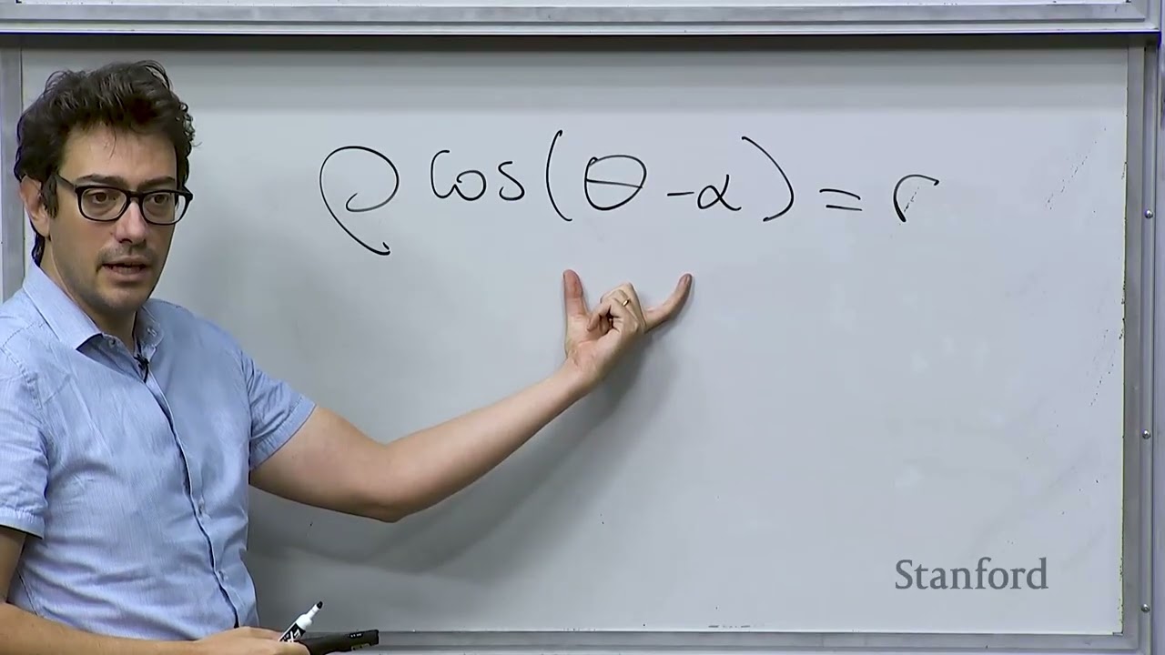
  • Polar line parameterization (ρ cos(θ - α) = r) eliminates the unbounded slope singularity inherent to Cartesian slope-intercept models and directly aligns with the native range-bearing output of LiDAR sensors. (13:09)
  • The sample size requirement for RANSAC line fitting depends solely on target confidence p and inlier ratio w (k = ln(1 - p) / ln(1 - w²)), keeping runtime invariant to total point cloud volume. (42:08)
  • The polar Hough Transform maps spatial points into bounded sinusoidal accumulator curves, enabling parameter-free line voting that avoids the numerical blowup of infinite Cartesian slopes. (53:11)
  • Classical recognition pipelines—including normalized cross-correlation template matching and Bag of Visual Words histograms—provided the structural foundations now learned end-to-end by modern deep neural networks. (76:18)

Detailed notes

## Background Published by Stanford Online on YouTube on October 18, 2026, this video features Lecture 12 of Stanford's AA274A course (Autumn 2019 edition), titled 'Principles of Robotic Autonomy | Classic Visual Recognition.' Delivered by Prof. Marco Pavone, an Associate Professor of Aeronautics and Astronautics at Stanford and Senior Director of Autonomous Vehicle Research at NVIDIA, the lecture covers information extraction and classical computer vision pipelines in robot perception.

## TL;DR Prof. Marco Pavone concludes the course's perception module by exploring how autonomous robots extract low-level geometric primitives and semantic scene understanding from visual data. He details line parameterization in polar form, formulating least squares fitting alongside classic segmentation algorithms including Split-and-Merge, Iterative End-Point Fit, RANSAC, and the Hough Transform. Transitioning to classic visual recognition, Pavone demonstrates template matching via normalized cross-correlation, multi-scale image pyramids with anti-aliasing filters, and the Bag of Visual Words framework, contrasting these handcrafted paradigms with modern deep learning approaches used in robotics.

## Atmosphere & style The lecture maintains an engaging, pedagogical, and conversational atmosphere, balancing rigorous mathematical derivations with relatable engineering humor and personal anecdotes about testing autonomous vehicles. Pavone interacts smoothly with student questions from the hall, guiding the room through geometric intuitions and practical trade-offs with unhurried clarity. Watching the session feels like sitting in an intellectually vibrant graduate seminar that seamlessly bridges foundational classical vision techniques with the modern reality of deep learning in robotics.

## Bulletin - [00:05](https://www.youtube.com/watch?v=GsIRJJ5sYoU&t=5s) Autonomous robot perception balances semantic depth against operational agility: high-speed vehicles require only minimal geometric models for localization, whereas complex manipulation tasks demand rich semantic representations. - [13:09](https://www.youtube.com/watch?v=GsIRJJ5sYoU&t=789s) Polar line parameterization (ρ cos(θ - α) = r) eliminates the unbounded slope singularity inherent to Cartesian slope-intercept models and directly aligns with the native range-bearing output of LiDAR sensors. - [42:08](https://www.youtube.com/watch?v=GsIRJJ5sYoU&t=2528s) The sample size requirement for RANSAC line fitting depends solely on target confidence p and inlier ratio w (k = ln(1 - p) / ln(1 - w²)), keeping runtime invariant to total point cloud volume. - [53:11](https://www.youtube.com/watch?v=GsIRJJ5sYoU&t=3191s) The polar Hough Transform maps spatial points into bounded sinusoidal accumulator curves, enabling parameter-free line voting that avoids the numerical blowup of infinite Cartesian slopes. - [01:16:18](https://www.youtube.com/watch?v=GsIRJJ5sYoU&t=4578s) Classical recognition pipelines—including normalized cross-correlation template matching and Bag of Visual Words histograms—provided the structural foundations now learned end-to-end by modern deep neural networks.

## Key takeaways - [00:05](https://www.youtube.com/watch?v=GsIRJJ5sYoU&t=5s) Information extraction exists on a trade-off spectrum between low-level geometric primitives used for agile localization and high-level semantic scene understanding required for complex task planning. - [03:18](https://www.youtube.com/watch?v=GsIRJJ5sYoU&t=198s) Geometric feature extraction decomposes into two sequential sub-problems: segmentation (determining which points belong to which primitive) and fitting (estimating the optimal geometric model). - [04:59](https://www.youtube.com/watch?v=GsIRJJ5sYoU&t=299s) Polar representation expresses lines as ρ cos(θ - α) = r or x cos α + y sin α = r, ensuring compact, bounded parameter spaces and avoiding vertical-slope singularities. - [18:17](https://www.youtube.com/watch?v=GsIRJJ5sYoU&t=1097s) Because range sensor uncertainty scales quadratically with distance (σ² ∝ ρ²), unconstrained least squares must be upgraded to weighted least squares with inverse-variance weights. - [27:31](https://www.youtube.com/watch?v=GsIRJJ5sYoU&t=1651s) The Split-and-Merge and Iterative End-Point Fit algorithms recursively partition ordered points at maximal orthogonal residuals until all sub-segments fall below an error threshold. - [33:04](https://www.youtube.com/watch?v=GsIRJJ5sYoU&t=1984s) RANSAC bypasses an exhaustive O(N²) search over point pairs by iteratively generating candidate lines from random samples and maximizing inlier consensus. - [42:08](https://www.youtube.com/watch?v=GsIRJJ5sYoU&t=2528s) The minimum iteration count for RANSAC is strictly governed by k = ln(1 - p) / ln(1 - w²), making computational effort independent of the total number of sensor readings. - [46:46](https://www.youtube.com/watch?v=GsIRJJ5sYoU&t=2806s) The Hough Transform leverages point-line duality by projecting spatial points into parameter space lines or curves that intersect at cells representing shared collinear parameters. - [53:11](https://www.youtube.com/watch?v=GsIRJJ5sYoU&t=3191s) Formulating the Hough Transform in polar space (α, r) bounds the accumulator grid across [0, 2π) and maximum sensor range, avoiding infinite slope bins. - [56:01](https://www.youtube.com/watch?v=GsIRJJ5sYoU&t=3361s) RANSAC is preferred in heavily corrupted environments with severe multi-path LiDAR outliers, whereas the Hough Transform offers reliable performance without extensive hyperparameter tuning in cleaner scenes. - [01:04:43](https://www.youtube.com/watch?v=GsIRJJ5sYoU&t=3883s) Classical object detection can be formulated as template matching using normalized cross-correlation, effectively computing a sliding vector dot product that peaks at 1.0 upon exact alignment. - [01:09:48](https://www.youtube.com/watch?v=GsIRJJ5sYoU&t=4188s) Handling scale variation requires image pyramids, which must incorporate Gaussian low-pass filtering before downsampling to prevent aliasing caused by violating the Nyquist sampling rate. - [01:15:02](https://www.youtube.com/watch?v=GsIRJJ5sYoU&t=4502s) The Bag of Visual Words model borrows from text processing by categorizing an image using a frequency histogram of quantized local feature descriptors matched against a dictionary. - [01:16:18](https://www.youtube.com/watch?v=GsIRJJ5sYoU&t=4578s) Modern deep learning replaces handcrafted templates and descriptors by automatically learning optimal visual representations from data, while executing the same underlying scene-decomposition principles.

## Detailed walkthrough ### [00:05](https://www.youtube.com/watch?v=GsIRJJ5sYoU&t=5s) Information Extraction and the Perception Trade-off

Prof. Marco Pavone opens the lecture by concluding the second module of the course on robot perception. The focus is specifically on the fourth step of the image processing pipeline: extracting information from sensor measurements (particularly cameras) to enable either robot localization (which will be covered the following week) or higher-level scene understanding for decision-making—such as determining whether a detected object is a human or an animal. The primary reference for this material is Chapter 4 of the textbook by Roland Siegwart and Illah Nourbakhsh (*Introduction to Autonomous Mobile Robots*).

Pavone highlights a fundamental engineering trade-off regarding environmental perception: autonomous robots do not always require an exhaustive, detailed understanding of their surroundings. In fact, a strict trade-off exists between the depth of semantic comprehension and the robot's operational speed and agility:

> “If you have a robot that is flying at very high speeds, maybe everything that you need is just to have a geometric understanding of the word but you really don't need to reason about the fine details of what what you have around the robot.”

Conversely, a manipulation robot that must pour water into a glass requires an advanced, structured model of the world. It must understand spatial relationships between objects to plan and execute a multi-step sequence of tasks. Pavone categorizes information extraction into two tiers: - **Low-level geometric features:** Primitives such as lines or circles, which provide the essential foundational geometry needed for robot localization. - **High-level features:** Semantic scene interpretation, such as identifying a table or recognizing specific objects, which is required for task planning in complex environments (e.g., preparing a dish or driving through a city).

```mermaid flowchart TD accTitle: Information Extraction Hierarchy in Robot Autonomy accDescr: Diagram illustrating the split between low-level geometric primitives used for localization and high-level semantic features used for task planning.

subgraph LowLevel["Low-Level Geometric Features"] Lines["Lines / Circles / Planes"] Localization["Robot Localization & High-Speed Agility"] Lines --> Localization end

subgraph HighLevel["High-Level Semantic Features"] Objects["Object & Scene Recognition"] Planning["Task Planning & Manipulation"] Objects --> Planning end ```

[03:18](https://www.youtube.com/watch?v=GsIRJJ5sYoU&t=198s) Geometric Primitives and the Two Sub-Problems of Line Extraction

Moving into geometric primitives, Pavone notes that in 2D systems robots typically extract lines and circles, whereas in 3D settings they identify surfaces such as walls and ceilings. In this lecture, the class focuses specifically on line extraction, as it serves as the foundational geometric primitive that students must implement for their final project and Problem 2 of their problem set.

Extracting geometric primitives breaks down into two core computational problems: 1. **Segmentation:** Determining which sensor data points belong to which specific primitive (e.g., partitioning a point cloud or edge map into distinct candidate lines). 2. **Fitting:** Given a cluster of points associated with a primitive, estimating the optimal mathematical parameters that best describe the underlying shape.

Pavone chooses to tackle these steps in reverse order: fitting is introduced first because it is mathematically simpler, followed by segmentation.

[04:59](https://www.youtube.com/watch?v=GsIRJJ5sYoU&t=299s) Line Parameterization: Cartesian vs. Polar Representation

To formulate the fitting problem in 2D, Pavone reviews standard line representations. While Cartesian coordinates define a line as $y = mx + b$ (with slope $m$ and intercept $b$), computer vision and robotics applications generally favor a polar parameterization.

Pavone explains how a point in the Euclidean plane can be located using polar coordinates $(\rho, \theta)$, where $\rho$ represents the Euclidean distance from the origin to the point, and $\theta$ is the counterclockwise angle between the positive $x$-axis and the segment connecting the origin to the point.

``` y | / | / line | * (x, y) = (\rho, \theta) | /| | \rho/ | | / | | / | | / \theta\ +--------*---- x origin P_0 \ / r \ / segment \perp line \ / * ```

To parameterize an entire line in polar terms, consider the line segment extending from the origin perpendicular to the line itself: - Let $P_0$ be the point where this orthogonal segment intersects the line at a $90^\circ$ angle. - Let $r$ denote the length of this normal segment (the perpendicular distance from the origin to the line). - Let $\alpha$ denote the angle of this normal segment with respect to the $x$-axis.

Any point lying along the line can be represented in polar coordinates by $(\rho, \theta)$. The geometric angle between the point's position vector and the normal segment is given by $(\theta - \alpha)$. Applying basic right-triangle trigonometry yields the polar equation of the line:

$$\rho \cos(\theta - \alpha) = r$$

Pavone checks with the room to ensure everyone follows the derivation. Using the angle subtraction identity $\cos(\theta - \alpha) = \cos\theta \cos\alpha + \sin\theta \sin\alpha$, this expands to:

$$\rho \cos\theta \cos\alpha + \rho \sin\theta \sin\alpha = r$$

Since standard Cartesian conversions give $x = \rho \cos\theta$ and $y = \rho \sin\theta$, substituting these relations produces the Cartesian projection:

$$x \cos\alpha + y \sin\alpha = r$$

- Every point $(\rho, \theta)$ lying on the line satisfies the normal form $\rho \cos(\theta - \alpha) = r$. - The pair $(r, \alpha)$ uniquely identifies any 2D line.

[13:09](https://www.youtube.com/watch?v=GsIRJJ5sYoU&t=789s) Addressing Singularities and the Advantage of Polar Form

A student raises an edge case: > “How do we deal with lines that go through the origin point in this construct?”

Pavone acknowledges that when a line passes directly through the origin, $r = 0$, making the normal direction $\alpha$ ill-defined or ambiguous. However, he emphasizes that the Cartesian form $y = mx + b$ suffers from a far more disruptive mathematical singularity: vertical lines require the slope $m$ to approach infinity ($m \to \infty$).

Pavone explains why this makes polar parameterization vastly superior for algorithmic estimation and data fitting: - In Cartesian coordinates, the parameter space for $m$ spans an unbounded interval $(-\infty, \infty)$, creating severe numerical instability during grid searches or optimization. - In polar coordinates, the parameter spaces are compact and bounded: the angle $\alpha$ strictly falls within $[0, 2\pi)$, and the radial distance $r$ is bounded by the finite physical dimensions or field of view of the sensor measurements.

[14:14](https://www.youtube.com/watch?v=GsIRJJ5sYoU&t=854s) Polar Line Representation and Least Squares Formulation

Prof. Marco Pavone resumes the discussion on representing lines in polar coordinates, noting that because an operational environment is naturally bounded, the distance $r$ from the origin to the line is always a well-defined number. He then frames the basic estimation setup: suppose a robot collects $n$ sensor readings, $(\rho_i, \theta_i)$ for $i \in \{1, \dots, n\}$, and knows ahead of time that they all belong to the same underlying line. In an idealized world, there exist line parameters $r$ and $\alpha$ satisfying:

$$\rho_i \cos(\theta_i - \alpha) = r$$

This yields a system of nonlinear equations that one could theoretically solve directly. In practice, however, real-world data is plagued by measurement noise, outliers, and sensor inaccuracies. Even when points physically originate from a planar surface like a wall, their measurements exhibit non-zero residual errors.

To cope with this, the line parameters must be estimated through optimization. The standard approach is to formulate an unconstrained least squares problem over the line parameters $r$ and $\alpha$ that minimizes the sum of squared discrepancies between the measured points and the candidate line:

$$J(r, \alpha) = \sum_{i=1}^n d_i^2$$

Here, $d_i$ represents the orthogonal distance from each measured point to the candidate line. As Pavone emphasizes, “Basically we're trying to find the line that best explains the point by minimizing the orthogonal distance between that line and each one of those points summing all those errors.”

```mermaid flowchart LR accTitle: Unconstrained Line Fitting Flow accDescr: Pipeline from raw polar sensor measurements to an unconstrained least squares optimization yielding line parameters r and alpha.

subgraph SENS["Sensor Data"] P["Points (ρ_i, θ_i)"] end subgraph OPT["Optimization"] C["Cost J(r, α) = Σ d_i²"] M["Minimize over (r, α)"] end subgraph OUT["Fitted Line"] L["Line Parameters (r, α)"] end

P --> C C --> M M --> L ```

[18:17](https://www.youtube.com/watch?v=GsIRJJ5sYoU&t=1097s) Noise Characteristics and Weighted Least Squares

A student in the lecture halls questions whether the formulation assumes there is no noise on the angle $\alpha$. Pavone clarifies that $\alpha$ and $r$ are merely the deterministic, underlying geometric parameters of the physical line itself. The noise resides directly in the measured quantities—the range $\rho_i$ and the bearing $\theta_i$ returned by the sensor (such as a LiDAR). Measurement errors in range and bearing induce an offset pushing the recorded point away from the true line, which the minimization of orthogonal distance attempts to counter.

The student follows up by drawing a comparison to Cartesian systems: in standard Cartesian regression, one typically assumes Gaussian error in $x$ and $y$ and runs least squares, and asks whether polar errors in LiDAR translate to equivalent Gaussian errors in $x$ and $y$. Pavone confirms: “The answer is yes. And we could actually do an error propagation analysis to see how those errors propagated into the final estimates that you compute. But we don't do it.” While a fully rigorous stochastic analysis could map the polar noise distributions into Cartesian distance uncertainty, it is omitted here for simplicity.

What cannot be ignored, however, is that measurement certainty varies drastically across space. In stereo vision and optical range sensing, uncertainty grows significantly for distant targets; specifically, variance scales with the square of the distance ($\sigma^2 \propto \rho^2$). This motivates upgrading unconstrained least squares to a weighted least squares formulation:

$$J(r, \alpha) = \sum_{i=1}^n w_i d_i^2 \quad \text{where} \quad w_i = \frac{1}{\sigma_i^2}$$

Points closer to the sensor have small variance $\sigma_i^2$, yielding high weights $w_i$, whereas distant, uncertain readings are heavily discounted.

[22:49](https://www.youtube.com/watch?v=GsIRJJ5sYoU&t=1369s) Closed-Form Solutions and Polar vs. Cartesian Coordinates

Despite the trigonometric nature of polar line equations, the weighted least squares objective admits exact closed-form expressions for the optimal $\alpha$ and $r$. Pavone points out that while the formula for $\alpha$ looks intimidating on the slides, it provides a direct, non-iterative computation required for the course's Problem Set 2. The formula for the distance $r$ is substantially cleaner:

$$r = \frac{\sum_{i=1}^n w_i \rho_i \cos(\theta_i - \alpha)}{\sum_{i=1}^n w_i}$$

Pavone explains the intuition behind this result: the geometric projection $\rho_i \cos(\theta_i - \alpha)$ represents the perpendicular distance of measurement $i$ along the normal vector at angle $\alpha$. If all weights are identical ($w_i = 1$), the denominator simplifies to $n$, turning $r$ into the simple arithmetic average of the projected distances across all sample points.

A student asks why they cannot simply convert everything to Cartesian coordinates and solve standard linear regression. Pavone details three distinct advantages of the polar representation: 1. **Numerical conditioning**: Cartesian line models ($y = mx + q$) break down for vertical or near-vertical lines where the slope $m \to \infty$. In polar form, $r$ and $\alpha$ remain strictly bounded and well-conditioned. 2. **Native sensor format**: Range sensors like LiDAR natively output ranges and bearings $(\rho_i, \theta_i)$. Fitting lines directly in polar space bypasses unnecessary preliminary conversions. 3. **Compatibility with subsequent methods**: The polar representation $(r, \alpha)$ directly matches the parameter space used by Hough transforms for line segmentation later in the pipeline.

As Pavone summarizes, “So it's a mixture of pedagogical reason, the type of measurements that you actually have, and the fact that there's a little bit more robust way of doing it.”

[25:48](https://www.youtube.com/watch?v=GsIRJJ5sYoU&t=1548s) The Segmentation Problem and the Split-and-Merge Algorithm

Having established how to fit a line when all points are guaranteed to come from a single segment, Pavone pivots to the harder front-end problem: line segmentation. A LiDAR scan generates hundreds or thousands of returns across a room. The robot does not receive point sets labeled by surface; it must determine autonomously which subsets of points belong to which physical structures. Distinguishing whether consecutive readings correspond to a single continuous wall or two separate walls meeting at a corner is critical for mapping and localization.

Pavone announces they will cover three primary algorithms for line segmentation, starting with the simplest: the **Split-and-Merge** algorithm. Using slides with custom illustrations—jokingly attributing the diagrams to his “skillful PowerPoint drawing skills”—he highlights the core challenge: while human vision effortlessly separates points into two distinct line segments, an algorithm must systematically discover these groupings.

The initial step of Split-and-Merge is straightforward: - Treat the entire collection of unclassified points as a single candidate segment. - Fit a baseline line through all points using the closed-form line-fitting equations just derived. - Identify the point with the largest orthogonal residual to determine whether a split is required.

[27:31](https://www.youtube.com/watch?v=GsIRJJ5sYoU&t=1651s) Line Splitting by Maximum Distance

Prof. Marco Pavone continues explaining line segmentation algorithms from range data. In the basic split-and-merge approach, the algorithm begins with the assumption that all points might belong to a single line, and fits an initial line through them. Next, it identifies the point having the maximum distance from that fitted line. If that maximum distance exceeds a preselected design threshold—such as 1 cm or 1 mm—the algorithm concludes that the point cannot belong to the fitted line. Consequently, the single line must be split into two lines: one passing through the first subset of points, and the other passing through the second subset.

```mermaid flowchart TD accTitle: Split-and-Merge Line Segmentation Logic accDescr: Iterative procedure for fitting lines and splitting them when points exceed a distance threshold. subgraph Step1["Step 1: Fit and Test"] A["Fit line through point set"] --> B["Find point with maximum distance d_max"] B --> C{"Is d_max > threshold?"} end subgraph Step2["Step 2: Branching"] C -- "Yes" --> D["Split set into two subsets at max point"] D --> A C -- "No" --> E["Freeze set as valid line segment"] end ```

The algorithm iterates over each subset. For a given subset, a new line is drawn, and the point with the maximum distance relative to that new line is computed. If the maximum distance falls below the threshold, the algorithm freezes that subset of points as belonging to the line. It then tests the remaining subsets until all points pass the threshold criterion. A student asks how the algorithm splits the points into a group of three and a group of four after identifying the furthest point. Prof. Pavone clarifies that points are kept in an ordered list, denoted as $L$, and indexed; that indexing determines the split. In response to a follow-up asking whether they are indexed along the line, he acknowledges that in his carefully constructed illustrative example, the points fall neatly into an array, whereas in realistic scenarios, data rarely exhibits such clean sequencing and patterning.

[30:06](https://www.youtube.com/watch?v=GsIRJJ5sYoU&t=1806s) Iterative End-Point Fit and Practical Challenges

Prof. Pavone introduces a common refinement of split-and-merge known as the *Iterative End-Point Fit* (IEPF) variant. Instead of running least squares to fit line parameters at every step, the algorithm simplifies the process: it connects the first point in the indexed list directly to the last point. It then identifies the point with the largest perpendicular distance from that segment. If that maximum distance exceeds the threshold, the set is split at that point. The procedure repeats recursively on the resulting subsets: connecting the first and last elements of each subset, testing the furthest point, and splitting further if necessary.

Once no further splits are possible, a final post-processing merge step combines adjacent segments that share very similar orientations into a single straight line, correcting over-segmentation aposteriori. When asked whether convergence depends on the chosen threshold, Prof. Pavone confirms that setting the threshold can be tricky: “So the concept is fairly easy, but getting it to work correctly is a bit hairy and you have a problem in your problem set to do exactly that.” Another student notes that the procedure relies heavily on how the initial array is ordered. Prof. Pavone agrees, pointing out that indexing can be based on range distance, spatial image bucketing, or other heuristics, and that balancing these moving parameters is what makes implementing the method challenging in practice.

- The threshold remains constant throughout the algorithm's execution. - Problem Set 2 requires students to implement and tune this segmentation method. - Algorithmic choices for point ordering include sorting by range distance or assigning points to image buckets.

[33:04](https://www.youtube.com/watch?v=GsIRJJ5sYoU&t=1984s) Introduction to RANSAC (Random Sample Consensus)

The practical challenges of split-and-merge motivate the introduction of RANSAC, which stands for **RAN**dom **SA**mple **C**onsensus. Prof. Pavone highlights RANSAC as one of his personal favorite algorithms due to its elegance: “This is really super simple to implement and super robust, and actually is one of my favorite algorithms.” It is a general randomized iterative method designed to estimate model parameters robustly even when the dataset contains significant numbers of outliers.

While introduced here in the context of 2D line fitting, Prof. Pavone emphasizes that RANSAC's applicability extends far beyond simple line segmentation: - Rejecting outliers when finding feature correspondences across pairs of images in stereo matching pipelines. - Fitting 3D geometric planes in depth and point cloud data. - Robust parameter estimation across broad computer vision pipelines.

[34:33](https://www.youtube.com/watch?v=GsIRJJ5sYoU&t=2073s) Line Fitting and Inlier Counting with RANSAC

Prof. Pavone walks through how RANSAC operates for line segmentation: 1. Two points are chosen at random from the dataset, defining a unique candidate line. 2. The distance from every other point in the dataset to this line is computed. 3. Points whose distance is below a threshold distance $\gamma$ are counted as *inliers*. 4. Two new points are chosen at random, defining a new candidate line, and the inliers are counted again. 5. This process repeats for a fixed number of iterations, and the line that accumulated the largest number of inliers is selected as the winning model.

Prof. Pavone walks through a numerical example on the board: one candidate line yields 9 inliers, another test yields only 7, and eventually a lucky pair aligns with the true structure, capturing a much larger consensus set. To guarantee finding the best line deterministically, one would need to evaluate every possible pair among $N$ points, requiring $\frac{N(N - 1)}{2} \approx O(N^2)$ combinations—an intractable computation for large datasets with millions of points.

```mermaid flowchart LR accTitle: Single Iteration of RANSAC for Line Fitting accDescr: Steps executed during each randomized trial of the RANSAC algorithm. A["Pick 2 points randomly"] --> B["Fit unique line"] B --> C["Compute distance to all points"] C --> D["Count inliers where distance < gamma"] D --> E["Update best line if inlier count is highest"] ```

[36:46](https://www.youtube.com/watch?v=GsIRJJ5sYoU&t=2206s) Determining the Required Number of RANSAC Iterations

Rather than searching through all $O(N^2)$ candidate pairs, RANSAC relies on probability to drastically reduce the number of iterations required. If one has prior knowledge—or an adaptive estimate—of the fraction of inliers in the dataset, denoted by $w$, one can determine how many samples are needed to ensure a successful fit with high confidence. For instance, knowing sensor resolution and the physical length of a 1-meter target line provides a rough expectation that there might be 100 true inliers among a point cloud of 1 million points. More advanced variations of RANSAC estimate $w$ adaptively during execution.

Prof. Pavone frames the core mathematical derivation: let $w$ be the fraction of true inliers in the total dataset, and let $p$ be the desired probability of success—that is, the probability of drawing at least one sample consisting purely of true inliers (such as $p = 0.99$ or $0.999$). The goal is to calculate the minimum number of iterations needed so that the probability of selecting two valid inliers is at least $p$, allowing the algorithm to terminate in far fewer iterations than an exhaustive $O(N^2)$ search. He sets up the proof by analyzing the probability of picking two inliers in a single random draw.

[39:36](https://www.youtube.com/watch?v=GsIRJJ5sYoU&t=2376s) Probability of Inliers and the RANSAC Failure Rate

```mermaid flowchart TD accTitle: RANSAC Trial Probability Logic accDescr: Flowchart showing the probability calculations for sampling inliers vs encountering failures across K iterations in RANSAC. subgraph SingleTrial["Single Trial Probabilities"] A["Inlier fraction: w"] --> B["Both points are inliers: w²"] B --> C["At least one point is an outlier: 1 - w²"] end subgraph MultiTrial["K Independent Trials"] C --> D["Failure after K trials: (1 - w²)^K"] D --> E["Require failure prob ≤ 1 - p: (1 - w²)^K ≤ 1 - p"] E --> F["Iterations needed: k = ln(1 - p) / ln(1 - w²)"] end ```

The probability analysis for line fitting using RANSAC begins with determining the likelihood of selecting two valid inliers in a single random trial. Letting $w$ represent the fraction of data points that are inliers belonging to the target line, and assuming random point selections are independent, the probability of choosing two inliers is $w^2$. Consequently, the complementary probability that at least one of the selected points is an outlier equals $1 - w^2$.

When a student asks whether this assumes we already know where the line is, Marco Pavone clarifies that we do not know the line's position at all: we hypothesize that an environmental line exists with some fraction of inliers, and we use RANSAC to detect it. If the algorithm terminates after repeated iterations finding only an insignificant number of inliers, that simply reveals no coherent line was present. Over $k$ independent iterations, the probability that RANSAC is completely "unlucky"—meaning every single draw fails to select two inliers simultaneously—is given by:

$$(1 - w^2)^k$$

Pavone emphasizes the importance of walking through this derivation, stating: “The reason why I go through this derivation is that RANSAC is a very important algorithm. So besides line fitting, it's used much more broadly. So I want to make sure that at least you're familiar with the basic concepts.”

[42:08](https://www.youtube.com/watch?v=GsIRJJ5sYoU&t=2528s) Practical Considerations, Parameter Tuning, and Autonomous Driving

Responding to a student who points out that $w$ depends heavily on environmental variables such as object distance, Pavone agrees that $w$ is merely a rough conceptual estimate used to choose an appropriate iteration budget rather than a known quantity. He jokes about how terrifying it might seem that safety-critical perception depends on such probabilistic heuristics: “I know it seems scary, right? That the life of a person on autonomous car depends on this, but it works.” He shares a personal anecdote from his time testing autonomous vehicles: when he took his wife for a ride, she was completely relaxed, admiring how smoothly the car drove, while he sat terrified because he knew the messy probabilistic algorithms operating under the hood. He warns the students that after taking this robotics course, they will be far less relaxed riding in self-driving vehicles than an uninformed passenger.

Students also query whether points could be filtered by spatial density before running RANSAC, or how multiple lines can be detected if RANSAC only maximizes inliers for one line. Pavone confirms that data can be pre-filtered using region-of-interest or density thresholds, and that the classic multi-line approach simply extracts the line with the most inliers, removes those points from the dataset, and re-runs RANSAC on the remaining points.

To guarantee finding a pair of inliers with a desired probability $p$ (such as $p \ge 0.99$), the probability of failing in all $k$ trials must be at most $1 - p$:

$$(1 - w^2)^k \le 1 - p$$

Taking the logarithm yields the iteration guideline:

$$k = \frac{\ln(1 - p)}{\ln(1 - w^2)}$$

The key insight is that the required number of iterations $k$ depends strictly on the inlier ratio $w$ and desired confidence $p$, but is completely independent of the total point cloud size $N$. For sensors like lidar that produce millions of points per second, this independence is vital. Furthermore, advanced variants of RANSAC adaptively estimate and update $w$ on the fly.

- Single-trial failure probability: $1 - w^2$ - Multi-trial failure probability after $k$ trials: $(1 - w^2)^k$ - Closed-form iteration estimate: $k = \frac{\ln(1 - p)}{\ln(1 - w^2)}$ - Total point count independence: $k$ does not scale with point cloud size $N$

[46:46](https://www.youtube.com/watch?v=GsIRJJ5sYoU&t=2806s) The Hough Transform and Dual Parameter Space

Pavone introduces the Hough Transform as an alternative segmentation technique that is conceptually clever and widely used. While RANSAC is randomized, the Hough Transform provides a systematic voting scheme in parameter space. In Cartesian coordinates, a straight line is represented by:

$$y = m x + b$$

For any specific measured point $(x_i, y_i)$, there are infinitely many candidate lines passing through it, defined by all pairs of $(m, b)$ satisfying $y_i = m x_i + b$. Rearranging this relationship into parameter space:

$$b = -x_i m + y_i$$

Thus, a single point $(x_i, y_i)$ in the spatial $(x, y)$ coordinate frame maps to a straight line in parameter space $(m, b)$, where the spatial point's coordinates dictate the slope $(-x_i)$ and intercept $(y_i)$.

```mermaid flowchart LR accTitle: Hough Transform Duality accDescr: Mapping between Cartesian coordinate space and the Hough parameter space. subgraph ImageSpace["Image Space (x, y)"] P1["Point (x_i, y_i)"] P2["Point (x_j, y_j)"] L12["Collinear Line"] end subgraph HoughSpace["Hough Parameter Space (m, b)"] LP1["Line: b = -x_i*m + y_i"] LP2["Line: b = -x_j*m + y_j"] Intersect["Intersection (m*, b*)"] end P1 -->|"Maps to dual line"| LP1 P2 -->|"Maps to dual line"| LP2 Intersect -->|"Defines parameters of"| L12 ```

When two distinct points $(x_i, y_i)$ and $(x_j, y_j)$ are considered, each maps to a different line in $(m, b)$ space. Because exactly one straight line connects two points in Cartesian space, their parameter-space lines must intersect at a unique coordinate $(m^*, b^*)$. This intersection point gives the slope and intercept of the line passing through both image points.

[51:00](https://www.youtube.com/watch?v=GsIRJJ5sYoU&t=3060s) Accumulator Grids and Practical Voting

To translate this duality into a line detection algorithm, the continuous parameter space $(m, b)$ is discretized into a 2D accumulator grid. Each data point casts "votes" by incrementing all grid cells $(m, b)$ through which its corresponding parameter line passes:

1. Discretize the parameter space $(m, b)$ into a grid of accumulator bins initialized to zero. 2. For each detected point $(x_i, y_i)$, trace the line $b = -m x_i + y_i$ across the grid. 3. Increment the count of every accumulator bin $(m, b)$ intersected by this line by one. 4. Identify candidate lines by locating accumulator bins containing prominent peaks (high vote counts).

Pavone explains why the votes in real datasets do not concentrate perfectly into a single cell with isolated ones elsewhere: physical measurement noise and sensor inaccuracy cause points that are collinear in the real world to deviate slightly in the image. This deviation smears the intersections across adjacent accumulator cells, producing a fuzzy cluster around the true parameter peak rather than an ideal sharp point.

[53:11](https://www.youtube.com/watch?v=GsIRJJ5sYoU&t=3191s) Polar Parameterization in the Hough Transform

A student raises a question about grid sizing and parameter bounds in the $(m, b)$ slope-intercept space. Prof. Marco Pavone agrees that slope $m$ is inherently problematic because it represents a tangent that approaches infinity as lines become vertical, making it difficult to set a bounded accumulator grid. Another student asks if the method generalizes well to 3D for planes, and Pavone notes that it generalizes “a little bit less” and is primarily used for 2D line detection.

```mermaid flowchart LR accTitle: Hough Transform Line Mapping accDescr: Mapping an image point into sinusoidal accumulator curves in polar parameter space

subgraph Cartesian["Image Space"] P1["Point (x_i, y_i)"] end

subgraph Parameter["Polar Parameter Space"] EQ["r = x_i cos(alpha) + y_i sin(alpha)"] ACC["Accumulator Array H[alpha, r]"] PEAK["Peak Cell (alpha*, r*)"] end

P1 --> EQ EQ --> ACC ACC --> PEAK ```

To resolve the infinite-slope dilemma, Pavone redirects the discussion back to the polar representation of a line: $$x \cos\alpha + y \sin\alpha = r$$ Given an observed point $(x_i, y_i)$, the set of all candidate lines passing through that point forms a sinusoidal curve in $(\alpha, r)$ parameter space rather than a straight line as in $(m, b)$ space. A student questions whether this assumes an equal probability of lines across angles $\alpha \in [0, 2\pi]$ compared to the tapering distribution of slope $m$. Pavone clarifies that the primary benefit is practical computability: - $\alpha$ can be uniformly discretized over a bounded angle interval with a fixed resolution. - $r$ is the perpendicular distance from the origin to the line, which can be upper-bounded using the known physical dimensions of the environment. - Because both $\alpha$ and $r$ are strictly bounded, the accumulator matrix $H$ operates on a well-defined finite grid, avoiding numerical divergence toward infinity.

[56:01](https://www.youtube.com/watch?v=GsIRJJ5sYoU&t=3361s) Accumulator Voting and Algorithm Comparison

Pavone walks through the step-by-step implementation of the polar Hough transform algorithm. For every detected edge point $(x_i, y_i)$ across each discretized value of $\alpha$, the corresponding $r$ value is computed via $r = x_i \cos\alpha + y_i \sin\alpha$. The accumulator matrix cell $H[\alpha, r]$ is then incremented by one ($+1$). Once all points and angles have cast their votes, the cells with the highest counts designate the detected lines. In an idealized two-line example, all generated sinusoids intersect sharply at two points in $(\alpha, r)$ space. In noisy real-world data, intersections spread into loose clusters, but peaks remain straightforward to extract.

Responding to a question regarding whether the user must know the number of lines in advance, Pavone explains that you do not need an exact prior count: “In general, yes, you have upper bound. I mean, in a reasonable structured environment will be difficult to have one trillion lines. But no, in principle, this algorithm finds all the lines that are out there.” Rather than fixing the count, one applies a voting threshold to select significant local peaks. When asked to contrast line-fitting methods (least squares, RANSAC, and Hough transform) in terms of speed and performance, Pavone observes that on modern processors, all three are fast, but their tradeoffs differ: - **RANSAC:** Highly robust against massive outlier ratios, such as those caused by severe sensor noise or multi-path lidar reflections; however, it requires tuning multiple parameters (sample size, consensus threshold, iterations). - **Hough Transform:** Statistically less rigorous and slightly less robust to extreme clutter, but nearly free of sensitive tuning. As Pavone summarizes: “If you are in a situation with a lot of outliers due to measurement noise or the environment that produces a lot of reflections for your lidars, so you get a lot of garbage, then RANSAC is the way to go. If you're in a relative clean environment, then Hough transform deserves a try.” - **Discretization Choice:** When pressed on choosing the angular resolution, Pavone notes that while grid discretization and peak detection thresholds are tuning parameters, typically “between 50 and 100 values for alpha is plenty.”

[01:00:42](https://www.youtube.com/watch?v=GsIRJJ5sYoU&t=3642s) Classical Object Recognition and Template Matching

Transitioning into the final segment of the lecture, Pavone introduces object recognition. He points out that while modern robotics relies predominantly on deep neural networks—the primary focus of the advanced companion course, AA274B—understanding classical computer vision prior to roughly 2012 provides crucial intuition for why deep learning became dominant. Object recognition broadly includes detection, classification, and scene segmentation; in AA274A, the term is used broadly to encompass identifying discrete semantic entities (e.g., distinguishing a person from a table or a dog) beyond purely geometric line or plane primitives.

Pavone explains that semantic recognition is exceptionally difficult because objects frequently occlude one another, appear at arbitrary scales and 3D orientations, and exhibit extensive intra-class variability: - Humans and monkeys share broad morphological features, requiring algorithms to differentiate subtle variations. - For upcoming problem sets, students will implement template matching—such as detecting a stop sign—to experience firsthand its limitations under scale and perspective changes. - For the class final project, which involves navigating a mock urban environment, students will be provided a pre-trained neural network as a “black box” because classical template matching and bag-of-words pipelines are not reliable enough for complex multi-class urban navigation.

Pavone introduces the simplest formulation—object detection, where the target's identity is already known and the goal is solely localization within a cluttered scene. Drawing an analogy to the picture-book game *Where's Waldo?*, he shows a slide crowded with diverse characters, noting that even when looking for a known visual pattern, search across dense distractors remains non-trivial, drawing laughter from the class as students scan the image to locate Waldo.

[01:04:43](https://www.youtube.com/watch?v=GsIRJJ5sYoU&t=3883s) Template Matching via Normalized Cross-Correlation

Marco Pavone connects object detection directly to linear filtering, explaining that an object can be treated as a template or filter mask that slides across an image. At each pixel location, the correlation computes a weighted combination of the filter values and the surrounding pixel neighborhood, effectively measuring local visual similarity. He reminds the class of the correlation formula: it generates an output image where each pixel's value is the weighted average across a neighborhood dictated by mask $f$.

To make this computationally concrete and align with the problem set, Pavone explains how the 2D operation is rewritten as a vector dot product. Consider a template matrix $f$ with rows $f_1, f_2, \dots, f_n$. By concatenating these rows, one constructs a single vector $f$. Similarly, for a patch centered at coordinate $(x, y)$ spanning the local pixel neighborhood, its pixel values are flattened into an image patch vector. Noting a slight notation clash on the slide where indices shifted, Pavone clarifies that this vector should carry coordinates $x, y$ to show explicit dependence on the mask's current center location.

```mermaid flowchart LR accTitle: Template Matching via Vector Dot Product accDescr: An image patch and template filter are flattened into vectors and normalized to calculate similarity via dot product. subgraph Vectors["Vector Representation"] T["Flattened Template Vector f"] P["Flattened Patch Vector I(x, y)"] end subgraph Correlation["Normalized Correlation"] NORM["Normalize Vectors to Unit Length"] DOT["Dot Product: f · I(x, y)"] end subgraph Output["Detection Result"] PEAK["Peak Score ≈ 1.0 (Object Match)"] end

T --> NORM P --> NORM NORM --> DOT DOT --> PEAK ```

The correlation is then simply the dot product between the template vector and the patch vector, which measures vector alignment. When both vectors are normalized, their dot product reaches a maximum value of 1 exactly when the vectors are identical:

> “So in particular if the two vectors are normalized the dot product is maximum when these two vectors are equal which basically induces us to consider a problem object detection as a problem of a normalized correlation whereby we do the correlation for for simplicity just expressed as a dot product but where we normalize it in order that if the neighborhood around $x$ and $y$ looks exactly like the mask $f$ then this dot product is equal to one which has the intuition that the filter that has the notion of a template exactly looks like the neighborhood around $xy$ which means that we have found Waldo.”

When asked by a student whether filters can be composed across scales and rotations, Pavone confirms this is possible. Displaying the actual output on a Where's Waldo puzzle, he highlights how sliding the template across the scene yields a sharp, isolated correlation peak at Waldo's exact location, allowing a bounding box to be drawn automatically. He underscores that “this is not PPT this is done for real,” praising normalized cross-correlation as an elegant, practical application of linear filtering.

[01:09:48](https://www.youtube.com/watch?v=GsIRJJ5sYoU&t=4188s) Image Pyramids, Nyquist Frequency, and Anti-Aliasing

The primary limitation of basic template matching is its strict assumption about object scale. If the camera gets closer to the scene, Waldo appears much larger, causing a fixed-size template to fail. To overcome scale sensitivity, the system constructs an image pyramid by rescaling the original input image across multiple resolutions (both upscaling and downscaling) and applying template matching independently at each level.

Downsampling presents an aliasing hazard. Pavone demonstrates this with a synthetic example interlacing an image of a mouse with an image of a small chick on alternating column lines. When naively subsampling by dropping every other column, the chick vanishes entirely:

> “If I just remove every other line the ones that were giving you the chicken then that is gone. So we miss information.”

He relates this artifact directly to signal processing principles: interlacing two separate images creates high spatial frequencies that violate the Nyquist sampling rate. In response to a student's observation that high frequencies should be capped off, Pavone confirms that applying a Gaussian blur acts as a low-pass filter, smoothing out the high-frequency transitions before downsampling. After Gaussian smoothing, subsampling produces an intact composite without missing features.

Upsampling requires interpolation techniques: - Nearest-neighbor interpolation - Bilinear interpolation (noted as particularly effective) - Bicubic interpolation

Pavone emphasizes that interpolation is itself formulated as a linear filtering operation. He notes that building image pyramids with subsampling and upsampling will appear in the problem set as an extra problem designated for graduate students, though undergraduates are encouraged to try it as well.

[01:15:02](https://www.youtube.com/watch?v=GsIRJJ5sYoU&t=4502s) Bag of Visual Words Representation

Pavone transitions from rigid template matching to the more flexible "bag of visual words" framework, designed for cases where an object cannot be captured by a single static template. Borrowing directly from document retrieval in text processing, this technique treats an image as an unordered distribution of basic visual elements:

> “So the idea of the bag of visual words is that we interpret images as a distribution of features also referred to as visual words.”

Under this framework, a predefined dictionary or codebook contains fundamental visual features. At query time, the visual words present in a new query image are identified and tallied into a frequency histogram. Classification or retrieval is accomplished by comparing this feature histogram against a database of histograms extracted from pre-labeled training images to find the closest match.

[01:16:18](https://www.youtube.com/watch?v=GsIRJJ5sYoU&t=4578s) Bag of Visual Words and the Deep Learning Shift

Prof. Marco Pavone wraps up the discussion on classic recognition pipelines, specifically the Bag of Visual Words model. He acknowledges that numerous practical questions remain open—such as how to build the visual dictionary in the first place or how to efficiently compare histograms against thousands of database images—but chooses to keep the explanation high-level. At its core, the method treats an image as a collection of local features, identified by a detector and characterized by a descriptor. These descriptors are mapped against a visual vocabulary to produce a frequency histogram of "visual words." Prof. Pavone highlights the design trade-off in building this vocabulary: it must be large enough to capture the visual diversity of the world, but if it becomes excessively large, matching becomes computationally intractable and prone to errors. The resulting histograms are then matched against reference database images to perform classification.

Prof. Pavone reflects on the timeline of computer vision, remarking how rapidly the field shifted away from these handcrafted representations. He notes that this bag-of-words framework was the de facto standard until about seven or eight years prior—the exact era when he was completing his doctoral studies. Today, neural networks have completely taken over both feature description and visual recognition. Yet, Prof. Pavone emphasizes that deep learning is not operating on completely alien principles: operations like template matching and decomposing scenes into basis elements are effectively still happening, but they are now learned automatically from data rather than engineered by hand.

```mermaid flowchart LR accTitle: Bag of Visual Words Pipeline accDescr: Pipeline showing local feature detection and description leading to a visual word histogram and final database classification. subgraph FeatureExtraction["Feature Extraction"] A["Input Image"] --> B["Detect & Describe Features"] end subgraph Quantization["Quantization"] B --> C["Map to Visual Vocabulary"] C --> D["Frequency Histogram"] end subgraph Classification["Matching"] D --> E["Compare to Database"] E --> F["Predicted Category"] end ```

- High-level mechanism: images are represented as frequency histograms of visual words matched against an indexed reference database. - Dictionary trade-off: large enough to represent arbitrary real-world scenes, but compact enough for efficient nearest-neighbor search. - The conceptual link to deep learning: “It's not a neural network does something completely different from what it was done before. It's just that what people were painfully doing in terms of coming up with all the right templates and so on is now basically implicitly encoded through learning into a neural network to the point that now this is the most reliable thing that you can use in order for object recognition and indeed what you will be using for your final project as I said as a black box.”

[01:18:22](https://www.youtube.com/watch?v=GsIRJJ5sYoU&t=4702s) Final Project Tooling and Looking Ahead to Localization

Turning to the practical aspects of the course, Prof. Pavone clarifies that students will treat neural networks as black boxes in their final projects—simply feeding an image in and obtaining an object category out. The deeper mathematical and architectural details of neural networks are deferred to the follow-up course, AA274B (Principles of Robot Autonomy II).

This session concludes the robot perception module of the class, which spanned camera models, 3D scene reconstruction, low-level primitive detection, and advanced visual recognition. Prof. Pavone maps out the schedule ahead: the following Tuesday begins the localization and mapping section, starting with the fundamentals of filtering theory. Finally, he mentions that graduate students will have an advanced guest lecture the following day focusing on modern computer vision techniques.

- Project implementation: neural networks will serve as off-the-shelf classification modules where an image produces a label. - Advanced coursework: deep learning internals and vision architectures are covered in AA274B. - Upcoming syllabus roadmap: next week transitions from perception to localization and mapping, beginning with filtering theory. - Graduate session note: a specialized lecture on modern visual methods is scheduled for the next day.

## Mentioned Marco Pavone, Roland Siegwart, Illah Nourbakhsh, Introduction to Autonomous Mobile Robots, Principles of Robot Autonomy, Where's Waldo?, Stanford University, NVIDIA, NASA Jet Propulsion Laboratory, Massachusetts Institute of Technology

## Video description For more information about Stanford’s graduate programs, visit: https://online.stanford.edu/graduate-education

Lecture 12 — Information Extraction and Classic Visual Recognition

Note: This lecture was recorded as part of the 2019 edition of the course. Course content, structure, assignments, and other materials may have changed since this recording. The course links below point to the most recent edition and may therefore differ from what is presented in the video.

Read the companion textbook, Principles of Robot Autonomy, free online: https://porabook.com

Follow along with the latest course schedule and syllabus: https://stanfordasl.github.io/PoRA-I

Speaker: Prof. Marco Pavone

Dr. Marco Pavone is an Associate Professor of Aeronautics and Astronautics at Stanford University and a Senior Director of Autonomous Vehicle Research at NVIDIA. Prior to joining Stanford, he was a Research Technologist in the Robotics Section at NASA’s Jet Propulsion Laboratory. Dr. Pavone received his Ph.D. in Aeronautics and Astronautics from the Massachusetts Institute of Technology in 2010. His research focuses on the analysis, design, and control of autonomous systems, with particular emphasis on self-driving cars, autonomous aerospace vehicles, and future mobility systems. He has been recognized with numerous awards, including the Presidential Early Career Award for Scientists and Engineers from President Barack Obama, the Office of Naval Research Young Investigator Award, the NSF CAREER Award, the NASA Early Career Faculty Award, the IEEE Kiyo Tomiyasu Award, the CSS Award for Technical Excellence in Aerospace Control, and the Early-Career Spotlight Award from the Robotics Science and Systems Foundation.

Full playlist: https://www.youtube.com/playlist?list=PLR9iNyexfIkk

#StanfordOnline #RobotAutonomy #Robotics #PhysicalAI

[Source](https://www.youtube.com/watch?v=GsIRJJ5sYoU)

中文简报

Pavone削减语义视觉以保障机器人高速机动性 自主系统在高速运行时必须舍弃精细的语义理解,转而采用基础几何基元,以防止计算瓶颈削弱车辆机动性。 Marco Pavone教授在课程感知模块的结语中,探讨了自主机器人如何从视觉数据中提取低层几何基元以及语义场景理解。他详述了极坐标形式的直线参数化,建立了最小二乘拟合公式,并介绍了包括分裂-合并法、迭代端点拟合法、RANSAC以及霍夫变换在内的经典分割算法。在转向经典视觉识别时,Pavone展示了通过归一化互相关实现的模板匹配、带有抗混叠滤波器的多尺度图像金字塔,以及视觉词袋框架,并将这些手工设计的范式与机器人领域现代深度学习方法进行了对比。 自主机器人感知在语义深度与运行机动性之间进行权衡:高速运行的车辆仅需要最简的几何模型来进行定位,而复杂的操控任务则需要丰富的语义表征。 (0:05) 极坐标直线参数化(ρ cos(θ - α) = r)消除了笛卡尔斜截式模型固有的无界斜率奇点,并直接与激光雷达传感器原生的距离-方位角输出相匹配。 (13:09) RANSAC直线拟合的样本量需求仅取决于目标置信度p和内点比例w(k = ln(1 - p) / ln(1 - w²)),这使得运行时间不受点云总数据量的影响。 (42:08) 极坐标霍夫变换将空间点映射为有界的正弦累加器曲线,从而实现免参数的直线投票,避免了笛卡尔无穷大斜率引起的数值激增。 (53:11) 经典识别流程——包括归一化互相关模板匹配和视觉词袋直方图——奠定了现代深度神经网络端到端学习的结构基础。 (76:18)

Reading summary

Prof. Marco Pavone frames robotic perception as an engineering trade-off between operational agility and semantic depth, presenting the mathematical foundations of geometric primitive extraction alongside classical visual recognition techniques. The Perception Trade-Off and Polar Parameterization (0:05) Robotic perception balances operational speed against the complexity of scene understanding. Fast-moving aerial systems require only low-level geometric primitives for localization, whereas complex manipulation tasks demand rich semantic representations to plan interactions. For 2D geometric extraction, lines serve as the foundational building block. While Cartesian slope-intercept equations suffer from unbounded parameters and numerical singularities as slopes approach vertical, polar line representations avoid these issues. Weighted Least Squares Line Fitting (14:14) Fitting geometric primitives from sensor readings involves estimating optimal parameters from noisy observations. Because sensors like LiDAR natively deliver range and bearing, fitting lines directly in polar coordinates maintains compact bounds and matches downstream algorithmic spaces. Furthermore, measurement variance scales quadratically with distance in optical and stereo ranging, requiring weighted least squares to heavily discount distant returns while prioritizing high-confidence near-field points. Line Segmentation via Split-and-Merge, RANSAC, and Hough Transforms (25:48) Before lines can be fitted, raw sensor returns must be partitioned into distinct geometric clusters. Split-and-merge algorithms and iterative end-point fits recursively bisect ordered point sequences around maximal residual points, though they remain sensitive to point sequencing and distance thresholds. By contrast, RANSAC isolates consensus sets through random sampling, requiring an iteration budget that depends solely on the expected inlier fraction and target confidence while remaining invariant to total point count. Alternatively, polar Hough transforms map points into sinusoidal curves within bounded parameter grids, accumulating votes to extract multiple collinear features without sensitive hyperparameter tuning. Classical Object Recognition and the Deep Learning Shift (60:42) Moving beyond geometric extraction, classic visual recognition identifies high-level semantic entities. Template matching executes normalized cross-correlations across image patches, though it requires multi-scale image pyramids coupled with anti-aliasing low-pass filters to manage scale variation. Bag-of-visual-words pipelines aggregate quantized local feature descriptors into frequency histograms to match against reference databases. Pavone notes that while deep neural networks have replaced these handcrafted pipelines as the de facto standard, modern architectures still fundamentally learn analogous filter matching and spatial feature distributions from data. While handcrafted representations provide the structural foundation for robot localization and classic recognition, their sensitivity to scale, clutter, and parameter tuning has led modern autonomy stacks to adopt pre-trained neural networks for complex semantic classification, deferring deep architecture internals to advanced coursework.

精炼阅读摘要

Marco Pavone 教授在斯坦福大学 AA274A 课程中阐述了机器人感知系统的分层架构与经典视觉识别方法,指出自主机器人在几何图元提取与高阶语义理解之间存在速度与复杂度的权衡,并系统解析了直线拟合、分割算法以及基于模板和词袋模型的经典目标识别机制。 感知需求权衡与二维直线极坐标表征 (0:05) 机器人感知系统并不总是需要穷尽环境中的所有语义信息。高速飞行的无人机通常仅依赖低阶几何图元(如线、圆或平面)即可实现定位与避障,而需要执行复杂操作的机械臂则必须建立高阶语义世界模型以完成多步任务规划。在 2D 几何提取中,提取过程由分割与拟合两个子问题构成。对于拟合而言,传统的笛卡尔坐标系方程 y = mx + b 在斜率趋向无穷大(即垂直线)时会出现数值奇异性,参数空间在区间 (-∞, ∞) 内无界。相对而言,极坐标参数化方程 ρ cos(θ - α) = r(即 x cosα + y sinα = r)将直线映射为距离 r 与法线角度 α。在极坐标系下,角度 α 严格位于 [0, 2π) 之间,r 则受限于传感器的物理视野与环境边界,具备紧凑且有界的参数空间。这不仅规避了数值发散,还直接贴合了 LiDAR 等测距传感器原生输出距离与方位的特性。 加权最小二乘直线拟合与闭式求解 (14:14) 在确定一组测距数据点同属一条直线的假定下,由于传感器测量噪声与离群点的存在,点集到直线的投影具有残差。通过构建无约束最小二乘目标函数,算法寻求使点到候选直线的正交距离平方和 J(r, α) 最小化。在实际光学测距和双目视觉中,测量不确定性随探测距离急剧上升,其方差与距离平方成正比(σ² ∝ ρ²)。因此,拟合过程采用加权最小二乘法,赋予近处高置信度采样点更高的权重 w_i = 1 / σ_i²,降低远距离噪声点对估计结果的干扰。尽管极坐标方程包含三角函数项,该目标函数依然能够推导出解析闭式解。其中参数 r 的闭式解表现为各测量点在法向量方向投影距离的加权平均数,为后续的实时计算提供了无须迭代的直接解法。 点集分割的三种主流算法对比与参数推导 (25:48) 从未标记的点云中识别出不同几何结构的分割阶段常采用三种主要算法。第一种是拆分合并算法(Split-and-Merge)及其变体迭代端点拟合(IEPF),该方法基于有序索引点集,通过递归寻找偏离线段的最大正交距离点并在超过固定距离阈值时进行二分拆分,最终合并方向相似的邻近线段,但其收敛效果严重依赖初始点排序与阈值设定。第二种是 RANSAC(随机抽样一致),通过随机选取两个采样点建立模型,并在距离阈值 γ 内统计内点(inlier)数量。假定内点比例为 w,单次采样同时抽中两内点的概率为 w²,经历 k 次独立试验全盘失败的概率为 (1 - w²)^k;若要求算法成功率达到 p(如 0.99),所需迭代次数 k 满足 k = ln(1 - p) / ln(1 - w²)。该迭代上限完全独立于点云总规模 N,使其在高噪与强多径反射环境中具备出色的鲁棒性。第三种是霍夫变换(Hough Transform),它将图像空间的边缘点映射为极坐标参数空间 (α, r) 中的正弦曲线,并在离散累加器网格上累加投票,通过局部峰值检测直线;其优势在于参数调节少,但在极端杂乱环境中的统计鲁棒性略逊于 RANSAC。 模板匹配与图像金字塔的尺度滤波机制 (64:43) 在语义目标识别领域,经典方法将已知物体的检测视为基于滑动窗口的线性滤波过程。通过将模板掩码与局部图像块展平为向量并归一化,两者之间的相关性转化为向量点积;当局部模式与模板完全吻合时,归一化互相关(NCC)达到理论峰值 1.0。然而,固定尺寸模板无法应对物理视距变化引起的尺度缩放。为了解决尺度敏感性,视觉系统通常构建多分辨率图像金字塔,在各个层级分别运行匹配。在此过程中,下采样必须遵守奈奎斯特采样定律;若在降采样前未消除高频空间信息,可能导致图像结构出现严重混叠假象。因此,流水线在抽取样本前引入高斯模糊作为低通滤波器,而在上采样时则运用双线性插值或双三次插值重建高频细节。 视觉词袋模型与深度学习的演进逻辑 (75:02) 当目标物体存在多视角、遮挡或非刚性形变时,静态模板匹配面临失效风险。经典视觉因此发展出视觉词袋(Bag of Visual Words)模型。该架构借鉴文本处理的文档检索思想,通过局部特征检测器提取描述子,将图像特征量化映射到预先构建的视觉词典中,统计生成无序的词频直方图,最后与标注数据库进行相似度比对实现类别分类。词典规模在表示丰富度与搜索计算复杂度之间存在严格权衡。Pavone 强调,2012 年前以手工设计模板与特征词典为代表的经典视觉方法已被现代深度神经网络全面替代。现代深度学习本质上并未颠覆底层逻辑,而是将过去繁琐的人工滤波与模式匹配过程,转化为由模型在端到端数据驱动下自动学习表征,从而大幅提升了复杂动态环境下的识别鲁棒性。 本讲座确立了经典机器人感知从底层几何图元拟合、点云分割到高阶特征匹配的完整数学与工程体系。虽然现代自主移动任务已普遍将深度神经网络作为物体分类的核心工具,但理解参数化稳定性、采样抗混叠及霍夫与 RANSAC 算法的统计推导,仍是构建可靠机器人位姿估计和感知流水线的理论基石。

Original transcript

[0:05] Today we're going to uh conclude the [0:09] second module of this class about robot [0:11] perception and in particular we're going [0:14] to focus on the fourth step of the image [0:16] processing pipeline that is the step of [0:19] extracting information that can be used [0:22] for either say localization as we will [0:25] see next week or for uh higher level [0:29] seen understanding in order to inform [0:31] decision making. Is an object a human or [0:34] an animal and so on and so forth. So the [0:37] goal of today is to learn how to extract [0:40] information from sensor measurements in [0:42] particular from cameras and the main [0:45] reference for this lecture is a chapter [0:48] 4 from the book from Siguar Nurbanka. [0:54] So as I said the goal is to extract [0:57] information information from one or more [1:00] sensors in order to uh generate a higher [1:04] level perceptation [1:07] or for uh decision making. Now it's [1:10] important to realize that autonomous [1:13] robots do not always need to have a very [1:17] uh good understanding of the world [1:20] around them. And actually there is a [1:22] trade-off between how much understanding [1:25] you want to have and the speed and [1:28] agility of the robots. If you have a [1:30] robot that is flying at very high [1:32] speeds, maybe everything that you need [1:35] is just to have a geometric [1:36] understanding of the word but you really [1:38] don't need to reason about the fine [1:41] details of what what you have around the [1:44] robot. On the other hand, if you want to [1:46] manipulate the world, for example, if [1:48] you want to pour water into a glass and [1:50] sun, then you need to have a much more [1:53] advanced understanding of the world [1:55] around you. You need to know what is the [1:57] relation of an object with respect to [1:58] another one in order to understand the [2:00] sequence of tasks that are needed in [2:02] order to accomplish your task. Having [2:05] said that, in uh on the topic of [2:08] information extraction, we um [2:12] distinguish between low-level features, [2:14] basically geometric features such as [2:17] lines or um circles and sun that can be [2:21] used to inform localization. The most [2:24] basic [2:26] uh uh capability for a robot in order to [2:28] move around. And then we consider higher [2:31] level uh high level features such as [2:36] recognizing a table or recognizing an [2:38] object which are useful for higher level [2:40] understanding which are useful for task [2:42] planning. If the robot has to do [2:44] something that is more advanced than [2:45] just moving around for example [2:47] accomplish a complex tasks such as I [2:50] know uh prepare a dish for you or uh or [2:55] even drive around a city and so on. So [2:59] today we're going to look at uh both [3:01] topics both topics. So how to uh detect [3:05] uh geometric primitives in the uh [3:08] environment and also how to detect [3:11] object and hence have a more detailed [3:15] understanding of a scene. Let's start [3:18] with geometric primitives. [3:21] Now the typical geometric primitives [3:23] that one may want to uh extract as I [3:27] said before are typically lines or [3:29] circles uh or in 3D for example walls [3:33] ceilings and so on. The toy problems [3:38] in order to extract geometric priv [3:40] primitives are for example in the case [3:43] of line segmentation in the in the case [3:46] of line extraction which points belong [3:48] to which line that's a problem of [3:50] segmentation and given associations of [3:52] points to a line how do we estimate the [3:55] parameters of the line that best fits [3:58] those points. Now in this class we are [4:01] going to focus specifically on line [4:04] extraction particularly because this is [4:06] one of the most basic geometric [4:08] primitive that you want to extract and [4:10] indeed this is geometric primitive that [4:12] you will be extracting for your final [4:14] project in order to achieve localization [4:18] accordingly problem two in your pet uh [4:21] focuses on line extraction as I said [4:24] this is what you'll be using for your [4:25] final project [4:28] as I said and this This is true [4:29] basically for all geometric primitives. [4:31] There is a problem of segmentation which [4:33] points belong to a given geometric [4:35] primitive like a line and two once you [4:37] have found that association how you find [4:40] the geometric primitive that best [4:43] explain the points that have been [4:44] associated to that primitive. So we're [4:47] going to look at these two steps in turn [4:49] and in particular we're going to look at [4:51] the second step first which is easier [4:55] and then we look later on at the first [4:57] step. [4:59] So let's start with the second step. The [5:02] problem of fitting in particular in the [5:04] case of a line in 2D similar arguments [5:07] generalized to uh 3D for example for [5:10] planes but just for simplicity for this [5:12] class we focus on lines. [5:15] Now everybody of you knows what an [5:18] equation of line of a line is. So if [5:21] you're into D [5:23] this is X this is Y and you have a line [5:27] the equation of a line in general is Y [5:29] equal MX + B. [5:31] So that's a usual equation of a line [5:34] typically for image processing we use a [5:38] different um parameterization of a line [5:41] and in particular the parameterization [5:43] of a line with respect to polar [5:45] coordinates. This is something that may [5:47] not be familiar with. So let's explain [5:50] what a line in a polar coordinates look [5:53] like. So you already know about polar [5:57] coordinates. We saw them earlier in this [5:59] class. Just to make sure that everyone [6:02] is on on the same page. So let's assume [6:04] that you have a point in the ukidian [6:07] plane. The coordinates you are used to [6:10] are the x and y coordinates. [6:15] But a different way to pinpoint where [6:18] that point is on the plane is in terms [6:20] of uh the distance of that point. Oops, [6:25] became [6:30] the distance of that point from the [6:32] origin which we denote as row and the [6:35] angle [6:38] uh theta [6:41] that the segment joining the point to [6:44] the origin forms with the x-axis. [6:48] If I tell you row and if I tell you [6:50] theta, you know exactly where the point [6:52] is, which means that row and theta are [6:54] valid coordinates in order to describe [6:56] each point in the plane. [7:02] So [7:04] then the question is we know how to [7:06] describe [7:09] a line in [7:12] cartisian coordinates. How do we [7:14] describe a line with respect to the [7:16] coordinates row theta? Meaning assuming [7:19] that we have a line [7:22] whose points are all identified [7:26] by polar coordinates row theta. What are [7:29] the parameters that identify this line? [7:33] In order to do so, [7:37] let's consider [7:44] the plot that we also have over there. [7:46] So, we're again given [7:51] the plane, then we're given a line. [7:56] So, let's call [8:00] B 0 and alpha. [8:05] So as you can uh see a line is uniquely [8:12] identified by the distance between the [8:16] origin and the point that the segment [8:19] orthogonal to the line from the origin [8:22] uh intersect the line and the angle of [8:25] that segment. Let's call the length of [8:28] the segment R. So here the [8:31] angle is 90°. [8:35] So if I tell you the length of this [8:37] segment again this is the segment from [8:39] the origin to the line that makes an [8:42] angle equal to 90° with the line. [8:46] If I tell you this distance and if I [8:48] tell you this angle I uniquely identify [8:51] this line. [8:53] Now then the question is what is the [8:57] relation between all the points [9:01] on this line with these two parameters [9:04] row uh sorry r and alpha that will give [9:07] us the equation of a line in polar [9:09] coordinates. [9:10] In particular let's take a general point [9:13] along the line with the coordinates row [9:17] and theta. [9:20] What's the relation between row and [9:21] theta and r and alpha? This is the [9:23] similar question that we will have for [9:25] what's the relation between the arbitary [9:27] point x y and on the line and the [9:30] parameters of the of the line m and b. [9:33] We already know that this relation is y= [9:36] mx + b. We want to find a similar [9:39] relation between row theta and r and [9:42] alpha. [9:44] Does it make sense? [9:49] All right. So [9:52] this length is row and this angle is [9:56] theta. All of this. So this angle [10:00] smaller one [10:03] this is a theta minus alpha. [10:06] So by using trigonometry [10:10] row times [10:12] cosineus of this angle is equal to r. [10:16] So row [10:18] cosinus of theta minus alpha is equal to [10:22] r. [10:25] And this is valid for every point on the [10:28] line [10:30] described with respect to polar [10:31] coordinates. [10:34] So [10:36] we can then define [10:39] a line with parameters r and alpha as [10:42] the locus of points such that those [10:44] points when described in polar [10:46] coordinates satisfy this equation [10:49] similar to what you would do in the [10:51] standard of cartigian coordinates. A [10:53] line is the locus of points such that [10:56] those points described in cartigian [10:58] coordinates satisfy this equation. [11:01] Does this make sense? [11:05] You don't seem convinced. You're [11:07] convinced. So, so [11:10] >> so or yes. [11:13] >> Okay. [laughter] Cool. All right. [11:16] [snorts] So, again, view this as the [11:20] polar coordinate representation of y= mx [11:24] + b. [11:28] Equivalently [11:34] by using the um and this will become [11:38] useful uh later on [11:41] by using the fact that cosinus of alpha [11:45] minus beta is equal to cosineos alpha [11:48] cosinos beta [11:51] plus sinos alpha sinus beta. [11:55] [snorts] [11:56] This equation can also be rewritten as [11:58] row cosineos of [12:01] theta cosinos of alpha [12:05] uh plus row sinos of theta [12:08] sinus of alpha. [12:13] So this is what [12:15] row cosine of [12:17] x. [12:18] >> Yep. So it's x cosine of alpha and this [12:21] is y sin of alpha equal r. [12:28] So basically this is how we go from the [12:31] equation of the line in polar [12:32] coordinates to the equation of the line [12:34] in xy coordinates. [12:38] Cool. All right. So all this to say that [12:42] uh in polar coordinates a line is [12:46] described in terms of the distance [12:48] between the point P 0 which is the [12:51] intersect intersection between the line [12:55] from the origin to the line orthogonal [12:58] to our line orthogonal to that line and [13:00] the angle that that segment forms. [13:06] Okay. So [13:09] we know we have now end points. Yes. [13:12] >> How do we deal with lines that go [13:14] through the origin point in this [13:16] construct? [13:19] You mean here this will be then with the [13:22] r equal to uh yeah this will be [13:25] not not well defined because we will not [13:28] have alpha but we have that singularity [13:30] also with the case of uh um [13:35] m because for example here m could go [13:39] all the way to infinity. [13:41] >> Yeah. sides. [13:44] But as we will see later, this [13:46] representation has an advantage with [13:48] respect to the cartigian advantage. In [13:51] particular, M is a number that can go [13:54] from zero to potential infinity. So when [13:58] we try to estimate from data this m, we [14:01] have to account for an infinite interval [14:03] for the slope. Instead, in the case of [14:05] the polar coordinate representation, [14:08] alpha is obviously between 0 and 2 pi. [14:11] And uh r is basically the distance of [14:14] the line from the origin. But since you [14:18] have a bound in terms of what [14:20] environment is, r is always a well [14:23] definfined number. And this is something [14:24] that we'll see we'll see later on. But [14:27] that's a good point. [14:29] Cool. All right. So now assume that yeah [14:33] here assume that now we have n points [14:37] row i theta i. [14:48] So we have n of those points [14:52] and we know that they all belong to the [14:54] same line. So there exist an r and alpha [14:59] such that uh row i cosinus of theta i [15:04] minus alpha is equal to r. So I give you [15:08] these end points. You know that they are [15:11] on the same line. We want to find r and [15:13] alpha. So this will be a system of [15:16] equations not linear but a system of [15:18] equations that you can solve for. [15:20] [snorts] Unfortunately due to noise [15:23] which could be due to measurement noise [15:26] outliers and so on. [15:29] Even if these points in reality belong [15:31] to the same line what we will measure is [15:34] something that has some residual some [15:37] error. [15:39] So the best we can do in order to [15:41] estimate the line meaning its [15:43] coefficient R and alpha is to find [15:46] coefficients R and alpha that best [15:52] describe how the points will fit that [15:55] line in terms of minimizing the residual [15:58] error. [16:01] Specifically [16:05] what we do is to is to form a cost [16:08] function [16:15] which is a function of the parameters of [16:17] the line. These are the two parameters [16:19] we want to find which is equal to the [16:21] summation from i = 1 to n the total [16:24] number of points over d i² the [16:27] discrepancy between [16:30] um [16:32] the equation of uh the line and what we [16:36] we actually have [16:42] >> this is just the discrepancy in r not [16:44] discrepancy [16:46] >> yeah well this DI basically accounts for [16:51] the [16:52] uh [16:54] distance of the point with respect to [16:58] the desired line. That's the meaning of [17:01] so basically we're trying to find the [17:03] line that best explains the point by [17:07] minimizing the uh orthogonal distance [17:10] between that line and each one of those [17:12] points summing all those errors. This is [17:15] a model obviously but usually the most [17:18] common model for line fitting. [17:22] So then the problem is to minimize [17:26] over R and alpha [17:32] this cost function [17:34] which you can see as a le squares [17:38] problem without constraints. [17:42] So here we're assuming that we uh [17:46] equally weight all the measurements. [17:48] Remember that the measurements are [17:53] the values row i's referred to as the [17:56] range or the distance to each point [17:59] something that a lateral sensor would [18:01] give you and the theta i which is the [18:04] bearing with respect to that point. [18:07] This is what you measure. You want to [18:09] find find the parameters R and alpha [18:12] that best explain those measurements in [18:15] terms of belonging to a line. Yeah. [18:17] [snorts] You're saying that there's no [18:19] noise on alpha in this model for you. [18:22] >> Well, implicitly you also can't for [18:26] noise in so the noise is really [18:31] we assume that we have noise in both. So [18:35] first of all [18:36] um the noise is not is neither in alpha [18:40] nor in R. So these are just the [18:42] parameter of the underlying line. The [18:44] noise is in row and beta which are the [18:47] quantities that we are measuring. So we [18:49] assume that because of the noise in row [18:52] and theta the end result will be a point [18:56] that is offset with respect to the line. [19:00] And then in order to find the line that [19:02] best fit those points, we try to [19:05] minimize the error in terms of the uh [19:08] distance of each point from that line. [19:11] >> So in a in a standard cartisian [19:13] measurement system, you kind of assume [19:15] there's a Gaussian error around X and a [19:17] Gaussian error around Y. And then we do [19:20] like the fitting of a line with like [19:22] these squares and it like minimizes [19:24] those errors some good way. [19:26] >> Yeah. And here we're working with the [19:31] we're now measuring things using like a [19:32] minor sensor, right? Which has error in [19:34] alpha and [19:35] >> yeah, typically with the lighter sensor [19:37] which are named [clears throat] so you [19:38] measure distance. [19:39] >> Does that still get you does that still [19:41] do errors in in alpha and distance still [19:44] translate to Gaussian errors in XY which [19:48] >> and yeah that's a good point. The answer [19:50] is yes. And we can we could actually do [19:53] an error propagation analysis to see how [19:56] those errors propagated into the final [19:59] estimates that you compute. But we don't [20:02] we don't do it [20:02] >> because the equation on the next slide [20:04] we go for slide that minimization [20:06] equation is minimizing for the gaussian [20:08] xy right [20:12] there's no real notion of xy here we are [20:14] really minimizing the uh distance [20:17] between a point and the line [20:22] >> so the question is how the gausian with [20:25] respect to row and theta transform into [20:27] a gausian for that distance that's what [20:30] we aren't minimizing which basically [20:32] leads so we could actually do a more [20:35] sophisticated stoastic analysis of the [20:38] foundation of what we're doing here but [20:42] we don't do it for simplicity also it's [20:43] not that important but what is important [20:46] to acknowledge as you were mentioning is [20:48] that uh there is an underlined notion of [20:50] uncertainty behind each measurement and [20:53] in particular we know for example for um [20:57] stereo engineing that measurements of [21:01] points that are farther away have more [21:04] uncertainty. In particular, the variance [21:06] increases with the square of the [21:08] distance [21:10] which [21:12] prompt us to actually weight the [21:15] different measurements. Basically give [21:17] more weight to those measurements that [21:19] are more certain. So points that are [21:22] closer to us and less weight to those [21:24] measurements that are farther away. [21:26] Practically what we do is to set up [21:28] weights wi equal to 1 / sigma i² that is [21:33] exactly what you were referring to the [21:35] uncertainty in the um [21:39] measurement that we have for a point [21:43] and consider then the weighted uh cost [21:47] function whereby if you see if we are [21:51] highly uncertain about a measurement [21:52] meaning that sigma is high then we give [21:55] less less weight for that measurement [21:57] when we do the le square fitting [22:00] procedure. [22:04] This is still a le square problem is a [22:06] weighted le square uh problem. Again [22:09] there are two things that uh we uh are [22:12] omitting here. The first thing is how [22:17] given uncertainty in row i and theta i [22:22] we come up with the characterization of [22:23] the uncertainty in sigma i [22:26] uh we are not uh doing that and we are [22:31] not doing all the say stoastic [22:33] interpretation of le squares so I'm just [22:36] uh [22:38] overlooking those issues and giving you [22:40] the uh high level intuition but from a [22:42] practical standpoint this This is what [22:44] you uh really need to uh know. [22:49] Now fortunately [22:51] this le square problem has a closed form [22:53] solution. They look horrendous but the [22:56] good news is that is a closed form [22:57] solution and this is really the equation [22:59] that you would use for probleming two in [23:01] your pet. In particular, the alpha that [23:06] optimizes that cost function is this [23:08] monster here. And the R, it is much more [23:12] benign uh formula here. Of course, if [23:15] the WIS are all the same, WIS are [23:19] actually equal to one, then the [23:21] summation of the WIS will be M. So this [23:24] would be uh basically the average of row [23:28] i= sen theta i over all the measurements [23:32] r which kind of makes makes sense right. [23:37] So just as for intuition row i cosine [23:40] theta i minus alpha. [23:48] So we had a line we had the segment is [23:51] perpendicular to the line. This was [23:53] alpha. Uh so this is a point on the line [23:57] with the coordinates row and theta and [24:01] is r. So row cosine theta minus alpha is [24:07] this distance. [24:12] So basically the distance with respect [24:14] to the line. And so we take r as the [24:17] average of those distances [24:20] which kind of makes sense. [24:24] Yeah. Why don't we just can't we just [24:27] solve this in cartigian? [24:32] >> Yeah. So the only thing is that uh in [24:34] cartisian coordinates you could but in [24:38] cartigian coordinates the problem is a [24:40] little bit less well conditioned because [24:43] m the slope can be a number that could [24:46] be very large and two because I would [24:49] use this polar represent. So there are [24:52] three reason that second typically your [24:55] measurements in terms of range [24:57] measurements are in the form of rows and [24:59] thetas. So you don't get x and y from a [25:02] ladder you get row and theta. So is you [25:04] could do the transformation obviously [25:06] but is better to just go straight from [25:08] the measurement to the line fitting. [25:10] Three, I will use the uh polar [25:13] representation of a line in order to [25:16] also solve the segmentation problems by [25:19] using Q transform that we're going to [25:20] discuss in a few slides. So just to for [25:24] ease of explanation, I prefer to do [25:26] everything in polar coordinates. But [25:28] [snorts] yes, in principle you could do [25:30] it in XY as well. [25:34] Does it address your question? [25:35] >> Yeah. So it's a mixture of pedagogical [25:39] reason uh the type of measurements that [25:41] you actually have and the fact that [25:44] there's a little bit more robust way of [25:45] doing it. [25:48] All right let's go to step number one [25:50] light sementation. So so far we have [25:51] assumed that we have a bunch of points [25:54] we know that they all belong to a line [25:56] and then we want to find the [25:57] coefficients of that line. We use polar [25:59] coordinates for a number of reasons and [26:00] I just explained. Of course, if you're [26:02] really against polar coordinates, then [26:04] you can use cartitionian coordinates. [26:07] The first problem is okay, but who tells [26:09] you whether a bunch of points belong to [26:12] uh a given line? What you get from [26:15] ladders are a bunch of row eyes, theta [26:19] eyes, which is very large. Which point [26:22] belongs to which line? [26:25] And that's tricky. And that's very [26:27] important because of course for [26:28] localization you want to understand [26:30] whether that wall is the same on that [26:32] wall or there two different walls with [26:35] an angle between them. So we're going to [26:37] look at the three uh main methods for [26:40] line segmentation [26:42] um that are relatively simple but still [26:46] require a little bit of explanation. So [26:48] the first one which is really really [26:51] simple is referred to as a split and [26:54] merge. [26:55] The deal split and merge is best [26:57] illustrated by um [27:01] through my skillful PowerPoint uh [27:05] drawing skills. Uh so let's assume that [27:08] we have a bunch of points. Now it's a [27:10] segmentation problem. We don't know [27:11] which point belongs to which line. As a [27:14] human you will say okay probably this is [27:16] a line and this is a line. This is what [27:19] we want to do with the algorithm. All [27:21] right. So we had this bunch of points. [27:23] So the first thing that we do is just to [27:26] fit a line through all of these points [27:29] by using the same algorithm that I [27:31] explained before. So we assume okay [27:34] maybe all of them belong to the single [27:36] line and that's what we do. We fit this [27:39] line. Then we uh look at um the point [27:46] that has a maximum distance from the [27:49] line. In this case, this will be the [27:52] probably yeah probably this one. This [27:55] will be the point that has a maximum [27:57] distance to the line. [27:59] So then we say okay if this maximum [28:02] distance is above a design threshold say [28:07] 1 cm or 1 millm that's a threshold that [28:09] you decide. If this distance is above [28:12] the threshold then we say okay this [28:14] point cannot really belong to that line [28:17] which means that I have it to split this [28:20] line into two lines. So one that will go [28:24] through this set of points and the other [28:27] one that goes through that set of point [28:31] so that's what we do and then we [28:33] iterate. So this is an iterative [28:34] algorithm. Now I have this subset of [28:36] points. I redraw a line. I compute I [28:40] find the point that has maximum distance [28:43] with respect to the line in this case [28:44] this one and I say is this distance less [28:47] than the acceptable threshold in this [28:49] case it is so then I freeze this set of [28:52] points as belonging to the same line I [28:54] go to this other one and again here all [28:57] the points pass the threshold test and [28:59] then I'm done yeah [29:00] >> so you identified the one that was [29:02] furthest away from the first person [29:04] >> but then how did you split the points [29:06] into the group of three and a group of [29:08] four. [29:08] >> Yeah. So basically I have a order list [29:11] of points that I define as uh where is [29:15] it L [29:17] >> and then they are indexed. So I use that [29:20] indexing in order to split them. [29:22] >> So are they along the line? [29:24] >> Yeah. No along the line. So basically I [29:27] have at the beginning I just have a [29:29] bunch of points and I just put them in [29:31] an array. [29:33] So just hypothetic. [29:35] Okay. [29:36] >> Oh yeah. See this is a very carefully [29:39] constructed case so that into iteration [29:41] it stops right. No no you're right. In [29:43] general I don't have this very nice [29:45] sequencing and this very nice pattern [29:47] >> such a way that you like have you split [29:50] the points like in the not correct way. [29:53] >> Well but then you will keep uh splitting [29:55] at least until you don't have these [29:57] weird things. There is another uh step [30:01] >> that's the first [30:02] >> exactly. So I have another example that [30:06] maybe addresses that a little bit [30:07] better. So this is a refinement of split [30:10] and merge that is referred to as [30:12] iterative endpoint fit variance. So what [30:14] you do is it's basically an [30:17] simplification of the previous um [30:21] algorithm whereby instead of doing le [30:23] squares in order to compute the [30:25] parameters of the line you just merge. [30:28] So you just have a bunch of points that [30:30] you have ordered somehow [30:33] and then you you connect the first point [30:36] according to your indexing to the last [30:38] point. In this case will be these two. [30:42] Same deal as before. We compute the [30:44] point that is that has the farthest [30:46] distance and then we split. [30:52] And then oops [30:54] and now for this subset of point we [30:56] compute another line [30:59] by uh connecting the first and the last [31:02] element of that set. We compute the [31:04] point that is the farthest away. [31:07] And this is again above the threshold. [31:09] So we split. [31:11] I get here. So here no more splits are [31:14] possible and then there is final [31:17] post-processing step whereby we just [31:19] merge and we have a straight line. [31:23] This is exactly the case that because of [31:25] the splitting procedure we introduce two [31:28] lines that were very similar with each [31:30] other. So we corrected that aposteriori [31:32] with the emerge procedure. [31:36] So of course there are a lot of moving [31:37] parameters in this thing. So getting it [31:39] to work correctly. So the concept is [31:42] fairly easy but uh getting it to work [31:45] correctly is a bit hairy and you have a [31:47] problem your pet said to do exactly [31:49] that. [31:50] >> So uh does the convergence uh happens [31:54] based on the amount of threshold you [31:56] set? [31:57] >> Oh yeah of course uh that's why I'm [31:59] saying it's a bit hairy because [32:00] depending on the threshold you might get [32:03] results that are really awkward and as [32:06] you will see in the second problem of [32:07] the pet. So yeah, that requires a little [32:10] bit of experience. [32:12] [clears throat] [32:13] >> The threshold remains the same [32:15] >> typically. Yes. [32:16] >> Yeah. [32:19] >> This felt like it was really dependent [32:21] on on the indexing of of that. [32:24] >> Yeah. [32:26] >> So how how do you go about choosing the [32:29] right index or or how how do you go [32:32] about constructing that initial array? [32:34] Yeah, there are a lot of moving there [32:36] are a lot of algorithm decisions. So one [32:39] for example would be to uh index them in [32:42] terms of their uh range distance [32:46] or you just put a buckets in terms of [32:48] where they are in the image. Basically [32:50] there are countless variations of how [32:52] you can do it. We provide you an example [32:54] in the pet 2 but you're right. So as I [32:57] said the idea is simple but making it [33:00] work correctly is not so simple which [33:02] actually [33:04] uh give rise to the second algorithm [33:05] that I want to mention bransack. This is [33:07] really super simple to implement and [33:10] super robust and actually is one of my [33:12] favorite algorithms is simple as I said [33:16] very robust ransack indeed is an idea. [33:19] So ransack first of all stands for [33:21] random sample consensus and is a a very [33:26] general algorithm that allows you to [33:29] estimate in the robust way parameters of [33:31] a model even in the presence of [33:32] outliers. So I'm using ransack for the [33:35] specific purpose of uh segmenting points [33:40] uh on a line but ransack can use much [33:44] more generally in order to find the [33:46] correspondences between points across [33:48] different images finding planes in the [33:51] 3D images and so on. So the ransa [33:53] concept per se is very very general. Um [33:57] so for example when you want to do [34:00] stereo matching and you have to find [34:02] correspondences between [34:04] um [34:06] two images then [34:09] most of the uh image processing pipeline [34:12] out there use ransack in order to reject [34:15] outliers and we'll see in a second how [34:17] uh that work but anyway the idea of [34:21] ransack is to use an iterative [34:23] randomized method in order to estimate [34:26] parameters by rejecting outliers. Let's [34:29] look at how it works for the case of [34:31] land segmentation. [34:33] So we have a bunch of points here. As a [34:36] human, you might argue that this [34:38] probably corresponds to a line. This [34:41] maybe is also a line. [34:44] So the way that the ransack algorithm [34:45] works is extremely simple. You take two [34:48] points [34:50] and then you computed the line that goes [34:52] through those those two points. Of [34:53] course, there is only one line that goes [34:54] through through the those two points. [34:57] And then you compute the number of [34:58] inliers, meaning the numbers of a point [35:01] that are within a distance, how do we [35:03] call it here? Gamma maybe the number [35:07] that go yeah that that are within a [35:09] distance gamma from that line. [35:12] And then I select other two points and [35:14] then I compute the number of in liners [35:16] and I do that a certain number of times [35:19] and at the end I choose the line with a [35:21] maximum number of iners. So the way it [35:24] works as I said you take two points like [35:27] for example this red point here and this [35:28] red point here you compute the line that [35:31] goes through them you compute the [35:33] inliers [35:36] meaning those points whose distance is [35:38] below a given threshold. So here I'm [35:40] computing all the distances. I only keep [35:42] the points whose distance is below a [35:45] given threshold. This is a set of liars. [35:47] So for example here I have 1 2 3 4 6 7 8 [35:50] 9. So this line has nine in liars. [35:55] I do it for these other two points. And [35:58] here I have three seven liars. Keep [36:02] doing that. Keep doing that until I'm [36:04] lucky. I pick these two points and I get [36:06] a big number of liars. [36:10] At the end I choose the line that has [36:13] the largest number of inliers. In [36:16] principle [36:17] in order to be exhaustive you should [36:20] consider all possible pairs. [36:23] So you have assume that you have in [36:25] total n points. So how many pairs you [36:28] will need to consider in total? Oops, [36:31] the answer is [snorts] already there is [36:33] n * n minus one over two because of [36:36] course the order with which you pick the [36:38] first point doesn't matter [36:42] which in general is very large. [36:46] So the idea of ransack is that you and [36:49] again this is a very general idea that [36:50] goes beyond the line fitting. It's not [36:53] that you have to select all possible [36:56] combinations but if you have a little [36:58] bit of a priority information in terms [37:01] of how many inlers you should expect for [37:04] a given geometric primitive you can [37:06] dramatically decrease the number of [37:08] points that you need to consider. How? [37:11] Let's assume that we have at least a [37:15] rough estimate [37:17] of [37:19] the percentage number of inliers that um [37:23] a geometric primitive uh will have. For [37:27] example, if you look at a line that is 1 [37:30] m long and you have a given resolution [37:32] for your ladder, you maybe have a good [37:34] sense that maybe the number of liar in [37:36] liar should be maybe 100. So 100 total [37:39] liars. If you have 1 million points that [37:41] gives you the fraction of a liar that [37:43] you should expect. [37:45] So this is something that often times [37:47] you have even if you don't have there [37:49] are more advanced version of ransack [37:51] that are capable of identifying W. So [37:54] the percentage of in liars in an [37:56] adaptive way. So basically you will [37:58] learn it as you um proceed with RNA. So [38:03] in particular let's assume that W the [38:05] fraction of inliers is something that we [38:07] either know or we have a good estimate [38:10] of it. So W is a fraction of in liars [38:15] and then let's assume that so this is a [38:17] randomized algorithm. Let's assume that [38:19] we have a desired probability [38:22] of finding a set of points that is free [38:26] of outliers. So that probability P for [38:28] example could be 99%. [38:32] So we want to run ransack a number of [38:35] times such that with probability at [38:37] least 99% I select two points that are [38:41] in layers [38:44] and this is again a design parameter you [38:46] can set it 99.9% as you want the [38:50] question is given the knowledge of the [38:53] fraction of liars and given the desired [38:56] probability of finding two points that [39:01] are are indeed in liars. What is the [39:04] number of times that I needed to run [39:06] ransack in order to find two iners with [39:09] probability at least 99%. [39:14] The reason why we're doing that is [39:16] because we want to run ransack a number [39:18] of times that is much lower than capital [39:21] n square. [39:23] To answer that, we just need to do a [39:26] little bit of probability. So the [39:29] probability of uh [39:33] of selecting two inlers so two point [39:36] that belong to that line [39:38] assuming that um the way we select [39:42] points is independent is [39:46] w square both points [39:49] in liar. [39:53] Yep. [39:56] the line or do you want to bend the line [39:57] in your chicken? [39:59] >> No, no, we don't know where the line is. [40:01] >> So, we know that there is a line. I [40:03] mean, we assume that there is a line and [40:05] uh we assume that there are some liars [40:07] along that line, but we don't know which [40:09] of them. [40:09] >> So, you're saying there is a line [40:11] already and you're choosing random [40:12] points in mind. [40:15] >> Yeah. We're trying to find a line. So, [40:17] we assume that there is a line in [40:19] environment and we run that run that [40:21] we're trying to find it. I mean it might [40:23] be the case that after we run ransack a [40:25] number of times we find a number of [40:28] liars that is very small which means [40:30] that basically there is no line in your [40:31] environment that is fine too but the [40:34] question is if there is a line can we [40:36] find it after running ransack a given [40:39] number of times with probability at [40:41] least 99%. [40:43] But of course if there is no line then [40:45] the ransack would not find that line. [40:48] So the probability that both points are [40:50] in liar is when when you select them the [40:54] probability that both points are in [40:56] liars will be w. [40:59] So the probability that at least [41:04] [clears throat] [41:04] one of them [41:07] is not an inar [41:13] is equal to 1 - w². [41:16] So what is the probability that after k [41:19] times that you run ransack you don't [41:21] pick two points that are in layers. [41:25] So the probability [41:28] how do we call it there? Ransack never [41:30] selects [41:34] okay ransack is unlucky. [41:38] Unlucky means never selects two points [41:40] that are both in layers. Is 1 minus W [41:45] square to the power of K [41:49] is unlucky after K trials [41:55] 1 - W square. The reason why I go [41:58] through this derivation is that Box is a [41:59] very important algorithm. So besides [42:01] line fitting, it's used much more [42:03] broadly. So I want to make sure that at [42:05] least you're familiar with the basic [42:06] concepts. [42:08] Doesn't depend on a lot about your [42:10] environment like like how far the object [42:13] is. [42:13] >> Yeah, absolutely. That's why W is really [42:16] a rough estimate. It's [clears throat] [42:17] like a conceptual construct that you use [42:20] in order to get a sense of how many [42:22] iterations you may need. But yes, you [42:25] never know W exactly. You just have some [42:28] estimate that you use to guide your [42:30] selection number of runs iterations. [42:35] I know it seems scary, right? that uh [42:37] the life of a person on autonomous car [42:39] depends on this but but it works. [42:43] >> So that point cloud you showed us and [42:45] all the points you could see as a human [42:48] that there's a line of points that was [42:49] denser than the rest of them. [42:52] >> Denser means that there are more in [42:54] light. Yeah. [42:55] >> Yeah. It would it be possible to cut [42:57] down points? You have to check with [42:59] ransack by only considering points that [43:02] are in a certain density threshold. So [43:04] like you don't [43:06] >> you could I mean you could better inform [43:08] ransack in order to tell Ransack to [43:10] focus on some regions? Certainly true. I [43:12] mean again ransack you have zillions of [43:15] variations. This is really the most [43:17] basic version of it. [43:19] >> Just based on the version you presented [43:20] won't ransack only ever find one line [43:22] the data provided? [43:24] >> Yes. Because we just pick the maximum [43:28] number of layers. So then what you would [43:29] do would be to remove all of these and [43:31] then run again to find our line. Yeah. [43:35] So coming back to the equation of uh [43:38] well is this thing works. So I remember [43:40] that when I first gave a rides on the [43:42] autonomous car that I was working on uh [43:45] a few years ago and my wife was running [43:48] on it was sitting on it. She was very [43:50] fine and oh wow this works very well and [43:52] I was scared to death because I knew [43:54] that this was all the thing under the [43:56] hood going. So the point being that [43:58] after this class if you happen to ride [44:00] an autonomous car you'll see that you [44:03] are much less relaxed about a person [44:05] that is not knowledgeable about what is [44:07] what there is behind. Yep. Anyway but [44:11] actually this works pretty well in [44:12] practice. So even though we make all [44:14] this approximation is a very robust [44:15] algorithm. In particular let's assume [44:18] that we are confident about the w value. [44:24] So the question is how many [44:27] uh iterations you need in order to find [44:30] a couple of iners. So a pair of liars so [44:32] that actually you have a line. Well as k [44:36] grows larger this quantity goes uh [44:41] monotonically and synthetically to zero [44:43] which means that as k becomes larger and [44:45] larger the probability that you don't [44:47] get to points become lower and lower. In [44:50] pro in particular, you want to find um a [44:56] pair of liars with probability at least [44:58] 99% say which means that you want the [45:01] probability of not finding the liar to [45:03] be less than uh 1%. So you run [45:08] uh runs until 1 minus p is greater than [45:14] or equal to 1 - w^ square to the power [45:17] k. And you know that there is a k that [45:20] is large enough such that this is true [45:22] because you know that as k goes to [45:24] infinity this goes to zero. [45:30] In particular basically you choose the k [45:34] such that this is an equality. It's not [45:36] really an equality because of course um [45:42] you may not find a k precisely that [45:44] makes this equal to 1 minus p. But just [45:46] for simplicity assity. [45:49] So you then consider a number of [45:52] iterations that is equal to log 1 - p [45:54] over log 1us w^ square. [45:57] Again this is basically guideline that [45:59] you use in order to tune your algorithm. [46:02] The important point here is that kar [46:04] depends on w but not on n [46:08] which means that in general with ransack [46:10] you need a number of iterations that is [46:12] much lower than the total number of [46:14] points. Since with lighters you have [46:16] millions of points that is a very [46:18] important concept. Second of all there [46:21] are more advanced versions of ransack [46:23] that actually retune uh the W in an [46:26] adaptive way. [46:31] All right any questions here? Again [46:34] ransack's useful for light fitting but [46:36] much more useful broadly. So if you [46:38] stick with the feed robot autonomy it's [46:40] very likely that you will stumble upon [46:42] ransack uh in the future. [46:46] Third method for segmentation Q [46:49] transform this is a very cute uh idea [46:52] and also quite widely used. So again the [46:56] idea is that we have a bunch of so you [46:59] see that we have increasingly more [47:00] refined ways of doing it. Of course the [47:03] more refined your method is more [47:04] computation you need to do. So same [47:07] problem we have bunch of points we want [47:09] to find uh whether there is a line that [47:12] goes through those points. [47:15] So the idea of the hue transform is [47:19] simple but very clever [47:24] that is that as we discussed before [47:29] a line in cartisian coordinates is [47:31] described as y= mx + b. [47:35] Okay, [47:37] which means that if I give you a point [47:40] with coordinates x i and y i, [47:45] what is the set of possible lines that [47:48] can go through that point will be this [47:51] line, this line, this line, this line [47:54] and so on. And in particular, [47:57] the set of lines that go through that [47:59] point is the set of values m and b's [48:03] such that y i equal mx i + b. [48:09] Which basically mean that [48:14] every point [48:18] xy [48:21] induces a set of possible values for the [48:26] line a line that goes through that uh uh [48:30] through that point. [48:33] Specifically, [48:37] the parameters of the line that go [48:39] through that point are related through a [48:42] linear equation. And in particular, the [48:45] linear equation is B= [48:48] - MXi [48:51] + Y, [48:53] which will be this. [48:58] So a point [49:01] has an associated line of parameters [49:04] that could go through that point as a [49:08] line. Does it make sense? [49:15] So each one of these lines corresponds [49:16] to a separate value of M and B. All [49:19] those MB values can be represented as a [49:23] line in the MB space. [49:27] Okay. So why is this is this a useful [49:31] insight? Well, let's assume that now we [49:33] have a two points. [49:36] So here we have xj [49:38] yj. So same idea here [49:43] uh that is an infinite amount of lines [49:45] that can go through that point. But [49:47] let's assume [49:49] but of course there is only one line [49:52] [clears throat] [49:53] that goes through these two points. [49:56] How will we detect that line in the MB [49:59] space? Well, let's assume that this is [50:03] the MB line associated with point I and [50:07] then we have and another line that is [50:11] associated with point [50:14] J. [50:16] Since there is only one line that goes [50:18] through two points, [50:20] the values of MB of the line that goes [50:23] through those two points is the [50:26] intersection [50:28] of the two lines in the MB space. [50:33] Okay, so that's also interesting [50:35] insight. So the question is, so any [50:37] questions about this? [50:41] So let's uh call MAR [50:44] B star the MB parameters for this line [50:47] that would correspond to the coordinate [50:50] of this point. So this will be M star [50:53] this will be B star. [50:57] So the way then to use this intuition [51:00] for line segmentation is as follows that [51:03] for each point [51:06] you [51:11] have an induced set of MB values. In [51:15] particular, what you do is to grid the [51:19] NB space [51:22] and we say that each [51:26] point votes for those NB values that are [51:31] possible for that point. So for example, [51:33] for point I in the MB grid, we will put [51:37] a one here, a one here, a one here, a [51:39] one here, one here, one here, and so on. [51:42] Because these are plausible parameters [51:44] explaining a line going to that point [51:46] for this line here. Oh, it's too bad [51:48] that is almost orthogonal. But actually [51:50] you have one point here, one point here. [51:53] No, two points here. One plus one [51:55] because both explain that line one one [51:58] and so on. And of course in general you [52:01] have many. And so you have accumulators. [52:04] So each cell corresponds to an MB value [52:08] that is plausible for uh a given point. [52:12] Here we had the six points that had that [52:15] value as plausible. So a typical result [52:18] will be something like this. Now you [52:20] might say well but if you have um [52:26] multiple points and all those points lie [52:28] on the line then you should have for one [52:31] cell a very large number and then ones [52:34] or very small numbers for all the other [52:36] ones. So why we have this kind of [52:38] fuzziness? Well, this is due again to [52:41] measurement error which means that uh uh [52:44] the points even if they are on the line [52:47] on the line in the real world they may [52:49] not be on the line in your image. So [52:52] that's basically how then the hue [52:54] transform approach for lens segmentation [52:56] works. pick a point, you compute the MB [53:00] plausible values and then you add one [53:05] for each cell in discretized fashion [53:08] that are intersected by that MB line and [53:11] then you keep doing that for each point. [53:13] Yeah, [53:14] >> decide the size. [53:17] >> That's a great question. [53:19] The M is a tricky one because uh it's a [53:24] slope so it's a tangent. So it goes back [53:27] to I think the earlier question this can [53:29] go to infinity. So where where do you [53:31] stop? Tricky. And we see in a second how [53:34] to uh address that. [53:36] >> Um cuz it's generalized to 3D well or [53:39] >> Oh, you mean for planes? [53:41] >> Yeah. [53:42] >> A little bit less. [53:42] >> Those are muscles for 2D. [53:44] >> Yes. [53:47] >> Going back to your question. Let's go [53:49] back to the polar equation of a line. [53:52] Equivalently a line can be written as x [53:57] sinus of alpha plus y sinos sorry [54:02] x sinos of alpha plus [54:08] x cosinos of alpha plus y sinos of alpha [54:12] equal r. [54:14] So given a point x i and y i [54:18] then the possible values alpha and r [54:22] that define a line are related by a [54:25] cenosidal equation. [54:28] So if I plot [54:31] here uh as depicted there alpha and r [54:38] as I vary alpha then I have a cenosidal [54:42] equation [54:43] and so on. [54:52] So it's the same concept as before but [54:54] now instead of having a a represent so [54:57] on each of these carbs we have a pair of [55:00] alpha and r that represent a line that [55:04] will go through the point x sign y. So [55:06] same intuition but why while in mb space [55:10] that relation is a line in the alpha and [55:13] r space this relation is a cenotid. [55:17] So wait this this is much better. [55:20] Are we assuming that there's like an [55:22] equal probability of lines having um an [55:25] alpha between 0 and 2 pi whereas the [55:27] probability of a line having m like [55:29] decreases as m increases. [55:31] >> Well the thing is that with the m you [55:33] might have m with very large values. [55:36] >> Well this one doesn't really make a a [55:38] difference. Alpha can be um discretized [55:41] with a constant resolution [55:44] and R is if you remember the distance of [55:47] that line from the origin and um this is [55:51] something that you can upper bound [55:52] because you have an upper bound on the [55:54] size of your environment. So you don't [55:57] have anymore this issue that one of the [55:58] parameters may go to infinity. [56:01] So you do the same thing but now you [56:02] have a a domain for your uh grid that is [56:07] much better well defined. This goes back [56:09] to your equation earlier why I was [56:11] considered polar coordinates. The third [56:13] reason was exactly that specifically for [56:15] Q transform that's a way to go in order [56:17] to implement it with the XY wouldn't [56:19] really work well. So then the algorithm [56:22] is simple. So for each point [56:26] we have an induced cenoidal line. So we [56:31] take a discretization for the alpha [56:33] angle. We [snorts] compute the [56:35] corresponding R value as induced by the [56:38] point X Y and Yi and then we increase [56:42] the accumulator meaning the cell of the [56:45] accumulator matrix H at coordinates [56:47] alpha and R + one. [56:50] And we do that for every discretization [56:53] of alpha and of course for every point [56:55] xy and yi that we have found. And then [56:57] we choose alpha r alpha and r with the [57:01] highest count. Let's look at an example. [57:03] So here we have a two lines no clue [57:07] where uh so we don't know uh which point [57:11] belongs to which line and even if we [57:12] have a line. So for each point we build [57:16] a cenosoid in alpha r space and as you [57:20] can see here we find the two [57:22] intersections. Those two intersections [57:25] correspond to the alpha and r or the two [57:28] lines which is exactly what we have here [57:30] reconstructed. [57:33] Now in reality [57:36] the situation usually is a bit less [57:38] clean because of course we have uh [57:41] noise. So that would be the situation in [57:43] alpha and r space. So we don't really [57:45] have a clean intersection, but usually [57:47] it's really easy to find a cluster that [57:48] really corresponds to an intersection. [57:51] So this algorith is quite niche because [57:53] as you see we didn't have to make any [57:56] complicated uh indexing policy or [58:00] threshold choices and so on. So that's [58:02] why this algorithm is quite widely used [58:06] in practice, robust, easy to implement [58:08] and so on. From that previous image, you [58:10] had two peaks and you could see that [58:13] probably it's two lines. Do you have to [58:15] decide before how many peaks you're [58:17] expecting? [58:18] >> No. [58:20] >> No. In principle, you don't know how [58:22] many picss to expect. [58:24] >> In general, yes, you have upper bound. I [58:26] mean, in a reasonable structured [58:28] environment will be difficult to have [58:31] one trillion lines. But no, in [58:33] principle, this algorithm finds all the [58:36] lines that are out there. So you would [58:38] set a threshold for and then choose [58:41] [clears throat] a peak based on that. [58:42] >> Yes. Yeah. [58:44] >> How do these three techniques uh compare [58:46] in terms of like speed or line? [58:50] >> I mean if you think about the [58:52] computation behind all these uh uh [58:54] techniques is extremely fast. So in [58:57] terms of speed they are all nowadays [59:00] with current processors extremely fast. [59:03] uh ransack has this advantage of uh [59:06] being capable of [59:09] being robust to outliers. So when you [59:11] are in situations with a lot of [59:12] outliers, Ransax tends to be more [59:15] robust. So preferable to transform but [59:17] ransack has all these additional [59:19] parameters to tune like a w the [59:21] threshold and so on. Well, this method [59:25] is a little bit less uh robust, does not [59:27] have a statistical inter interpretation, [59:29] but is almost uh free of a tuning [59:33] parameters. So, I would say that if you [59:35] are in a situation with a lot of [59:37] outliers due to measurement noise or the [59:39] environment that produces a lot of [59:42] reflections for your lighters, so you [59:43] get a lot of garbage, then run is the [59:45] way to go. If you're in a relative clean [59:47] environment, then h transform deserves a [59:51] try. [59:54] You say how you choose the set of alphas [59:56] or gradients to iterate through. [59:58] >> How you choose what? [59:59] >> The set of alphas like discrete set [60:02] alphas to test. [60:04] >> How you how you choose the [60:05] discretization for alphas? [60:06] >> Yeah. [60:08] >> Oh yeah. No, that is [60:10] when I said it's almost free of design [60:13] parameters. I meant that it's not [60:15] completely free of design parameters. [60:17] One obviously is the discretization of [60:19] alpha. The second one is the thresholds [60:22] with which you deem that there is a a [60:26] line. So those again are tuning [60:28] parameters and really depend on [60:30] application. There is no good rule [60:32] there. Yeah, absolutely. But usually [60:35] like uh between [snorts] [60:37] 50 and 100 values for alpha is plenty. [60:42] All right, so let's talk about object [60:45] recognition. And I'll be a little bit [60:47] quicker here because uh by now the [60:50] standard to do object recognition is by [60:52] to use neural networks. But neural [60:54] networks are the topic of the advanced [60:57] version of this class, the one that I [60:58] will teach in the winter. So here in the [61:01] last 20 minutes of this lecture, I'll [61:03] tell you how people were doing stuff [61:06] until 2012. And you also have a couple [61:09] of problems your pets that uh ask you to [61:13] do this. And you will soon recognize why [61:16] people really embrace neural networks [61:18] once they became um a reliable solution. [61:24] So the problem of object recognition is [61:28] the problem of basically naming discrete [61:31] objects in scene. Now object recognition [61:34] encompasses a wide range of problems [61:37] like object detection, classification, [61:41] um scene segmentation and so on. So in [61:44] principle there are algorithms for each [61:46] one of them. But in this class we just [61:49] broadly refer to all those problem as [61:51] recognition. So basically we have a blob [61:54] is that a table is a human is a dog and [61:57] so on. Of course, this is a a more [61:59] refined understanding of the word beyond [62:02] geometric primitives. Geometric [62:03] primitives help with object recognition, [62:06] but in general, they're not alone allow [62:08] you to categorize an object as a dog, as [62:11] a human, and so on. It's a very hard [62:14] problem, probably one of the most [62:16] important problems in a computer vision [62:18] and of course essential for an [62:19] autonomous robot. The behavior of a [62:21] robot should depend on whether you have [62:23] a tree or a human in front of you. [62:26] It's hard for a number of reasons. [62:28] First, the word is made of a jumble of [62:30] objects that tend to occlude each other [62:32] with different poses, different scales. [62:35] So, that makes it very hard. And there's [62:37] a lot of variability within each class [62:39] of objects that you would like to uh [62:42] classify like [62:45] a human is of course different from a [62:47] monkey, but they have a lot of [62:49] similarities. So, actually try to [62:51] understand those differences can be [62:53] quite difficult for a machine. Then this [62:55] class we're going to look at three [62:56] methods. Classical ones template [62:59] matching a bag of visual words. In [63:01] particular for the pet you will uh use [63:05] template matching to recognize objects. [63:08] You realize that uh it's neat but [63:12] you will use it in order to recognize a [63:14] stop sign. You see that it's neat but it [63:16] has a number of drawbacks which will [63:18] motivate neural networks even though we [63:20] don't cover them in this class. We'll [63:21] cover them in 274b. But for final [63:24] project actually we will give you a [63:26] neural networks for object recognition. [63:28] You will treat it as a black box. You [63:32] will understand what there is behind the [63:33] hood in 274b. The reason why we using a [63:36] neural network is that for your final [63:38] project you'll have a fairly [63:40] sophisticated robot that has to maneuver [63:42] in a mock urban environment. So doing a [63:44] quite sophisticated tasks in terms of [63:46] object detection. something that is [63:48] already beyond what you can reliably [63:50] achieve with implant matching of ped [63:52] visual boards but at least I want to [63:54] give you some intuition it's always used [63:56] to even if you use more sophisticated [63:57] tools it's useful to understand where [63:59] those tools come from [64:02] so let's assume that we consider the [64:05] easiest possible problem in object [64:06] recognition that is object detection you [64:09] know what you're looking for you want to [64:11] see if that thing is in the image so [64:14] let's I don't know if you're familiar [64:15] with the stream of books uh where is wo [64:18] But so there is Waldo and here there's a [64:21] bunch of people. The question is you [64:24] know that there is Waldo there but where [64:26] is Waldo exactly? [64:29] This of course a easy problem because [64:31] you already know what you're looking for [64:34] but still it's complicated because you [64:36] have a lot of people. Do you know what [64:37] Baldo is? [64:42] [laughter] [64:43] >> Okay fine. All right. So [64:47] the solution that I'm going to uh [64:49] discuss is actually straightforward [64:52] application of what we discussed last [64:53] time uh which is linear filtering. The [64:57] idea is to view the image as an image [64:59] and then the object that you are looking [65:03] for as a template or a filter with [65:06] respect to which you apply a [65:07] correlation. So you remember that the [65:10] notion of a correlation is to have a [65:12] mask that you slide across the image. [65:15] For each pixel you look locally at [65:18] whether at the weighted combination [65:20] between the uh filter and the [65:23] neighborhood of pixel around uh that [65:26] pixel. You can view that correlation as [65:30] basically measuring similarity and we [65:32] will see that a little bit more clearly [65:34] in a second but it is basically to [65:36] reinterpret the problem object detection [65:39] as a problem of linear filtering where [65:41] we apply correlation. Remember the [65:44] formula of a correlation. The idea is [65:46] that we have an image. We want to [65:47] produce an output image where the value [65:51] of each pixel in the output image is a [65:55] average according to some mask f of the [65:59] values of the original image in the [66:01] neighborhood of each pixel J. [66:05] Is that clear from last time? [66:08] So you can rewrite and that's what also [66:11] you will do in your pet set the [66:13] correlation as the dotproduct between [66:15] two vectors and the idea is relatively [66:18] simple. So what you do is uh [66:25] so say that you have [66:28] a matrix f [66:33] with rows f_sub_1 [66:36] f_sub_2 [66:38] fn. [66:40] Then you can form a vector f equal to [66:44] f_sub_1 f_sub_2 whereby essentially you [66:47] concatenate the rows for the um [66:54] for the pixel neighborhood. So the patch [66:58] of the image I centered a pixel xy [67:02] whereas neighborhoods i j where the i j [67:05] is den the neighborhood of the image. [67:08] You can do the same thing from the [67:09] matrix. You can put it in a vector form. [67:12] Now the reason why here we have a [67:14] subscript is that this vector depends on [67:18] the index of the pixel uh [67:24] ah clash notation. I should have put a [67:26] subscript here x and y. Well in your pet [67:29] set you have i j. Sorry for that. So [67:31] this would be to be consistent with this [67:33] notation t subscript x and y because [67:36] this vector depends on the pixel at [67:39] which currently your mask is centered [67:43] and then and this vector obviously [67:44] depend on that pixel. [67:46] So then you can just rewrite this uh [67:50] linear combination as a dot product. [67:52] Remember that the dot product is the sum [67:54] of the products of the component the of [67:57] the components of these vectors. [68:02] So it's a dot product. So the intuition [68:04] of a dot product if you will is to see [68:06] alignment between two vectors. [68:09] So in particular if the two vectors are [68:11] normalized the dot product is maximum [68:14] when these two vectors are equal [68:18] which basically induces us to consider a [68:20] problem object detection as a problem of [68:22] a normalized correlation whereby we do [68:25] the correlation for for simplicity just [68:27] expressed as a dot product but where we [68:29] normalize it in order that if the uh [68:34] neighborhood around x and y so this is [68:37] yj [68:40] looks exactly like the mask f then this [68:43] dot product is equal to one [68:46] which has the intuition that the fter [68:49] that has the notion of a template [68:51] exactly looks like the neighborhood [68:52] around xy which means that we have found [68:54] wo does it make sense [69:00] any questions about it [69:01] >> can we compose filters of different [69:03] scale and rotation [69:05] >> yep in a [69:08] So that will be the result. So you do [69:11] this uh uh sliding uh so you slide this [69:15] template across the full image [69:18] and then tada you have [laughter] a peak [69:22] and [snorts] that's where you put your [69:23] bounding box. In fact I mean this is not [69:26] PPT this is done uh for real. [69:30] This was V [69:32] and that's exactly where we found the [69:34] peak, [69:35] isn't it? It also is a nice application [69:38] of linear filtering. So it allows you to [69:42] appreciate what the linear filters are [69:44] and also very clever use of linear [69:47] filtering in order to do object [69:48] detection. Now the problem here is that [69:52] uh we have basically assumed [69:57] that uh we more or less know the scale [69:59] of the object that we're looking for. [70:03] But what if I get all of the sudden much [70:05] closer to the image meaning that the [70:07] Waldo becomes much larger. Now I have a [70:09] template that is much lower sorry much [70:12] smaller that the object I'm trying to [70:15] detect. In that case I would not have a [70:17] detection. [70:20] How do we address that? Well, the idea [70:22] is fairly easy. The idea is uh uh in [70:27] order to address this problem of sizing, [70:30] we just rescale an image up and down [70:34] according to many different scales and [70:36] we do template template matching with [70:38] respect to each scale. And if we have a [70:41] match at a given scale then we see we [70:43] say that we have found an object. This [70:47] idea gives rise to the idea of image [70:49] pyramids because we have a py pyramidal [70:52] structure of images one per scale like [70:55] here view this as a pyramid. [70:59] So this means that we want to both so we [71:01] have an image we both we want to [71:03] downscale it and we want to upscale it [71:05] in in the hope that at some scale we [71:08] have the is it cute now you see in a [71:11] second why is this cute it means that at [71:14] some scale if there is an object you [71:16] will find it with a template [71:19] how do we subsample an image so possible [71:22] way of doing it will be just to keep [71:25] only some rows and some columns like for [71:28] example if I give you this image where [71:30] there is a small chicken and what is [71:32] this mouse? How do we call it? Mouse. [71:35] Yeah, cute mouse. Um say that you want [71:40] to subsample in such a way that we [71:42] reduce the width by house. You might [71:44] say, okay, we remove every other column. [71:47] Well, if you do that, the chicken is [71:50] gone. [71:53] Because basically the way that it worked [71:55] is that every other line there was the [71:57] overlaid image of the chicken and every [71:59] other line the image of the mouse. If I [72:03] just remove every other line the ones [72:05] that were uh giving you the chicken then [72:07] that is gone. So we miss information. [72:11] So what's happening here that in this [72:14] picture I had a very high frequency [72:17] components due to the fact that I was [72:19] constantly changing uh interlacing the [72:22] image of the chicken with the image of [72:24] the mouse. So if you're familiar with [72:26] signal processing then you're familiar [72:28] with the notion of nyquist frequency [72:30] that basically you don't want to uh [72:33] sample at a frequency [72:37] and this is exactly what is happening [72:39] here. So if you're familiar with signal [72:41] processing in order to avoid this [72:43] problem what we do so here the problem [72:46] is that we have frequencies that were [72:48] too high for this submping procedure. [72:52] So what you do is basically to [72:55] remove those high frequencies in such a [72:58] way that the subsampling is more robust. [73:01] How do you basically [73:03] remove high frequencies? [73:06] So for example we already looked at this [73:08] when we remove noise. Noise can be seen [73:10] as basically high frequency content in [73:12] the image. To remove it, we blurred it. [73:14] Yeah. [73:14] >> Uh you could put it through a filter [73:16] that caps off a certain frequency or [73:18] something. [73:18] >> Yeah. Which is basically what GS and [73:20] blur does. That basically smoothing out [73:24] so that the frequency content is again [73:27] if you're familiar with signal [73:28] processing this is fairly obvious. If [73:30] you're not familiar with signal [73:31] processing that is not so obvious but at [73:34] least visually this is what happens. We [73:36] have given again the picture as before [73:38] but now we do gushion blurring first [73:42] which means that we smears out the high [73:45] frequency content that's how it will [73:47] look like with gushion blurry. Now we [73:49] subsample and that's what we get much [73:52] better. [73:55] So this means that uh in order to [73:57] subsample what you have to do is very [73:59] simple. You first blur your image with a [74:02] gashion filter and then you keep every [74:04] other column or every other row and [74:07] that's something that you will do in the [74:08] pet as well. So subsampling is easy. Uh [74:12] upsampling is also relatively easy. But [74:15] now what you have to do is to do [74:16] interpolation and there are a number of [74:18] ways to do interpolation like a cubic [74:21] interpolation nearest neighbor by [74:23] linear. Belinear is a particularly good [74:25] one. uh we're not going to go into the [74:27] details of uh interpolation but the key [74:30] point is that interpolation can be seen [74:32] as a linear filtering procedure and [74:34] that's exactly what you will do in the [74:36] uh pet. So in the pieces basically you [74:38] would use subsampling upsampling [74:41] um actually not all of you just the grad [74:44] students this is the extra problem uh so [74:47] sorry you and it's not for you but you [74:50] can always do it it's kind of fun [74:53] um and now that you have a pyramids then [74:55] you would do template matching with [74:57] respect to each scale [75:00] okay [75:02] this is one way of doing object [75:04] detection but this is basically assume [75:06] assumes that you know what you're [75:08] looking for and you have a template for [75:09] what you're looking for. A much more [75:12] powerful approach is the so-called bags [75:14] of visual words and here be quick quick [75:17] in terms of two minute quick. Uh so the [75:20] idea of the bag of visual words is that [75:23] we um interpret images as a distribution [75:29] of features [75:32] also referred to as visual words. The [75:34] reason why we call them visual words is [75:36] because this technique is very much [75:38] related to document retrieval. So in [75:40] particular the idea is that we have a [75:43] dictionary of basic features that you [75:46] might find in a picture. Then what we do [75:49] is that once we have a picture at query [75:52] time, we look at the frequency whereby [75:56] each one of these possible visual words [75:59] appear. So for example, this one appears [76:02] a lot. This doesn't appear much. and so [76:04] on. So then what we do is we take this [76:06] histogram, we compare it with the [76:08] histograms of images that we have in a [76:12] database that we have used for training [76:14] and we find the closest match. [76:18] There are a lot of things of course how [76:21] do I come up with this dictionary? How [76:24] do I do the comparison with the images [76:26] in the database [76:28] uh in a efficient way and so on and so [76:31] forth. We're not going to go into the [76:32] details of that, but this is just to say [76:34] that and this was one of the most [76:37] popular algorithms for object [76:38] recognition. Again, the idea just high [76:41] level idea is to view a an image as a [76:45] bunch of futures with both a detector [76:47] and a descriptor and then form an [76:50] histogram [76:52] that gives the frequencies of each uh [76:56] future as a store in a given dictionary. [77:00] Of course, this dictionary should be [77:02] large enough in order to account for all [77:04] the possible things that you could see [77:06] in a word, but not too large otherwise [77:08] you becomes very difficult to do a [77:10] match. And then you do matching with a [77:13] set of images that you have in a [77:15] database that become your reference [77:17] images in order to do classification. [77:19] Does it make sense more or less? [77:23] So this was basically the facto standard [77:25] for object classification until about [77:28] seven eight years ago which is kind of [77:30] amazing when I was doing my PhD that was [77:32] like this thing but now everything has [77:35] been overtaken by uh neuronets. So not [77:38] just for future description but also and [77:41] most importantly for uh recognition. The [77:45] interesting thing of neuronets is that [77:48] many of the concepts that we talked [77:49] about like template matching [77:51] representing figures as uh frequency [77:56] histograms of basis visual words and so [77:59] on are implicitly learned by a neural [78:02] network. So it's not a neural network [78:04] does something completely different from [78:06] what it was done before. It's just that [78:09] what people were painfully doing in [78:11] terms of coming up with all the right [78:13] templates and so on is now basically [78:16] implicitly encoded through learning into [78:20] a neural network [78:22] to the point that now this is the most [78:24] reliable thing that you can use in order [78:26] for object recognition and indeed what [78:28] you will be using for your final project [78:29] as I said as a black box. So for you [78:32] will be just an input output box. You [78:34] put an image in, you get a category out. [78:37] The details will be into 74p. All right. [78:40] So, this was the last lecture for robot [78:42] perception. I hope that I give you a [78:44] good overview of what robot perception [78:46] entails in terms of 3D world [78:49] reconstruction, how a camera works, how [78:51] you extract information about basic ones [78:53] like primitives and more advanced ones. [78:56] on Tuesday next week uh we'll um talk [79:00] about uh um localization. So the first [79:04] step to do so will be to uh give you an [79:07] introduction to filtering theory and [79:09] then we will use that in order to solve [79:11] the problem localization and mapping. [79:13] Tomorrow for the grad students will be a [79:15] more advanced um lecture on modern uh [79:20] computer vision techniques. [79:22] All right, see you tomorrow.