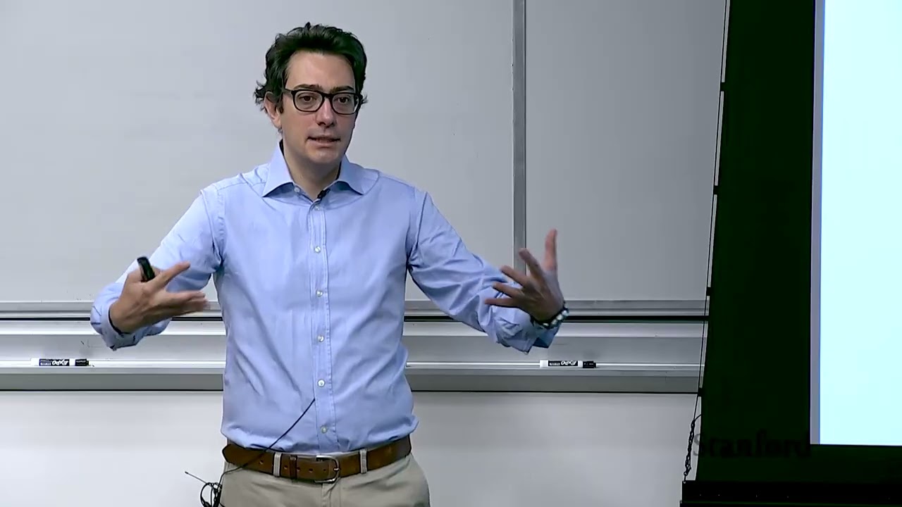
Pavone Derives Bayes Filter to Anchor Autonomous Robot Localization
Stanford Online
Control actions inherently disperse positional certainty while sensor observations contract it, requiring autonomous systems to resolve the tension through recursive Bayesian filtering.
Bayesian filtering provides the foundational probabilistic architecture for robotic state estimation, sequentially updating a robot's belief over its pose and environment as controls and noisy measurements arrive. (2:03)
Robotic state evolution exhibits an inherent asymmetry in knowledge: control actions induce uncertainty due to model mismatch and actuation noise, whereas sensor measurements reduce uncertainty by constraining feasible states. (45:54)
The continuous Bayes filter formalizes localization into a recursive two-step loop—predicting the state distribution via kinematics marginalization, then correcting it through Bayes' rule using sensor likelihoods. (58:28)
Because the raw continuous Bayes filter is computationally intractable in real time, practical autonomy relies on parametric approximations like Kalman filters or sample-based representations like particle filters. (53:31)
Detailed notes
## Background
This lecture was published on YouTube by Stanford Online on October 19, 2026, as part of the Stanford AA274A Principles of Robotic Autonomy course (Autumn 2019 edition). Delivered by Professor Marco Pavone, the video serves as Lecture 14 and introduces the mathematical theory of robot localization, probability foundations, and Bayesian filtering.
## TL;DR
Professor Marco Pavone opens the module on localization and mapping by contrasting reactive behavioral strategies with map-based state estimation. He provides a rigorous probability refresher covering random variables, conditional probability, total probability, and Bayes' rule, grounding these concepts in geometric intuition and the sample space. Pavone then models robot-environment interaction as a Hidden Markov Model, highlighting the tension between uncertainty-increasing control actions and uncertainty-reducing measurements. Finally, he derives the complete recursive Bayes filter, breaking down its prediction and measurement update steps as the computational blueprint for algorithms like Kalman and particle filters.
## Atmosphere & style
The lecture has an engaging, intellectually rigorous, and accessible academic atmosphere. Professor Pavone teaches with charismatic energy, frequently using geometric sketches, intuitive analogies, and candid humor to demystify dense probabilistic notation. His delivery combines high-stakes engineering realism—stressing that localization is vital for autonomy—with supportive, interactive checks for student understanding that keep the theoretical derivations grounded.
## Bulletin
- [02:03](https://www.youtube.com/watch?v=dG3-D-vDwe8&t=123s) Bayesian filtering provides the foundational probabilistic architecture for robotic state estimation, sequentially updating a robot's belief over its pose and environment as controls and noisy measurements arrive.
- [45:54](https://www.youtube.com/watch?v=dG3-D-vDwe8&t=2754s) Robotic state evolution exhibits an inherent asymmetry in knowledge: control actions induce uncertainty due to model mismatch and actuation noise, whereas sensor measurements reduce uncertainty by constraining feasible states.
- [58:28](https://www.youtube.com/watch?v=dG3-D-vDwe8&t=3508s) The continuous Bayes filter formalizes localization into a recursive two-step loop—predicting the state distribution via kinematics marginalization, then correcting it through Bayes' rule using sensor likelihoods.
- [53:31](https://www.youtube.com/watch?v=dG3-D-vDwe8&t=3211s) Because the raw continuous Bayes filter is computationally intractable in real time, practical autonomy relies on parametric approximations like Kalman filters or sample-based representations like particle filters.
## Key takeaways
- [00:05](https://www.youtube.com/watch?v=dG3-D-vDwe8&t=5s) The autonomous stack integrates four distinct modules: perception, localization and mapping, decision-making, and trajectory optimization/control.
- [03:19](https://www.youtube.com/watch?v=dG3-D-vDwe8&t=199s) Behavioral localization relies on reactive rules without an explicit map, whereas map-based localization tracks poses relative to an internal spatial model and generalizes across diverse environments.
- [06:59](https://www.youtube.com/watch?v=dG3-D-vDwe8&t=419s) Belief distributions quantify uncertainty over state space, balancing expressiveness against computational complexity across unimodal, multimodal, discrete, and continuous representations.
- [12:11](https://www.youtube.com/watch?v=dG3-D-vDwe8&t=731s) In continuous probability, the probability of any single exact coordinate is mathematically zero, necessitating probability density functions integrated over intervals.
- [15:29](https://www.youtube.com/watch?v=dG3-D-vDwe8&t=929s) Conditional probability formalizes the renormalization of the sample space to an observed event, establishing the fundamental operational tool for probabilistic state updates.
- [27:38](https://www.youtube.com/watch?v=dG3-D-vDwe8&t=1658s) Bayes' rule mathematically inverts forward sensor models into state posterior probabilities conditioned on observed sensor data.
- [32:05](https://www.youtube.com/watch?v=dG3-D-vDwe8&t=1925s) The denominator in Bayes' rule acts as a normalization constant that is constant across state hypotheses for a given measurement update cycle.
- [36:20](https://www.youtube.com/watch?v=dG3-D-vDwe8&t=2180s) Absolute independence and conditional independence do not imply each other; adding or removing conditioning variables can introduce or destroy statistical dependencies.
- [39:10](https://www.youtube.com/watch?v=dG3-D-vDwe8&t=2350s) Expectation serves as a linear operator providing the first moment of a distribution, while covariance measures joint linear variability between random variables.
- [49:31](https://www.youtube.com/watch?v=dG3-D-vDwe8&t=2971s) A state satisfies the Markov property when past state and measurement histories provide no additional predictive information once the current state is known.
- [51:58](https://www.youtube.com/watch?v=dG3-D-vDwe8&t=3118s) The measurement model depends solely on the current state, meaning sensor reading likelihoods are conditionally independent of previous trajectory histories.
- [53:31](https://www.youtube.com/watch?v=dG3-D-vDwe8&t=3211s) State estimation treats physical localization as a Hidden Markov Model, where true states remain unobservable and must be inferred from controls and measurements.
- [01:05:08](https://www.youtube.com/watch?v=dG3-D-vDwe8&t=3908s) The measurement update step scales the predicted belief by the likelihood of observing the current sensor measurement given each state candidate.
- [01:10:59](https://www.youtube.com/watch?v=dG3-D-vDwe8&t=4259s) The prediction step marginalizes over all prior state hypotheses by convolving the previous posterior belief with the kinematic transition probability model.
- [01:13:57](https://www.youtube.com/watch?v=dG3-D-vDwe8&t=4437s) Under output feedback control policies, the current control input can be dropped from the conditioning of the prior belief because it contains no new information beyond previous measurements.
## Detailed walkthrough
### [00:05](https://www.youtube.com/watch?v=dG3-D-vDwe8&t=5s) The Autonomous Stack and Localization
Professor Marco Pavone opens the third major part of the course, which focuses on robot localization and mapping. Returning to the foundational "see, think, act" paradigm introduced in Lecture 1, Pavone reviews the four-module architecture common to autonomous vehicle stacks:
1. **Perception**: Takes in sensor data and performs preprocessing such as filtering, object detection, and motion primitive extraction.
2. **Localization and Mapping**: Fuses perception output with a priori information to determine the robot's pose in the world and its spatial relationship to surrounding objects.
3. **Decision-Making**: Ingests the scene understanding to make high-level behavioral choices, such as lane changes or velocity adjustments.
4. **Trajectory Optimization and Control**: Translates behavioral decisions into low-level actuator commands.
Having addressed trajectory optimization and control in Module 1 and perception over the preceding two weeks, the course now moves to localization and mapping.
```mermaid
flowchart LR
accTitle: Autonomous System Stack Architecture
accDescr: Four-stage pipeline from perception to actuation
subgraph Sense ["See"]
P["Perception Module"]
end
subgraph Plan ["Think"]
LM["Localization & Mapping"]
DM["Decision-Making"]
end
subgraph Act ["Act"]
TC["Trajectory Optimization & Control"]
end
P --> LM
LM --> DM
DM --> TC
```
[02:03](https://www.youtube.com/watch?v=dG3-D-vDwe8&t=123s) Probability Theory and Bayesian Filtering
Pavone emphasizes that probability theory serves as the mathematical foundation of localization and mapping. Although probability theory is a formal prerequisite for the course, Pavone provides a concise refresher of key theoretical results before using them to derive the cornerstone of robotic state estimation: Bayesian filtering. Bayesian filtering formalizes how a robot sequentially refines its belief over uncertain quantities—specifically its pose and environment map—by incorporating sensor measurements over time. All subsequent discussions over the next three to four lectures build directly on this Bayesian framework.
Highlighting the necessity of localization, Pavone states: “If you don't know where you are and if you don't know where the objects are with respect to you, you can be as clever as you want, but you can be neither safe nor efficient.”
[03:19](https://www.youtube.com/watch?v=dG3-D-vDwe8&t=199s) Behavioral vs. Map-Based Localization
Pavone contrasts two fundamentally different and largely orthogonal paradigms for localization: the behavioral approach and the map-based approach.
In the **behavioral approach**, an engineer designs a set of reactive behaviors that jointly produce the desired motion. A canonical example is a simple wall-following rule: keeping a wall on the robot's right-hand side, which can successfully guide an agent to explore an entire room. Pavone explains why this approach is appealing: “Well, one of the key reasons is that it avoids to explicit reason about localization and mapping. You don't need to build a map in order to perform such a behavior and you don't need to localize yourself with respect to the map.” The behavioral strategy offers computational simplicity, bio-inspiration, and robust execution with minimal assumptions. However, it fails to scale to arbitrary, complex environments.
The **map-based approach**, which forms the primary focus of this class, maintains an explicit estimate of the robot's pose relative to an internal spatial map:
- The map can either be precomputed beforehand (standard practice in commercial self-driving cars, as highlighted in week 1's keynote) or constructed concurrently with pose estimation via Simultaneous Localization and Mapping (SLAM).
- While map-based systems are mathematically intricate, computationally heavy, and brittle when internal state estimates diverge from physical reality (such as estimating a position 3 meters away from ground truth), they generalize across arbitrary environments provided distinguishable landmarks exist.
[06:59](https://www.youtube.com/watch?v=dG3-D-vDwe8&t=419s) Belief Representations: Continuous, Discrete, Unimodal, and Multimodal
In map-based localization, systems must resolve two primary design questions:
1. **Map Representation**: The choice between fine-grained metric models (such as finely discretized 3D grids) and topological models that encode connectivity between high-level features (such as tables or walls) without explicit geometry.
2. **Belief Representation**: How the system represents its positional confidence over the map.
Belief is formalized as a probability distribution that simultaneously encodes the estimated position and the associated uncertainty. System designers face two critical modeling trade-offs when selecting a belief representation:
- **Unimodal vs. Multimodal Beliefs**: A unimodal belief assumes a single mode or peak (such as a Gaussian distribution, where the filter repeatedly projects state estimates onto a normal curve). Multimodal distributions allow multiple probability peaks across distinct areas of the environment. Pavone notes that multimodal representations are more realistic: “So, if I magically drop you in a room at Stanford, you might have an idea that maybe you are in an NVIDIA auditorium or maybe you are in another auditorium. Those would be the two peaks.” Despite this advantage, unimodal models are computationally tractable and function well when tracking local motion along an expected trajectory. Pavone reflects: “Everything in engineering is a compromise between how much powerful you want to be in your representations and how effective that is.”
- **Continuous vs. Discrete Representations**: Designers must decide whether coordinates should be treated continuously in real space or discretized into specific state intervals.
[10:49](https://www.youtube.com/watch?v=dG3-D-vDwe8&t=649s) Belief Representations and the Foundation of Bayesian Filtering
To represent robot location under uncertainty, one can either maintain a continuous probability distribution over every point in the environment or use a discretized representation yielding a histogram. In a one-dimensional example, the horizontal axis represents distance and the vertical axis represents the probability or percentage likelihood that the robot is at that specific location. The central challenge in probabilistic localization is determining how to update this belief when new measurements arrive. Prof. Marco Pavone identifies the primary method: "And the key tool we will be exploiting is the tool of Bayesian filtering."
Because Bayesian filtering is inherently probabilistic, all physical quantities involved in localization and mapping—such as robot state, control inputs, and sensor streams—are treated as random variables. Pavone points out the linguistic irony: “As you know, the name random variable is a bit of a misnomer because a random variable is technically a function, so it's not a random or variable.” Rather, it is a deterministic mathematical function mapping outcomes from an unpredictable sample space into real numbers.
```mermaid
flowchart TD
accTitle: Bayesian Belief Update Pipeline
accDescr: Diagram showing how continuous or discrete states are updated via measurements into a posterior belief using Bayesian filtering.
subgraph FilterEngine["Bayesian Filtering"]
BF["Bayes Filter Update"]
end
CRV --> BF
DRV --> BF
Z --> BF
U --> BF
BF --> Posterior["Updated Belief: bel(x_t)"]
```
---
[12:11](https://www.youtube.com/watch?v=dG3-D-vDwe8&t=731s) Review of Discrete and Continuous Random Variables
Pavone reviews the mathematical mechanics of discrete versus continuous random variables. Discrete random variables are characterized by a probability mass function (PMF). Using capital letters for random variables and lowercase letters for their realizations, the PMF assigns the probability that a random variable $X$ takes the specific value $x$, written as $P(X = x)$. For brevity, this is often written simply as $P(x)$, which represents a known value given by a system designer or estimated empirically from data. In adherence to probability axioms, the PMF must be normalized:
$$\sum_x P(X = x) = 1$$
For continuous random variables, the mechanics shift from summations to integrals, a change that introduces deeper mathematical nuances such as Lebesgue integration in advanced theory. Crucially, the probability that a continuous random variable takes on any single exact value $x$ is zero ($P(X = x) = 0$), because there is an uncountably infinite continuum of outcomes. Pavone clarifies: “Remember, the probability zero doesn't mean impossible. Just mean probability zero.” Instead, meaningful probabilities are defined over intervals $[a, b]$ using a probability density function (PDF), $p(x)$:
$$P(a \le X \le b) = \int_a^b p(x)\,dx$$
Here, $p(x)\,dx$ represents the probability that the random variable falls within an infinitesimal interval $[x, x + dx]$. Like PMFs, continuous PDFs must integrate to 1 over the entire support of the random variable:
$$\int_{-\infty}^{\infty} p(x)\,dx = 1$$
- Capital letters (e.g., $X, Y$) denote random variables; lowercase letters (e.g., $x, y$) denote specific values or realizations.
- $P(x)$ serves as shorthand notation for $P(X = x)$.
- Continuous density functions must satisfy normalization over their full domain: $\int p(x)\,dx = 1$.
---
[15:29](https://www.youtube.com/watch?v=dG3-D-vDwe8&t=929s) Joint Distributions, Independence, and the Definition of Conditional Probability
Robotics requires tracking several quantities at once—robot state, sensor readings, and commanded controls. Consequently, localization relies on joint distributions over multiple random variables. For two random variables $X$ and $Y$, the joint probability is defined as $P(x, y) = P(X = x \text{ and } Y = y)$. A central property is independence: two variables are independent if their joint distribution factors cleanly into the product of their marginals ($P(x, y) = P(x)P(y)$).
To clarify why this factorization makes intuitive sense, Pavone transitions to conditional probability, which alongside Bayes' theorem forms the bedrock of Bayesian filtering. When observing an outcome $Y = y$ that carries information about $X$, the conditional probability of $X$ given $Y$ (assuming $P(y) > 0$) is defined by:
$$P(x \mid y) = \frac{P(x, y)}{P(y)}$$
Pavone emphasizes the epistemic status of this formula: “First of all, what is important to notice is that this is not a theoretical result. So, this is not something that we derived from other results. This is indeed definition.” In many mathematical formulations, this relation serves directly as an axiom. It formalizes the process of renormalizing the joint event space by the probability of an observed condition.
---
[18:34](https://www.youtube.com/watch?v=dG3-D-vDwe8&t=1114s) Geometric Intuition: The Sample Space (Omega Space)
To prevent confusion about conditional probability, Pavone advises students to ground their reasoning geometrically in the sample space (the $\Omega$ space of possible outcomes). He illustrates this using a unit rectangle of total area 1, onto which a point is thrown at random with uniform distribution, meaning the probability of hitting any set equals its geometric area. He sketches three subsets:
- Set $A$ with area $0.75$ ($P(A) = 0.75$)
- Set $B$ with area $0.5$ ($P(B) = 0.5$)
- Set $C$ with area $0.25$, lying entirely within $A$
Pavone asks the class to calculate $P(A \mid B)$ given that the overlap between $A$ and $B$ (the intersection $A \cap B$) has an area of $0.25$. When a student initially guesses 25%, another corrects it to 50%. Pavone steps through the reasoning: knowing that the event is restricted to $B$ rescales the universe to $B$'s area ($0.5$). The conditional probability is the ratio of the intersection area to the new restricted domain:
He then asks for $P(A \mid C)$, knowing that $C$ has an area of $0.25$ and lies completely inside $A$. The overlap is $0.25$, yielding $0.25 / 0.25 = 1.0$ (100%). Emphasizing how quickly intuition can fail when manipulating raw formulas without visualization, Pavone delivers a rule of thumb for probability calculations: “Always go back to the sample space if you have any confusion. Trust me. It's the only way to clear any confusion.”
| Set / Event | Area / Prior Probability | Overlap with $A$ ($A \cap \text{Set}$) | Conditional Probability Given Set |
|:--- |:--- |:--- |:--- |
| **Set $A$** | $P(A) = 0.75$ | $0.75$ | $P(A \mid A) = 1.0$ ($100\%$) |
| **Set $B$** | $P(B) = 0.50$ | $0.25$ | $P(A \mid B) = \frac{0.25}{0.50} = 0.50$ ($50\%$) |
| **Set $C$** | $P(C) = 0.25$ | $0.25$ | $P(A \mid C) = \frac{0.25}{0.25} = 1.0$ ($100\%$) |
[24:09](https://www.youtube.com/watch?v=dG3-D-vDwe8&t=1449s) Independence and the Law of Total Probability
Building directly on the definition of conditional probability, Prof. Marco Pavone shows why statistical independence is defined the way it is. If two random variables $X$ and $Y$ are independent, their joint distribution factors cleanly as $P(X, Y) = P(X)P(Y)$. Plugging this into the conditional probability formula yields:
As Pavone summarizes, “For two independent random variables, the probability of $X$ given $Y$ is simply given equal to the unconditional probability, which basically means that $Y$ does not carry over any information about $X$.” Together with Bayes' theorem, these foundational concepts form the core toolkit needed for the course.
Pavone then introduces the law of total probability, describing it as a convenient computational trick derived from the axioms of probability regarding non-overlapping events. If the unconditional distribution $P(X)$ is unknown, but the joint distribution with another variable $Y$ is accessible, $P(X)$ can be recovered by marginalizing over all possible realizations of $Y$:
For continuous random variables, the summations are replaced with integrals, and probability mass functions become probability density functions. Pavone points out that while formal proofs exist and take only a couple of lines on Wikipedia, the mechanical application is what matters for filtering.
Pavone transitions to Bayes' rule, emphasizing that it allows one to invert probabilistic conditioning between random variables $X$ and $Y$. In robotics, this inversion is essential. Letting $Y$ represent observed sensor data (such as a lidar range scan) and $X$ denote an unobserved state (such as the robot's spatial coordinate), the engineer typically needs $P(X \mid Y)$—the probability of being at location $X$ given the measurement $Y$. However, forward physical models and sensor characterization naturally yield $P(Y \mid X)$ instead—answering questions such as: if the robot is located at $X$, what is the probability of reading a lidar distance of 30 cm?
Bayes' rule bridges this gap through two direct applications of conditional probability combined with the law of total probability:
1. By conditional probability: $P(X \mid Y) = \frac{P(X, Y)}{P(Y)}$
2. Conditioning in reverse: $P(X, Y) = P(Y \mid X)P(X)$
3. Substituting the numerator: $P(X \mid Y) = \frac{P(Y \mid X)P(X)}{P(Y)}$
4. Expanding the denominator via total probability: $P(Y) = \sum_{X'} P(Y \mid X')P(X')$
Pavone notes that he deliberately writes $X'$ in the denominator summation to distinguish the specific hypothesis $X$ being evaluated from the dummy integration/summation variable $X'$ iterating over all possible locations.
```mermaid
flowchart LR
accTitle: Bayesian Inference Flow
accDescr: Diagram illustrating how prior beliefs and sensor likelihood combine to form posterior beliefs over state.
[32:05](https://www.youtube.com/watch?v=dG3-D-vDwe8&t=1925s) Bayesian Filtering and the Normalization Constant ($\eta$)
Pavone highlights the practical philosophy of the course: “This is interesting result in its own right, but in this class, we are opportunistic, and we only care about theoretical results if they allow us to do stuff.” In robotics, Bayes' rule powers Bayesian filtering, allowing an autonomous agent to fuse prior beliefs with noisy incoming observations to update its state estimate over time. Underscoring the centrality of this relation, Pavone warns the room: “If you understand this, the next five lectures will be pretty straightforward. If you don't understand this, the next five lectures will be hell.”
To streamline implementation and avoid redundant math, the denominator $P(Y)$ is often replaced by a normalization constant $\eta$:
Because the denominator sums over all candidate states $X'$, it does not vary when evaluating different values of $X$ against the same measurement data $Y$. Pavone reminds students that it would be computationally wasteful to re-evaluate the denominator from scratch when checking the likelihood of $X = 2$ versus $X = 3$.
When a student asks whether $\eta$ must be recomputed as new data arrives, Pavone clarifies immediately:
- $\eta$ is constant with respect to the state hypothesis $X$ for a fixed measurement $Y$, so it only needs to be computed once per measurement update cycle.
- Once fresh sensor data $Y$ arrives in subsequent iterations, the denominator depends on the new data and must indeed be recalculated for that new time step.
[36:20](https://www.youtube.com/watch?v=dG3-D-vDwe8&t=2180s) Extending Probability Definitions to Conditioning on Arbitrary Variables
Prof. Marco Pavone wraps up the foundational probability review before transitioning to the localization problem, explaining that all prior results regarding conditional probabilities and independence extend naturally when conditioning on an arbitrary random variable $Z$. Using Bayes' rule as a primary example, if an additional random variable $Z$ takes on the value $z$, the probability of $X$ given $Y$ and $Z$ is formulated by consistently carrying the conditioning:
Similarly, two random variables $X$ and $Y$ are conditionally independent given $Z$ if their conditional probability distribution factors with respect to $Z$:
$$P(X, Y \mid Z) = P(X \mid Z) \, P(Y \mid Z)$$
Adding conditioning variables preserves the core mathematical structures intact.
```mermaid
flowchart TD
accTitle: Independence vs Conditional Independence
accDescr: Diagram illustrating that absolute independence and conditional independence do not imply one another.
subgraph IndependenceRelations["Independence Relationships"]
Indep["Absolute Independence:<br/>P(X, Y) = P(X)P(Y)"]
CondIndep["Conditional Independence:<br/>P(X, Y | Z) = P(X | Z)P(Y | Z)"]
end
Indep -- "Does NOT imply" --> CondIndep
CondIndep -- "Does NOT imply" --> Indep
```
Prof. Pavone cautions against a common point of confusion: conditional independence does not imply absolute (unconditional) independence, nor does absolute independence imply conditional independence. Two random variables can be conditionally independent given $Z$ yet dependent once the conditioning is removed. Conversely, two unconditionally independent variables can become dependent when conditioning on $Z$, “simply because that $Z$ may carry over some information that relates $X$ and $Y$.” He reminds the class that counterexamples are easy to construct and promises an explicit robotics-related example later in the lecture.
[39:10](https://www.youtube.com/watch?v=dG3-D-vDwe8&t=2350s) Succinct Representations of Distributions: Expectation and Covariance
While a full probability distribution function completely describes a random variable, it is often a high-dimensional, computationally intractable object to manipulate in practice. To summarize distributions concisely, roboticists rely on representative numbers, chief among them the expectation (mean) and covariance. The expectation is defined discretely as the sum of all possible values weighted by their probabilities:
$$E[X] = \sum x \cdot P(X = x)$$
For continuous distributions, this summation becomes an integral. Prof. Pavone notes that expectation captures the intuition of the "most likely event" in a distribution.
A critical mathematical property is that expectation is a linear operator:
$$E[AX + B] = A \, E[X] + B$$
Prof. Pavone emphasizes the generality of this identity: “This is one of the very few results in probability theory that holds without any assumptions. Just by structurally exploiting the properties of additivity of the summation.” When dealing with a random vector, the expectation is taken component-wise.
The second essential summary metric is covariance, which quantifies the joint variability between two random variables $X$ and $Y$:
If perturbations in $X$ cause $Y$ to move in a completely random direction, their covariance is zero; if their variations align along a line, their normalized correlation coefficient reaches $1$ or $-1$.
[42:17](https://www.youtube.com/watch?v=dG3-D-vDwe8&t=2537s) Modeling Robot-Environment Interaction: States, Measurements, and Controls
Turning to the formulation of the localization problem, Prof. Pavone assumes for the next couple of lectures that a map of the environment is already known. The immediate goal is simply to determine where the robot is located within this given map, postponing the harder problem of simultaneous localization and mapping (SLAM) to future lectures.
At a high level, a robot interacts with its environment in two primary ways: it enacts control actions to alter the physical state, and it gathers perceptual measurements to obtain information. To mathematically formalize this loop, three fundamental components are defined:
```mermaid
flowchart LR
accTitle: Robot Interaction Loop
accDescr: Flow diagram showing how control inputs act on the state and how measurements are gathered from the state.
subgraph World["Environment & Robot"]
State["State x_t<br/>(Robot pose, orientation, objects)"]
end
subgraph Operations["Actions and Perceptions"]
Control["Control u_t<br/>(Induces loss of knowledge)"]
Measurement["Measurement z_t<br/>(Increases knowledge)"]
end
Control -->|"Drives transition"| State
State -->|"Generates observation"| Measurement
```
- **State ($x_t$):** The collection of all aspects of the robot and its environment at time $t$ that can impact the future, such as the robot's pose (position and orientation), velocity, and surrounding objects. State histories over a time interval $t_1$ to $t_2$ are compactly indexed as $x_{t_1:t_2}$.
- **Markov Property (State Completeness):** A state is complete if no historical state prior to $x_t$ provides additional predictive power regarding future states. Given $x_t$ and future control actions, the future state evolution is conditionally independent of past trajectory history: knowing $x_{0:t-1}$ yields no extra predictive information. This prediction remains stochastic rather than deterministic due to disturbances like wind gusts or wheel slip.
- **Measurements ($z_t$):** Sensor observations providing momentary snapshots of the environment, such as range readings from a lidar sensor. Sensor histories are denoted $z_{t_1:t_2}$.
- **Controls ($u_t$):** Commanded actions (such as wheel velocities or motor torques) that produce changes in the environmental state, with histories denoted $u_{t_1:t_2}$.
[45:54](https://www.youtube.com/watch?v=dG3-D-vDwe8&t=2754s) The Asymmetry of Knowledge: Measurement Updates vs. Control Actions
Prof. Pavone draws attention to an asymmetry that frequently confuses students regarding how uncertainty propagates through control actions versus measurement updates. Measurements constrain the set of possible robot configurations, thereby increasing knowledge and reducing uncertainty. In contrast, enacting control actions induces a loss of knowledge and increases uncertainty.
To explain why control actions disperse knowledge, Prof. Pavone prompts the class, and a student observes that real-world movement never executes perfectly. Prof. Pavone confirms:
> “So since once we enact the control action, we might have a disturbance, model mismatches, and number of stuff. As we move, say that we are here, actually we might end up here or we might end up here. And since I don't know exactly where I am, I have to apply the same process for all possible points that I could be, which means that basically this set is growing.”
Because of unmodeled dynamics, actuation noise, and environmental disturbances, moving from an already uncertain initial set causes the envelope of potential locations to dilate. This foundational tension—controls dispersing belief and measurements contracting it—forms the operational core of Bayesian filtering for robot localization.
[47:32](https://www.youtube.com/watch?v=dG3-D-vDwe8&t=2852s) The Ballet of Localization and State Transition Modeling
Localization functions fundamentally as a continuous tension between two opposing forces: control actions that inject noise and increase uncertainty, balanced by sensor measurements that provide information and decrease uncertainty. To capture how these ingredients evolve over time and derive the governing filtering equations, the system dynamics are represented using a probabilistic generative model. The state at time step $t$ is generated stochastically, described by a probability density function (or probability mass function in discrete spaces) conditioned on the history of states, measurements, and control inputs: $p(x_t \mid x_{0:t-1}, z_{1:t-1}, u_{1:t})$.
```mermaid
flowchart LR
accTitle: Sequence of State Events
accDescr: Sequence showing transition from prior state through measurement and control action to the next state.
subgraph StepTMinus1["Step t - 1"]
Xprev["State x(t-1)"]
end
subgraph StepT["Step t"]
Ucurr["Control u(t)"]
Xcurr["State x(t)"]
Zcurr["Measurement z(t)"]
end
Xprev --> Ucurr
Ucurr --> Xcurr
Xcurr --> Zcurr
```
Addressing potential confusion regarding the time index of the control input extending up to $t$ rather than $t-1$, Pavone emphasizes that this choice is an intentional convention rather than a clerical error: “So, why is this a typo? Am I sloppy that I didn't put $t - 1$ here? No.” The sequence of physical events follows an intuitive order: the robot enters state $x_t$, records a sensor measurement $z_t$, and applies a control input $u_t$ that carries it forward to the subsequent state. While alternative conventions can be structured, this ordering represents the most natural framework for modeling recursive robot state transitions.
[49:31](https://www.youtube.com/watch?v=dG3-D-vDwe8&t=2971s) The Completeness of State and the Markov Property
A foundational modeling assumption in robotic localization is state completeness—commonly referred to as the Markov property. Under this assumption, the past contains no predictive value beyond what is already captured in the immediate preceding state. Mathematically, conditional independence allows the state distribution conditioned on the entire history to collapse into a much simpler distribution conditioned solely on the previous state and the current control:
When asked by a student why state completeness might sometimes be a poor assumption, Pavone notes that although state vectors can theoretically be augmented to recover Markovian behavior, real-world interactions often violate simple state definitions:
> “So, when you're trying to change your lane, your action and your prediction about what the human will do in the future does not depend just on what the human is doing right now, but what it has done maybe for the past two or three seconds.”
If an observed driver has been driving recklessly over preceding seconds, that behavioral history drastically changes collision predictions in ways that instantaneous relative velocity and separation distance alone cannot reveal. While such non-Markovian interactions represent active frontiers of research in autonomous driving and human-robot interaction, the standard Markov property remains sufficient for foundational localization. When an audience member asks why conditional independence holds, Pavone explains that while past measurements help identify the earlier location $x_{t-1}$, once $x_{t-1}$ is known with certainty, those prior measurements provide no additional information about the transition into $x_t$.
[51:58](https://www.youtube.com/watch?v=dG3-D-vDwe8&t=3118s) Measurement Models and Hidden Markov Networks
The observation process mirrors the Markovian structure of the state transition model. Known as the measurement or sensor model, the probability distribution over the current measurement $z_t$ conditioned on the robot’s full trajectory history reduces directly to the measurement conditioned purely on the current state:
Pavone illustrates the physical intuition behind this formulation with a spatial example: “So the fact that the measured range equal to 30 m given that I'm position $x_t$, the probability of that measurement is exactly the same whether in the past I came from San Francisco or I came from San Jose.” Once the robot's physical coordinate is fixed, the mechanics of range sensing operate independently of how the robot traveled to reach that coordinate.
```mermaid
flowchart TD
accTitle: Dynamic Bayesian Network
accDescr: Hidden Markov model topology showing transitions between hidden states, actions, and observations.
subgraph HiddenLayer["Hidden States"]
Xtminus1["x(t-1)"]
Xt["x(t)"]
end
subgraph ObservedLayer["Observed Variables"]
Ut["Control u(t)"]
Ztminus1["Measurement z(t-1)"]
Zt["Measurement z(t)"]
end
Xtminus1 --> Xt
Xtminus1 --> Ztminus1
Ut --> Xt
Xt --> Zt
```
Viewed through the lens of dynamic Bayesian networks, this system forms a classic Hidden Markov Model (HMM). The states $x_t$ are hidden variables that cannot be observed directly. Instead, an autonomous agent interacts with the world solely through the controls $u_t$ it executes and the noisy observations $z_t$ it collects. The fundamental objective of localization is to deduce the distribution over these hidden state variables from the history of available controls and measurements.
[53:31](https://www.youtube.com/watch?v=dG3-D-vDwe8&t=3211s) Defining Beliefs and the Bayes Filter Architecture
Because the true state remains unobservable, the robot maintains a mathematical representation of its uncertainty known as a belief. A belief is a posterior probability distribution over state hypotheses given all sensor data and control inputs gathered up to the present moment:
For computational convenience, the filtering pipeline splits this estimation into two sequential stages by introducing the prediction belief (often written $\overline{\text{bel}}(x_t)$):
The prediction belief incorporates the most recent control input $u_t$ without yet factoring in the concurrent measurement $z_t$. Transitioning from $\overline{\text{bel}}(x_t)$ to the full belief $\text{bel}(x_t)$ constitutes the measurement update or correction step, which refines the state distribution using the latest sensory evidence.
This two-step process defines the Bayes filter, the cornerstone of map-based robotic localization and mapping:
- **Generality and Practical Limits**: The Bayes filter relies strictly on state completeness without imposing parametric restrictions (such as Gaussian distributions or linear kinematics), making it applicable to arbitrary measurement network models.
- **Computational Tractability**: In its raw, continuous, infinite-dimensional form, the Bayes filter cannot be computed directly on embedded hardware; subsequent lectures introduce parametric filters (like Kalman filters) and sample-based approximations (like particle filters) to make updates solvable.
- **Initial Prior ($\text{bel}(x_0)$)**: Iterative execution begins with a prior distribution. In the absence of prior positional information, the initial belief is initialized uniformly across the operating domain—such as spreading probability mass across the entire Stanford campus or across the surface of the Earth.
- **Recursive Execution**: At step $t$, the filter ingests the previous posterior $\text{bel}(x_{t-1})$, the applied control $u_t$, and the new observation $z_t$ to compute the updated posterior belief $\text{bel}(x_t)$.
[58:28](https://www.youtube.com/watch?v=dG3-D-vDwe8&t=3508s) The Two-Step Bayes Filter Architecture
```mermaid
flowchart TD
accTitle: Two-Step Bayes Filter Flow
accDescr: Diagram showing how belief at t-1 transitions to prediction belief via control u_t, and then to full belief via measurement z_t.
subgraph Prior ["Prior State"]
Bprev["Belief bel(x_{t-1})"]
end
subgraph Step1 ["Step 1: Prediction"]
Ut["Control u_t"]
Bbar["Prediction Belief \bar{bel}(x_t)"]
Bprev --> Bbar
Ut --> Bbar
end
Prof. Pavone introduces the central question of state estimation: given that a robot lacks direct access to its true state $x_t$, the best it can achieve within its modeling framework is to compute the probability distribution over all possible locations—the belief $\text{bel}(x_t)$. To do this, the algorithm operates in a two-step cycle for every possible state hypothesis $x_t$.
The cycle alternates between a motion update and a measurement update. First, starting from the prior distribution at time $t-1$, the algorithm accounts for the most recent control input $u_t$ to compute the prediction belief (often denoted $\overline{\text{bel}}(x_t)$). Second, it incorporates the most recent sensor measurement $z_t$ to produce the full posterior belief $\text{bel}(x_t) = p(x_t \mid z_{1:t}, u_{1:t})$. The algorithm then repeats this evaluation over all possible values of $x_t$.
- **Step 1 (Prediction / Time Update):** Refines the prior belief from time $t-1$ by folding in the latest control action $u_t$.
- **Step 2 (Correction / Measurement Update):** Adjusts that predicted probability by conditioning on the newly received observation $z_t$.
---
[59:44](https://www.youtube.com/watch?v=dG3-D-vDwe8&t=3584s) Intuition Behind the Prediction Step
Prof. Pavone breaks down the physical intuition of the prediction equation before diving into formal math. Suppose the robot possesses full knowledge of its belief distribution at time $t-1$. Because it cannot be certain of its exact prior position, it must evaluate an array of candidate hypotheses: $x_{t-1}^{(1)}, x_{t-1}^{(2)}, \dots, x_{t-1}^{(n)}$. For each hypothesis, the prior belief provides the relative likelihood that the robot was actually there.
From each of those potential prior states, applying the control command $u_t$ yields a transition probability $p(x_t \mid x_{t-1}, u_t)$ of arriving at the candidate state $x_t$. To evaluate the overall probability of ending up at $x_t$, the filter takes a weighted sum over every possible starting point, scaling the probability of each starting hypothesis by the likelihood of transitioning from it to $x_t$:
If the probability of transitioning from a given $x_{t-1}$ to $x_t$ under control $u_t$ is zero, that starting hypothesis contributes nothing to the outcome.
> “What is the probability that I’m here? Well, let’s look at where I could come here from all the possible places where I could be at the previous steps, and let’s account for what is the probability that from all those previous places, I can come to here. And then I sum all of them.” — Prof. Marco Pavone
---
[01:02:35](https://www.youtube.com/watch?v=dG3-D-vDwe8&t=3755s) Intuition Behind the Measurement Update and Normalization
Turning to the second step, Prof. Pavone explains how incoming sensor data modulates the predicted distribution. Even if the prediction step assigns a high probability (such as 0.7) to a state $x_t$, the filter must cross-reference that hypothesis against the observed sensor measurement $z_t$. If the likelihood of observing a range reading of $0.3\text{ m}$ from that candidate state is zero, the posterior probability of being at that state drops immediately to zero.
The measurement update effectively amplifies or demodulates the predicted probabilities based on how compatible each state hypothesis is with the sensor reading. Because this update relies on Bayes' rule, it introduces the normalizing constant $\eta$ (or $\eta^{-1}$ in the denominator), which does not depend on the specific state $x_t$ being evaluated. In practice, an implementation computes the unnormalized values across the state space, sums or integrates them, and divides by the total so the resulting distribution integrates to 1.
Prof. Pavone emphasizes that this conceptual blueprint underlies the rest of the localization curriculum:
> “The reason why I’m spending so much time here is that everything else we’re going to do is basically a refinement of this fundamental algorithm to make it computable, to something that you can code.” — Prof. Marco Pavone
He notes that in Homework 4, students will implement an Extended Kalman Filter (EKF), which realizes this exact Bayes filter under the assumption that the underlying belief distribution is Gaussian.
---
[01:05:08](https://www.youtube.com/watch?v=dG3-D-vDwe8&t=3908s) Derivation of the Measurement Update via Bayes' Rule
```mermaid
flowchart LR
accTitle: Bayes Rule Expansion for Measurement Update
accDescr: Step-by-step mathematical expansion applying Bayes rule and the Markov property to derive the measurement update.
Prof. Pavone decides to derive the second step first, noting that it is a direct and elegant application of Bayes' rule. He reviews standard Bayes' theorem:
To apply this to the belief definition $\text{bel}(x_t) = p(x_t \mid z_{1:t}, u_{1:t})$, he designates $x_t$ as $X$ and the latest measurement $z_t$ as $Y$, treating all prior measurements $z_{1:t-1}$ and all control inputs $u_{1:t}$ as background conditioning variables that are carried throughout the derivation:
The denominator $p(z_t \mid z_{1:t-1}, u_{1:t})$ does not depend on $x_t$ and is absorbed into the normalizer $\eta$. The remaining terms simplify through two key insights:
1. **The Markov Property:** By the conditional independence assumption of the Markov model, once the true current state $x_t$ is known, past observations and controls provide no extra information about the current measurement $z_t$. Therefore:
$$p(z_t \mid x_t, z_{1:t-1}, u_{1:t}) = p(z_t \mid x_t)$$
2. **The Prediction Belief:** By definition, the term conditioning $x_t$ on $z_{1:t-1}$ and $u_{1:t}$ is the predicted belief $\overline{\text{bel}}(x_t)$, which accounts for the most recent control input but not yet the latest measurement.
Thus, the posterior belief relates to the prediction belief through a simple multiplicative sensor model factor:
- **Conditional Independence:** Past history carries no predictive power for $z_t$ once $x_t$ is fixed. As Prof. Pavone notes, “Usually, this is a good assumption, so this works.”
- **Measurement Model:** $p(z_t \mid x_t)$ is treated as a known likelihood function derived from sensor physics.
[01:09:45](https://www.youtube.com/watch?v=dG3-D-vDwe8&t=4185s) Recapping Step Two and Framing the Prediction Step
Prof. Marco Pavone wraps up the discussion of Step 2 (the measurement update) of the Bayes filter before turning to the first step. In Step 2, the sensor model characterizes the probability of observing a particular measurement given the robot's current state, allowing the algorithm to predict sensor readings conditioned on location. This measurement update relies on the predicted belief $\overline{\operatorname{bel}}(x_t)$, which is generated recursively in Step 1, alongside the normalizer $\eta$.
Turning to Step 1 (the prediction step), Pavone acknowledges that the derivation might look “slightly more involved, but not really.” The goal is to express the predicted belief $\overline{\operatorname{bel}}(x_t) = p(x_t \mid z_{1:t-1}, u_{1:t})$ purely in terms of known quantities: the prior belief from the previous step $\operatorname{bel}(x_{t-1})$, the state transition model $p(x_t \mid x_{t-1}, u_t)$, and the control inputs. The measurement model does not play any role in this first step.
```mermaid
flowchart LR
accTitle: Two-step Bayes Filter Cycle
accDescr: Diagram showing how belief at t minus 1 transitions through prediction step 1 to predicted belief, then through update step 2 to final belief at time t.
subgraph Step1["Step 1: Prediction"]
Bprev["bel(x_{t-1})"] --> Pred["Integrate over x_{t-1}<br/>using p(x_t | x_{t-1}, u_t)"]
Pred --> BelBar["bel̄(x_t)"]
end
subgraph Step2["Step 2: Measurement Update"]
BelBar --> Upd["Multiply by p(z_t | x_t)<br/>and normalize by η"]
Upd --> Bcurr["bel(x_t)"]
end
```
[01:10:59](https://www.youtube.com/watch?v=dG3-D-vDwe8&t=4259s) Applying Total Probability and the Markov Property to State Propagation
To make the computation tractable and connect it to known distributions, Pavone uses the law of total probability (marginalization) by introducing conditioning on $x_{t-1}$. In intuition terms: “We relate it to what we already know.” The robot knows its transition dynamics $p(x_t \mid x_{t-1}, u_t)$, so introducing $x_{t-1}$ bridges the unknown future state to the previous state. Because the state space is continuous, the marginalization takes the form of an integral over $x_{t-1}$:
Pavone breaks down the standard probability rule to reassure students that beneath the messy notation, the underlying operation is elementary: $p(x) = \sum_y p(x, y) = \sum_y p(x \mid y) p(y)$. Here, the added clutter comes entirely from the history of measurements and controls being carried along in the conditioning.
Next, the Markov assumption simplifies the first factor inside the integral: $p(x_t \mid x_{t-1}, z_{1:t-1}, u_{1:t})$ reduces to $p(x_t \mid x_{t-1}, u_t)$. Pavone notes: “Knowing the previous state $t$ minus one and the current control is all we need in order to estimate the $x$ of $t$. That's a Markov property again.” Just as the Markov property was applied to measurement independence in Step 2, it is now applied to state propagation. This factor represents the state transition model, analogous to the kinematic vehicle models from the first lecture, but treated probabilistically rather than deterministically.
- Known prior belief: $\operatorname{bel}(x_{t-1}) = p(x_{t-1} \mid z_{1:t-1}, u_{1:t-1})$.
- State transition model: $p(x_t \mid x_{t-1}, u_t)$ derived from the robot's kinematics under control input $u_t$.
- Prediction integral: $\overline{\operatorname{bel}}(x_t) = \int p(x_t \mid x_{t-1}, u_t) \, p(x_{t-1} \mid z_{1:t-1}, u_{1:t}) \, dx_{t-1}$.
[01:13:57](https://www.youtube.com/watch?v=dG3-D-vDwe8&t=4437s) Dropping the Current Control from the Prior Belief
The final step in the derivation involves the second factor in the integral: $p(x_{t-1} \mid z_{1:t-1}, u_{1:t})$. Pavone points out that this term is conditioned on all controls up to time $t$, including $u_t$. He argues that $u_t$ can be safely dropped from the conditioning set, making the term equal to $p(x_{t-1} \mid z_{1:t-1}, u_{1:t-1})$, which by definition is $\operatorname{bel}(x_{t-1})$.
```mermaid
flowchart LR
accTitle: Dynamic Bayesian Network Slice
accDescr: Visual depiction of state and measurement dependencies over time slices t-1 and t.
subgraph SlicePrev["Time t-1"]
Utminus1["u_{t-1}"] --> Xtminus1["x_{t-1}"]
Xtminus1 --> Ztminus1["z_{t-1}"]
end
subgraph SliceCurr["Time t"]
Ztminus1 -.->|"Feedback Policy"| Ut["u_t"]
Xtminus1 --> Xt["x_t"]
Ut --> Xt
end
```
To explain why this holds, Pavone draws a Dynamic Bayesian Network slice showing $u_{t-1} \to x_{t-1} \to z_{t-1}$, followed by the choice of new control $u_t$, which along with $x_{t-1}$ dictates $x_t$. If one is trying to estimate the past state $x_{t-1}$, knowing the future action $u_t$ adds no new information about where the robot already was:
> “So the fact that I tell you the control that we will apply in order to transition to $x_t$, what possibly information can carry in order to better estimate $x_{t-1}$?”
Under standard output feedback policies, the control $u_t$ is computed strictly as a function of past measurements (principally $z_{t-1}$ and prior observations). Because the expression is already conditioned on all those measurements $z_{1:t-1}$, the control $u_t$ is merely a compressed function of information already in the conditioning set: “It will just be a more compressed version of all the previous measurements, but it doesn't carry over any additional information.”
With $u_t$ dropped, $p(x_{t-1} \mid z_{1:t-1}, u_{1:t-1})$ evaluates to $\operatorname{bel}(x_{t-1})$, completing the prediction formula:
Pavone concludes the lecture by previewing the upcoming class: having derived the foundational mathematics and intuition behind the Bayes filter, the next step is making it computationally feasible. Real-time implementation requires approximations (such as Kalman filters or particle filters) to allow a robot to localize itself with respect to a map.
## Notable quotes
> [02:03](https://www.youtube.com/watch?v=dG3-D-vDwe8&t=123s) If you don't know where you are and if you don't know where the objects are with respect to you, you can be as clever as you want, but you can be neither safe nor efficient. — Prof. Marco Pavone
> [06:59](https://www.youtube.com/watch?v=dG3-D-vDwe8&t=419s) Everything in engineering is a compromise between how much powerful you want to be in your representations and how effective that is. — Prof. Marco Pavone
> [18:34](https://www.youtube.com/watch?v=dG3-D-vDwe8&t=1114s) Always go back to the sample space if you have any confusion. Trust me. It's the only way to clear any confusion. — Prof. Marco Pavone
## Mentioned
Marco Pavone, Stanford University, NVIDIA, NASA Jet Propulsion Laboratory, Massachusetts Institute of Technology, Barack Obama, Extended Kalman Filter, Principles of Robot Autonomy, Wikipedia
## Video description
For more information about Stanford’s graduate programs, visit: https://online.stanford.edu/graduate-education
Lecture 14 — Introduction to Localization and Filtering Theory
Note: This lecture was recorded as part of the 2019 edition of the course. Course content, structure, assignments, and other materials may have changed since this recording. The course links below point to the most recent edition and may therefore differ from what is presented in the video.
Read the companion textbook, Principles of Robot Autonomy, free online: https://porabook.com
Follow along with the latest course schedule and syllabus: https://stanfordasl.github.io/PoRA-I
Speaker: Prof. Marco Pavone
Dr. Marco Pavone is an Associate Professor of Aeronautics and Astronautics at Stanford University and a Senior Director of Autonomous Vehicle Research at NVIDIA. Prior to joining Stanford, he was a Research Technologist in the Robotics Section at NASA’s Jet Propulsion Laboratory. Dr. Pavone received his Ph.D. in Aeronautics and Astronautics from the Massachusetts Institute of Technology in 2010. His research focuses on the analysis, design, and control of autonomous systems, with particular emphasis on self-driving cars, autonomous aerospace vehicles, and future mobility systems. He has been recognized with numerous awards, including the Presidential Early Career Award for Scientists and Engineers from President Barack Obama, the Office of Naval Research Young Investigator Award, the NSF CAREER Award, the NASA Early Career Faculty Award, the IEEE Kiyo Tomiyasu Award, the CSS Award for Technical Excellence in Aerospace Control, and the Early-Career Spotlight Award from the Robotics Science and Systems Foundation.
Full playlist: https://www.youtube.com/playlist?list=PLR9iNyexfIkk
Professor Marco Pavone frames robotic localization as a recursive Bayesian state estimation problem within the autonomous stack, where an agent tracks its pose on a known map by resolving the mathematical tension between uncertainty-inducing control actions and information-providing sensor observations.
Map-Based Localization and Belief Representations (3:19)
Pavone distinguishes between behavioral localization, which relies on simple reactive heuristics like wall-following without explicit maps, and map-based localization, which maintains an explicit state estimate relative to an internal spatial representation. While behavioral approaches are computationally lightweight, they fail to scale across complex environments. Map-based localization generalizes across arbitrary mapped environments but requires formalizing how uncertainty is tracked.
Robotic systems model their spatial confidence as a belief distribution over possible states. Designers face key modeling compromises: choosing between continuous probability density functions or discretized histogram mass functions, and selecting unimodal or multimodal representations. Unimodal distributions, such as single Gaussians, are computationally efficient for local tracking along nominal trajectories, whereas multimodal distributions can capture multiple distinct spatial hypotheses when an agent is initially uncertain of its surroundings.
Uncertainty Dynamics and the Markov Property (45:54)
Robot-environment interaction is governed by an asymmetry between actuation and perception. Executing control actions induces an unavoidable loss of knowledge: actuation noise, unmodeled vehicle dynamics, and external disturbances cause the set of possible robot configurations to disperse and uncertainty to grow. Conversely, incoming sensor observations constrain candidate configurations, contracting the uncertainty set.
To make this dynamic tractable, the framework assumes state completeness, also known as the Markov property. Under this assumption, the true current state incorporates all relevant past trajectory history, rendering past controls and measurements conditionally independent of future state transitions. The interaction is formulated as a Hidden Markov Model, where true states remain directly unobservable and must be inferred from the streams of commanded inputs and noisy sensor measurements.
The Prediction Step and Motion Propagation (59:44)
The recursive Bayes filter alternates between a prediction step and a measurement correction step. The prediction step accounts for the latest control command to project the previous posterior belief into a predicted belief over the current state. Applying the law of total probability, the filter marginalizes across all potential prior locations by integrating the state transition probability against the prior belief.
Pavone explains that the current control action can be omitted from the conditioning set of the prior belief term. Because standard feedback policies calculate the current control strictly as a function of past measurements, the control command provides no new information about where the robot was located at the preceding time step.
Measurement Updates and Bayesian Inversion (65:08)
The measurement update corrects the predicted belief by incorporating the latest sensory observation using Bayes' rule. In practical robotics, physical modeling directly yields the likelihood of observing a sensor reading given a known state, rather than the inverse. Bayes' rule inverts this conditional probability, scaling the predicted belief by the likelihood function of the sensor.
Candidate states incompatible with the incoming sensor measurement have their probabilities reduced or eliminated. Because the denominator in Bayes' rule integrates over all candidate state hypotheses, it does not depend on any specific evaluated state and functions as a scalar normalization factor. This normalizer is computed once per measurement cycle to ensure the posterior integrates to one, and it is recalculated only when fresh sensor data arrives.
Pavone emphasizes that while the continuous, non-parametric Bayes filter provides the exact theoretical foundation for localization, its infinite-dimensional formulation is computationally intractable for real-time hardware, necessitating downstream approximations such as Extended Kalman Filters and particle filters.
[2:03] Prof. Marco Pavone: If you don't know where you are and if you don't know where the objects are with respect to you, you can be as clever as you want, but you can be neither safe nor efficient.
[6:59] Prof. Marco Pavone: Everything in engineering is a compromise between how much powerful you want to be in your representations and how effective that is.
[18:34] Prof. Marco Pavone: Always go back to the sample space if you have any confusion. Trust me. It's the only way to clear any confusion.
Original transcript
[0:05] So, today we enter the third part of
[0:09] this class.
[0:10] Uh
[0:11] where we talk about uh robot
[0:13] localization and mapping.
[0:15] To make sure everyone is on the same
[0:17] page, let's go back to our usual uh see,
[0:20] think, act uh
[0:22] paradigm and paradigm to design an
[0:25] autonomous stack.
[0:26] As we said during lecture one,
[0:29] there are many ways architecture in the
[0:30] autonomous stack, but the most common
[0:31] one and uh
[0:34] the way it works is to consider a
[0:36] four-module architecture, whereby we
[0:39] have a module
[0:41] that is devoted to perceive information
[0:43] and to do some pre-processing in terms
[0:46] of a filtering, extracting relevant
[0:48] information in terms of motion
[0:49] primitives, in terms of object
[0:50] detection, and so on.
[0:52] Then, the information extracted from the
[0:54] perception module is uh given to the
[0:58] localization and map thing module,
[1:01] whereby fusing this information and
[1:02] possibly a priori information, the robot
[1:05] tries to understand where it is in the
[1:07] world and where it is with respect to
[1:09] other objects in the world.
[1:12] Once we have an understanding of the
[1:13] scene, we know where we are, then we can
[1:16] feed this information to a
[1:18] decision-making module that is in charge
[1:20] of making high-level decisions. Do I
[1:22] change lane? Do I accelerate? Do I
[1:24] decelerate? And so on and so forth.
[1:27] And then, this decision are passed down
[1:29] to a trajectory optimization and control
[1:31] module that is in charge of translating
[1:34] high-level decisions into actual control
[1:36] for the actuators of the vehicle.
[1:38] So, module one, we have talked about the
[1:41] trajectory optimization control module.
[1:43] The past couple of weeks, we have talked
[1:45] about the perception module.
[1:47] Today, and uh for the for the next
[1:49] couple of weeks, we're going to talk
[1:50] about localization and mapping.
[1:58] Now, today, the goal is to learn the
[2:01] foundations of localization and mapping.
[2:03] As we will see, a natural framework to
[2:06] frame the localization and mapping
[2:07] problem is the framework of probability
[2:10] theory.
[2:12] Probability theory is one of the
[2:13] prerequisites for this class, but in
[2:16] order to make sure that everyone is on
[2:17] the same page, I'm going to provide a
[2:20] quick
[2:22] overview of the probability theoretical
[2:24] results that we need in this class, and
[2:26] then I will use them in order to derive
[2:29] a foundational result in localization
[2:32] and mapping, which is the result of
[2:34] Bayesian filtering. Basically, how do we
[2:36] um
[2:38] refine our estimates about an uncertain
[2:40] quantity, in our case where we are in
[2:43] with respect to the world and maybe what
[2:44] the map is, by sequentially ingesting
[2:47] data.
[2:48] So, we will frame this process as
[2:49] through the lens of Bayesian filtering.
[2:52] So, I will go in detail through that
[2:54] because in the next three, four
[2:56] lectures, uh everything we will do will
[2:58] be building on top of this foundational
[3:00] result.
[3:02] So,
[3:04] as I said, localization is one of the
[3:06] most important
[3:08] tasks for a robot. If you don't know
[3:11] where you are and if you don't know
[3:12] where the objects are with respect to
[3:13] you,
[3:14] you can be as clever as you want, but
[3:16] you can be neither safe nor efficient.
[3:19] There are two main approaches to
[3:20] localization and they are
[3:21] philosophically very different, in many
[3:24] ways orthogonal.
[3:26] In the behavioral approach, the idea is
[3:28] to design a set of behaviors that
[3:30] together result in the desired robot
[3:32] motion.
[3:34] So, for example, a typical behavior
[3:37] could be always follow the wall by
[3:40] keeping the wall on the right-hand side.
[3:44] That could be one behavior.
[3:45] If you do so, chances are that you're
[3:47] going to explore the entire room.
[3:51] Why the behavioral And and course you
[3:53] can then have a multiple behaviors and
[3:55] mix them.
[3:56] So why the behavioral approach is so
[4:00] appealing? Well, one of the key reasons
[4:03] is that it avoids to explicit reason
[4:06] about localization and mapping. You
[4:09] don't need to build a map in order to
[4:10] perform such a behavior and you don't
[4:12] need to localize yourself with respect
[4:14] to the map.
[4:16] And arguably it has also some sense of
[4:20] bio inspiration.
[4:22] So
[4:23] at the end what this means is that the
[4:25] behavioral approach is fairly easy to
[4:28] implement and can be very robust. We are
[4:31] very you are making very few assumptions
[4:33] about the world.
[4:35] On the other hand, typically it doesn't
[4:37] not does not scale to general general
[4:39] environments. While follow the left
[4:43] follow the wall by keeping it on the
[4:44] left hand side could be a good strategy
[4:46] to visit this room, in general it's not
[4:48] a good strategy to visit any
[4:51] location in the world.
[4:54] So there are a lot of works in the
[4:55] behavioral approach about how to best a
[4:57] combine this behavior in such a way that
[5:00] you retain the computational efficiency
[5:02] and yet you have some notion of
[5:03] generalizability.
[5:05] But the
[5:09] approach that we will be focusing on in
[5:11] this class is the so-called map based
[5:14] approach whereby we keep an explicit
[5:19] notion of localization with respect to a
[5:21] map that can either be known a priori
[5:24] or can be estimated on the fly.
[5:28] Typically in self-driving cars, you
[5:30] precompute the maps of the environment.
[5:32] Remember the keynote talk we had in week
[5:34] one of this class or those of you that
[5:36] were in the lecture on Friday.
[5:39] But sometimes a robot needs to localize
[5:41] itself with respect to a map that is
[5:43] also estimated at the same time. This is
[5:45] the problem of simultaneous localization
[5:47] and mapping.
[5:50] Disadvantage of this approach is that it
[5:52] is more complicated. You need to be able
[5:55] to reason about the map. You need to be
[5:58] able to reason typically
[5:59] probabilistically about the
[6:01] localization, about where you are
[6:03] relative to this map, and so on. So,
[6:05] mathematically it's more complicated,
[6:07] computationally it's more complicated.
[6:08] Every time you put more assumptions in
[6:11] your computational framework, you are
[6:13] more fragile and brittle. In particular,
[6:15] one of the key issues with a map-based
[6:17] approach is that you might have a
[6:19] diverging internal representation of
[6:22] where you are, meaning that you're
[6:23] seeing that you are in some position,
[6:24] but in reality you are 3 m away.
[6:26] Which, of course, for a self-driving
[6:28] car, for example, could be
[6:30] disastrous.
[6:31] But, having said that, it is a very
[6:33] flexible approach, generalizes well to
[6:36] basically any environment as long as you
[6:38] can detect landmarks that allow you to
[6:40] localize,
[6:42] and it is one basically the most popular
[6:44] approach for
[6:46] localization. So, that's what we will be
[6:48] doing in this class, but I just wanted
[6:51] for you to know that there are other
[6:53] approaches
[6:54] that do not rely on the notion of a map
[6:55] and localization, that are also quite
[6:57] useful.
[6:59] Okay, so in the map-based approach,
[7:01] there are two main questions that need
[7:03] to be addressed. The first one is how do
[7:05] we represent a map?
[7:08] Do we represent it at a very granular
[7:10] level as a sort of a three-dimensional
[7:13] grid, maybe very finally discretized?
[7:16] Or maybe we
[7:17] represented it in a more abstract way as
[7:20] a topological map, whereby we abstract
[7:22] away the specific geometry of the scene,
[7:25] and we just
[7:27] reason about a high-level constructs,
[7:29] like for example, a table, a wall, and
[7:32] so on. But, we don't really discretize
[7:34] the space, the environment.
[7:37] The second each one each map
[7:38] representation approach has its
[7:40] advantages and its
[7:41] and we'll see them later on.
[7:43] The second aspect, that is what we will
[7:45] be discussing today, is the aspect of
[7:48] uh belief representation. How do we
[7:50] model the belief regarding the position
[7:53] within the map?
[7:56] We will discuss in next week the issue
[7:58] of map representation. Today, in the
[8:00] following lectures, we will discuss how
[8:02] to represent the belief, assuming that
[8:04] we have some map representation, and
[8:06] most importantly, how to update this
[8:08] belief as we get uh sequentially data
[8:11] from our sensors, such as lidars,
[8:13] cameras, and so on.
[8:15] The key idea uh
[8:17] um
[8:18] that we were going to exploit in this
[8:19] class, but it is very general in
[8:21] robotics, is to represent a belief as a
[8:24] probability distribution that number one
[8:28] encodes a sense of a position, and
[8:31] number two, it also maintains an
[8:33] estimate of an uncertainty in that
[8:35] position.
[8:37] Now,
[8:38] there are
[8:40] These are high-level concepts. There are
[8:41] very different ways of implementing
[8:43] these concepts.
[8:45] In particular,
[8:46] um depending on what assumptions we make
[8:50] about the belief representation that we
[8:53] use in our
[8:54] uh localization filter,
[8:56] we have different types of localization
[8:58] algorithms.
[8:59] For example, the first choice as a
[9:01] designer is whether I want to consider a
[9:04] unimodal belief, similar to the gray
[9:07] distribution of this class, where there
[9:08] is a peak,
[9:10] and but there is only one peak.
[9:12] So, you know that the most likely you
[9:15] are here, but you have some uncertainty
[9:17] around.
[9:18] Or you may consider a multimodal
[9:22] uh distribution,
[9:24] whereby you may have uh different peaks.
[9:28] Now, if you're okay with the assumption
[9:30] that you have a unimodal distribution,
[9:32] that you brute force in your filter that
[9:35] your belief representation should be,
[9:36] for example, a Gaussian and you try to
[9:38] always reproject your estimate into a
[9:40] Gaussian.
[9:42] Now, obviously a multimodal
[9:45] representation is more flexible.
[9:47] And in reality it's conceivable that
[9:50] you might have two rough ideas about
[9:53] where you are. So, if I magically drop
[9:55] you in a room at Stanford, you might
[9:58] have an idea that maybe you are in an
[9:59] video auditorium or maybe you are in
[10:01] another auditorium. Those would be the
[10:02] two peaks.
[10:05] But so why people sometimes consider
[10:07] unimodal distribution? Well, first of
[10:09] all, as we will see is computationally
[10:11] more tractable.
[10:12] And second of all, often times it is a
[10:14] decent approximation. So, for example,
[10:16] if
[10:18] you're following a trajectory, so you
[10:19] know that you're moving locally with
[10:21] respect to a given trajectory, you know
[10:23] that
[10:24] most likely you're going to be around
[10:26] that trajectory. So, you don't need to
[10:28] go through the additional hassle of
[10:30] reasoning about the multiple peaks.
[10:32] But everything in engineering is a
[10:33] compromise between how much
[10:36] powerful you want to be in your
[10:38] representations and how effective that
[10:41] is.
[10:42] Second choice is whether you want to
[10:44] consider a continuous representation for
[10:46] your belief, meaning that you can be at
[10:49] any point in your environment, or a
[10:51] discretized representation of your
[10:53] belief
[10:54] that would yield an histogram.
[10:57] Each bar gives a sense of what is the
[11:00] percent the percentage probability that
[11:02] I am at this location. Say that the Y is
[11:05] the probability, X is the
[11:09] um
[11:11] distance in a one-dimensional space.
[11:16] Key question in
[11:20] a probabilistic representation about the
[11:22] location is how do I update a belief
[11:24] based on a set of measurements?
[11:27] And the key tool we will be exploiting
[11:28] is the tool of Bayesian filtering.
[11:33] Now, the Bayesian filtering is a
[11:34] probabilistic tool.
[11:36] Which basically entails that all the
[11:38] quantities that we're going to deal with
[11:41] in the context of localization and
[11:42] mapping will be
[11:45] considered random quantities, in
[11:47] particular random variables. That is the
[11:49] functions that map the outcomes of an
[11:52] unpredictable process into a real
[11:55] number.
[11:57] As you know, the the name random
[11:59] variable is a bit of a misnomer because
[12:02] a random variable is technically a
[12:03] function, so it's not a
[12:05] is not a random or variable. But anyway,
[12:07] so you should be familiar with the
[12:09] notion of a random variable.
[12:11] So, as you know, and here is basically
[12:13] the
[12:14] review of the probabilistic
[12:17] tools that we're going to exploit in
[12:19] this class. As you know, random
[12:20] variables can be either discrete or
[12:22] continuous.
[12:24] If they are discrete, random variables
[12:26] are characterized by a probability mass
[12:28] function
[12:29] that assigns the probability that a
[12:32] given random variable capital X, so here
[12:34] in this class we will refer to random
[12:36] variable as upper case with upper case
[12:38] letter.
[12:39] So, the probability that capital X is
[12:41] equal to
[12:42] small x
[12:43] is a number. This is the probability
[12:45] mass function that fully specify the
[12:47] behavior of the random variable.
[12:49] Typically, one for notational brevity
[12:53] avoids the capital X equal and just
[12:56] writes P of X. You should always read P
[12:58] of X as P of capital X equal X, which
[13:01] means probability that the random
[13:02] variable assume the values of X is equal
[13:04] to P of X equal X.
[13:06] This is something that someone gives you
[13:08] or
[13:09] you estimate from data.
[13:12] Random variables, particularly the
[13:14] probability mass function, is a
[13:15] normalized function. In particular, the
[13:18] summation over all possible values
[13:21] that the the summation over the
[13:23] probability over all possible values
[13:25] that the random variable can take on is
[13:27] equal to one.
[13:29] And this is one of the axiom of a
[13:31] probability.
[13:34] In the case of a continuous random
[13:35] variables, the
[13:37] notions are pretty much the same.
[13:41] Roughly speaking, what we do is to
[13:43] change summation with integrals.
[13:45] Of course, mathematically it's more
[13:47] complicated than that. There are a
[13:49] number of nuances that you would discuss
[13:51] in a more advanced class of on
[13:53] probability theory, like the notion of
[13:56] Lebesgue
[13:57] integration and so on. But for the sake
[13:59] of this class, the main difference is is
[14:00] that
[14:01] now with a continuous random variable,
[14:03] doesn't make sense anymore
[14:06] to reason in terms of the probability
[14:08] that capital X is equal to X. Since now
[14:11] you have a continuum of a possible
[14:13] values of X's, the probability that a
[14:16] random variable takes a specific value
[14:19] uh small X is indeed zero.
[14:21] Remember, the probability zero doesn't
[14:23] mean impossible. Just mean probability
[14:24] zero.
[14:26] Oops.
[14:28] So, the for continuous random variables,
[14:31] the notion that matters is the
[14:32] probability that a random variable falls
[14:34] in within an interval
[14:37] with a lower bound A and upper bound B.
[14:40] And in particular, the probability is
[14:42] written as an integral from A to B of a
[14:45] probability density function P of X DX.
[14:48] Where PX DX has the notion of the
[14:50] probability that a random variable falls
[14:53] within the infinitesimal interval
[14:55] between X and X plus delta X.
[15:01] So, main difference is that instead of
[15:03] talking about the probability mass
[15:04] function, we talk about density
[15:05] functions.
[15:08] And as before, probabilities might be
[15:11] normalized, and in particular, the
[15:13] integral over the density function
[15:15] over the the
[15:17] possible over the
[15:19] Oops. Sorry.
[15:23] Over the range of values that the random
[15:25] variable can take is equal to one.
[15:29] Okay. So, these are stuff that you know.
[15:31] Now, we talk about things that you know
[15:34] as well, but they are more interesting.
[15:36] In particular, in this class we'll be
[15:37] talking about
[15:39] probability mass function, so
[15:40] probability density functions for
[15:42] multiple random variables. Why? Because
[15:45] we have to take into account
[15:47] simultaneously about the state, the
[15:49] stream of measurements we're taking, the
[15:51] stream of controls we're enacting, and
[15:53] so on, if you want to reason jointly
[15:55] about them.
[15:56] So, we define the the joint probability
[16:00] for two random variables X and Y.
[16:04] Probability of The notation is X and Y
[16:09] by definition as probability of capital
[16:12] X equal X
[16:14] and
[16:17] capital Y equal Y.
[16:20] So, this is just a definition.
[16:23] And then an important concept, and
[16:26] actually fundamental concept as we will
[16:28] see later on, is the notion of
[16:30] independence.
[16:31] We say that two random variables are
[16:34] independent if
[16:37] their probability mass function or
[16:40] probability density function factors
[16:42] out.
[16:46] Now, this seems uh
[16:48] somewhat intuitive,
[16:51] but not obvious.
[16:53] It will become obvious once we introduce
[16:55] the notion of a conditional probability
[16:58] that along with the Bayes theorem
[17:00] forms the foundation for Bayesian
[17:02] filtering.
[17:03] So,
[17:08] let's assume
[17:10] that uh
[17:11] um
[17:13] we know
[17:14] the value that the random variable Y is
[17:17] taking on.
[17:19] Often times the random variable carries
[17:21] information about other random
[17:23] other random variables. So, is it
[17:25] legitimate to ask the question about how
[17:26] do we assess the probability of X given
[17:29] that a Y is equal to some specific
[17:32] value. This leads to the notion of
[17:35] conditional probability.
[17:38] Given
[17:39] a value Y such that PY is greater than
[17:42] zero, the probability of X given Y
[17:46] is defined as the joint probability X
[17:49] and Y
[17:50] over the probability of Y.
[17:58] Now, also this seems quite intuitive,
[18:00] but it's not obvious.
[18:02] So, first of all, what is important to
[18:03] notice is that this is not
[18:05] a theoretical result. So, this is not
[18:07] something that we derived from other
[18:08] results. This is indeed definition.
[18:11] Some in some context
[18:13] conditional probability is considered an
[18:15] axiom of probability theory.
[18:18] So, that's a definition.
[18:19] Let's try to understand a little bit
[18:20] better why this definition makes sense.
[18:24] This is the first time that I saw it, it
[18:25] was well, I mean, kind of makes sense
[18:27] that we are renormalizing by the
[18:29] probability of the event that we know
[18:31] has happened, but it's not entirely
[18:33] obvious.
[18:34] So, consider the example
[18:36] where So, every time you have doubts
[18:39] about probabilistic results, always
[18:41] reason about the
[18:43] interpretation in the event space, the
[18:46] so-called omega space, the space of
[18:48] possible outcomes.
[18:50] So, let's assume that we have a
[18:52] rectangle
[18:53] whose area is equal to one.
[18:59] So, let's define this set as uh
[19:03] uh actually
[19:11] Let's define this set as A.
[19:14] And let's say that the area is 0.75.
[19:18] Let's define these uh
[19:21] um
[19:23] set
[19:27] as B
[19:29] and has area 0.5.
[19:33] Um
[19:36] and let's define this uh set
[19:38] as a C
[19:41] with uh uh area 0.25.
[19:49] Now,
[19:50] if I just throw
[19:52] um
[19:53] without looking something to this
[19:55] rectangle, knowing that I'm always
[19:58] so good that I always hit the rectangle,
[19:59] but just random.
[20:01] What is the probability that I hit
[20:04] the A subset?
[20:10] 75%.
[20:13] So, just throwing randomly means that uh
[20:15] with uniform distribution, I'm going to
[20:17] hit any point in the rectangle.
[20:19] And so, in that case, the probability of
[20:21] the event is just the, you know, area of
[20:24] that event.
[20:26] 0.75%.
[20:27] So, probability of A
[20:29] is 0.75.
[20:32] So, assume
[20:34] that uh
[20:36] I tell you
[20:38] with Okay. That I tell you that I thrown
[20:42] the point uh uh somewhere in the area
[20:45] denoted as B.
[20:51] So, the area of B is 0.5. So, the
[20:54] probability of B is 0.5.
[20:57] But now that I tell you that somehow
[20:59] what I thrown is in B,
[21:02] what is the probability that uh I also
[21:04] hit the area A.
[21:14] So, what is the probability that I'm
[21:16] here?
[21:19] >> [snorts]
[21:25] >> 25%. Why?
[21:30] So, that these So, the all area here is
[21:32] 0.5. This area here is 0.5. This area
[21:36] here is a 0. 25.
[21:40] >> Also,
[21:41] so 50%.
[21:42] >> Why?
[21:43] >> If you already know that
[21:44] >> You know that you are here.
[21:46] >> Right.
[21:46] >> And this area is well,
[21:48] the drawing is not perfect. Maybe this
[21:50] one should be more like here.
[21:51] >> So,
[21:53] if the four areas 0.5 and the overlap is
[21:56] 0.25.
[21:57] >> It's half.
[21:58] Then, since I already know that I'm
[22:00] here,
[22:01] then what really matters is the ratio
[22:03] between the intersection between the two
[22:05] sets and the overall set where I'm sure
[22:08] I am.
[22:09] So, the probability of
[22:11] A
[22:14] and B
[22:18] is equal to 0.25.
[22:22] Then, probability of B is equal to 0.5.
[22:25] So, the probability of A given B
[22:28] is equal to 0.25 over 0.5.
[22:32] It is equal to 1/2.
[22:38] I mean, this uh is obvious, but
[22:40] sometimes with conditional probabilities
[22:41] one can get confused. So, that's why I
[22:43] want to reiterate uh the concept.
[22:47] And again, this is a definition. But,
[22:49] the reason why I'm doing this is such an
[22:51] easy example is to show that this
[22:53] definition is actually very intuitive.
[22:56] So, now that you know that you are
[22:57] confined in a given uh subset of the
[23:00] sample space, then it's reasonable to
[23:03] assign to the conditional probability
[23:04] the ratio of what is the size of that
[23:09] confined sample space with the overlap
[23:12] between the two events.
[23:15] Of course, if I tell you that
[23:18] I hit C,
[23:21] what is the probability that I also hit
[23:24] a point belonging to A?
[23:28] C is the space.
[23:31] 100%. The
[23:34] the overlap
[23:37] is just a 0.25, and this area is 0.25,
[23:40] so 0.25 over 0.25 is actually equal to
[23:44] 1.
[23:45] So, it's just to,
[23:46] you know, you're already super familiar
[23:48] with this, most likely. But, often times
[23:51] conditional probabilities can be very
[23:52] tricky concept.
[23:54] Easy to get it wrong. Always go back to
[23:56] the sample space
[23:58] if you have any confusion. Trust me.
[24:00] It's the only way to clear any
[24:01] confusion.
[24:03] If you just put together probabilities,
[24:05] sometimes one can get so confused.
[24:07] Again, this is a definition. It's not a
[24:09] theoretical result. But, as you see,
[24:10] it's a definition that makes sense.
[24:12] Now, in light of this definition, it's
[24:15] now clearer why we define
[24:19] independency the way we defined it.
[24:22] Let's assume that two random variables
[24:24] are independent, which by definition
[24:26] means that they factor out.
[24:27] If that is the case, the for
[24:31] independent
[24:35] random variables,
[24:36] probability of X given Y
[24:39] is equal to probability of XY given over
[24:41] PY, but since they're independent, those
[24:44] probability factor out, so this is PX PY
[24:48] over PY.
[24:51] So, this is equal to PX.
[24:54] Which clarifies why we define
[24:55] independence the way we define it. For
[24:57] two independent random variables, the
[24:59] probability of X given Y is simply given
[25:02] equal to the unconditional probability,
[25:05] which basically means that Y
[25:08] does not carry over any information
[25:10] about X.
[25:16] So, these are two two most important
[25:18] together with the Bayes' theorem are two
[25:19] most important tools we use in this
[25:20] class. That's why I spent 10 minutes on
[25:23] it.
[25:24] Any questions here?
[25:28] All right. So,
[25:30] an additional tool is the tool of total
[25:34] probability, which is a quite convenient
[25:36] trick
[25:37] that is fairly obvious, but it will
[25:40] require a proof that I'm not going to
[25:42] give. Basically,
[25:44] it entails exploiting some of the axioms
[25:46] in probability theorem, in particular,
[25:49] the axiom about uh
[25:52] combining probabilities of
[25:55] non-overlapping events.
[25:58] So, what this theorem is saying is that
[26:00] uh
[26:02] probability of X
[26:07] can be written as the sum over all
[26:11] possible values of Y of a random
[26:13] variable Y,
[26:15] of a P of XY,
[26:18] which by the conditional probability
[26:21] definition
[26:23] can also be written as a P of XY,
[26:28] probability of Y.
[26:33] So, this result for us is mostly um
[26:37] a convenient
[26:38] um
[26:39] trick, if you will,
[26:40] that says that if to compute the
[26:43] probability of X, assuming we don't know
[26:45] it, but assuming we know the joint
[26:47] probability of X with another random
[26:49] variable Y,
[26:50] then I can just sum
[26:53] all the probabilities
[26:55] for the joint random variables XY for
[26:57] all possible values of Y. Put them
[27:01] together and then I get the probability
[27:02] for X.
[27:04] The reason why this is useful will
[27:05] become clear in a second when we talk
[27:07] about filtering.
[27:09] >> [snorts]
[27:10] >> We have obviously the analog for
[27:14] continuous
[27:15] random variables. As usual,
[27:17] we change summation with integrals and
[27:20] probability mass functions with
[27:21] probability density functions.
[27:28] Again, these results will require proof.
[27:30] The proof is not so important, so just
[27:32] take it for granted, but you go
[27:33] Wikipedia, you have a two-lines proof if
[27:36] you will.
[27:38] And now we get to the interesting
[27:40] things. So,
[27:42] um
[27:43] an interesting fact that follows from
[27:45] the definition of
[27:46] conditional probability and the and the
[27:48] axioms of probability
[27:50] is of is
[27:52] um
[27:55] the the notion of a Bayes' rule.
[27:59] The notion of Bayes' rule allow us to
[28:01] invert the dependency the dependency, I
[28:04] mean, the conditioning between a a
[28:07] random variable X and a random variable
[28:09] Y.
[28:10] Before I state it, so this is basically
[28:13] a consequence of the
[28:16] conditional
[28:18] probability definition and the law of
[28:20] the total probability theorem. But
[28:21] before I state it,
[28:23] assumes that uh
[28:24] Y is the data and X is some quantity
[28:28] that we want to estimate.
[28:30] Often times,
[28:32] we don't know that distribution.
[28:35] So, what is the probability of a
[28:37] quantity given the data? That's really
[28:38] what we would like to have. So, for
[28:40] example, what's the probability that we
[28:41] are at position X given the measurement
[28:43] Y? That's what we'd like to estimate.
[28:47] But most But usually
[28:49] what you have
[28:50] is the probability that tells you what
[28:53] is the probability of seeing some data
[28:55] given that you are position X.
[28:58] So for example, if I am at X, what is
[29:00] the probability that I get obtain as a
[29:03] range measurement for my lidar
[29:06] 30 cm? That's what you have.
[29:09] So the question is, assuming that you
[29:12] know the probability of your data given
[29:15] the quantity that you're trying to
[29:15] estimate, for example,
[29:17] your location.
[29:18] And given that you have some prior about
[29:21] the quantity that you're trying to
[29:22] estimate. So you have some general idea
[29:25] about where you are, how do you estimate
[29:27] the probability that you are in same in
[29:29] some location given the data? That's how
[29:31] we will be using these results.
[29:34] Bayes' rule per se, as I said, is a
[29:36] straightforward
[29:38] application of the results of the
[29:40] conditional probability and total
[29:42] probability theorem.
[29:43] So in particular,
[29:45] if you want to estimate if you want to
[29:47] characterize probability of X given Y,
[29:50] we know that this is equal to by
[29:53] definition P of XY
[29:56] over PY.
[29:59] But P of XY
[30:03] is also equal to
[30:05] P of
[30:07] Y given X
[30:09] P of X.
[30:11] This is the application of the
[30:13] conditional probability definition, but
[30:16] with respect to
[30:18] the conditioning with respect to X as
[30:20] opposed to the conditioning with respect
[30:21] to Y.
[30:23] So we plug this here, so what we get is
[30:25] probability of Y given X probability of
[30:29] X
[30:30] over probability of Y.
[30:34] Then for probability of Y, often times
[30:36] it's more convenient to compute it
[30:40] uh, use the probability the total
[30:41] probability theorem. You don't typically
[30:44] have the probability of seeing the data
[30:46] Y
[30:47] unconditional on anything. What you have
[30:50] is the probability of seeing the data
[30:52] given, for example, your location.
[30:54] So, the way you write PY by using the
[30:56] total probability theorem
[30:59] is to
[31:03] sum
[31:04] over um,
[31:06] um,
[31:07] all possible instances of the random
[31:09] variable X.
[31:10] So, P of Y by the total probability
[31:13] theorem is equal to summation of X prime
[31:15] of P of Y over X prime
[31:18] P of X prime.
[31:20] The reason why I use X prime here
[31:24] is to differentiate this X, which is the
[31:26] specific, uh, uh,
[31:28] value of the quantity I'm trying to
[31:30] estimate
[31:31] from X prime that are all the possible
[31:33] values of the quantity that I'm trying
[31:35] to estimate. So, this is just a a
[31:37] summation X.
[31:41] Any question here? So, mathematically is
[31:44] really application twice of the
[31:46] conditional probability, uh, uh,
[31:49] definition plus the application of total
[31:51] probability theorem.
[31:54] For continuous random variables, it is,
[31:55] uh, the same as usual.
[31:58] Instead of having probability mass
[31:59] function, these are densities, and
[32:00] instead of having summation, we have
[32:02] integrals.
[32:05] This is interesting result in its own
[32:07] right, but in this class, uh, we are
[32:08] opportunistic, and we only care about
[32:10] theoretical results if they allow us to
[32:12] do stuff.
[32:13] And what this, uh,
[32:15] um,
[32:16] Bayes' rule allow us to do is, uh,
[32:19] Bayesian, uh, filtering.
[32:22] And thus, it has it has a central role
[32:24] in, uh, robotics. In particular,
[32:27] um,
[32:28] this rule allow us to to, uh, infer a
[32:32] quantity through the inverse
[32:33] probability, which is specified the of
[32:35] data assuming that X was the cause.
[32:38] Specifically, as I said before, let's
[32:40] interpret Y as the data, as the
[32:42] measurements,
[32:43] range for the ladders and so on.
[32:46] And X as a quantity we want to estimate,
[32:48] for example, location.
[32:51] Then,
[32:52] we can interpret This is the same
[32:54] Bayes' rule I had in the previous slide.
[32:56] We can interpret the Bayes' rule as
[32:59] probability of location given the data
[33:01] is equal to the probability of the data
[33:03] given the location times
[33:05] a prior over the location
[33:08] over
[33:09] um the probability of the data that we
[33:12] write
[33:13] explicitly through the total probability
[33:15] theorem. Why? Again, because typically
[33:18] you're given a prior, you have a rough
[33:20] idea about where you are. Bayes filters
[33:24] are iterative algorithms usually, and so
[33:26] you start with initial condition that is
[33:27] your rough idea about where you can be.
[33:29] That's the so-called prior.
[33:31] You're given,
[33:33] for example, by characterizing your
[33:35] sensor, what is the probability of the
[33:38] data with respect to your location.
[33:41] That's something that you're tabulating
[33:42] your computer.
[33:44] As if you're given these
[33:46] conditional probabilities, you can also
[33:49] compute the probability of the data by
[33:51] using the total probability theorem.
[33:53] You know this, you know this, you know
[33:55] this, so you know the denominator, you
[33:57] know the numerator, hence you can
[33:58] estimate this once you obtain the new
[34:01] data, Y.
[34:05] It's fundamental. Any questions here?
[34:07] If you understand this, the next five
[34:09] lectures will be pretty straightforward.
[34:11] If you don't understand this, the next
[34:13] five lectures will be hell.
[34:16] Because we're going to
[34:18] push this to the extreme.
[34:20] But the
[34:21] good The good news is that we Basically,
[34:23] what we're doing is this thing over and
[34:24] over.
[34:26] Now, [snorts]
[34:27] notice that no matter what the values of
[34:30] X is, this denominator is always the
[34:32] same.
[34:36] So, typically a more succinct way of
[34:39] writing the Bayes rule is by
[34:43] um defining this denominator as 1 over
[34:46] eta
[34:47] and just write the eta times P of Y
[34:50] given X P of X.
[34:53] The reason why we write eta is that this
[34:55] value
[34:57] does not depend on X.
[35:01] So, I will be interested in what is the
[35:02] probability of X equal 3 or what is the
[35:04] probability that X equal 2?
[35:07] That is answered by the Bayes rule, but
[35:09] in each each time I write the Bayes
[35:11] rule, I always use the same normalizer.
[35:13] So, there is no need for you to compute
[35:14] this over and over. For example,
[35:16] computation it would be silly if your
[35:18] code you recompute this normalizer over
[35:21] and over.
[35:23] This may cause us some confusion.
[35:27] So, again, there is nothing magic here.
[35:30] The reason why I just call all this term
[35:33] as a constant eta is that it does not
[35:35] depend on X, the quantity we're trying
[35:36] to estimate. Think of this as a variable
[35:38] that we're trying to estimate.
[35:41] Any questions?
[35:45] Yeah.
[35:46] >> You said you don't need to recompute,
[35:47] but you're going to be getting more
[35:49] data. So, is it
[35:50] >> Oh, no.
[35:51] >> Once
[35:51] >> Yeah, yeah. Once you have new data, of
[35:53] course you have to recompute. I'm saying
[35:55] you don't have to recompute it for all
[35:56] possible values of X. In your code, what
[35:59] you will be doing is what is the
[36:01] probability of X equal 2
[36:04] given Y or probability of X equal 3
[36:07] given Y. Every time you compute this or
[36:09] this, you should always use the same
[36:11] eta. So, you just compute it once. Yeah,
[36:13] of course. Yeah. Because remember, then
[36:15] now we had the dependency with respect
[36:17] to Y. If Y becomes a dependent.
[36:20] >> [snorts]
[36:20] >> Okay.
[36:21] So, one more abstract thing and then we
[36:24] are ready to set up the localization
[36:26] problem.
[36:28] So, we see So, we can extend all the
[36:30] results we've seen so far in terms of
[36:33] conditional probabilities and in terms
[36:35] of the independence and so on to the
[36:38] case where we
[36:41] condition on
[36:43] any arbitrary random variable, we say Z.
[36:47] In particular,
[36:49] assume that we know that an additional
[36:51] random variable Z takes on the value
[36:53] small z. We define similarly the
[36:56] probability of X given Y, Z as
[36:59] probability of Y given Okay, so this is
[37:02] a Bayes' rule.
[37:03] Probability of Y given XZ, probability
[37:05] of X given Z
[37:06] over probability of Y given Z. So, we
[37:08] just keep the conditioning on Z.
[37:12] And of course, I could have more.
[37:16] And likewise, probability of the
[37:18] independence We say that the two random
[37:20] variables X and Y are independent given
[37:22] Z if their conditional probabilities
[37:26] with respect to Z factor out.
[37:32] So, basically, these are the same
[37:33] results as before. We just keep this
[37:35] conditioning through Z.
[37:39] Again, this is a definition.
[37:41] What I'm trying to say here is that if
[37:42] we add additional conditioning, then the
[37:45] definition stay
[37:47] exactly the same.
[37:49] Now, something that people sometimes
[37:51] confuses
[37:52] confuse
[37:53] is that uh
[37:55] conditional independence, so the the
[37:58] fact that two random variables X and Y
[38:01] are independent given Z
[38:03] does not imply absolute dependence.
[38:07] So, you might have a two random
[38:09] variables that are conditionally
[38:10] independent, but they are dependent when
[38:13] you remove the condition.
[38:15] I will see a very explicit example in
[38:17] the robotics context later on.
[38:20] Likewise, absolute independence does not
[38:23] imply that conditioning on Z those two
[38:26] random variables are independent.
[38:28] Simply because that Z may carry over
[38:31] some information that relates X and Y.
[38:37] And you can build that fairly easily
[38:39] counter examples.
[38:42] >> [snorts]
[38:42] >> So, nothing new here. Just say that if
[38:46] you add conditioning variables, the
[38:48] definition stay the same. So, just have
[38:50] to be consistent in keeping that
[38:51] conditioning.
[38:55] With addition that
[38:57] don't be confused by the notion of
[38:59] conditional independence and absolute
[39:00] independence. They're not equivalent.
[39:02] You may find cases whereby the two do
[39:04] not imply each other.
[39:08] Okay. So,
[39:10] Okay, one more theoretical result which
[39:12] is really straightforward is the notion
[39:14] that the probability distribution of a
[39:16] random variable fully describes what
[39:18] that random variable is.
[39:20] But often times, because of
[39:21] computational tractability, we want to
[39:23] have some succinct information about the
[39:26] probability distribution. Probability
[39:27] distribution is a function.
[39:29] So, it's a difficult to work with. It's
[39:31] a high-dimensional object and so on.
[39:33] So, you want to find some representative
[39:34] numbers.
[39:36] Two of the two most important
[39:37] representative numbers are the
[39:39] expectation.
[39:41] The expectation is defined as the
[39:44] summation of X, the possible values that
[39:47] a random variable can take, times the
[39:48] probability that a random variable takes
[39:51] that value.
[39:53] It's basically the most likely
[39:55] event in a way. For continuous random
[39:58] variables, the same with the integral.
[40:00] An important thing is that expectation,
[40:03] since it's defined as the summation over
[40:05] outcomes,
[40:07] is a linear operator, which means that
[40:09] the expectation
[40:11] of
[40:14] AX + B, where A and B are two given
[40:17] numbers, is equal to A expectation of X
[40:21] plus B.
[40:23] This is one of the very few results in
[40:25] probability theory that holds without
[40:28] any assumptions. Just by structurally
[40:30] exploiting the properties of additivity
[40:33] of the summation.
[40:35] Um if you have a vector of random
[40:37] variables, then the expectation of a
[40:39] vector random variables is simply the
[40:41] vector of expectations. You take the
[40:43] expectation for each component.
[40:46] So, the expectation is one number that
[40:48] you can use in order to more succinctly
[40:50] more concisely
[40:51] um
[40:52] um summarize uh probability
[40:55] distribution. The other
[40:58] um quantity is the quantity of uh
[41:00] covariance that encodes the notion of
[41:04] of of a measure of the joint variability
[41:07] of two random variables.
[41:08] And the covariance is defined as uh
[41:12] well, as it is written here.
[41:15] Expectation of X minus expectation of X
[41:18] and Y minus expectation of Y. Gives an
[41:21] idea of whether
[41:23] what is the relation
[41:25] the notion of joint variability between
[41:26] two these two random variables. Is uh
[41:29] if when you
[41:30] >> [snorts]
[41:30] >> uh move X in some direction, Y moves in
[41:34] another direction in completely random
[41:35] way, then the covariance will be zero.
[41:37] If you say they are properly aligned,
[41:39] maybe because they lie on the line, then
[41:41] you have either one or minus one if they
[41:43] are normalized.
[41:45] You can write down
[41:46] >> [snorts]
[41:47] >> that the covariance can also be written
[41:49] in this form, which sometimes is easier
[41:51] to work with.
[41:52] Prove this is very simple
[41:55] as an exercise.
[41:57] Anyway, so key point here
[41:59] is that expectation has the notion of
[42:01] most likely event. Covariance is a
[42:03] measure of the joint variability between
[42:05] two random variables. You should already
[42:07] be familiar with it.
[42:09] Just making sure that your
[42:11] these concepts are uh fresh in your
[42:13] mind.
[42:14] Okay.
[42:17] Now, there is the interesting part. How
[42:19] do you apply all of this to the problem
[42:20] we care about, which is the problem of
[42:22] localization? For now, and for the next
[42:24] couple of lectures, we assume that the
[42:25] map map is given.
[42:27] So, we just want to find ourselves
[42:29] within a given map.
[42:31] Next week, we'll consider a more
[42:32] complicated
[42:34] problem whereby the map is not given.
[42:35] So, simultaneously, you have to localize
[42:37] yourself with respect to a map.
[42:40] Now, [snorts] at a high level, a robot
[42:42] has two main ways that it can influence
[42:45] the environment.
[42:46] First of all, um
[42:48] the robot influence the environment.
[42:50] Influence means that, for example, the
[42:52] robot moves in the environment by uh
[42:55] enacting control actions.
[42:57] And at the same time, by influence, I
[42:58] mean interact. At the same time, it can
[43:01] gather information through measurements.
[43:04] These are the two main ways. So, either
[43:06] you put actions and then the robot does
[43:07] something in the environment, or I take
[43:09] measurements about the environment.
[43:12] So, in order to describe such an
[43:14] interaction, we accordingly define three
[43:17] key notions. The notion of a state, the
[43:19] notion of a measurement, and a notion of
[43:20] a control.
[43:22] In particular, the state is defined as a
[43:25] collection at time t. So, the state at
[43:28] time t, written as x of t, is the
[43:30] collection of at time t of all aspects
[43:33] of the robot and its environment that
[43:34] can impact the future.
[43:36] So, basically, allows me to predict what
[43:39] will happen in the future, possibly
[43:40] probabilistically. I'm not saying that
[43:42] the prediction has to be deterministic.
[43:44] But, probabilistically, I can predict
[43:46] what happens in the future.
[43:48] For example, the robot pose, where I am,
[43:50] the orientation, the velocity, location
[43:52] of objects around the robot, and so on
[43:54] and so forth.
[43:56] Useful notation, this just notation.
[43:58] The uh history of the state trajectory
[44:01] between time t1 and t2, so xt1, xt+1,
[44:05] xt+1 xt1+2, 2 on is simply written as
[44:09] xT1 column T2. It's just notation.
[44:12] We say that the state is complete and
[44:15] this really in often times the
[44:18] definition of a state
[44:19] if no variables prior to xT can
[44:22] influence the evolution of future
[44:24] states. We refer to the as the Markov
[44:26] property.
[44:27] So what it means is that if I tell you
[44:29] xT, basically where you are
[44:31] and I tell you what the robots will do
[44:34] in the future
[44:36] then you can predict
[44:39] where the robot will be in the future
[44:41] and for that prediction having
[44:43] additional information such as the
[44:44] previous states
[44:46] carry no additional information.
[44:48] So your prediction will be the same.
[44:50] Now critically here I'm not saying that
[44:52] the prediction about the future has to
[44:54] be deterministic.
[44:55] The prediction in general is a
[44:56] stochastic.
[44:58] For example due to
[45:01] disturbances in your
[45:03] in the how you move for example there
[45:05] are wind gusts and so on.
[45:07] But what I'm saying is that the
[45:08] information about
[45:11] states prior to T do not affect that
[45:13] prediction. You cannot improve that
[45:14] prediction.
[45:19] A measurement as I said is a second
[45:21] important concept. The measurements
[45:23] provide information about a momentary
[45:26] state of the environment.
[45:29] Measurement could be like range for a
[45:31] lighter.
[45:32] So again the notation is that the
[45:34] trajectory of measurements so the
[45:36] sequence of measurements from time T1 to
[45:38] T2 is compactly written as zT1 column
[45:40] T2.
[45:41] And finally
[45:43] the
[45:45] control actions carry over information
[45:47] about the change of state in the
[45:49] environment. Again uT1 column T2 means
[45:51] uT1 uT1 + 1 and so on.
[45:54] So something that sometimes people
[45:57] are a little bit puzzled by
[45:58] is the key difference in terms of
[46:01] uncertainty propagation between a
[46:03] measurement and a control.
[46:05] A measurement and a measurement that in
[46:07] particular tends to increase robot's
[46:09] knowledge.
[46:10] Basically, you can constrain, for
[46:12] example, where you are.
[46:14] A control action tend to induce
[46:16] a loss of knowledge.
[46:18] So now the fact that the measurement
[46:19] tends to increase the knowledge of the
[46:21] robot is quite obvious. It provides
[46:23] constraint on the underlying quantity we
[46:25] tend to estimate, in particular, where
[46:26] we are.
[46:27] But why control actions tend to induce a
[46:29] loss of knowledge?
[46:32] So I know that I could be
[46:40] Maybe I know that I
[46:41] could be in this area. I don't know
[46:42] exactly where. I could be here, I could
[46:44] [laughter] be here, I could be here. The
[46:45] true position is indeed here, but I
[46:47] could be anywhere.
[46:49] So why control action
[46:51] increases the
[46:53] induces a loss of knowledge? Yeah.
[46:55] >> So say your control is to move and
[46:59] the movement is not exactly what
[47:00] >> Exactly.
[47:02] So since once we enact the control
[47:03] action, we might have a disturbance,
[47:06] model mismatches, and number of stuff.
[47:09] As we move,
[47:11] say that we are here, actually we might
[47:14] end up here or we might end up here. And
[47:17] since I don't know exactly where I am, I
[47:20] have to apply the same process for all
[47:21] possible points that I could be, which
[47:23] means that basically this set is
[47:24] growing.
[47:28] So localization
[47:31] and particular Bayesian filtering for
[47:32] localization is this kind of ballet
[47:33] between measurement that decreases
[47:36] uncertainty and control action that
[47:38] increase uncertainty.
[47:42] All right.
[47:44] So now that we have the key ingredients,
[47:46] how do we describe their evolution
[47:48] through time?
[47:49] Their evolution through time will become
[47:50] essential in order to establish the
[47:52] filtering equations.
[47:53] Well,
[47:55] as I said, we consider a probabilistic
[47:56] model. So, the
[47:59] uh sorry.
[48:00] Um we assume that the state at the time
[48:04] t is generated stochastically through a
[48:07] generative model. In particular, the
[48:08] probability that
[48:10] the state at time t assumes the value x
[48:13] of xt
[48:15] conditional on the trajectory of the
[48:17] state, the trajectory on the
[48:19] measurement, and the trajectory of the
[48:21] inputs
[48:23] is basically So, this probability mass
[48:25] function probability density function is
[48:26] what fully describes the forward time
[48:28] evolution of the state.
[48:30] >> [snorts]
[48:31] >> Note here the indices. So, this is
[48:33] something that you may get confused.
[48:36] Probability of xt depends on the state
[48:39] from 0 to t - 1, z1 from t from 1 to t -
[48:43] 1, and u from 1 to t.
[48:46] So, why is this a typo? Am I sloppy that
[48:48] I didn't put t - 1 here? No. So, the
[48:52] um
[48:53] underlying uh modeling assumption, this
[48:56] is just a a
[48:58] convention. We could also do it in a
[49:00] different way. But, the convention is
[49:02] that we get into a state x of t,
[49:06] we get a measurement, and then we get a
[49:08] control that moves us to the next state.
[49:11] So, that's the sequence of events. I
[49:12] could do it the other way around, but
[49:14] this is the most natural one. Get into a
[49:16] state, get a measurement, take an
[49:17] action, and then move to the next state.
[49:21] The
[49:22] stochastic process that describes that
[49:23] evolution is uh
[49:26] symbolically represented by this uh
[49:28] probability density function probability
[49:29] mass function p.
[49:31] Now, key assumption that we make in this
[49:33] class, that is often times but not
[49:35] always a good assumption, is that uh the
[49:38] state is complete, which means that no
[49:41] information
[49:43] prior to the current time t - 1 is
[49:46] useful in order to estimate
[49:49] uh where I will be stochastically at the
[49:52] next time step.
[49:53] What that means in practice is that the
[49:55] probability of XT conditional on the
[49:58] entire history of the process in terms
[50:00] of states, measurements, and control
[50:02] is equal to probability of XT given XT
[50:05] minus one and and UT.
[50:08] This is an example of
[50:10] exploiting conditional independence.
[50:12] Conditional on XT minus one,
[50:15] the probability of XT does not depend on
[50:18] all the other stuff.
[50:22] Does that make sense?
[50:24] So, it's
[50:25] the basic, most important assumption
[50:27] that we make in order to predict the
[50:30] state at time T, the only thing that you
[50:32] need to know
[50:33] is
[50:34] where I am
[50:35] at time T minus one and what action I'm
[50:37] taking.
[50:39] >> Why is that not a good assumption?
[50:41] >> Oh, yeah. For example, so first of all,
[50:44] if
[50:45] you augment your state vector in a way
[50:47] that it is large enough, you can always
[50:49] turn any problem into a problem that
[50:51] satisfies the Markov property.
[50:54] But, in general, if you don't do tricks,
[50:56] for example, let's assume that you are
[50:57] trying to
[50:58] uh infer the intent of a human.
[51:01] So, when you're trying to change your
[51:03] lane,
[51:04] um
[51:06] your action and your prediction about
[51:08] what the human will do in the future
[51:10] does not depend just on what the human
[51:12] is doing right now,
[51:13] but what it has done maybe for the past
[51:14] two or three seconds. So, if that human
[51:16] has been driving recklessly for the past
[51:18] two or three seconds,
[51:19] then your prediction changes.
[51:22] So, just the separation distance and the
[51:24] relative velocity in that case is not
[51:26] good enough.
[51:28] But, these are much more advanced and in
[51:30] particular part of my research the
[51:31] research of my lab,
[51:33] more advanced applications. For the sake
[51:34] of this class, the Markov property is
[51:36] good enough.
[51:37] >> Why is the conditional independent?
[51:42] >> Because if I know that
[51:43] So, that the measurements would allow
[51:45] you
[51:46] to pinpoint that you are XT x minus one.
[51:48] But if I already tell you that I'm x
[51:50] minus one, then done.
[51:55] All right.
[51:56] >> [clears throat]
[51:58] >> Similarly to the state equation, so this
[52:00] equation is referred to as the state
[52:02] transition equation, allows me to
[52:04] transition
[52:05] from the current state, current control
[52:07] to the next state, probabilistically.
[52:10] Similar model holds for the
[52:12] measurements. And in particular, we make
[52:13] the same Markovian assumption, the
[52:15] probability of the measurement at time t
[52:19] conditional on the entire history of the
[52:21] robot
[52:22] is equal to the probability of zt
[52:24] conditional on the current state.
[52:26] >> [snorts]
[52:26] >> So the fact that the measured range
[52:28] equal to 30 m
[52:31] given that I'm position xt
[52:34] the probability of that measurement is
[52:35] exactly the same whether in the past I
[52:37] came from San Francisco or I came from
[52:40] San Jose.
[52:42] This is what it says. This is very
[52:44] reasonable.
[52:46] So putting everything together
[52:47] pictorially or through the lens of
[52:50] dynamic Bayesian network models
[52:52] that's what happens.
[52:54] Take a control, we go into the state
[52:57] we take a measurement, based on the
[52:58] measurement
[53:00] we compute a control ut, then we get
[53:02] into xt and the process repeats.
[53:05] Note that in general, we don't know the
[53:07] state with certainty. What we know is of
[53:10] course the controls because we decide
[53:12] them
[53:12] and the measurements.
[53:15] These are the hidden variables that we
[53:16] do not get to observe. We're trying to
[53:17] estimate them.
[53:19] So this is also referred to as a hidden
[53:20] Markov model. Hidden because part of the
[53:23] uh variables are not
[53:25] um
[53:27] accessible to us.
[53:31] Okay.
[53:32] Given this,
[53:34] um
[53:35] since
[53:36] we don't have direct access to the state
[53:38] x of t
[53:39] we're trying to estimate it.
[53:42] What mathematical objects can we use in
[53:44] order to capture the notion of estimate
[53:47] about the state?
[53:48] Well, the notion that we use is the
[53:50] notion of
[53:51] belief. A belief is a distribution that
[53:53] assigns a probability to each hypothesis
[53:56] with regard to the true state.
[53:59] So, besides the fancy name, the belief
[54:01] is simply a function
[54:03] that tells you So, this is a definition.
[54:05] The probability of XT given the history
[54:07] of the measurements and history of the
[54:09] controls.
[54:11] So, if I give you all the measurements
[54:13] from initial time one to T, and I give
[54:15] you all the controls, what is the
[54:16] probability that your robot is XT?
[54:19] In general, your robot will be anywhere,
[54:21] and for each possible position, I assign
[54:23] a probability.
[54:25] That complete probability mass function
[54:26] is referred to as a belief.
[54:27] [clears throat]
[54:29] Turns out that for computational
[54:31] reasons,
[54:32] is often time useful to distinguish
[54:35] between the belief, that is really the
[54:36] object we want to compute,
[54:40] and then call the notion of
[54:43] estimate about our location.
[54:45] We want to distinguish that object from
[54:46] the from the object of a prediction
[54:48] belief.
[54:49] The prediction belief is basically an
[54:51] intermediary object that we will be
[54:53] using intermediate object that we will
[54:55] be using in our filtering algorithms.
[54:58] The intermediate belief is a probability
[54:59] of XT as before,
[55:02] conditional on the history of the
[55:03] measurement and
[55:05] history on the of the controls,
[55:08] but where the measurements go from one
[55:09] to T minus one.
[55:11] So, what does that mean?
[55:13] The belief is our belief about where we
[55:16] are
[55:17] before we account for the most recent
[55:20] measurement. That's a prediction belief.
[55:23] In the prediction belief, we account for
[55:25] the most recent control, but we do not
[55:27] account for the most recent
[55:28] measurements.
[55:29] In the
[55:31] belief, we account for both the most
[55:33] recent control and the most recent
[55:35] measurement. The reason why split these
[55:37] two is that the most general result in
[55:40] order to compute the belief
[55:43] is a sequential algorithm where first we
[55:45] account for the control and then we
[55:46] account for the measurement. So, first
[55:48] we compute the prediction belief and
[55:49] then we compute the belief.
[55:50] At the end of the day, that's what we
[55:51] care about.
[55:56] >> [snorts]
[55:57] >> Calculating the belief from the
[55:58] prediction belief is called a correction
[56:00] or measurement update because basically
[56:02] we use a measurement in order to refine
[56:04] our belief about the state.
[56:06] Having said that, this leads to the
[56:09] fundamental algorithm
[56:11] in terms of
[56:13] localization mapping in robotics for a
[56:16] map-based approach, referred to as the
[56:17] Bayes filter algorithm.
[56:20] This is the most general algorithm to
[56:22] calculate beliefs and applicability goes
[56:25] beyond robotics, can be used basically
[56:27] for any
[56:29] measurement network model.
[56:31] The key assumption is that the state is
[56:32] complete. Basically, we have a Markov
[56:33] process.
[56:36] This is a very general algorithm plus
[56:37] basically with no assumptions.
[56:40] As always, generality means that
[56:42] computation is a concern. In particular,
[56:45] directly defined, this algorithm is
[56:48] difficult to implement and very seldom
[56:50] used. So, I'm going to discuss this
[56:52] algorithm. What we're going to do in the
[56:53] next two lectures are basically
[56:55] simplifications or approximation that
[56:57] make this algorithm computable.
[57:00] So, what does the algorithm work? So,
[57:02] I'm I'm going to go from the very
[57:04] abstract view to semi-abstract view to
[57:06] the detailed view.
[57:08] Semi-abstract view.
[57:10] So, this is a two-step iterative
[57:11] algorithm. We start at time zero
[57:14] with
[57:16] um
[57:17] a belief about initial state.
[57:19] So, as all algorithms that are
[57:21] iterative,
[57:22] we have to start
[57:24] with an initial condition.
[57:25] [clears throat] So, we assume that the
[57:26] belief
[57:27] of X0 is given.
[57:29] What did I do? Yeah, okay.
[57:31] Uh if you really have no clue about
[57:33] where you could be, you just put a
[57:35] uniform
[57:36] uh, distribution over the entire
[57:37] Stanford campus, if you assume you are
[57:39] at Stanford.
[57:40] Or over the entire surface of the Earth,
[57:43] if you really have absolute no clue
[57:44] where you are.
[57:46] Um, okay.
[57:48] So,
[57:49] then the algorithm is iterative. Given
[57:52] as an input the belief at the time t
[57:55] minus 1, so belief of x t minus 1,
[58:02] so given
[58:04] belief of x t minus 1,
[58:07] and
[58:09] given the most current measurement z t
[58:11] and the most current and control u t, I
[58:14] want to compute
[58:18] the belief of x t.
[58:21] So, I have an initial condition,
[58:23] and I assume, okay, somehow I know the
[58:26] belief at time t minus 1, and I know the
[58:28] most recent control and the most recent
[58:30] measurement.
[58:31] How do we compute belief of x t?
[58:34] The best we can do within our our
[58:36] modeling framework.
[58:38] So, the idea is to use a two-step
[58:39] algorithm.
[58:42] For each possible x of t,
[58:45] re- remember that we don't have direct
[58:47] access to x of t, so the best we can
[58:48] hope for is for each possible state
[58:51] where we could be to compute the uh,
[58:53] corresponding probability we are there.
[58:55] For each possible x of t, first I
[58:57] compute the prediction belief. So,
[58:59] basically, I refine my prior by taking
[59:03] into account the most recent
[59:04] measurements.
[59:05] And second, I compute the belief by now
[59:08] counting for the
[59:10] Is this a measurement or control?
[59:13] Let's repeat it.
[59:14] So, I'm at time t minus 1. The first,
[59:17] uh, so
[59:18] uh, I have the prior of where I am at
[59:20] time t minus 1. The first step is to
[59:23] refine that prior to compute the
[59:25] prediction belief by counting for the
[59:27] most recent control UT.
[59:29] The second step is then to account for
[59:32] the most recent measurement in order to
[59:34] compute the probability that
[59:36] I am at XT given the most recent
[59:38] measurement ZT and control UT. And then
[59:40] I iterate for all possible values of XT.
[59:44] So, where are these two equations coming
[59:45] from?
[59:47] So, we're going to do derivation, but
[59:50] the intuition is fairly simple.
[59:53] So, let's say first
[59:55] that we know
[59:57] the belief at time T minus 1
[60:00] and we want to understand how the notion
[60:01] of the control UT allow us to refine
[60:05] this belief.
[60:07] Well, I don't know exactly where
[60:09] I could be, but XT minus 1
[60:13] um so
[60:16] one or XT minus 1
[60:19] two
[60:21] XT minus 1 and
[60:23] So, these are all possible hypotheses
[60:25] about where I could be.
[60:27] For each one at time T minus 1, for each
[60:30] one I know the relative probability that
[60:31] I am there through the notion of a
[60:33] belief.
[60:34] Now, assuming
[60:38] and these are all possible states from
[60:40] which I can
[60:42] arrive at X of T. So, these are all
[60:44] possible states from which through the
[60:46] control UT I can arrive at XT.
[60:50] So, the reasonable thing to do is I know
[60:54] the probability that I I am I could be
[60:56] here.
[60:58] And I know
[60:59] given that I'm here, what is the
[61:01] probability that by using control UT
[61:04] I get to XT.
[61:10] So, overall what is the probability that
[61:13] I am at XT given that I use control UT?
[61:17] I consider all possible hypotheses. I
[61:20] weight them by the probability that I
[61:23] each one of those hypotheses is true. I
[61:25] multiply those probabilities by the
[61:27] probability that if indeed this
[61:29] hypothesis is true, then I'm going to
[61:31] get to XT. Of course, if the probability
[61:33] of going from XT minus one to XT given
[61:35] UT is zero, then certainly there is no
[61:38] way I can go to XT from this possible
[61:40] values XT minus one. And then I combine
[61:42] all of them. So, I do a summation.
[61:45] This is a very high level. We're going
[61:46] to derive it more formally.
[61:48] But basically, what this equation is
[61:49] saying is that the probability that I am
[61:52] at time I am a state X of T
[61:56] is equal to the summation of the
[61:58] probability for with respect to where I
[62:01] could be at time T minus one, and the
[62:03] probability that assuming that is true,
[62:05] by using control UT, I go to X of T.
[62:12] Just to give you some intuition.
[62:16] What is the probability that I'm here?
[62:17] Well, let's look at where I could come
[62:20] here from all the possible places where
[62:23] I could be at the previous steps,
[62:25] and let's account for what is the
[62:26] probability that from all those previous
[62:28] places, I can come to here.
[62:31] And then I sum all of them.
[62:35] Okay. So, that's the first step. The
[62:36] second step is
[62:39] what about measurements? Well,
[62:43] I already know what is the probability
[62:44] that I am at XT
[62:47] given the control UT.
[62:50] But then, let's modulate those
[62:52] probabilities to see how compatible they
[62:55] are with respect to the measurement that
[62:57] I get. Maybe I have a very high
[63:00] probability of being at XT,
[63:01] but then, if the probability of getting
[63:03] a measurement at ZT given XT is very
[63:05] low,
[63:07] then I should re-weight the probability
[63:08] and bring it down to zero. So, say that
[63:11] the probability of being at XT before I
[63:13] consider a measurement is 0.7.
[63:17] But then, the probability of getting a
[63:18] range measurement of a 0.3 m
[63:21] given that I'm at that value x of t is
[63:23] zero.
[63:25] Then, now that I give you this
[63:26] information, what is then the
[63:28] probability of being at x t?
[63:30] Well, if it I tell you that the
[63:31] probability that observing that
[63:33] measurement is zero
[63:35] if you are at x t,
[63:36] then you should update the probability
[63:37] with zero.
[63:39] Does it make sense? So, basically here
[63:41] we
[63:42] either enhance or demodulate
[63:45] probabilities depending on how
[63:46] compatible they are with the
[63:47] measurements we observe.
[63:50] Again, this is intuition. We're going to
[63:51] do the derivation, intuition.
[63:56] In reality here, we are using, as we
[63:58] will see,
[63:59] the Bayes' rule and so there is the
[64:01] notorious normalizer. We'll see in a
[64:03] second. Normalizer eta means that this
[64:05] number here does not depend on the
[64:07] specific value x of t that you're
[64:09] computing. Again, here we are iterating
[64:10] with respect to x t.
[64:12] So, that's why you don't want to
[64:13] recompute eta. So, practically what you
[64:15] have to do is to compute all these
[64:16] factors,
[64:18] sum all of them, and that would give you
[64:19] the eta, and then you just normalize.
[64:23] >> When you say sum,
[64:24] do you say one space?
[64:26] >> Well, you could do it any way you want
[64:27] as long as long as you normalize it and
[64:30] the
[64:31] this is a probability distribution, so
[64:32] the integral has to be equal to one.
[64:35] So, does the twist idea make sense?
[64:38] The reason why I'm spending so much time
[64:39] here is that
[64:42] everything else we're going to do is
[64:43] basically
[64:45] um
[64:46] a refinement of this fundamental
[64:48] algorithm to make it computable, to
[64:50] something that you can code. And in
[64:52] particular, in the problem set
[64:55] in the homework four, you will be
[64:58] coding a Bayes' filter under the
[65:00] assumption that your belief distribution
[65:02] is Gaussian.
[65:03] It will be this will be the EKF filter.
[65:06] Okay, so let's explain the first step
[65:08] here,
[65:09] and then I'll save the second step for
[65:11] Thursday. So, on Thursday we're going to
[65:13] explain that the second step, so to
[65:15] derive the second step, and then we work
[65:17] on making
[65:19] this filter computable. I want to do
[65:21] this more slowly today because I really
[65:22] want to make sure that everything here
[65:24] is super clear. So, before I go into the
[65:25] derivation, any questions?
[65:30] The first step is
[65:32] the um
[65:34] easiest. It's really
[65:36] a straightforward application of the
[65:38] bias rule.
[65:40] So, the Actually, sorry. The second step
[65:44] is the easiest, I would say.
[65:46] It's a straightforward application of
[65:47] the bias rule.
[65:49] The belief of XT, so by definition the
[65:51] probability of XT given the history of
[65:54] the measurement and the history of the
[65:56] control,
[65:57] actually, let me write down the
[65:59] um bias theorem.
[66:08] Probability of X given Y is equal to P
[66:12] of XY over PY.
[66:16] It is equal to P over Y given X
[66:19] PXPY.
[66:22] This bias rule.
[66:26] Oops, sorry.
[66:31] Yeah.
[66:33] So, this the definition of the belief.
[66:36] So, now we apply the
[66:39] um bias rule with respect to XT and
[66:44] ZT.
[66:46] So, in particular, probability of X So,
[66:48] we keep
[66:50] So, the variable the extra conditioning
[66:53] variables will be [clears throat] um Z1
[66:55] to T-1 and U1 to T. And we apply bias
[66:58] rule with respect to XT and ZT.
[67:01] Okay, so apply bias rule.
[67:04] Apply
[67:07] bias
[67:09] to
[67:11] and ZT.
[67:13] So, XT will be basically here
[67:15] and ZT will be the Y here. All the other
[67:18] variables are extra conditioning
[67:20] variables that we keep as we discussed
[67:22] before.
[67:23] So, probability of XT given ZT, Z1 all
[67:26] the way to T minus 1, U1 all the way to
[67:29] T is equal to probability of ZT given XT
[67:33] and all the extra stuff, probability of
[67:34] XT over probability of ZT.
[67:37] And we keep the extra conditioning
[67:39] variables.
[67:41] Note that uh
[67:43] this quantity does not depend on the
[67:46] specific value of XT. So, this is our
[67:49] normalizer that we just define as eta
[67:51] minus 1.
[67:55] So, what is this object?
[67:57] So, this is the probability of ZT,
[67:59] so of
[68:01] uh the current measurement given the
[68:03] state,
[68:05] the previous measurement, and the
[68:06] controls.
[68:10] Remember that by the Markov assumption,
[68:13] the probability of seeing a measurement
[68:15] ZT only depends on the current state and
[68:18] nothing else.
[68:19] In particular, previous measurements
[68:21] given the current state that we we given
[68:24] that we know the current state,
[68:26] do not tell us anything more in terms of
[68:28] how to predict a measurement.
[68:31] So, here
[68:33] to go from here to here, I apply the
[68:36] Markov property.
[68:39] Again, this is critical.
[68:41] So, what it's saying is that the
[68:42] conditional and this is the notion of
[68:44] conditional independence, conditional
[68:46] XT,
[68:48] all the extra information about the
[68:49] previous measurements
[68:51] and controls do not carry any additional
[68:53] information about ZT.
[68:55] This is the assumption that we're
[68:56] making.
[68:58] So, if we believe in this assumption,
[69:00] this is correct, otherwise it's not
[69:01] correct.
[69:02] Usually, this is a good assumption, so
[69:04] this works.
[69:06] What about the second term? So this is
[69:08] the probability of XT given all the
[69:11] measurement up to T minus 1, so up to
[69:13] the previous step and all the controls
[69:15] up to time T. So up to the previous step
[69:17] and the current control.
[69:19] By definition,
[69:21] this is the prediction belief.
[69:24] The belief about the states where we
[69:25] account for the most recent control but
[69:28] not the most recent measurement.
[69:30] So what we have just found out is that
[69:32] the relation between the belief and the
[69:34] prediction belief is through a
[69:36] multiplicative factor that accounts for
[69:39] the most recent measurement.
[69:43] This is something that we assume we
[69:44] know.
[69:45] So we have characterized our sensor in a
[69:47] way, so if I'm in certain location, I
[69:49] can predict what type of measurements I
[69:51] could get.
[69:54] This is something that gets
[69:56] uh updated recursively. So this is comes
[69:59] from So this will be step two
[70:02] of the algorithm. The prediction belief
[70:04] is computed in step one.
[70:08] >> [snorts]
[70:09] >> And eta is the normalizer. Any questions
[70:11] here?
[70:17] Well, okay. So it's time to do the first
[70:19] step.
[70:20] So this seems uh
[70:23] um
[70:24] slightly more
[70:25] uh involved, but not really.
[70:28] So again, let's start from the
[70:30] definition of the quantity that we're
[70:32] trying to characterize. We relate it to
[70:33] what we already know. Again, what do we
[70:35] know? Is we assume that we know the
[70:37] belief at time T minus 1 and we do we
[70:40] know the state transition model
[70:43] and we know the measurement model. In
[70:45] the first step, the measurement model
[70:46] actually doesn't play any role.
[70:49] So
[70:51] the prediction belief is the probability
[70:53] of the state being equal to XT given the
[70:55] history of the measurements and the
[70:57] history of the controls.
[70:59] But the total probability law
[71:01] and again we use it as a trick to make
[71:03] computationally computational more
[71:05] tractable,
[71:06] we express this probability by adding
[71:09] the conditioning with respect to xt
[71:11] minus one.
[71:12] Why we do so from intuition standpoint
[71:15] is because we want to leverage the
[71:16] knowledge we have about the transition
[71:19] function. So, the knowledge that we
[71:21] assume we have about how to predict the
[71:22] state at time t given that we are at a
[71:25] state t minus one and we enact control
[71:27] duty.
[71:28] We're trying to relate what we want to
[71:29] compute with what we know.
[71:32] So, we apply the total probability
[71:34] theorem by using as extra by considering
[71:37] extra conditioning variable xt minus
[71:38] one. Remember total I I like to write it
[71:42] in a simple form to show you that even
[71:45] though there is a clutter right there,
[71:46] the concept is easy. Remember that
[71:48] probability of x is equal to the
[71:50] summation over y of p of xy
[71:54] equal to summation over y
[71:56] of a p of
[71:59] >> [snorts]
[71:59] >> Sorry.
[72:00] Uh
[72:01] x given y
[72:03] py.
[72:07] This exactly what I've been doing here.
[72:08] The The clutter is that we have
[72:10] additional conditioning conditioning
[72:11] variables. But I'm adding the extra
[72:13] condition with respect to xt minus one.
[72:15] So, probability of xt is the summation
[72:16] but integral because we are assuming
[72:17] here we are in continuous spaces. So,
[72:19] probability of xt given xt minus one and
[72:21] the history as usual, probability of xt
[72:23] minus one and the history as usual.
[72:26] probability
[72:27] Now we apply Markov. So, Markov says
[72:29] that the probability of being in state x
[72:32] of t given xt minus one and the most
[72:34] recent control ut
[72:36] so that probability does not get any um
[72:41] So, to estimate the quantity, does not
[72:42] get any additional information given xt
[72:44] minus one and ut if you assume that you
[72:46] also know all the previous measurements.
[72:48] Knowing the previous state t minus one
[72:51] and the current control is all we need
[72:53] in order to estimate the x of t. That's
[72:56] a Markov property again. Before we
[72:57] applied it for the measurements, now we
[72:59] are applying it for the state
[73:01] propagation.
[73:03] Fundamental concept. So, from here to
[73:05] this object, to go to this object, apply
[73:08] the Markov property.
[73:11] Now,
[73:13] this product this
[73:16] component do not change.
[73:18] So, I just applied the Markov property
[73:19] here.
[73:20] The last one, and
[73:23] not tricky, but
[73:25] a little bit subtle,
[73:27] is that now we have problem So, this
[73:29] first component we
[73:32] we keep it equal. So, this is a quantity
[73:34] where we assume we know. We know So,
[73:36] this is basically the state transition
[73:38] model.
[73:39] And we already talked about it, for
[73:40] example, during lecture one. This is
[73:42] really related to the kinematic model of
[73:44] your vehicle. If I know the state and
[73:46] the control, you know
[73:48] what I will be in the future. Difference
[73:50] here is that we're reasoning
[73:51] probabilistically as
[73:53] opposed to the deterministic model we
[73:54] were considering in the previous in
[73:56] lecture one.
[73:57] So, the subtle thing is here. So, here I
[73:59] have probability x t x t minus 1 given
[74:01] the history of the measurement up to
[74:03] time t minus 1 and all the controls.
[74:06] I'm saying that this probability is
[74:09] equal to this probability whereby I
[74:11] still have x t minus 1, I still have all
[74:13] the measurements,
[74:14] and I condition all the controls up to t
[74:17] minus 1, not t. So, basically, I removed
[74:19] the condition of respect to t.
[74:21] >> [snorts]
[74:22] >> So, why is that so?
[74:28] Well, so the thing is if you think about
[74:31] the
[74:34] dynamic bias net interpretation.
[74:39] So, we have
[74:41] u t minus 1,
[74:44] we go into x t minus 1,
[74:49] we get uh
[74:50] Z T minus 1
[74:52] And then we get a new control U T
[74:56] The going to X T
[75:02] But we're trying to estimate X T minus
[75:03] 1.
[75:05] So the fact that I tell you the control
[75:08] that we will apply in order to
[75:09] transition to X T
[75:11] What possibly what what type of
[75:14] Possibly information can carry in order
[75:16] to better estimate X T minus 1. At best
[75:19] U T is computed by using information
[75:21] from Z T minus 1 and previous
[75:23] measurements.
[75:24] So it's basically a function of stuff
[75:27] That I'm already conditioning over.
[75:31] So U T is usually controlled that uh
[75:34] So so the control is a function of the
[75:35] measurements you have received so far.
[75:37] So typically U T depends on all the
[75:41] previous measurements or most
[75:42] practically the previous measurement
[75:44] only.
[75:45] So if I already tell you Z T minus 1,
[75:47] knowing U T does not carry over any
[75:49] additional information.
[75:51] So that's why
[75:53] These two probabilities are actually
[75:55] identical. Does it make sense?
[75:57] So here what I'm saying is that U T does
[75:59] not carry over any additional
[76:00] information to estimate X T minus 1. The
[76:03] reason being is that U T
[76:06] For general output feedback policies,
[76:08] that is control policies that are a
[76:10] function of the measurements
[76:12] That U T will be a function of Z T minus
[76:13] 1 and previous ones. So
[76:16] Uh it will just be a more compressed
[76:20] Version of all the previous
[76:21] measurements, but it doesn't carry over
[76:22] any additional information.
[76:25] Okay. But if that that is so
[76:28] What is by definition probability of X T
[76:29] minus 1 given measurement up to T minus
[76:31] 1 and control up to T minus 1?
[76:34] That's by definition is the belief at
[76:36] time T minus 1.
[76:40] Um now let's go from the start to the
[76:42] end.
[76:44] This is really step number one.
[76:47] So, I gave you the derivation for these
[76:48] two steps. I also gave you the
[76:50] intuition.
[76:52] So, what we'll do next time will be to
[76:56] uh
[76:59] start from the bias filter, but now make
[77:01] it computable. So, making approximations
[77:03] in such a way that we can use it in real
[77:05] time in order to estimate estimate the
[77:07] quantity we care about in this context,
[77:09] which is localizing the robot with
[77:11] respect to the map.
[77:12] All right. So, I'll see you on Thursday.