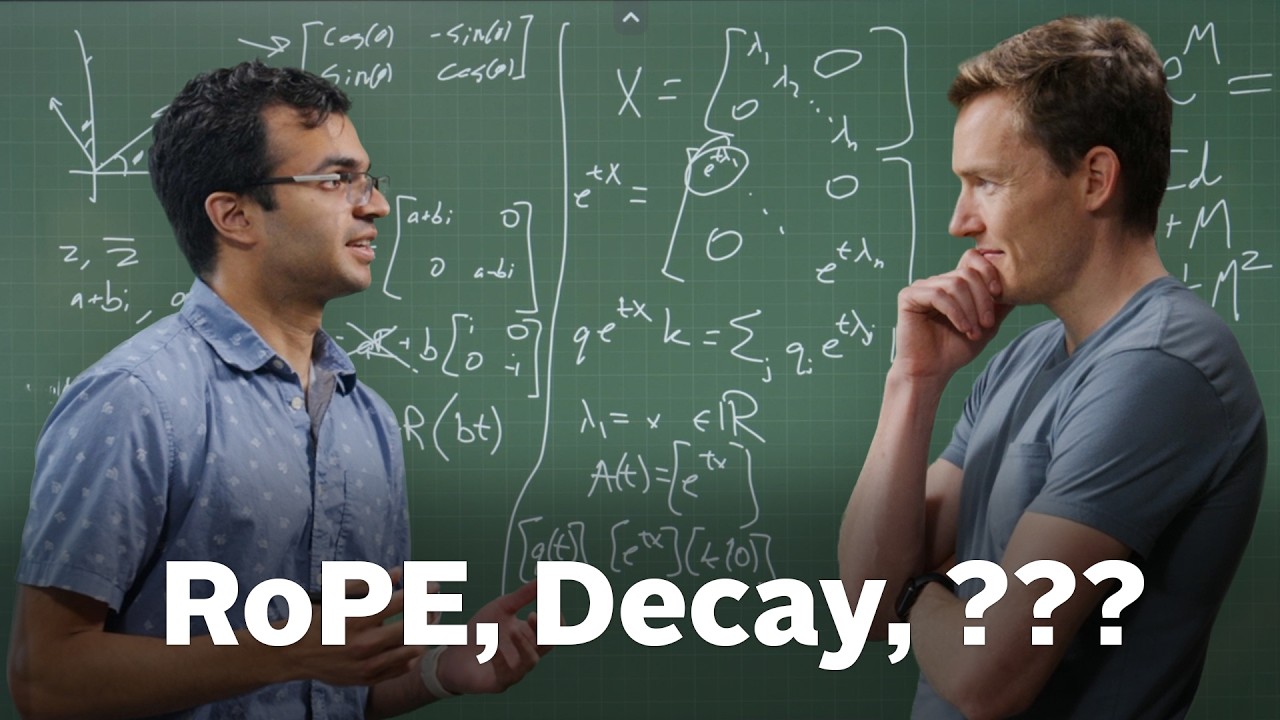
Jane Street Proves RoPE and ALiBi Exhaust Positional Encodings

Jane Street证实RoPE与ALiBi穷尽了主要位置编码形式 将李群理论应用于平移不变注意力机制，证明所有线性机制均可归约为矩阵指数，从而证实RoPE和ALiBi等现有设计已涵盖所有可行的架构。 Grant Sanderson与Alok Puranik通过将查询和键形式化为连续时间函数，深入探讨了如何严格地向Transformer注意力机制中引入位置信息。通过施加平移不变性和线性变换约束，他们证明位置交互构成了一个从标量时间加法到矩阵乘法的群同态，其唯一解为矩阵指数$e^{tX}$。对生成元矩阵$X$的分析表明：实特征值对应指数衰减或增长，共轭复数对产生旋转位置嵌入（RoPE）中的二维平面旋转，而不可对角化的亏损若尔当块则生成线性偏置注意力（ALiBi）中采用的线性距离惩罚。最终，这一数学分类表明现有的位置编码架构已自然穷尽了主要稳定的数学可能性。 通过在连续时间下构建查询与键的变换并施加平移不变性约束，位置编码可归约为一种将时间加法映射到矩阵乘法的群同态，其唯一解为矩阵指数A(t) = e^(tX)。 (28:27) 线性代数将位置编码的可能表现彻底归类为三种形态：基于实特征值的指数增长/衰减、基于共轭复数对的平面旋转（RoPE），以及基于亏损若尔当块的多项式偏移（ALiBi）。 (69:15) RoPE对应于实数衰减设为零的纯虚数可对角化情形，其在正交的二维子空间中部署几何频率谱，以防止跨序列长度时发生相位混叠。 (52:21) ALiBi的线性Logit惩罚可通过作用于增广坐标通道上的不可对角化2x2若尔当块在代数上复现，这证实了常见的经验性位置编码已涵盖了数学上可行的选项。 (69:15)

Analyzing transformer positional encodings through group representation theory reveals that assuming translation invariance and linearity inevitably restricts positional operators to matrix exponentials of the form $e^{sX}$. Through eigendecomposition and Jordan normal form, this unified algebraic framework completely classifies existing empirical methods into real exponential decay, RoPE rotations, and ALiBi linear penalties. First Principles: Linearity, Invariance, and Lie Generators (8:53) Standard transformer attention calculates query-key inner products without inherent awareness of token sequence order. To inject relative position while maintaining linear computational efficiency, positional modifications must act individually on each query $q(t)$ and key $k(s)$ via linear maps $F(t)$ and $G(s)$, rather than scaling quadratically over all $N^2$ token pairs. Enforcing translation invariance dictates that the interaction depends solely on relative offset: $A(t - s) = F(t)^T G(s)$, with the baseline condition $A(0) = I$ absorbing any uniform key transformations. Interpreting $A$ as an operator that bridges representations across continuous time leads directly to the group homomorphism $A(s)A(t) = A(s + t)$, converting additive temporal shifts into matrix multiplication. Differentiating this relation with respect to $t$ at $t = 0$ yields the matrix ordinary differential equation $A'(s) = A(s)X$, where $X = A'(0)$ acts as a constant generator. Given $A(0) = I$, the unique solution across continuous time is the matrix exponential $A(s) = e^{sX}$. Diagonalizable Generators: Exponential Decay and RoPE Rotations (38:41) Because time-invariant changes of basis can be absorbed by the surrounding neural network layers, the dynamics of $e^{sX}$ depend strictly on the canonical form of the generator $X$. For generic, diagonalizable matrices, $X$ decouples into independent one-dimensional and two-dimensional invariant subspaces without cross-talk. A real eigenvalue $\lambda = x$ yields a scalar factor $e^{tx}$. When $x < 0$, it produces exponential decay over time, mirroring the inductive bias found in recurrent neural networks and linear attention architectures (while $x > 0$ yields unstable exponential growth). In contrast, complex conjugate eigenvalue pairs $a \pm bi$ introduce planar rotations. Setting the real component to zero ($a = 0$) isolates pure rotations by angle $\theta = bt$. Stacking these $2 \times 2$ rotation blocks across a geometric spectrum of frequencies $\theta_k$ recovers Rotary Position Embeddings (RoPE), where fast frequencies resolve local word boundaries and slow frequencies track global context across thousands of tokens. Defective Matrices: Recovering ALiBi from Nilpotent Jordan Blocks (58:59) Beyond diagonalizable systems lies the measure-zero set of defective matrices, represented via Jordan normal form. For a defective $2 \times 2$ nilpotent generator with zeros on the diagonal and a 1 on the superdiagonal, the matrix squares to zero ($X^2 = 0$). Its Taylor series expansion terminates cleanly after the first degree, producing the linear polynomial $e^{tX} = I + tX = \begin{pmatrix} 1 & t \\ 0 & 1 \end{pmatrix}$. This structure governs dynamical kinematics equivalent to a frictionless body drifting at constant velocity. While unbounded linear growth initially appeared impractical for vector transformations, augmenting query and key vectors with fixed auxiliary entries maps this polynomial directly into attention logits. Sandwiching $I + tX$ between fixed components isolates an unscaled linear offset, mathematically reproducing the empirical distance penalty $-p(t - s)$ used in Attention with Linear Biases (ALiBi). The representation-theoretic formulation provides an exhaustive mathematical taxonomy that unifies linear attention decay, RoPE rotations, and ALiBi linear penalties under a single algebraic framework. Although higher-order Jordan blocks can mathematically generate quadratic or higher-degree polynomials, Alok Puranik concludes they hold little practical utility, indicating that machine learning practitioners have already identified the primary viable positional mechanisms.

Jane Street 研究员 Alok Puranik 与 Grant Sanderson 指出，主流 Transformer 位置编码并非孤立的经验设计，而是在平移不变性与线性假设下，通过群表示论推导出的矩阵指数族的必然特例。 公理化约束与同态群结构 (0:00) 原始自注意力机制仅通过 Query 与 Key 向量的内积来评估关联度，本质上对序列顺序完全脱敏，因此必须额外注入位置信息。为了避免每对 Token 独立变换所导致的二次方计算开销，Alok Puranik 将位置感知建模为对每个 Query 和 Key 向量分别进行的变换。此外，他将 Token 序列拓展为连续时间函数，这一设定不仅适用于自然语言离散标记，也能自然拓展至金融领域的高频非均匀数据以及 Mamba 等状态空间模型。 在将变换限定为线性映射后，两 Token 间的交互可表达为双线性形式。Alok Puranik 引入了平移不变性这一物理守恒思想：位置编码应仅取决于相对时间差，即存在矩阵函数满足双线性变换等于 $A(t - s)$，并在零位移时退化为单位矩阵 $A(0) = I$。通过平移性质复合两个时间步长，推导出核心同态恒等式 $A(s)A(t) = A(s+t)$。这意味着时间标量的加法群被保真地映射为矩阵的乘法群，从根本上锁定了其指数形式。 连续微分与生成元解耦 (28:27) 基于时间连续性的假设，Alok Puranik 在零点对群恒等式求导，直接导出了微分方程 $A'(s) = A(s)X$，其中生成元矩阵 $X = A'(0)$。结合 $A(0) = I$ 的初始条件，可以得出该系统的唯一闭式解为矩阵指数 $A(s) = e^{sX}$。Grant Sanderson 指出，任何与时间无关的基底变换都能被神经网络的前后线性层吸收，因此位置编码的研究可完全化简为在相似变换等价类下对生成元 $X$ 的分类探讨。 在生成元可对角化的通用情形下，整个多维交互解耦为互不干扰的一维与二维不变子空间之和。这意味着复合的注意力交互被还原为独立标量动态的累加，消除了不同维度间的交叉串扰。所有可能的时间演变特征，由此被完全限定在生成元特征值所决定的动力学范畴内。 特征值动力学对应的主流架构 (38:41) 可对角化生成元 $X$ 的特征值性质直接对应了业界现有的编码方案。当特征值为实数时，$e^{tx}$ 表现为纯粹的标量缩放：正实数会导致远古 Token 权重呈指数发散，在语言建模中极不稳定；零特征值对应与时间无关的稳态分量；负实数则表现为历史信息的指数衰减，这与 RNN 的隐式遗忘机制以及线性注意力模型中的衰减策略完全吻合。 当特征值为共轭复数对时，二维实子空间上的动力学转变为平面旋转与缩放的组合。当把衰减项设为零时，系统便严格退化为纯旋转矩阵块，这正是主流 Rotary Positional Embedding (RoPE) 的底层数学本质。RoPE 选取的几何级数频率分布实质上构建了一套多尺度时钟：高频分量用于精细区分相邻几个 Token 的微小位移，低频分量则跨越数千 Token 捕捉全局语义上下文，防止相位循环包裹引发的位置混淆。 非对角化缺陷矩阵与 ALiBi (58:59) 对于测度为零但在代数分类中不可或缺的不可对角化矩阵，系统可以通过若当标准型进行刻画。Alok Puranik 以对角线为零的二维幂零若当块为例，其平方直接为零。代入泰勒级数展开后，高阶项全数归零，使矩阵指数坍缩为线性的多项式形式 $I + tX$。从物理直觉来看，这等价于无外力作用下的匀速滑块运动，其位移随时间线性漂移。 这种随距离线性增长的动力学看似会导致注意力发散，但 Alok Puranik 证明，如果在原始 Query 和 Key 向量末端拼接固定的常数辅助维度，该幂零矩阵在双线性相乘后即可精准产生一个与时间差成正比的线性偏置项 $-p(t - s)$。这一推导在数学上严格还原了此前被视为外生启发式惩罚的 ALiBi 机制，完成了从连续群表示向非对角化结构的技术闭环。 Alok Puranik 与 Grant Sanderson 的推演表明，主流位置编码（RoPE、指数衰减线性注意力和 ALiBi）已经穷尽了矩阵指数群分类中的实指数、复旋转和一次多项式三种基本形态；虽然更高阶的不可对角化若当块能在理论上构造二次或更高阶的时间惩罚，但在实际注意力模型中缺乏明显的工程效用与突破潜力。

## Background 该视频由 Jane Street 于 2026 年 8 月 26 日在 YouTube 平台发布。视频中，3Blue1Brown 的 Grant Sanderson 与 Jane Street 研究员 Alok Puranik 围绕后者发表的技术博客展开讨论，从注意力机制的基本假设出发，借助群论与表示论系统探讨 Transformer 位置编码的可能数学形式，并将其与 RoPE 及 ALiBi 等现有方法紧密联系起来。 ## TL;DR 对话从注意力机制固有的置换不变性以及引入位置编码的必要性切入，通过对 Query 和 Key 施加单目独立变换、线性映射及平移不变性等自然公理，推导出了相对位移矩阵满足的柯西柯西柯西函数方程 $A(s+t) = A(s)A(t)$。随后，借助连续时间可微性，二人证明了该位移算子必然具有矩阵指数 $e^{tX}$ 的形式，并将整个位置编码空间严格收敛至该李群结构中。通过对生成元矩阵 $X$ 进行对角化与特征值分析，他们代数化地复现了一维指数衰减以及 RoPE 的多尺度二维块旋转；而针对不可对角化的幂零若尔当块（Jordan block），他们进一步结合冰球运动动力学，通过状态向量增广成功推导并统一了 ALiBi 的线性偏置惩罚项，最终在纯代数视角下论证了主流位置编码方案的完备性与理论边界。 ## Atmosphere & style 整场对话呈现出一种兼具严密数学推导与随性极客茶歇气息的“白板讨论”氛围。Grant Sanderson 扮演着兼具敏锐直觉与幽默感的苏格拉底式提问者，不断用物理类比和形象几何图景拆解高深代数，而 Alok 则在白板前层层推进，在遭遇复杂项时坦率分享推导中的弯路与试错。从最初面对抽象矩阵指数时的思维震撼，到看穿对角化本质后的豁然开朗，再到最终将冷门的若尔当块精准拼回 ALiBi 的顿悟瞬间，整个过程充盈着对数学对称之美与第一性原理统一性的智力满足感。 ## Bulletin - [28:27](https://www.youtube.com/watch?v=k86eUj4hgdc&t=1707s) Jane Street 研究员 Alok Puranik 与 Grant Sanderson 合作，基于群表示论推导证明，在平移不变性和独立单目线性变换等极小假设下，Transformer 的相对位置编码矩阵族必然服从矩阵指数形式 A(t) = exp(tX)。 - [52:21](https://www.youtube.com/watch?v=k86eUj4hgdc&t=3141s) 推导展示了主流位置编码在代数上的统一性：实特征值对应指数衰减（如线性注意力），成对的虚特征值对应正交旋转（RoPE），而不可对角化的若尔当块则生成线性项并可精确等价还原出 ALiBi。 - [01:13:42](https://www.youtube.com/watch?v=k86eUj4hgdc&t=4422s) 该数学框架完整刻画了合理位置编码的理论解空间，表明当前深度学习领域几乎已遍历了所有稳定形式，未被探索的高阶若尔当多项式在实际应用中缺乏数值稳定性与实用价值。 ## Key takeaways - [02:34](https://www.youtube.com/watch?v=k86eUj4hgdc&t=154s) 标准 Transformer 注意力机制计算 Query 和 Key 的点积打分，但天然具备置换不变性，缺少感知时序和绝对/相对位置的能力。 - [03:54](https://www.youtube.com/watch?v=k86eUj4hgdc&t=234s) 采用连续时间函数 q(t) 和 k(s) 建模序列，不仅符合物理世界的现实时序采样，也为引入微分方程与李代数工具提供了数学基础。 - [07:02](https://www.youtube.com/watch?v=k86eUj4hgdc&t=422s) 为保持计算复杂度在 O(n) 而非膨胀至 O(n²)，模型对 Query 与 Key 施加独立的单目位置变换，并合理假设该变换为有限维线性矩阵乘法。 - [11:18](https://www.youtube.com/watch?v=k86eUj4hgdc&t=678s) 平移不变性要求注意力的时间依赖仅取决于相对时间差 (t - s)，将原本二维参数网格 F(t)ᵀ G(s) 沿对角线坍缩为一维位移矩阵族 A(t - s)。 - [20:45](https://www.youtube.com/watch?v=k86eUj4hgdc&t=1245s) 结合零位移规范化条件 A(0) = I，利用平移不变性消除逆元项，推导出矩阵代数复合性质 A(s)A(t) = A(s + t)。 - [28:27](https://www.youtube.com/watch?v=k86eUj4hgdc&t=1707s) 在 t = 0 处对连续时间求导，微分方程 A'(s) = A(s)X（其中 X = A'(0)）直接导出了矩阵指数解 A(s) = exp(sX)。 - [38:41](https://www.youtube.com/watch?v=k86eUj4hgdc&t=2321s) 通过对可对角化矩阵 X 的分析，注意力内积解耦为若干独立子空间，其实数特征值 x 对应着平坦常数（x=0）、指数增长（x>0）或指数衰减（x<0）。 - [44:05](https://www.youtube.com/watch?v=k86eUj4hgdc&t=2645s) 实数矩阵的共轭复特征值对可分解为缩放项与纯旋转项，当令实部衰减系数为 0 时，即构成了 RoPE（旋转位置编码）所依赖的刚性二维旋转对角块。 - [55:04](https://www.youtube.com/watch?v=k86eUj4hgdc&t=3304s) RoPE 在各个二维子空间中设置按几何级数递减的旋转角速度，本质上是为模型构建了一组兼顾局部高分辨率与长程跨度的“多时钟系统”。 - [01:02:08](https://www.youtube.com/watch?v=k86eUj4hgdc&t=3728s) 针对不可对角化矩阵，以 2×2 若尔当块为例，其幂零性使得矩阵指数的高阶泰勒级数精确截断，生成与时间相关的线性多项式动力学（如无摩擦冰球运动）。 - [01:09:15](https://www.youtube.com/watch?v=k86eUj4hgdc&t=4155s) 通过对 Query 和 Key 向量追加特定的常数维度，带有若尔当块的不可对角化算子能够完美在代数上复现主流的 ALiBi（线性偏置注意力）惩罚项。 - [01:13:42](https://www.youtube.com/watch?v=k86eUj4hgdc&t=4422s) 该推导为位置编码的数学形态划定了理论边界，证实学术界和工业界目前主流的 RoPE、ALiBi 及线性衰减已经覆盖了大部分稳定、合理的表示空间。 ## Detailed walkthrough ### [00:00](https://www.youtube.com/watch?v=k86eUj4hgdc&t=0s) 表示论的视角：从 RoPE 与线性注意力谈起 Jane Street 的研究员 Alok Puranik 与 3Blue1Brown 的 Grant Sanderson 展开对话。Alok 谈到自己平时阅读大量深度学习前沿论文，试图跟进各种新型网络架构，过程中经常遇到各式各样的位置编码变体。在这些方案中，RoPE（Rotary Positional Embedding，旋转位置编码）凭借其优雅的数学性质，几乎成了当前大语言模型的事实标准。RoPE 的核心操作是将向量坐标两两配对，并让它们随着时间进行旋转，把时间信息编码为一组旋转变换。 对于具有表示论（Representation Theory）背景的人来说，这种将实数加法群 $(\mathbb{R}, +)$ 或整数加法群 $(\mathbb{Z}, +)$ 映射为具有同构结构的矩阵算子的做法，可以说是再熟悉不过的数学套路。Alok 敏锐地察觉到，类似的想法也出现在其他地方：例如在线性注意力（Linear Attention）中，模型并非通过坐标旋转来编码时间，而是通过指数衰减来抑制旧的信息。表面上看两者截然不同，但深究其数学内核，它们本质上是同一种代数结构的体现。Grant 提到，大多数论文在提出这类位置编码时，往往只是将其作为一种“足够自然的选择”，而 Alok 的博客文章则反其道而行之，从第一性原理追问：“它必然是什么样的？现存的所有方法是否只构成了这庞大表示空间的一个子集？是否还存在从未被探索过的新方法？” Alok 解释了自己当初展开这一探索的动机：“It felt like it couldn't be a coincidence that like two very popular methods came from this same like said both had this algebraic structure and now then the natural question is like maybe all of the methods have this algebraic structure is there some like what's the kind of the minimal set of assumptions that gives you this and like do they seem like reasonable assumptions something like that.” ### [02:34](https://www.youtube.com/watch?v=k86eUj4hgdc&t=154s) 注意力机制的双刃剑：置换不变性与位置的缺失 在深入数学推导前，Grant 调出自己视频中的动画示意图，回顾了注意力机制的核心问题。在 Transformer 架构中，输入的词嵌入（Embeddings）分别被投影为一系列 Query 向量与 Key 向量。当模型在处理类似“一只毛茸茸的蓝色生物在茂密的森林中漫步（a fluffy blue creature roamed the verdant forest）”这样的句子时，形容词“fluffy”和“blue”需要确定自己应该将注意力投向名词“creature”。这一交互强度完全是通过计算 Query 和 Key 之间的点积来衡量的。 注意力机制的核心魅力在于其不对时间做预先假设——它不会武断地认为“前一个词一定比更早的词重要”，所有的关联权重都由模型端到端学习而来。然而，这种与顺序无关的置换不变性也是注意力机制的“阿喀琉斯之踵（Achilles' heel）”。在语言和现实序列中，相对位置和绝对次序极其关键。模型必须要在仅使用矩阵运算的框架内，找到一种能够表达“我在序列中所处位置”的通用机制。 ```mermaid flowchart LR accTitle: Transformer Attention with Position Flow accDescr: An overview showing how embeddings become queries and keys and where time/position must be incorporated before dot product attention. subgraph Inputs ["序列输入与投影"] E["Token 嵌入序列"] --> Q["Query 向量"] E --> K["Key 向量"] end subgraph PosEnc ["位置注入环节"] Q --> Q_mod["加入时间/位置 t 的调制"] K --> K_mod["加入时间/位置 s 的调制"] end subgraph Scoring ["注意力计算"] Q_mod --> Dot["点积打分 (Query · Key)"] K_mod --> Dot Dot --> Attn["注意力权重 (置换不敏感被打破)"] end ``` ### [03:54](https://www.youtube.com/watch?v=k86eUj4hgdc&t=234s) 建模起步：引入连续时间函数表达 为了建立起最普适的数学框架，Alok 并没有采用常规离散序列的写法（即 $Q_1, Q_2, \dots, Q_N$），而是做出了一个更加广义的选择：将 Query 和 Key 视为关于时间的函数 $q(t)$ 与 $k(s)$，其中时间参数满足 $0 \le t \le T$。如果令 $t, s$ 取离散整数，该体系立刻退化为标准离散序列模型。 Grant 对此提出疑问，好奇这是否源于金融领域研究者（如 Jane Street）处理高频或非规则市场行情数据的职业习惯，因为现实物理世界和金融时序往往不是规整的离散步长。Alok 承认了这一点，指出真实世界物理现象在连续时间下建模更为自然，只需在感兴趣的时刻进行采样即可；同时，近期的热门架构如 Mamba 等状态空间模型（SSM）也采用了类似的连续时间表述。此外，连续时间的框架未来还能自然推广到数据驱动的自适应衰减率等高级场景中。 在接下来的推导中，Alok 明确表示他们将暂时忽略 Value 向量的聚合计算，将所有精力聚焦在决定注意力分布的核心——Query 与 Key 的点积打分上： - 目标是评估位于时刻 $t$ 的 Query 对位于时刻 $s$ 的 Key 赋予多少注意力权重。 - 标准的打分方式是直接计算点积：$q(t)^T k(s)$。 - 这一基础点积存在致命缺陷：若 $k(0)$ 与 $k(1)$ 的向量数值相同，点积结果将毫无二致，模型完全无法感知它们在时间轴上的距离与位置差异。 ### [07:02](https://www.youtube.com/watch?v=k86eUj4hgdc&t=422s) 独立变换假定：$O(n)$ 与 $O(n^2)$ 的效率权衡 为了让点积感知时间，必须引入时间依赖的修正函数。Alok 提出了第一层假设：直接对 Query 和 Key 进行显式的时间依赖变换，即构造修改后的向量： - 变换后的 Query：$\tilde{q}(t) = f(t, q(t))$ - 变换后的 Key：$\tilde{k}(s) = g(s, k(s))$ 在原始的 Transformer 架构中，这一变换体现为在原始向量上直接叠加正弦与余弦位置编码（Sinusoids）；而在 RoPE 中，这一变换则是利用正交矩阵对向量进行二维平面旋转。 Alok 专门解释了为何设定 $f$ 和 $g$ 仅依赖各自的单点时间（每个 Query 和 Key 仅被修改一次，处理 $n$ 个对象），而不是针对所有两两组合的 $(t, s)$ 构造一套修改全量点积的二元函数（处理 $n^2$ 对相互作用）： - “It's very likely impractical to blow that up into like n squared queries and n squared keys where you modify them differently for every single pair of times.” - 序列长度为 $n$ 时，维护 $n$ 个 Query 和 $n$ 个 Key 的线性修改在计算和内存效率上是实际可行的；若为每一对时间跨度引入定制化调制，计算开销将膨胀到不可接受的 $n^2$ 量级。 - 这一“每个 Query/Key 各自独立进行单目变换”的设定，构成了后续所有群论推导的重要起点，Grant 也赞许这种在追求极致数学一般性的同时兼顾工程现实边界的权衡。 ### [08:53](https://www.youtube.com/watch?v=k86eUj4hgdc&t=533s) 从点积到函数约束：为什么必须做线性假设 在引入带有波浪号（twiddle）的时间感知变换向量 $\tilde{q}(t)$ 与 $\tilde{k}(s)$ 后，注意力权重的核心运算落在了内积 $\tilde{q}(t)^T \tilde{k}(s)$ 上。Grant Sanderson 随性打趣道，他们目前其实还没证明任何东西，只是在上一节的表达式头上加了波浪号，试图把形式先写下来让其“更具时间感知”。但 Alok Puranik 指出，若允许 $f$ 和 $g$ 保持为完全任意的数学函数，它们可能会极端恶劣、毫无规律，导致理论分析根本无从下手。为了构建严谨的推导，必须对其施加限制。 ```mermaid flowchart LR accTitle: Linearization of Positional Transformations accDescr: Mapping arbitrary functions f and g to indexed matrix families via linearity assumption. subgraph Raw["任意函数空间 (无穷维)"] F1["f(q(t), t)"] G1["g(k(s), s)"] end subgraph Linear["线性映射假设 (有限维)"] F2["F(t) ∈ R^(d×d)"] G2["G(s) ∈ R^(d×d)"] end Raw -->|"施加线性约束"| Linear ``` Alok 提出的第一个关键约束是**线性（Linearity）**。虽然在纯数学层面上严格证明“为何现实必须是线性的”并不容易，但在向量内积空间这一天然语境下，线性映射是处理向量与点积最和谐的工具。Alok 坦言：“在实践中，我发现没有任何现有工作会在这一步使用非线性映射，这让我更加确信：没有人会因为做出这个假设而感到难过，所以它大概率完全行得通。”Grant 对这种在追求完全普遍性与工程实际之间的适度权衡深表赞同，认为将 $f$ 写成一个依赖于时间 $t$ 的矩阵作用在 $q$ 上，在注意力机制的背景下显得自然且不可避免。 - **降维简化**：从不可控的连续任意函数，转化为以时间参数为索引的矩阵族 $F(t)$ 与 $G(s)$。 - **参数规模**：若在 $d$ 维嵌入空间中运算，原本无法量化的函数形态被精确收缩为 $d^2$ 个受时间调控的数值集合。 - 具体的变换形式由此确定为：$\tilde{q}(t) = F(t) q(t)$，$\tilde{k}(s) = G(s) k(s)$。 --- ### [11:18](https://www.youtube.com/watch?v=k86eUj4hgdc&t=678s) 二次型视角与平移不变性公理 将线性矩阵代入原本的点积式中，查询向量与键向量之间的匹配关系立刻展开为一个清晰的二次型（quadratic form）：$q(t)^T \left( F(t)^T G(s) \right) k(s)$。这一小块夹在中间的乘积 $F(t)^T G(s)$，完全定义了 $t$ 时刻的 query 与 $s$ 时刻的 key 之间如何进行几何配对。然而，若乘积依赖于两个各自孤立的时间刻度 $t$ 与 $s$，系统依旧缺乏结构性。因此，Alok 引入了驱动后续所有推导的核心引擎——**平移不变性（Translation Invariance）**。 其背后的物理直觉极为朴素：位置编码的效果理应只取决于两个 token 之间的相对时间差（相对位移）。第 10 个 token 看待第 5 个 token 的相对注意方式，应当与第 110 个 token 看待第 105 个 token 的方式完全一致。Grant 感叹这具有浓厚的理论物理色彩，宛如诺特定理（Noether's theorem）中“对称性带来守恒量或强约束”的思想重现。为此，Alok 正式定义了相对位移矩阵 $A(t - s)$： $$A(t - s) = F(t)^T G(s)$$ 从几何与语言直觉来看，矩阵 $A$ 扮演着“时间演化算子”的角色。设想某个在 $s$ 时刻的 key 编码了一个形容词，我们不能直接将处于不同时间点的向量做内积，而必须依靠算子 $A$ 将该 key 沿时间向前推进至 $t$ 时刻的几何空间中；$A$ 的取值精确量化了“当向前跨越特定时间步长后，过去的信息对未来的 query 还能保留多少影响力”。随着步长拉大，这种语言修饰作用可能会逐渐衰减甚至失效。 > “我们真正希望的是，这种位置编码的效果仅仅取决于时间差。第 10 个 token 看待第 5 个 token 的方式，理应与第 110 个 token 看待第 105 个 token 的方式完全相同。” —— Alok Puranik --- ### [14:47](https://www.youtube.com/watch?v=k86eUj4hgdc&t=887s) 规范化约束：零位移的单位矩阵与相伴不变性 为了让算子 $A$ 具有规范的物理与几何基准，Alok 进一步要求 $A(0) = I$（单位矩阵）。从直觉上看，当相对时间差为零（即 query 与 key 处于同一时刻）时，没有任何信息被推进或跨越时间，因此系统不对原始点积做任何改动，即 $q(t)^T k(t)$ 保持未被扭曲的原貌。Alok 补充论证了该假设并未损失一般性：若设 $A(0) = M$（$M$ 为某一非单位的可逆矩阵），我们完全可以通过定义 $\tilde{k}'(t) = M k(t)$，将该矩阵作为一个与时间无关的全局变换吸收进 key 的投影参数中，从而在不改变时间依赖本质的前提下强行归一化出 $A(0) = I$。 ```mermaid flowchart TD accTitle: Dimensional Collapse and Invariance accDescr: Collapsing the two-parameter function F(t)^T G(s) onto counter-diagonals where t minus s is constant. subgraph TwoD["双参数网格 (t, s)"] Grid["F(t)^T G(s)"] end subgraph Invariance["平移不变性折叠"] Diag["沿反对角线坍缩: (t - s) 为常数"] end subgraph OneD["一维矩阵族 A(t - s)"] Base["A(0) = I (同时间基准)"] Shift["A(t - s) = F(t - s)^T G(0)"] end Grid -->|"施加平移不变性"| Diag Diag -->|"标准化对齐"| OneD ``` Grant 借用坐标图景给出了形象的几何概括：在 $(t, s)$ 的坐标网格中，如果内积算子只由时间差决定，那么凡是满足 $t - s$ 为常数的沿对角线/反对角线轨迹上的矩阵值都是恒定的。整个双参数平面因此被坍缩（collapse）到一维的相对距离轴上：$A(0)$ 描述的是所有对角线上的自身重合关系，$A(-1)$ 则代表将信息往回拨动一个单位。 - **规范化条件**：$A(0) = I$，确立了无时间差时的天然单位度量。 - **平移不变性公式**：精确表述为 $F(t)^T G(s) = F(t - s)^T G(0) = A(t - s)$。这表明任意两点的交叉积，均可等价映射为相对于零点的单变量位移矩阵。 - **反解的自由度**：只要给定了合法的矩阵族 $A$，在忽略某个全局正交旋转的前提下（该旋转在内积中相互抵消），便能直接反解出原本的变换矩阵族 $F$ 与 $G$。 当 Grant 敏锐地发问“这是否意味着我们可以随意挑选任意随时间变化的矩阵 $A$ 来发明属于自己的位置编码”时，Alok 笑着指出事情没有那么简单：由于变换必须由 $F(t)$ 和 $G(s)$ 的外积形式分解而来，矩阵族 $A$ 自身必须严格满足深层的内在代数一致性条件。这也是引入群论与表示论进行分类探索的根本契机。 ### [18:47](https://www.youtube.com/watch?v=k86eUj4hgdc&t=1127s) 逆关系与两个 $A$ 矩阵相乘的直觉飞跃 在回顾先前的推导后，Alok Puranik 总结指出：$f(t)^\top g(t) = A(0) = I$（单位矩阵），由此直接得到了 $f(t)$ 与 $g(t)$ 之间的求逆关系，即 $f(t)^\top = g(t)^{-1}$。 紧接着，Alok 指出这里需要完成一次思维上的“直觉飞跃”：去计算两个 $A$ 矩阵的乘积 $A(s)A(t)$，观察会发生什么。从实际工程计算注意力权重的角度来看，这绝非显而易见之举。因为在硬件计算注意力分数的流水线中，根本没有任何一步需要将两个 $A$ 矩阵直接相乘。然而，如果将 $A$ 视为从时间点 $0$ 到时间点 $t$（或从时间点 $s$ 到时间点 $t$）的“桥梁”，那么走过一次桥梁，紧接着再走第二次桥梁跨越到另一个时间，去探究其复合效果就是极其自然的代数冲动。 Grant Sanderson 笑着调侃，熟悉群论的人往往带着一种“令人愉悦的放飞心态”去提问，完全不顾硬件里是否真的存在这样的计算操作。Grant 认为这完全合理：“这对我来说很说得通。你只是想理解理论上 $A$ 应该是什么。”（“Makes sense to me. So you're just trying to understand the theory of what A should be.”）Alok 也赞同道：“是的，就算它从未在实际应用中真正出现过，从结构上看这也是一个非常自然需要回答的问题。”（“yeah, it's like a structurally natural question to answer even if it never like quite shows up in the practical application we're we're looking for.”） ```mermaid flowchart LR accTitle: Matrix Composition Interpretation accDescr: Diagram showing how A of s and A of t compose as temporal transitions to yield A of s plus t. subgraph Transitions["时间状态转移"] T0["位置 0"] -->|"A(s)"| TS["位置 s"] TS -->|"A(t)"| TST["位置 s + t"] T0 -.->|"A(s + t)"| TST end ``` --- ### [20:45](https://www.youtube.com/watch?v=k86eUj4hgdc&t=1245s) 代数展开与平移不变性的巧妙消除 对于 $A(s)A(t)$ 的乘积，直觉预期它应当等于 $A(s+t)$，因为 $A(s)$ 代表从 $0$ 移动到 $s$，而 $A(t)$ 代表再移动 $t$ 的位移。为了在代数上验证这一点，Alok 使用了基于平移不变性的具体定义式：$A(t) = f(t)^\top g(0)$。将两项展开后得到： $$A(s)A(t) = f(s)^\top g(0) f(t)^\top g(0)$$ 中间项 $g(0) f(t)^\top$ 看起来有些别扭，但利用平移不变性，对于配对出现的 $f^\top$ 与 $g$，可以自由地对内部参数同时加减相同的偏移量而不改变结果。Alok 将左侧那一对参数整体平移 $+t$： - $f(s)^\top \to f(s+t)^\top$ - $g(0) \to g(t)$ 此时整个表达式变形为： $$f(s+t)^\top g(t) f(t)^\top g(0)$$ 此时中间赫然出现了 $g(t) f(t)^\top$。由于之前已经确立了 $f(t)^\top = g(t)^{-1}$，中间两项互为逆矩阵，正好彻底抵消为单位矩阵 $I$。最后剩下的便是： $$f(s+t)^\top g(0) = A(s+t)$$ Grant 对这一步极为赞赏，称赞这种利用平移推进加上 $A(0)=I$ 的逆元消除非常漂亮。Alok 则坦诚自嘲，这种做法略有一点“循环论证”的意味——自己预先设定了一套强加该结构的基本假设，最后又惊叹“哇，这套结构居然自己弹出来了”。但他强调，这正是花大量时间阐明假设合理性的原因：在添加了大家普遍接受的约束后，就会得到一个极其紧凑、刚性的数学对象。 - $A(t)$ 的等价定义形式：$A(t) = f(t)^\top g(0)$ - 依据平移不变性：$f(s)^\top g(0) = f(s+t)^\top g(t)$ - 逆元消除：$g(t) f(t)^\top = I$ - 导出核心性质：$A(s)A(t) = A(s+t)$ --- ### [24:32](https://www.youtube.com/watch?v=k86eUj4hgdc&t=1472s) 自变量加法转矩阵乘法：指数映射与图像 Transformer 的联想 Alok 指出，方程 $A(s+t) = A(s)A(t)$ 是后续一切推导的真正核心。对于任何哪怕不懂群论或表示论的人来说，只要“眯起眼睛”暂时忘掉 $A$ 是个矩阵，看到自变量的加法变成函数值的乘法，脑海里第一反应必然是——指数函数（Exponential）。但在高中代数里这只适用于实数，而当 $A$ 是矩阵时，除非有物理学或表示论背景，否则其含义并不直观。 Grant 随即追问 Alok 当初推导的心路历程：究竟是逻辑顺推推导出了指数，还是倒推法？即先观察到很多现有的位置编码（如 RoPE 等）都带有一种指数或旋转的气息，然后试图为其寻找理论证明？Alok 承认自己最初确实是倒推思考： > “是的，我觉得我绝对是从……你知道的，当你阅读所有这些文献时，你会想：好的，有些包含了真正的指数，有些包含了旋转，而旋转其实就是复指数。所以，这些东西肯定是有由来的。”（“Yeah, I think I I definitely started by like, you know, when you read all this literature, you like you go like, okay, some of these have actual exponentials, some of these have rotations, which are really just complex exponentials. So, like these have got to be coming from somewhere.”） Alok 进一步补充道，在位置编码中使用群表示理论，自己绝非首创。特别是在图像处理的视觉 Transformer（Vision Transformer）中，位置并非一维的单一移动方向，而是二维结构。为了保证在复合两个维度的位置编码时行为合理，研究者通常会借助类似的数学工具，确保构建出加法群直和 $\mathbb{R} \oplus \mathbb{R}$ 的群表示。 --- ### [27:12](https://www.youtube.com/watch?v=k86eUj4hgdc&t=1632s) 对 $t=0$ 处求导：连续时间假设的真正价值 在黑板上清理出一块空间后，Alok 开始展示一个“不太严格但极具直观性”的证明，旨在揭示为什么这里必然导出矩阵指数。 由于 $A$ 在注意力机制中充当夹在查询（Query）和键（Key）嵌入向量之间的“桥梁”以吸收时间差异，Alok 假设映射 $A(t)$ 是可微的，并考虑在 $t=0$ 附近对参数 $t$ 求导。选择在 $t=0$ 处展开求导的原因非常务实：因为 $0$ 是目前唯一确定了 $A$ 具体取值（$A(0)=I$）的锚定点。 Grant 随即指出，这生动展示了将位置/时间视为连续变量的优越性：“顺便说一句，这正是把时间视为连续变量的一个极佳理由。如果你只是给出整数索引，根本不可能问出这样的问题。”（“which is a side note is just a great justification for why thinking of time continuously like this would not be a question to ask if you were just giving like integer indices.”）Alok 笑着赞同，如果完全局限在整数离散索引下，推导固然可以通过步进相乘简化，但连续视角与微积分工具直接为李群和李代数（Lie group / Lie algebra）风格的指数解法打开了大门。 ### [28:27](https://www.youtube.com/watch?v=k86eUj4hgdc&t=1707s) 从微分方程推导矩阵指数解 Alok Puranik 和 Grant Sanderson 正在黑板上推导位置编码的代数形式。Alok 调侃道，从 0 开始通过不断加 1 就能到达任何位置，这在某种意义上简单得多；Grant 接着打趣说：“好吧，我们这是令人愉悦地……不，这不算过度复杂，这叫具有一般性（well we're being delightfully uh not it's not over complicated it's general）。”随后他们将等式设定在 $t = 0$ 处求导展开。 左侧表达式中，$A(s)$ 项作为系数不受影响保留下来，而 $A(t)$ 在 $t = 0$ 处的导数变成了 $A'(0)$；右侧直接求导得到 $A'(s)$。Grant 询问为什么不直接简写为 $A'(0)$，Alok 承认这样写确实更加清爽。至此，核心结构显现出来：导数等于某个常数矩阵乘以函数自身。他们将常数矩阵 $A'(0)$ 记作 $X$，方程化为 $A(s)X = A'(s)$。如果这是一个实数域上的常微分方程，解显然是指数函数。在矩阵代数中，这也正是矩阵指数（Matrix Exponential）的标准定义方式。 因为初始条件满足 $A(0) = I$（单位矩阵），方程的特解非常简洁：$A(s) = e^{sX}$。Grant 指出，一般人看到矩阵写在指数位置上（$e^{sX}$）可能不会立刻明白其含义，其实质就是泰勒级数展开： $$e^{sX} = \sum_{k=0}^{\infty} \frac{(sX)^k}{k!} = I + sX + \frac{1}{2}(sX)^2 + \frac{1}{6}(sX)^3 + \cdots$$ 只要是方阵，高阶幂运算便良定义。懂行的人可能会追问级数收敛性，而更深入的理解则需要结合特征值来考量。Alok 补充强调，这个展开式极其关键，因为后续探究位置编码内部究竟在发生什么时，必须借助它来拆解细节。 - 方程形式：$A'(s) = A(s)X$，其中 $X = A'(0)$。 - 初始条件：$A(0) = I$。 - 形式解：$A(s) = e^{sX}$。 ### [32:05](https://www.youtube.com/watch?v=k86eUj4hgdc&t=1925s) 实数、复数与矩阵动力学的类比 求得 $A(s) = e^{sX}$ 后，Alok 指出，在给定的几条自然假设下，全部合法的位置编码解空间已经被这个矩阵指数完全锁定了。现在的核心任务是刻画这个空间：能不能从中找出已知的经典编码方法？又能不能发现尚未被人探索过的新结构？ Grant 用标量常微分方程进行类比：在实数域中，解为 $e^{ct}$。当常数 $c$ 为正时，对应指数增长（growth）；当 $c$ 为负时，对应指数衰减（decay）。如果允许复数介入，常数 $c$ 可以是纯虚数，此时便引入了旋转（rotation）。在实数与复数构成的熟悉世界里，定性行为无非就是增长、衰减与旋转这三类。因此，当进入矩阵的世界时，问题就变成了：取决于我们如何选取矩阵 $X$，在增长、衰减与旋转的基础上，系统还能展现出怎样更丰富的动力学行为？Alok 赞同这一视角，指出任何实数都可以通过乘以单位矩阵升格为矩阵并复现这三类行为，但矩阵维度更高，其中蕴藏的可能性远不止于此。 ```mermaid flowchart TD accTitle: Dynamics of Exponential Solutions accDescr: Scalar versus matrix dynamics for exponential differential equation solutions. subgraph Scalar["标量情况: e^(ct)"] direction TB S1["c > 0: 指数增长 (Growth)"] S2["c < 0: 指数衰减 (Decay)"] S3["c 为虚数: 旋转变换 (Rotation)"] end subgraph Matrix["矩阵情况: e^(tX)"] direction TB M1["实数倍单位矩阵 cI: 复现实数动力学"] M2["斜对称矩阵 / 虚数特征值: 高维旋转 (RoPE)"] M3["一般矩阵结构: 耦合交互与更广阔的编码空间"] end Scalar -->|"升格扩展"| Matrix ``` ### [33:28](https://www.youtube.com/watch?v=k86eUj4hgdc&t=2008s) 基底变换不变性与特征值对角化 为了简化后续分析，Alok 引入了一个关键假设：Query 与 Key 的基底变换（Change of Basis）对注意力机制没有本质影响。如果在特征空间中对 Query 施加一个与时间无关的固定正交/旋转矩阵变换，从位置编码的角度来看这完全是一个空操作（noop），因为神经网络自身的线性层权重完全可以吸收并抵消掉这个变换。由于基底变换对 $X$ 的作用与对 $A$ 的作用形式完全一致，内积运算中的基底矩阵会相互抵消，因此研究人员只需要在“相差一个基底变换”的等价类意义下来考察矩阵 $X$。 在线性代数中，面对基底变换不敏感的矩阵指数运算，最自然的技术路径就是对角化（Diagonalization）。Alok 假设矩阵 $X$ 可对角化，其主对角线上的特征值为 $\lambda_1, \lambda_2, \dots, \lambda_n$。对角矩阵的指数运算极易处理，非对角元素全为零，指数映射直接作用于对角线的各个标量： $$e^{tX} = \begin{bmatrix} e^{t\lambda_1} & & 0 \\ & \ddots & \\ 0 & & e^{t\lambda_n} \end{bmatrix}$$ 当计算注意力内积项 $Q e^{tX} K$ 时，不同维度分量之间完全解耦。Query 的第 $j$ 个分量 $q_j$ 与 Key 的第 $j$ 个分量 $k_j$ 仅通过 $e^{t\lambda_j}$ 发生作用，与其他分量之间没有任何非对角交叉。Grant 进一步直观解释：对角矩阵求平方只需对角元素平方，求三次方也只是对角元素立方，泰勒展开原本复杂的高阶矩阵乘积混合在对角基底下一扫而空；选择特征基底本质上是将高维空间分解到了互不相干的一维子空间中。 Alok 将内积展开写成了标量求和形式：$\sum_j q_j e^{t\lambda_j} k_j$。Grant 特别感慨道，尽管写成标量指数和矩阵指数在符号形式上看似相似，但人的心理感受截然不同：“而且我想强调的是，虽然符号上看起来非常相近，但把指数位置上的东西看作算子，与把它看作纯粹的数字，内心感受是完全不同的；因为如果它是一个数字，我们确切地知道它在做什么——它要么增长，要么衰减，要么旋转（And I'll emphasize even though like symbolically it sort of looks very similar, like there's a very different emotion in thinking about that as being an operator in the exponent versus thinking about it as just being a number because like this one, like, oh, it's a number. We know what that does. It's like it grows, it decays, or it rotates）。” - 基底变换等价性：如果线性层能学出任意旋转，位置编码只需要在相似变换等价类下研究。 - 独立子空间分解：对角化将 $n$ 维注意力内积分解为 $n$ 个独立项的标量乘积求和。 - 特征值范围：$\lambda_j$ 可以取复数，从而在各维度独立产生实部缩放与虚部旋转。 ### [38:41](https://www.youtube.com/watch?v=k86eUj4hgdc&t=2321s) 矩阵指数与实特征值的一维退化分析 在讨论从一般矩阵转向对角化形式时，Grant Sanderson 回忆起本科时代学习线性代数时的震撼经历：“there's this initial feeling of explosion when you learn about matrix exponentials. It's like this could be so complicated and then if it's diagonalizable, you're like, oh, actually like there's nothing new under the sun here.”他形容这种顿悟感就像在微积分预备课程中发现复指数与三角函数本质上是同一回事一样，虽然这里仍有一个附带条件（并非所有矩阵都可对角化）。Alok Puranik 随即指出，之所以强调可对角化，是因为整个注意力机制的交互可以拆解得非常清晰：通过观察变换矩阵的单个分量如何分别与 Query（$Q$）和 Key（$K$）向量中的某一个元素相互作用，并在最后求和，就能理解全部数学本质。 ```mermaid flowchart LR accTitle: Matrix Exponential Decomposition accDescr: 矩阵指数对角化拆解为实特征值与复特征值共轭对两条路径 A["矩阵指数 e^(tX)"] --> B{"对角化特征值类型"} B -->|"实特征值 λ"| C["一维标量情况 (1x1)"] B -->|"复特征值 λ, λ*"| D["二维旋转块 (2x2)"] C --> E["指数增长 (x > 0) / 无时效 (x = 0) / 指数衰减 (x < 0)"] D --> F["模长缩放与复数平面旋转"] ``` 在假设原始矩阵为实数矩阵的前提下，对角化后会出现两类特征值：实数或共轭复数对。Alok 首先分析最简单的实数情况。将单个对角元记为标量 $x$（Alok 最初随手写成了 $z$，Grant 调侃用 $z$ 代表实数变量有点离谱，Alok 随即改为小写 $x$ 以对应大写矩阵 $X$），该分量在经过指数映射后形式为 $A(t) = e^{tx}$。此时，位于位置 $t$ 的 Query 与位置 $0$ 的 Key 之间的交互项就变成了： $$Q(t) \cdot e^{tx} \cdot K(0)$$ 对于标量常数 $x$，其行为完全由符号决定，一共存在三种情况： - **$x > 0$（指数增长）**：过去的信息随着相对距离增大而呈指数级放大，表现出内在的不稳定性。 - **$x = 0$（平坦无时效）**：注意力完全不随位置/时间变化；虽然在单一分量上看失去了位置编码的意义，但作为一个大矩阵中的部分分量，保留某些与时间无关的常数通道是完全合理的。 - **$x < 0$（指数衰减）**：距离当前位置越远的 Token，其影响力呈指数衰减。 Grant 补充说，指数衰减在直觉上非常自然，早期的循环神经网络（RNN）等时间依赖模型中就隐含着类似的影响力衰减机制；Alok 进一步证实，在现有的线性注意力（Linear Attention）文献中，确实有学者显式采用了这种 $x < 0$ 的衰减结构。 --- ### [44:05](https://www.youtube.com/watch?v=k86eUj4hgdc&t=2645s) 复特征值、共轭对与旋转表示的引入 当特征值 $\lambda$ 带有非零虚部时，对角形式虽然在数学上完全正确，但在文献对照和几何直觉上并不直观。Grant 在白板上写下了一个标准的二维逆时针旋转矩阵： $$\begin{pmatrix} \cos\theta & -\sin\theta \\ \sin\theta & \cos\theta \end{pmatrix}$$ Grant 说明这个矩阵在复数域内是对角化的，其特征值形如 $e^{i\theta}$ 和 $e^{-i\theta}$。Alok 解释道，因为起始矩阵是实数矩阵，任何非零虚部的特征值必然以共轭对的形式成对出现，即 $a + bi$ 与 $a - bi$。因此，在对角化后的特征矩阵 $X_{\text{diag}}$ 中，对应的二维子块可以写为： $$X_{\text{diag}} = \begin{pmatrix} a + bi & 0 \\ 0 & a - bi \end{pmatrix} = a \begin{pmatrix} 1 & 0 \\ 0 & 1 \end{pmatrix} + b \begin{pmatrix} i & 0 \\ 0 & -i \end{pmatrix} = aI + b \begin{pmatrix} i & 0 \\ 0 & -i \end{pmatrix}$$ 将实部与虚部分离具有重要的代数优势：实部对应的标量矩阵 $aI$ 与任何矩阵都对易，这使得在矩阵指数运算时可以直接拆分乘积： $$e^{t(aI + B)} = e^{atI} e^{tB} = e^{at} e^{tB}$$ Grant 幽默地指出“看到 AI 出现在讲座里真好”（双关标量 $a$ 乘以单位矩阵 $I$），Alok 笑称实部 $a$ 的物理角色与前述实数情况下的 $x$ 完全一样（控制整体的指数爆炸、常数不变或指数衰减）。为了防止公式冗长，后续讨论中可以暂时令实部 $a = 0$，将注意力集中在控制旋转的纯虚数部分 $b$ 上。 对该纯虚数项进行带时间参数的指数化： $$e^{t X_{\text{diag}}} = \begin{pmatrix} e^{ibt} & 0 \\ 0 & e^{-ibt} \end{pmatrix}$$ Alok 和 Grant 调侃道指数上出现的“bit”（$b \cdot i \cdot t$）意味着计算机科学的 bits 也来到了课堂。这一形式通过基底变换（相似变换），恰好在实向量空间中对应着旋转角速度为 $b$ 的连续二维几何旋转矩阵，从而为后续引出 RoPE 等几何位置编码奠定了代数基础。 - 纯实数矩阵对角化后，虚特征值必然成对出现：$\lambda_{1,2} = a \pm bi$。 - 对角块拆分为纯缩放项 $aI$ 和纯旋转项 $b \operatorname{diag}(i, -i)$。 - 标量单位矩阵项 $aI$ 与任何矩阵对易，允许指数运算完全解耦：$e^{t(A+B)} = e^{tA}e^{tB}$。 - 令实部衰减系数 $a = 0$ 后，指数映射直接生成含时对角复相位矩阵 $\operatorname{diag}(e^{ibt}, e^{-ibt})$。 ### [49:22](https://www.youtube.com/watch?v=k86eUj4hgdc&t=2962s) 复数特征值、旋转与 Manim 交互动画 在建立可对角化矩阵与旋转变换的对应关系时，Alok Puranik 指出，二维块矩阵在经过基底变换后，完全等价于一个由参数控制的二维旋转矩阵 $R(\theta t)$。Grant Sanderson 随即调出了 Alok 之前用 Manim 制作的一段可视化动画：当我们在复平面上观察矩阵的作用时，特征值的实部决定了向量的指数级衰减或增长，而虚部则主导着空间中的旋转运动。Grant 打趣地询问 Alok 是否考虑过用“氛围写码”（vibe coding）把它做成交互式版本让观众随意拖动参数，Alok 笑着承认这都是自己手写代码渲染出来的，Grant 则回应 Manim 确实支持交互功能。 随后，Grant 将讨论引向几何直觉的核心：“I think a lot of people will find that decently intuitive. And I guess the point that you want to hammer home in the spirit of saying like no really we are being as general as possible is to say any matrix that's diagonalizable when you look at a certain subspace that is what's happening on it, right?” 只要一个矩阵在实数域或复数域上是可对角化的，整个高维空间就可以分解为若干彼此互不干扰的独立子空间——要么是一维的实数缩放，要么是二维的带缩放旋转。在时间参数 $t$ 的作用下，空间中所有可能的动力学演化形态，最终无非就是“增长、衰减与旋转”这几种基本行为的组合。 ```mermaid flowchart TD accTitle: 可对角化矩阵在不变子空间上的行为分解 accDescr: 展示高维可对角化矩阵分解为一维实数子空间与二维复数子空间的结构 A["高维可对角化矩阵 A(t)"] --> B["独立子空间分解 (无交互交互)"] subgraph S1["一维实数子空间"] B --> C["实特征值 lambda = a"] C --> D["纯指数衰减或爆炸: exp(at)"] end subgraph S2["二维复数子空间"] B --> E["共轭复特征值 lambda = a ± ib"] E --> F["缩放 + 旋转变换: exp(at) * R(bt)"] end ``` ### [52:21](https://www.youtube.com/watch?v=k86eUj4hgdc&t=3141s) 理论落地：从对角块到 RoPE（旋转位置编码） 为了让这段高度抽象的线性代数推导与机器学习工程实践接轨，Grant 邀请 Alok 将这些子空间结论与主流 Transformer 中应用的 RoPE（Rotary Positional Embedding，旋转位置编码）直接联系起来。Alok 解释道，RoPE 实际上就是上述二维复数子空间分析的一个特例：在 RoPE 中，实部衰减系数 $a$ 被严格置为 $0$（既不发生指数衰减，也不发生数值爆炸），仅保留了纯虚数部分所诱导的刚性旋转。 在维度为 $n$ 的特征空间中，RoPE 选取了 $n/2$ 个不同的旋转频率 $\theta_1, \theta_2, \dots, \theta_{n/2}$，并将 $n/2$ 个 $2 \times 2$ 的旋转矩阵 $R(\theta_i t)$ 沿着对角线块依次拼装成一个大的块对角矩阵 $A(t)$。这种结构本质上是把原始的高维向量拆解成若干二维切片，在每个切片上以不同的角速度随位置进行纯粹的旋转变换。 - **RoPE 的参数约束**：将复特征值实部固定为 $0$（$a = 0$），排除了任何距离引起的幅度膨胀或衰减。 - **矩阵结构**：由 $n/2$ 个独立的二维旋转块 $R(\theta_k t) = \begin{pmatrix} \cos(\theta_k t) & -\sin(\theta_k t) \\ \sin(\theta_k t) & \cos(\theta_k t) \end{pmatrix}$ 沿对角线堆叠而成。 - **无跨维度交互**：各个二维子空间在位置演化过程中完全解耦，计算复杂度被限制在局部块内。 ### [55:04](https://www.youtube.com/watch?v=k86eUj4hgdc&t=3304s) 频率选择：不同时间尺度的“多时钟”系统 针对这些旋转频率 $\theta$ 是数学上的必然要求还是工程上的设计决策，Grant 提出了疑问。Alok 澄清说，具体的数值设定并不是群论推导出来的必然性，而是针对自然语言处理这一具体任务精心设计的超参数。在标准的 RoPE 实现中，频率序列构成了一个等比数列（geometric sequence）。其最大频率约为 $1$（对应极短的周期），而最小频率则衰减至约 $1/10000$（对应长达数千甚至上万个 token 的极长周期）。 Alok 解释了这种几何级数排布的物理直觉：“$\theta$ is like an inverse time. It's a rate at which you're rotating stuff. You can it's a little bit intuitive. I think that like after you've gone through a bunch of cycles of theta um it's just like muddling everything together and so you kind of want good coverage of all your length scales.” 如果一个子空间旋转得极快，当跨越许多个周期后相位就会混杂在一起，但它能在局部提供极高的分辨率，用于分辨相邻的词是一步之遥还是两步之遥；相反，旋转极其缓慢的子空间则像走得极慢的慢钟，能够稳定覆盖上千词的长程距离。因此，整套频率配置相当于为模型同时配备了一组从毫秒级到小时级快慢不一的“位置时钟”。 ### [57:15](https://www.youtube.com/watch?v=k86eUj4hgdc&t=3435s) 探索未知：不可对角化矩阵所蕴含的新结构 在理清了如何将旋转块对角矩阵实例化到 Key 和 Query 的映射算子 $F$ 与 $G$ 之后，Grant 建议跳过繁冗的代数符号变换，直奔核心问题：既然这套抽象群论框架已经把可对角化情形下的旋转（对应 RoPE）和实数指数衰减（对应某些线性偏差注意力）囊括其中，那么这套框架能否揭示出**尚未被学术界和工业界尝试过的新型位置编码**？ Grant 明确表述了这一期待：“is there a positional encoding that people haven't experimented with that you can discover as a result of saying like once we have this framing you're choosing what x is um you know some of the known cases correspond to rope some of the known cases give you this exponential decay is there anything unknown that you get by like as as as a fruit of your labor for having become so abstract?” 面对这个挑战，Alok 顺水推舟地指出了此前一直被刻意回避的分支——**如果生成矩阵根本不可对角化（non-diagonalizable）会发生什么？** 这正是通往若尔当标准型（Jordan normal form）以及全新多项式依赖位置编码的转折点。 ### [58:59](https://www.youtube.com/watch?v=k86eUj4hgdc&t=3539s) 不可对角化矩阵与若尔当块（Jordan Block） Alok 指出，在很多讨论中，不可对角化矩阵（non-diagonalizable matrices）往往是被直接忽略的特例，因为它们的数学性质并不那么“温顺”（well-behaved）。很多人在设定理论框架时，会明确将自己限制在可对角化的情形中。而且从测度角度来说，不可对角化矩阵数量其实非常少，任意一个不可对角化矩阵只要经过微小的扰动，就会立刻变成可对角化矩阵。但 Alok 强调，为了理论的完整性，这个分支不容跳过，必须深入考察。 不可对角化情况在代数上直接对应若尔当块（Jordan blocks）。一般的若尔当块形式相当抽象复杂，因此 Alok 从最简单的非平凡 2×2 若尔当块入手：对角线为 0，右上角为 1，即 $\begin{pmatrix} 0 & 1 \\ 0 & 0 \end{pmatrix}$。Grant 补充说，更一般的形式是在对角线上填入某个非零实数值 $\lambda$，但 Alok 选择保留零对角线，以求先建立直觉，避免一开始就引入不必要的复杂项。 ```mermaid flowchart LR accTitle: Jordan Block Action on Basis Vectors accDescr: Visualizing how the nilpotent matrix acts on the x-axis and y-axis unit vectors. subgraph Input["基向量"] E1["e1 = (1, 0)ᵀ<br>(x 轴方向)"] E2["e2 = (0, 1)ᵀ<br>(y 轴方向)"] end subgraph Action["矩阵 X 作用"] X1["X · e1"] X2["X · e2"] end subgraph Result["输出向量"] Zero["(0, 0)ᵀ<br>完全坍缩"] Coupled["(1, 0)ᵀ<br>耦合泄露到 x 轴"] end E1 --> X1 --> Zero E2 --> X2 --> Coupled ``` Alok 解释，这种结构意味着特征值在代数意义上虽然是重根，但在几何意义上却“纠缠”在一起。其中一个特征值具有独立且行为良好的特征子空间，不干扰其他维度；而另一个特征值则是“不良特征值”（bad eigenvalue）——它无法待在自己的子空间里，而是会“泄漏”到第一个子空间中： - 将矩阵记为 $X = \begin{pmatrix} 0 & 1 \\ 0 & 0 \end{pmatrix}$。代数上它在 0 处有二重特征值。 - 当作用在 $x$ 轴基向量 $\begin{pmatrix} 1 \\ 0 \end{pmatrix}$ 时：$X \begin{pmatrix} 1 \\ 0 \end{pmatrix} = \begin{pmatrix} 0 \\ 0 \end{pmatrix}$，$x$ 轴直接被压缩归零。 - 当作用在 $y$ 轴基向量 $\begin{pmatrix} 0 \\ 1 \end{pmatrix}$ 时：$X \begin{pmatrix} 0 \\ 1 \end{pmatrix} = \begin{pmatrix} 1 \\ 0 \end{pmatrix}$。它消除了 $y$ 方向的分量，却不可思议地弹出了一个 $x$ 方向的分量。 - 如果再次施加一次 $X$，即 $X^2 \begin{pmatrix} 0 \\ 1 \end{pmatrix} = X \begin{pmatrix} 1 \\ 0 \end{pmatrix} = \begin{pmatrix} 0 \\ 0 \end{pmatrix}$。 这种两步运动——“先旋转投射到 $x$ 轴，随后湮灭”——正是幂零矩阵的特征。Grant 赞叹道：“第一列告诉你 $x$ 轴被挤扁了，第二列告诉你 $y$ 轴跑到了 $x$ 上，所以你得到了这种两步式的动作：先转动自己，然后消亡。”由此可见，$X^2 = 0$ 是完全退化的零矩阵。 --- ### [01:02:08](https://www.youtube.com/watch?v=k86eUj4hgdc&t=3728s) 矩阵指数与冰球运动模型 $X^2 = 0$ 带来了一个极具戏剧性的数学简化：矩阵指数展开中的无穷幂级数发生了截断。通常情况下，矩阵指数展开为： $$e^{tX} = I + tX + \frac{t^2 X^2}{2!} + \dots$$ 因为 $X^2 = 0$，所有二阶及更高阶的项全部消失，因此结果精确地截断为一阶多项式： $$e^{tX} = I + tX = \begin{pmatrix} 1 & t \\ 0 & 1 \end{pmatrix}$$ Alok 指出，这里发生了一件意料之外的事：对某个量做指数运算，最终得到的不是三角函数（如 RoPE），也不是简单的指数衰减，而是一个关于时间 $t$ 的纯多项式。Grant 随即抛出疑问：“这到底意味着什么？如果从它作为位置编码影响矩阵 $A$ 的角色来考虑……我知道旋转意味着傅里叶分解，衰减意味着时间越久越不重要，但我完全无法理解这个多项式意味着什么。” Alok 用物理学中的线性动力系统给出了直观解释：设想一个无摩擦的一维数轴，一个冰球（hockey puck）从初始位置 $x_0$ 出发，以恒定速度 $v$ 向远处滑行。 1. **状态定义**：系统的状态向量由当前位置和速度组成，初始状态为 $\begin{pmatrix} x_0 \\ v \end{pmatrix}$。 2. **时间演化**：经过时间 $t$ 后，由于没有外力和摩擦，速度保持不变，位置变为 $x_0 + tv$。此时的状态向量为 $\begin{pmatrix} x_0 + tv \\ v \end{pmatrix}$。 3. **矩阵生成**：将 $e^{tX}$ 作用在初始状态向量上： $$\begin{pmatrix} 1 & t \\ 0 & 1 \end{pmatrix} \begin{pmatrix} x_0 \\ v \end{pmatrix} = \begin{pmatrix} x_0 + tv \\ v \end{pmatrix}$$ “所以你可以把这个矩阵理解为在生成某种东西以恒定速度径直飞向远方的动力学行为。”Alok 总结道。如果将若尔当块扩大到 3×3（即对角线上方有两条 1 的对角线），则 $X^3 = 0$ 但 $X^2 \neq 0$，动力学方程中便会产生二次项 $t^2$，相当于引入了加速度项。 --- ### [01:06:06](https://www.youtube.com/watch?v=k86eUj4hgdc&t=3966s) 从动力学到 ALiBi：多项式项的破局 Grant 追问物理图像与注意力机制的联系：“物理学直觉中，一个不可对角化矩阵在做指数运算时代表冰球运动，那么‘冰球位置编码’究竟意味着什么？这种动力学对处于特定间距的 Key 和 Query 之间的相互影响意味着什么？” Alok 坦言，在一般情况下，这种动力学意味着位置间存在线性增长的影响。它虽然不像正实数特征值带来的指数爆炸那么极端恶劣，但在通常的向量编码中仍然很难驾驭。Alok 回忆道，他最初也觉得这一项毫无用处甚至想放弃：“起初我想，算了吧，我不知道该怎么处理这些东西，看起来根本没用，也许是时候放弃了。” 但有同行提醒他，现有的理论框架遗漏了一种极为主流的位置编码方案——**ALiBi（Attention with Linear Biases，线性偏置注意力）**。 ALiBi 的核心机制与旋转嵌入（RoPE）完全不同： - 它根本不对 Query 向量 $q_t$ 和 Key 向量 $k_s$ 本身施加变换或位置相关的旋转衰减。 - 它保留原始的点积 $q_t^T k_s$，然后直接在注意力 Logit（打分项）中减去一个与距离成正比的惩罚项： $$\text{Logit}(t, s) = q_t^T k_s - \text{penalty} \cdot (t - s)$$ - 这种形式天然满足平移不变性，因为惩罚项严格只依赖于时间差 $t - s$。 Grant 评价说，这和他们一开始建立的“所有时间影响都发生在两个特征向量内部的线性算子交互”的框架完全不同。但 Alok 敏锐地抓住了联系：ALiBi 的打分中恰好包含一个关于时间差 $t - s$ 的**线性项**，而刚才不可对角化若尔当块的指数映射生成的动力学，恰好就是时间的**线性项**。为了在群论与矩阵指数框架下还原出 ALiBi，Alok 提出了一种构造方案：通过为 Query 和 Key 向量扩充额外的常数维度（向量增广），利用包含若尔当块的扩展矩阵作用，便能完全从代数生成元中复现 ALiBi 的注意力偏置。 - 关键事实点： - ALiBi 全称为 Attention with Linear Biases，由 Ofir Press 等人提出，通过线性惩罚实现强大的外推能力。 - ALiBi 公式：$\text{Logit}(t, s) = q_t^T k_s - m(t - s)$，其中 $m$ 为预设或可学习的惩罚斜率。 - Alok 将利用带有若尔当块的群表示，通过增广状态向量将 ALiBi 纳入统一的李群/李代数生成框架。 ### [01:09:15](https://www.youtube.com/watch?v=k86eUj4hgdc&t=4155s) 利用非对角化矩阵与扩展向量重构 ALiBi 在处理不可对角化的矩阵时，原本用于对角矩阵的模型设定被彻底打破。为了证明群论框架同样能够容纳像 ALiBi（Attention with Linear Biases）这样的线性惩罚项，Alok 开始着手构造具体的向量。他的核心思路是在原本的 Query 向量 $Q$ 和 Key 向量 $K$ 后面分别追加两个额外的维度分量，构造出扩展后的 $\hat{Q}$ 与 $\hat{K}$。在初步尝试填充向量分量时，Alok 试图理清排列顺序与正负号，几经调整后，他决定从最终目标出发反向推导：他们的目标是通过内积运算重构出一个形如 $-Pt$（或 $-P(t-s)$，设定 $s=0$ 简化分析）的负线性衰减项。 ```mermaid flowchart LR accTitle: ALiBi Reconstitution Flow accDescr: Diagram showing how extended Query and Key vectors multiply through a defective upper-triangular matrix to produce the ALiBi linear penalty term. subgraph Inputs["扩展向量输入"] Q["Query: Q_hat = [Q, -P, 0]"] K["Key: K_hat = [K, 0, 1]"] end subgraph Matrix["不可对角化分块 (Jordan Block)"] M["上三角算子矩阵: [[1, t], [0, 1]]"] end subgraph Output["内积结果"] Term["重构出 ALiBi 线性偏置项: -Pt"] end Q --> M K --> M M --> Term ``` Alok 设想利用一个包含单参数 $t$ 的上三角矩阵（即形式为 $\begin{bmatrix} 1 & t \\ 0 & 1 \end{bmatrix}$ 的缺陷矩阵/若尔当块），去乘上左右两个输入分量。Grant 询问是否需要将参数 $P$ 拆分成 $\sqrt{P}$ 之类对称而优雅的形式，Alok 笑着回答说：“完全不需要那么优雅，我直接把 $-P$ 填在这里，把 $1$ 填在另一边就行。”经过验算，矩阵对角线上的 $1$ 与向量中的零分量相乘后不产生任何干扰项，而处于非对角线位置的 $t$ 恰好与左侧的 $-P$ 及右侧的 $1$ 相撞，精准产生了目标标量 $-Pt$。据此，Alok 确定了向量扩充方案：在 $Q$ 后附加 $[-P, 0]$，在 $K$ 后附加 $[0, 1]$。 - 虽然最初的理想假设是完全不改变输入本身的时不变特征，但为了避免不可对角化矩阵带来不受控的线性爆炸增长、进而精确收敛到 ALiBi 的形式，必须对输入的 Query 和 Key 进行极其精细的特定常数扩充。 - 将带有缺陷矩阵（defective matrix）的分块拼接进位置编码的生成元中，可以完全精确地在数学上复现 ALiBi 机制。 - 这一推导闭环补齐了所有可能的数学形式：实指数（衰减）、复指数（RoPE 中的旋转振荡）以及非对角化若尔当块诱发的多项式项（ALiBi 中的线性偏置）。 面对 Alok 中途试错调整的过程，Grant 欣慰地指出：“不，这才是探索最真实的过程：一方面我们直觉上隐约感到机器学习实践中的某种方法与我们抽象美丽的理论框架之间必然存在联系，另一方面需要通过猜测、修正来一步步找到对齐点。” --- ### [01:13:42](https://www.youtube.com/watch?v=k86eUj4hgdc&t=4422s) Jane Street 的技术文化与位置编码空间的理论边界 推导完成后，两人的交谈转向了背后的工作与研究文化。Grant 问起这套将抽象线性代数和群论应用于具体机器学习问题的推导过程，在 Jane Street 是否属于常见交流主题，以及 Alok 是否经常向同事进行此类分享。Alok 坦言，这其实是他在公司内部做过的最具实际关联度、最硬核的分享之一。他解释道，公司内部的技术探讨通常存在一条分界线：一类是日常工作推进中直接讨论的工程与建模问题；另一类则是周五下午大家把转椅转过来、一周工作基本收尾后，聚在一起纯粹出于好奇心聊聊杂七杂八数学的非正式讨论。这项关于位置编码的研究起初只是 Alok 个人梳理出的内部技术文章，由于在 Jane Street 的机器学习研究圈子里反响很好，大家认为这一视角兼具趣味与洞察力，才决定润色编辑成面向公众的官方技术博客。 谈到这项研究带来的实际认知改变，Alok 坦言最初动笔时并不确定能发现什么，但彻底推导完后，最大的收获是获得了一种“理论确定性”——确信现有文献和实践中并没有遗漏某种未被发现的巨大空白。 - 主流的实用位置编码方案（如旋转位置编码 RoPE 和线性偏置 ALiBi）已经非常完备地覆盖了合理数学形式的绝大部分空间。 - 对于不可对角化矩阵引出的冷门角落（例如非零特征值、更高阶的若尔当块等会导致二次项甚至更高阶多项式增长的形式），Alok 认为从动力学特性来看，它们很难在实际应用中解锁什么重大性能突破。 - Alok 对此做出了审慎的判断：“我没有超级彻底地去研究它所有的精确影响，但在我看来，学术界和工业界没有人真正去研究那些高阶形式，显然并不是一个疏漏。” 在整场推导的结尾，Grant 总结道，看到各种各样分散在各处的机器学习方法能够在一个干净的数学框架下被系统性地统一起来，是一件极其令人满足的事情。 ## Notable quotes > [11:18](https://www.youtube.com/watch?v=k86eUj4hgdc&t=678s) 我们真正希望的是，这种位置编码的效果仅仅取决于时间差。第 10 个 token 看待第 5 个 token 的方式，理应与第 110 个 token 看待第 105 个 token 的方式完全相同。 — Alok Puranik > [08:53](https://www.youtube.com/watch?v=k86eUj4hgdc&t=533s) 在实践中，我发现没有任何现有工作会在这一步使用非线性映射，这让我更加确信：没有人会因为做出这个假设而感到难过，所以它大概率完全行得通。 — Alok Puranik ## Mentioned 3Blue1Brown, Jane Street, Grant Sanderson, Alok Puranik, Transformer, RoPE (Rotary Positional Embedding), ALiBi (Attention with Linear Biases), Mamba, Manim, Vision Transformer, Noether's theorem, Ofir Press ## Video description Grant Sanderson of 3Blue1Brown and Alok Puranik, a researcher at Jane Street, work through Alok’s latest blog post on positional encodings in transformers. Starting from a few natural assumptions about attention, they use group and representation theory to explore what forms a positional encoding can take. Along the way, they connect the theory to familiar methods like RoPE (Rotary Positional Embedding) and ALiBi (Attention with Linear Biases), and investigate whether it reveals anything new. Read Alok's blog post here: https://blog.janestreet.com/using-group-theory-to-explore-positional-encodings-attention/ [Source](https://www.youtube.com/watch?v=k86eUj4hgdc)

[11:18] Alok Puranik: 我们真正希望的是，这种位置编码的效果仅仅取决于时间差。第 10 个 token 看待第 5 个 token 的方式，理应与第 110 个 token 看待第 105 个 token 的方式完全相同。 [8:53] Alok Puranik: 在实践中，我发现没有任何现有工作会在这一步使用非线性映射，这让我更加确信：没有人会因为做出这个假设而感到难过，所以它大概率完全行得通。

[1:30] Grant Sanderson: The beauty of the attention mechanism is that it kind of doesn't pre-bake time.

[0:00] Alok, thank you for joining me. So, you [0:02] recently wrote this really nice blog [0:03] post about studying positional encodings [0:05] and transformers with group theory. [0:07] We're going to dive right into it, but [0:08] before we do it, why did you like what [0:10] was making you think about this in the [0:11] first place? I do a fair amount of just [0:13] like reading papers and trying to stay [0:15] up to date with what people are thinking [0:16] about in the field of deep learning. And [0:18] so, one thing that comes up from time to [0:19] time is just variants of positional [0:21] encodings that people have, you know, [0:23] proposed try different architectures. [0:25] Um, and like the big classic is rope. Uh [0:27] I think rope is like in some ways the [0:30] default. Um and rope has this nice [0:32] structure where it like rotates these [0:34] pairs of coordinates. Um and so you [0:36] convert like time into these rotations. [0:40] And that looks a little familiar if like [0:43] you come from the background of like [0:44] representation theory or something like [0:45] that because this idea of like taking [0:48] this group in this case like the the [0:51] real numbers or the integers with with [0:53] addition and then converting those to [0:56] some like matrix operator that like [0:59] structurally looks very similar. [1:00] >> Um that concept is like almost the [1:04] entire study of the field of [1:05] representation theory and then some [1:07] similar cases popped up elsewhere. So uh [1:10] in linear attention a related well not [1:12] obviously related but I think actually [1:14] very closely related thing happens where [1:16] instead of um instead of encoding time [1:18] via these rotations of vectors they [1:21] encode time by like exponentially [1:23] suppressing old values. But this is kind [1:26] of another instance of the same [1:28] phenomenon. I'll tell you what like I [1:30] really liked about the poster when I saw [1:32] it. when [clears throat] you read about [1:34] attention mechanisms and like different [1:36] encodings and things like this, it comes [1:37] across like I guess this is a [1:39] sufficiently natural choice and then you [1:41] came at it as saying like what must it [1:42] be? Um and like one of the more [1:44] intriguing things there is to ask like [1:45] is it the case that there are methods [1:48] that like haven't been explored before [1:50] which you kind of could touch on a [1:51] little bit. Oh, I mean I I know. I think [1:52] this was exactly the like the motivation [1:55] which was like well I noticed like these [1:57] two examples that are both pretty widely [1:59] used come from this class of things like [2:02] this class of like representations and [2:04] like then the natural question became [2:07] like okay do all of these methods like [2:09] like is the whole universe of methods [2:11] actually just the class of these [2:12] representations or like is there some [2:14] other reason like it felt like it [2:15] couldn't be a coincidence that like two [2:17] very popular methods came from this same [2:20] like said both had this algebraic [2:22] structure and now then the natural [2:23] question is like maybe all of the [2:24] methods have this algebraic structure is [2:27] there some like what's the kind of the [2:28] minimal set of assumptions that gives [2:30] you this and like do they seem like [2:31] reasonable assumptions something like [2:33] that I mean let's dive in I'm presuming [2:35] most of the people watching this have [2:36] some familiarity with like attention [2:38] already um I feel like it doesn't hurt [2:40] to at least pull up an image this is [2:42] just from my own video so I'm going to [2:43] do like a shameless [laughter] plug um [2:45] but like the problem statement that we [2:47] have where when you're processing a [2:49] bunch of embeddings you know, they they [2:51] get turned into a bunch of query [2:52] vectors. They also get turned into a [2:54] bunch of key vectors. The way that [2:56] you're deciding how does one set of [2:58] embeddings influence another. So like [2:59] the example that I was focusing on has [3:01] some sentence that says like a fluffy [3:03] blue creature roamed the verdant forest [3:04] and like how is it that fluffy and blue [3:06] know that they should influence the noun [3:08] creature? That the only thing you're [3:10] really doing is taking dot products. Um [3:12] the beauty of the attention mechanism is [3:14] that it kind of doesn't pre-bake time. [3:16] It doesn't say, "Hey, you should [3:18] necessarily wait the stuff that came [3:20] right before." It's agnostic to that. [3:21] It's like that should all be learned. [3:22] But that's also the like the Achilles [3:24] heel on it because you want some way of [3:26] knowing, hey, position matters. Like, so [3:28] then if you also want your um embeddings [3:30] to somehow say here's where I am. Uh but [3:34] you're only allowed to do this in the [3:35] language of like matrix operations on [3:37] it. What do you do? What are what are [3:39] the ways to communicate where it is? And [3:41] so we'll put this away. Let's get to [3:43] like kind of the whiteboarding. How do [3:45] how do you start to think about it? Like [3:46] what's the principled way to say I'm not [3:48] going to go in assuming uh the [3:50] literature's positional encodings? I [3:52] just want to say what's the space of all [3:53] encodings? Where do we begin? [3:54] >> Yeah. So I guess we have to begin with [3:56] the dot products. Um so you've got some [3:58] queries and okay so conventionally the [4:00] queries would be like some Q1 Q2 [4:04] so on QN. Um actually because I kind of [4:08] want these to generalize to continuous [4:09] time, I'm going to make a slightly [4:11] unconventional choice and just write [4:13] these as functions of of time. [4:15] >> Okay. [4:15] >> Um so this is just some q of t. Um and [4:18] then t like you know whatever zero less [4:21] than or equal to t less than or equal to [4:23] some big t or something like that. I'm [4:24] not sure this will ever matter but [4:26] that's okay. And then likewise you have [4:28] some some keys and these are like some k [4:30] of t. Um, and if you just t integers, [4:33] now you get the normal sequential. [4:35] >> Can I ask a side question on this? I [4:36] remember when I was looking at your [4:37] post, I was like, is [clears throat] [4:38] this how ML people in finance think [4:41] about these usually as like time series [4:43] kind of like continuous time? Because [4:44] like language processing, it's so [4:46] intrinsically intrinsically discreet. [4:48] But then I don't I don't know what [4:50] models Jane Street uses, right? But if [4:51] I'm imagining doing some like market [4:53] data thing, maybe something that's more [4:55] agnostic to the time steps makes more [4:57] sense. Is that like a standard way of [4:59] thinking about it? Well, I guess when [5:00] you're modeling like real world time [5:03] series, they're not always so cleanly [5:05] like discreet or as regular. And it's [5:08] like and actually this framing ended up [5:10] being really interesting even in like [5:13] outside financial applications because [5:15] um this is you know kind of a kind of a [5:17] skip ahead a lot but um [5:19] >> in some places you want to learn data [5:22] dependent like decays or something like [5:24] that and I think this is just strictly [5:25] more general but I I do also think when [5:27] you're modeling like kind of real world [5:29] like physical phenomena it is actually [5:31] quite nice to say time is continuous we [5:33] just sample it in some points that we [5:35] could care for. Yeah. [5:36] >> Um this is also I think what like [5:40] >> um the like mamba folks like to do as [5:44] well when they're framing their things. [5:46] So [5:46] >> um Okay, great. [5:47] >> So our keys and queries dependent on [5:49] time. Intrinsically nothing is telling [5:51] us what that time is. Uh so we have to [5:53] come up with some way of doing that. [5:55] >> Yeah. Yeah. Um okay. And so now we we [5:58] want to be able to ask like how much [6:01] does um the query at time t um and the [6:07] key at time s like [6:09] >> uh how much attention should this query [6:11] paid to this key [6:12] >> um and actually like I'm dropping a [6:14] meaningful fraction intention [6:16] computation here by throwing out the [6:17] values but actually for what we're doing [6:18] we don't really care about the values [6:19] >> because you're just coming up with the [6:20] attention pattern [6:21] >> we just want the scores like the [6:22] attention weights [6:23] >> um [6:24] >> and so the conventional you know in [6:25] intention computation like the [6:26] conventional thing you do is you take [6:28] this dotproduct Q of T transpose K of S. [6:31] >> Mhm. Um okay and this is a good start [6:34] but like as as you point out like [6:36] there's nothing ex like q is technically [6:39] a function of like the time and [6:40] technically so is k but um this [6:43] dotproduct doesn't explicitly account [6:45] for time in any way and in particular [6:46] like um they don't necessarily know how [6:50] like far apart they are or anything like [6:52] that like they don't they don't actually [6:54] know like if if you saw the same key [6:56] like if k of zero and k of one were the [6:58] same you'd have no way to distinguish [6:59] them in this computation which could be [7:01] a [7:02] So this is where you have a few options. [7:05] Um the choice that we uh that I made [7:09] like for this post in how to proceed is [7:11] like let's just say we are going to [7:14] modify our queries and modify our keys [7:17] in some explicitly time dependent way. [7:19] So now we have let's call this like I [7:22] don't know Q twiddle of t is like [7:25] there's some query modifying function [7:27] that takes in a uh time and it takes in [7:31] the query at that time [7:33] >> and it spits out some modified query and [7:35] then you do the same for for your t's. [7:37] So so k twiddle of s is some g of s uh k [7:43] of s. In the original transformers, this [7:47] would have been like adding your [7:49] sinosoids. Um, but then like in in rope, [7:52] this would be a rotation. Um, so you [7:54] kind of these are just arbitrary [7:56] functions. So far, I haven't really said [7:57] anything about like what form they'll [7:59] take. Okay, so one thing to notice is [8:01] like why why am I like saying that every [8:04] Q can only get modified in one way? Like [8:06] why why is this like changing all of our [8:08] queries as opposed to like changing the [8:10] like the dot products? like there are, [8:12] you know, n squared pairs that we're [8:14] dotproducting, but we're only allowing [8:15] ourselves to modify like n things here [8:17] and n things here. And this is kind of [8:19] just for efficiency reasons. Like it's [8:21] probably impractical to like you [8:23] originally had, you know, n vectors, n [8:26] query vectors, n keys. It's very likely [8:30] impractical to blow that up into like n [8:32] squared queries and n squared keys where [8:34] you modify them differently for every [8:36] single pair of times. It seems like just [8:38] cleaner to say like, "Okay, we're just [8:39] going to go like modify every query [8:41] exactly once and modify every key [8:43] exactly once." [8:43] >> I admire your acknowledgement of broad [8:45] generality [laughter] here because [8:46] that's like a pretty reasonable [8:47] assumption. Yeah. That it's just [8:48] happening on each one. [8:49] >> Yeah. [8:50] >> Okay. So now, so now um we can rewrite [8:53] our doproduct as uh between these like [8:57] transformed things. So you got this q [8:58] twiddle of t transpose [9:02] k twiddle of s. Um we haven't like [9:05] proved anything yet. We're just like [9:07] trying to write down some [snorts] form [9:08] to [9:09] >> we've added we've added twiddles to the [9:10] previous expression but the idea is that [9:12] these are more time aware. [9:13] >> Yeah. Exactly. Yeah. Right. Um okay. So [9:18] as written it's really unclear how to [9:20] analyze this at all. Um so now a [9:22] question is like okay what what like [9:24] might a reasonable person restrict our [9:26] fng? Because fng are literally arbitrary [9:28] functions. They could be like [9:29] arbitrarily badly behaved. Um we [9:31] probably need to like add some [9:32] restrictions to make sure we do [9:33] something reasonable. The big [9:35] restriction that I wanted to impose is [9:38] linearity. And I think this one is a [9:40] little bit tricky to like rigorously [9:41] justify. Um in my mind it was like okay [9:45] we're working with these two vectors. [9:46] We're taking inner products. This is [9:48] like very much like an inner product [9:50] space problem. [9:51] >> Um like linear maps are kind of the [9:54] natural maps to consider here. If you [9:57] allow for nonlinear maps, there's like [9:58] this whole other universe of things. uh [10:01] in practice, the fact that like nothing [10:03] that I found in practice was using [10:04] nonlinear maps anywhere made me more [10:06] confident that like no one will be too [10:08] sad about making this assumption and so [10:11] it's probably just fine. [10:12] >> Again, I admire your hat to generality [10:14] because it seems very reasonable [10:15] thinking f is going to look like some [10:17] matrix dependent on T times Q, right? [10:20] Like that's not a that doesn't at all [10:22] feel like an unreasonable thing in the [10:23] context. [10:24] >> Yeah. Yeah. So that's that's the first [10:25] big assumption, but it's actually a [10:26] really important one because it takes us [10:29] from this like infinite space of [10:31] possibilities on f to a very specific [10:34] shape. In particular, F is now a matrix. [10:36] Um well really it's an indexed family of [10:38] matrices. We depend on T. Mhm. [10:40] >> Um so so now we can you know write a [10:43] much simpler or at least a much more [10:46] concrete expression here which is um [10:51] this is going to be some I'll change the [10:53] capital f for this matrix um f of t q of [10:57] t and likewise for this k we'll say it's [10:59] some capital g of s uh k of s. Um [11:06] this is nice because if we're working in [11:08] like d-dimensional space, we've gone [11:09] from completely arbitrary functions to [11:12] like you know d square numbers here and [11:14] d square numbers here, you know, subject [11:15] to um depending on t and s. [11:18] >> Mhm. [11:18] >> Um so this already makes things more [11:20] kind of concrete and now we can usefully [11:23] plug this back into our little dot [11:24] product here. And so this is going to [11:26] become um Q of T [11:31] uh transpose [11:33] F of T transpose G of S K [11:39] [clears throat] of S. [11:41] Um [11:43] >> and then you've got this nice little [11:44] like quadratic form going on. [11:46] >> Yeah. Yeah. And like you can kind of [11:49] think of this as like defining this guy [11:51] like defines the dotproduct in this like [11:54] Q like there's some pairing between your [11:55] queries and your keys and like all of [11:57] that info about that pairing is wrapped [11:58] up in this little product here. Um [12:01] >> and this is just much more concrete [12:04] already. Um now it's time to write down [12:08] a few more assumptions. Uh I think the [12:10] big one and like really the kind of [12:12] driver of all these results is going to [12:15] be this idea of translation variance. We [12:18] really want this positional encoding [12:20] like its effect to only depend on the [12:23] difference in times. Um like the way [12:26] like the tenth token looks at the fifth [12:29] token should be the same way like the [12:30] 110th token looks the 15th token like [12:33] that. [12:34] >> Um [12:34] >> so this whole inner expression you want [12:36] to think of it as something that depends [12:37] only on the difference between uh TNS. [12:40] >> Yeah, exactly. [12:42] >> Again, like quite reasonable. Also, it's [12:44] a very physicist way of thinking, like [12:46] very Not's theorem. You're looking at [12:47] like, okay, there's a symmetry here. [12:49] Like, how does that symmetry, you know, [12:50] translate into uh, you know, some [12:52] constraint, [12:53] >> right? Right. We'll actually just say [12:55] like we're going to define this new [12:56] quantity um, a of t minus s is equal to [13:03] f of t transpose [13:06] g of s. [13:08] um and like this quantity being well [13:11] defined I mean you can really say like [13:12] these expressions by this assumption [13:14] have to coincide and so you can like [13:16] define this quantity based on that [13:18] otherwise this would vary depending on [13:19] the exact choice of T and S but this [13:21] makes this well defined um so now we've [13:23] actually kind of like in some gotten rid [13:25] of the idea of distinct F and G all the [13:27] all the interesting parts of this are [13:29] wrapped up in this matrix A and you can [13:33] kind of think of this matrix A as [13:34] telling you how to like take a key at [13:37] time s and like move it forward into the [13:40] same space as this query at time t to [13:43] make them like possible to operate like [13:44] like [13:45] >> more abstractly we might even just say [13:47] like you know actually we're not allowed [13:49] to take products of things at different [13:51] times until we like shift this key [13:53] forward to time t. So like in the [13:56] language example, it's like if this um [13:58] if this key is like encoding some [14:00] adjective or something like that, then [14:03] you want the thing in the middle to say, [14:04] hey, the things that are only like [14:06] immediately ahead of you are going to be [14:07] like the nouns that you influence. Or [14:09] more broadly, if this key is just [14:11] representing some embedding at some [14:13] point in time, it's like a tells you [14:14] once you've stepped forward by a certain [14:16] amount, how much influence should you [14:18] have on all the stuff that lives at that [14:20] like future time step? [14:21] >> Okay. [14:22] >> Yeah. Yeah. A is this like it's somehow [14:25] like what is the meaning of this [14:28] adjective like now that we are end like [14:31] now that we like t minus a steps later [14:33] like the the meaning of the adjective is [14:34] like shifting over time and like at some [14:36] point it's probably irrelevant because [14:37] it's too far back. So now the question [14:39] is like what are like good like what [14:42] what are like the reasonable choices of [14:43] a and what they imply. Um [14:47] so one more thing that I'm going to see [14:49] and this is like highly motivated by [14:51] this kind of intuition here about like a [14:54] is like telling you how to like move [14:55] things through time. Um I'm going to [14:58] demand that a of zero is the identity. [15:02] Um [15:02] >> okay [15:03] >> and this is and like in that earlier [15:05] intuition it's kind of like saying like [15:07] well if you're not moving anything [15:08] through through time then there's [15:10] nothing to do. You're just like happy [15:12] with your original like value. You have [15:14] your original K of S. You have your [15:15] original Q of T. So, um, A of Z is I. [15:21] Um, and if you trace this through, this [15:23] is just saying that when you have a a [15:26] query and a key at equal times, we're [15:28] happy to look at the unmodified [15:30] dotproduct. [15:31] >> Um, you can kind of convince yourself [15:33] that like if it's if this were any [15:35] invertible matrix and not the identity, [15:36] you could actually just fold that matrix [15:38] into your keys in some time independent [15:41] way. Um if you said got like you know a [15:44] of 0 equals m then you could redefine [15:48] like actually I want my keys to be um [15:54] like m uh k of t and then like you just [16:01] basically you do this like folding in [16:02] and then you like replace your a of zero [16:03] with identity and you've gotten the same [16:05] outcome without and this is like a time [16:07] independent transformation so it feels a [16:09] little bit weird to like declare that as [16:10] part of the pal encoding. This is kind [16:12] of like, you know, like this is really [16:13] just a change in all of your keys [16:15] uniformly. Has nothing to do with how [16:16] you care about time. Um, so I think [16:18] there's some some reasonable [16:20] justification for that one. Like you [16:21] haven't actually lost much or any [16:22] generality by making this particular [16:24] assumption. You had some nice like [16:26] diagrammatic ways of uh holding this in [16:30] your head. Great. Okay. Okay, so if this [16:31] like f of something time g of something [16:35] um is describing that part that sits in [16:37] the middle that says like how much does [16:38] time influence stuff, then all you [16:40] really care about for its value is [16:41] difference in S&T and t. So it's kind of [16:43] like you want to collapse along the [16:44] diagonal. Um [16:46] >> yeah. Yeah. All these diagonals are [16:47] constants. So you just care about which [16:48] of the counter diagonals you're on. [16:50] >> Yeah. And so [16:51] >> that's the that's the difference. [16:53] >> Yeah. So when we're thinking of it, it's [16:54] like a of zero is describing the [16:56] relationship between, you know, tokens [16:57] at zero, tokens both at one, tokens both [16:59] at two. where like negative one moves [17:02] you back in time one unit. Um yeah, [17:04] which is again I think abundantly [17:06] reasonable. Um and so and then a of zero [17:08] being the identity is where you were [17:10] saying. Um and and so if that's the case [17:12] then a is enough to tell you you can [17:14] like recover f and g uh from that right [17:16] like if you [17:18] >> yeah up to some like common rotation [17:20] that's irrelevant because it vanishes in [17:21] the dotproduct. Um so like you can [17:23] always like given a choice of A um we [17:27] we'll see actually how given a choice of [17:28] A you can recover F and G because [17:30] that'll kind of be like the the punch [17:33] line in some sense. [17:33] >> So could I let A be just any arbitrary [17:36] um time dependent matrix and like invent [17:38] my own positional encoding. [17:40] >> Ah okay so we have some consistency [17:42] requirements and actually I should write [17:43] down the positional yeah let's go [17:45] >> I should write down translation [17:46] invariance somewhere specifically [17:48] because I think it'll be useful to refer [17:49] to that. So the translation variance [17:51] property we can write as um I guess like [17:56] f of t transpose g of s is equal to um [18:04] f of t minus s transpose g of zero. Um [18:11] [sighs] [18:12] this is good enough because it's kind of [18:14] like saying we can always put things at [18:16] g of zero and so like this is just a [18:19] fixed quantity. This has like we've kind [18:21] of taken this like two parameter [18:22] function like it takes like t and s and [18:24] gives you some matrix and said like [18:26] secretly this is like a onedimensional [18:28] thing. There's one parameter t minus s [18:30] and that just defines a whole quantity [18:31] and like this um should coincide with um [18:37] >> a of t minus s. [18:38] >> Yeah. A of T minus S. [18:41] Um okay. And then so by bying A of Z [18:45] equals identity, we specifically now [18:47] conclude um f of t transpose g of t is [18:54] equal to a of 0 equals identity. So uh [19:00] yeah. So we we just get this inversion [19:02] relationship between these two. f of [19:05] tanspose equals g of t inverse. [19:10] >> Um, okay. So, now there's a bit of a [19:13] leap of intuition required, which is [19:15] like we're going to do something that's [19:16] not innately [19:18] obvious, but we're going to multiply two [19:20] a matrices together and just see what [19:22] happens. Um, and I think this is like [19:25] not at all obvious why you'd do this if [19:27] you were just looking at this from the [19:28] perspective of like computing attention [19:30] weights. like at no point do you [19:31] actually ever have to actually multiply [19:33] two of these A matrices together while [19:34] computing attention scores. But if you [19:37] think of A as this like bridge from time [19:40] you know zero to time T and or like from [19:43] time um S to time T it is it is kind of [19:47] natural to say like if you take this [19:48] bridge once and then you take this [19:49] bridge a second time to get different [19:51] yet another time like what happens like [19:54] it does a very like natural pop out. [19:56] Someone uh conversant in group theory [19:58] wants to ask this question with like a [20:00] delightful abandon for whether or not [20:02] anywhere inside the like computations [20:04] being done um like in hardware, right? [20:07] That you'd ever have like two A matrices [20:08] multiplied, [20:09] >> right? [20:09] >> Makes sense to me. So you're just trying [20:11] to understand the theory of what A [20:12] should be. And so [20:13] >> yeah, it's like a structurally natural [20:14] question to answer even if it never like [20:16] quite shows up in the practical [20:18] application we're we're looking for. So [20:20] I guess like the like let's just let's [20:22] just see what happens if we just take a [20:24] of s um times a of t. Um and like [20:32] intuitively what's supposed to happen [20:33] here is like we're going to like a of s [20:36] tells you how to move from like zero to [20:39] s and then a of t tells you how to move [20:41] from zero to t but also how to move from [20:43] s to s plus t. [20:45] >> So you expect this to be a of s plus t. [20:46] Yeah, we have some guess that maybe this [20:48] is going to be a s plus t and like what [20:50] actually happens when you do this out. [20:52] Well, um we can expand this in terms of [20:55] our uh f and g matrices. Uh we got so [20:59] let's see are we like plugging in this [21:00] part? Oh yes. [21:04] Um so like we'll plug in this um yeah [21:08] maybe I should have written this as like [21:09] an actual definition a rather than this [21:11] uh almost a little bit too general [21:14] definition. I think the actual [21:15] definition we're we're interested in is [21:17] this um f of t transpose g of zero. Um [21:24] okay so and that's like equivalent to [21:26] the previous thing because of the [21:28] translation variance and like this tells [21:30] you the more general thing. [21:32] >> Um [21:33] okay so when we write this out we just [21:35] expand both of these terms. So first we [21:38] get um f of s transpose [21:43] g of z [21:45] um [21:47] f of t transpose [21:52] of zero. [21:53] >> Mhm. [21:54] >> Okay. Um [21:56] now we this this middle product like [22:00] could have some interesting interaction. [22:02] Um, we can make this much more explicit [22:05] by just translating this left side [22:07] forward by T, which we're allowed to do [22:09] because of this this relationship. Like [22:11] we know we can like subtract or add any [22:14] common quantity from the arguments of [22:16] this frrpose and this G without changing [22:18] anything. [22:18] >> So both of these you're going to add a T [22:20] to. [22:20] >> Yeah, exactly. I'll just like maybe mark [22:22] that here. I'll say I'll add a plus T [22:24] there and a plus T there, which is fine [22:25] by translation variance. Um so this is [22:28] all equal to um f of s + t transpose [22:35] g of t [22:37] f of tanspose [22:40] g of zero. Um okay but now we recognize [22:43] something which is that these guys are [22:44] inverses. Yeah [22:45] >> that's very convenient. We can just [22:46] eliminate that whole thing. Uh and what [22:48] are we left with? We got an f of s plus [22:50] t transpose and a g of zero. And if we [22:52] look back at our definition well that [22:54] looks familiar. [22:56] So this is just a of s plus t. [23:00] >> That's very neat. Okay. [23:02] >> Yeah. So just as we hoped, when you like [23:04] have this translation from 0 to s and [23:06] then this translation from 0 to t, um [23:10] you like compose these and you get a [23:11] translation from 0 to s plus t. [23:13] >> And just so that I'm I'm following like [23:14] why it all happened, we're using the [23:17] translation invariance on um being able [23:19] to move that forward. And then we're [23:21] using the inverse that came about from [23:24] ultimately from the assumption that like [23:26] uh its action at zero is the identity. [23:28] Okay. Yeah. [23:29] >> But you already kind of led in with the [23:31] intuition on like if you think of what A [23:33] is doing as like translating hey what's [23:36] happening at time s and you want to like [23:37] move forward or just what's happening um [23:39] that's one time and you want to move [23:40] forward by s and this is like telling [23:42] you how that should uh change the the [23:45] influence there. It like it's a very [23:48] believable [23:48] >> Yeah. I think there's something a little [23:50] bit circular about what I've done here [23:51] where like I've like written down all [23:53] these assumptions that like kind of [23:54] demand this structure and then gone like [23:56] wow the structure popped out. But I [23:58] think like hopefully I've you know [24:00] motivated a that's partly why I spend so [24:02] much time kind of talking through like [24:03] why these demands on this structure are [24:06] pretty reasonable ones like why I think [24:09] like [24:09] >> no one would really object too much to [24:11] like adding these constraints and then [24:13] because then once you like are willing [24:15] to add all those constraints you can get [24:17] some very kind of concise description of [24:19] of what you've you've built here. You [24:21] end up with like a very like rigid kind [24:22] of object. Um it like has to follow this [24:26] nice consistency. So this is kind of the [24:29] this is the big observation really [24:31] because [24:32] this is that consistency that I kind of [24:34] alluded to earlier where it's like [24:37] um you have something where addition in [24:40] the argument of a corresponds to [24:42] multiplication in the A matrices [24:45] themselves. [24:45] >> Right. Right. Right. [24:46] >> And that's the heart of like everything [24:49] that comes after this. And even someone [24:51] who's not like familiar with group [24:52] theory or representation theory, if they [24:54] see this and they like squint their eyes [24:56] and forget the fact that A is supposed [24:57] to be a matrix, I think what immediately [24:59] like pops into their mind is to think, [25:01] hey, if I have addition and it turns [25:03] into multiplication, that should look [25:05] like some kind of um like exponential. [25:08] Uh and that's like you see this equation [25:10] and it screams out like exponential. But [25:12] of course, this is, you know, if you're [25:13] just a like a high school student [25:15] thinking about real numbers, it's not as [25:16] obvious what that would mean uh when A [25:18] is a matrix, unless you happen to have a [25:21] background in physics or representation [25:22] theory or something like that. [25:24] >> Um I actually for you, so like at this [25:27] point, you see this, you're in the know, [25:29] you think like, all right, I know I'm [25:31] going to land on exponentials in some [25:32] form. For you like noodling around with [25:34] this, uh was that the direction of the [25:36] logic or was it that you kind of [25:38] recognized backwards going in? and [25:39] you're like, "Hey, a lot of these [25:40] positional encodings seem to have like a [25:43] certain exponential feel to them. Can I [25:45] justify why that must be the case?" [25:47] >> Yeah, I think I I definitely started by [25:50] like, you know, when you read all this [25:51] literature, you like you go like, okay, [25:53] some of these have actual exponentials, [25:55] some of these have rotations, which are [25:56] really just complex exponentials. So, [25:58] like [25:59] >> these have got to be coming from [26:00] somewhere. [26:01] >> Um, like what like what kind of [26:03] motivation gives rise to these? Uh, and [26:05] I'm like I'm far from the first one to [26:07] make this observation that like [26:08] representations of certain groups show [26:11] up in positional encodings. Um, this [26:13] gets talked about more explicitly in um [26:15] positional encodings for images because [26:18] in images you don't just have one [26:20] direction of travel that you're kind of [26:21] trying to encode with these. You have [26:23] like two like it's a 2D object. Uh, so [26:26] you apply transformers to images. A [26:28] pretty common thing to do is like you [26:30] actually have two-dimensional positional [26:32] encodings and then like it is pretty [26:35] useful to do some math to figure out [26:36] that like just to make sure that like [26:38] when you're composing two dimensions of [26:39] positional encodings you're like doing [26:41] something sane. So I think um yeah [26:44] people who think about that kind of [26:45] stuff do sometimes do fairly similar [26:48] math to try and make sure they are like [26:50] giving in their case uh what's called [26:52] like a representation of like our direct [26:56] sum r I guess like it's a a sum of two [26:59] copies of this of this additive group. [27:01] >> Maybe we can show that also. [laughter] [27:03] I'm I'm jumping ahead a little bit just [27:05] because you know I see this expression [27:06] and and it's hard not to to write down [27:08] the the um the letter E. Um yeah. [27:10] [laughter] Do you want to carry forward [27:12] where I mean that really is it right? [27:14] It's [27:14] >> Yeah. So I guess I can give a little bit [27:15] of motivation here like a quick like you [27:18] know not very rigorous proof that like [27:20] the thing we're going to get out of this [27:22] is exponentials. [27:22] >> Okay. [27:23] >> Um [27:25] totally safe free up this portion. [27:27] >> Um [27:28] >> um hopefully at this point it's like [27:29] pretty clear. You see a you think of it [27:32] as [27:33] >> uh [27:34] >> what is it that you squish in between [27:35] your your key and query embeddings to [27:37] account for the time difference. try to [27:39] leave these alone because the you know [27:40] definition helpful. Yeah. [27:41] >> Yeah. [27:43] >> Um okay. So if we assume that a is um [27:47] differentiable I think one thing we can [27:50] do is take a derivative with respect to [27:54] t near t equals 0. Um I'm not going to [27:57] attempt to motivate why this is a useful [27:59] [laughter] thing to do. I'm just going [28:00] to say like like I guess the zero choice [28:02] is reasonable because like I think we [28:04] zero is the one place we have grounded [28:06] the value of a. Yeah. [28:07] >> Um okay. So what I'm using derivative um [28:12] >> which is a side note is just a great [28:14] justification for why thinking of time [28:16] continuously [28:18] >> like this would not be a question to ask [28:19] if you were just giving like integer [28:21] indices. [28:22] >> Yeah I mean this whole thing is actually [28:23] a lot easier if you just have integer [28:24] indices because you can just say like we [28:27] can just get from zero to anywhere by [28:28] adding one repeatedly [laughter] which [28:30] is actually quite a bit simpler in some [28:32] sense. Um [28:34] >> well we're being delightfully uh not [28:37] it's not over complicated it's general. [28:39] Yeah. Yeah. [28:41] [laughter] Um t equals z. [28:46] Um [28:56] so this left hand side we should get [29:00] well this a this first a s term doesn't [29:02] contribute. So that's just stays as a [29:04] coefficient. Um this a of t term [29:06] >> a prime [29:07] >> is just going to be a prime of t [29:10] evaluated at t equals z. And on the [29:12] right hand side we again just get a [29:15] prime but this time of s. [29:17] >> Mhm. [29:18] Um well I guess that's supposed to t [29:20] evaluate at t equals z a prime of s. [29:22] >> Yeah. [29:22] >> Um okay so now we get a of [29:26] s [29:29] a is there is there a reason we didn't [29:31] just write a prime of zero. Uh I [29:33] probably should have just done that. It [29:34] seems seems a little nicer. [29:41] Okay. [29:41] >> Um yeah. Okay. This is actually this is [29:44] actually just the crux of it. Um, [29:46] >> so we got a thing whose derivative is [29:48] equal to some constant matrix times [29:51] itself. [29:52] >> Yeah. [29:53] >> Right. So we can we can just say like [29:54] what we'll say a prime of zero. We'll [29:55] just call this like some x. Um, so now [29:59] we have a of s x= a prime of x s. Um, [30:05] and like if you see this differential [30:07] equation over like the real numbers, you [30:10] immediately know like this is an [30:11] exponential. Um, it turns out the same [30:13] is true over over matrices. kind of by [30:15] definition. [30:16] >> Yeah. Yeah, that's actually a good way [30:17] to define the matrix exponential. [30:20] >> Um, cool. So now we uh Yeah. So the [30:24] solution this just ends up being um a of [30:28] s. [30:37] >> Um okay. So we solve the differential [30:39] equation. We get a of s is equal to a of [30:42] zero e to the sx. that's just ends up [30:45] being the solution. Um, but we actually [30:47] already know that a of zero is identity. [30:48] So we don't actually care about this [30:49] term or this factor. Um, so this is [30:52] pretty clean. Just a of s is e to the [30:55] sx. [30:56] >> Is it worth [30:57] >> and again maybe this is something it's [30:58] like you're sort of assuming uh everyone [31:00] knows but just uh e to the if if you [31:04] have a matrix and you're taking e to the [31:07] matrix. It's like not immediately clear [31:09] what that is, but yeah, just I mean [31:13] again it's maybe people already know [31:14] this, but it's going to be [31:16] >> basically you do your Taylor's [31:18] expansion. Um [31:21] uh but you're you're just like taking [31:23] whole number powers of your matrices of [31:25] your matrix which is like perfectly well [31:27] defined because as long as it's a square [31:29] matrix then you're able to um 1 over six [31:32] times that as long as it's a square [31:35] matrix you can just take powers of it [31:36] and uh someone in the no might ask about [31:38] like convergence of that. Um but then [31:40] someone really in the know would think [31:41] about Igen values the like the [31:43] differential property is maybe the the [31:44] thing to think about. It's like it it is [31:47] something it will evaluate to something [31:49] and like by definition it's a thing [31:50] whose derivative looks like some um some [31:53] matrix times times itself. [31:55] >> Yeah. Although actually I'm glad you [31:56] brought that up because we are going to [31:57] need that tailor expansion when we try [31:59] to get into the weeds of like what have [32:00] we actually done with this matrix. [32:03] >> Great. [32:03] >> Um [32:05] okay so now we're at this point of like [32:07] we kind of like have all the solutions [32:09] like like from everything we've done [32:11] we've like this is it. This is the space [32:14] positional encodings according to the [32:15] assumptions we played down. But now we [32:17] need to know like what how to [32:18] characterize this like like can we pull [32:20] out like familiar pieces? Can we find [32:22] unfamiliar pieces that are like [32:24] described by these dynamics? [32:26] >> So like the analogy would be um with [32:28] real numbers once you solve this [32:29] equation you have like it's e to some [32:31] constant times t. And like that constant [32:33] being positive means you have growth. [32:34] That constant being negative means you [32:36] have decay. And like those are the two [32:37] qualitative things that can happen. If [32:39] complex numbers enter the chat, that [32:41] constant could be imaginary and you're [32:42] allowed for rotation, but that's the [32:44] universe of things that can happen. And [32:45] so you're sort of asking depending on [32:47] what we make X, what's the universe of [32:50] things that could happen that like [32:51] presumably have feelings of like growth, [32:54] decay, and rotation because that's what [32:55] happens in our more like happy golucky [32:57] land of real and complex numbers. [33:00] >> Yeah. And like because you can for every [33:02] like for for a given real number you can [33:04] just promote it to a matrix by saying [33:06] like real number times identity matrix [33:07] you can get exactly those those dynamics [33:09] but like because we're working with [33:10] matrices there could just be more out [33:12] there in addition to that. [33:14] >> Yeah. So um [33:16] >> I think you're safe to erase. [33:18] >> Yeah that sounds sounds good. [33:28] Um okay so now I want to make one more [33:32] kind of simplifying assumption which is [33:34] that um changes of basis in our keys and [33:37] our queries just don't matter to us. [33:40] >> Um like in particular like changes of [33:42] basis that are kind of time uh like time [33:45] invariant or something like that. Like [33:46] if we if we wanted to redefine our our [33:48] queries as like actually Q is going to [33:52] be replaced by like Q is actually going [33:54] to be like some [33:56] rotation matrix uh times our old Q. Um [34:01] >> this doesn't have anything to do with [34:02] time. We're just going to say that's [34:03] like from a positional encodings point [34:05] of view. This is a noop. From a neural [34:06] network's point of view like our linear [34:08] layers can deal with that. That's not [34:09] our problem in the positional encoding. [34:11] >> Okay. um that so this actually does make [34:14] our life easier because we that means we [34:16] only need to care about these matrices a [34:20] up to some change of basis. [34:23] >> Okay. [34:23] >> Sure. [34:24] >> Um like we are or and actually the same [34:26] is true for X because it turns out like [34:28] when you apply change of basis to X you [34:30] end up applying exactly the same change [34:32] of basis to A [34:33] >> which makes sense because you're just [34:34] doing it to every one of these. [34:35] >> Yeah. All of the kind of internal [34:37] products cancel and so it just works [34:39] out. Um, [34:41] okay. Well, I guess if you're familiar [34:44] with learning algebra, when you see we [34:46] only care up to a change of basis and [34:47] you see an exponential, your mind kind [34:50] of goes to diagonalization. [34:52] >> Um, and like this is this is exactly [34:53] that value thing like you mentioned [34:55] earlier. Um like most matrices um for [35:00] some technical definition of most can be [35:02] diagonalized and in particular [35:03] diagonalize X. Um so let's say like um [35:08] let's say X just has this shape. Uh it's [35:10] like lambda 1, lambda 2, lambda n and [35:15] some big zeros over here. Um so this is [35:19] nice. Um though the reason this is [35:22] really nice is that when you [35:23] exponentiate it, nothing else like there [35:26] no interactions between these guys. Like [35:28] e to the tx is just going to be [35:32] like e to the t lambda 1 [35:35] >> down to e to the t e to the [35:40] [gasps] [35:42] lambda n. [35:44] Uh and then I think all these guys stay [35:46] the same. Um and you'll notice like when [35:49] you multiply this by any vector uh or [35:52] when you really when you do this whole [35:53] like you know q um e to the tx k there's [35:59] no interaction here u between the [36:01] different components of q and k like the [36:03] first component of q and the first [36:05] component of k interact via this [36:07] diagonal first the diagonal but like the [36:09] first component of q and like the second [36:11] component of k there's just a big zero [36:13] on all the off diagonals so and there's [36:17] like intuitively I mean again maybe [36:19] we're assuming people are comfortable [36:20] with diagonalization [36:22] which is probably true but like uh [36:24] intuitively the reason that they don't [36:25] interact here is if you look at the [36:27] actual expansion of it and you say hey [36:29] what does it look like to square a [36:30] matrix if it's diagonal you're just like [36:32] squaring the diagonal entries what does [36:33] it look like to cube it if it's diagonal [36:35] you're just cubing the diagonal entries [36:37] so this whole sum where usually all the [36:39] powers of m like result in all this [36:40] complexity of everything kind of like [36:42] mixing together in it there's none of [36:44] that it's just applying those powers [36:46] along the diagon [36:47] And like the vague intuition is hey if [36:49] you're able to change your basis freely [36:51] and you choose a bas the igen basis [36:53] something where the way that the matrix [36:55] acts along any one of the subspaces is [36:57] like confined to that subspace the [36:59] spaces sort of don't interact with each [37:00] other. Whatever it's doing to this [37:01] subspace you just study it there. [37:03] Whatever it's doing to this subspace you [37:04] just study it there. Um and so yeah it's [37:06] kind of like you've you've broken it up [37:08] into its particles for just and and and [37:10] also maybe important to mention lambdas [37:12] they can be complex. When we talk about [37:14] diagonalizing, we mean like [37:15] >> Yeah. diagonalizing with complex values. [37:18] >> Yeah. And this is like this is exactly [37:20] the value of this like value formulation [37:23] like by changing basis into this like [37:25] this this basis where the matrix is [37:27] diagonal. We've like it's like it's kind [37:30] of like a magical fact that it's [37:31] possible to pick a basis where there's [37:33] no interaction in the different [37:34] components. Totally. Um so that's like [37:36] that's really what makes this this work. [37:38] Um and so yeah, so this this product [37:42] ends up like really splitting up into [37:44] like this sum of scalar products like [37:48] the sum over j of like uh q j uh this is [37:55] confusing. Oh my actually and this is [37:57] fine. I guess we haven't actually used [37:59] this for um which q we're talking about. [38:01] So this is gonna be yeah [laughter] [38:03] >> it's helpful. um e to the t lambda j [38:09] um k j. Um and so yeah, this like this [38:12] like just decomposes into this nice sum [38:14] over the individual basis components and [38:17] again there's no interaction between [38:18] like like J and some other like J+ one [38:21] will never are never going to mix here. [38:23] Um, and I'll emphasize even though like [38:26] symbolically it sort of looks very [38:27] similar, like there's a very different [38:29] emotion in thinking about that as being [38:31] an operator in the exponent versus [38:32] thinking about it as just being a number [38:34] because like this one, like, oh, it's a [38:35] number. We know what that does. It's [38:36] like it grows, it decays, or it rotates. [38:38] It's like a very well understood thing. [38:39] I don't I remember being kind of mind-b [38:41] blown by that as an undergrad where like [38:43] there's this initial feeling of [38:44] explosion when you learn about matrix [38:46] exponentials. It's like this could be so [38:48] complicated and then if it's [38:49] diagonalizable, you're like, oh, [38:50] actually like there's nothing new under [38:52] the sun here. Yeah, it's like it's [38:53] almost like the next level of the [38:55] feeling in like pre-calculus when you [38:56] learn like complex exponentials and [38:58] trigonometry are just the same thing. [39:00] >> Exactly. [39:00] >> And of course there is like a little [39:02] asterisk here because like not [39:03] everything's diagonalizable, but we'll [39:04] we'll get there. [39:05] >> Yeah. [39:06] >> Um [39:07] >> um okay. Okay. So, I think it's worth [39:08] being pretty explicit about like what um [39:11] what like these components look like [39:14] because actually because this breaks [39:15] down so nicely. The reason I'm even like [39:17] writing this out this way is because [39:19] it's we kind of get all of the the math [39:22] by just looking at like a single [39:24] component and how like just one element [39:27] interacts with like some element of Q [39:30] and some element of K. Um and then we [39:32] just like add them all up at the end. Uh [39:35] which is relatively straightforward. So [39:37] now, so we're going to zoom way in. It's [39:39] just one component. [39:41] >> Um, [39:42] >> but I lied a little bit because actually [39:43] in some cases we're going to want two. [39:45] And the distinction here is whether um [39:47] whether this lambda is going to be real [39:50] or um complex. [39:52] >> So I think we can, you know, redcon that [39:57] a was going to be real valued. That's [39:59] probably fine. [laughter] Like I think [40:02] probably no one was was actually that [40:03] concerned about that. Um yeah but it's [40:05] worth worth stating because when you [40:07] diagonalize a real valued matrix there [40:10] are two kinds of things that can pop out [40:13] you can get so first we'll look at the [40:14] the simpler case where you just get some [40:17] like some element here like this lambda [40:19] one say um let's just say like lambda [40:22] one is like some real some z okay um if [40:28] lambda one is just some real value z um [40:31] that's great it stands kind of on its [40:33] own um And then we get like some um [40:38] something like q um uh let's see [40:42] actually let's back up for a moment what [40:44] a is um a of t is equal to e to the [40:51] t z. Um and I'm completely abusing [40:54] notation. A is a scalar now. Sorry. Um I [40:57] guess you can put some brackets around [40:58] it if you'd like. That's [41:00] >> it's kind of wild to choose z as your [41:01] variable for meant to be. That's fair. [41:03] I'm not I'm not saying change it. I'm [41:05] just kind of, you know, [41:05] >> I can use a lower case X because it [41:07] really is just the scalar version of our [41:08] uppercase X. [41:10] >> Okay. Sure. [41:11] >> Yeah. So, we get some just this one by [41:14] one matrix. Um, and now you can matrix. [41:17] >> Yeah. [41:18] >> Real number [41:19] >> baby steps here. So, now we get some [41:21] like [41:23] >> Q [41:25] E to the TX [41:28] uh K. And I guess this is like Q of uh T [41:32] I suppose. I'll make this a little [41:34] bigger. [gasps] [41:36] It's like Q of T that we're going to [41:40] wrap up here. Uh K of 0 I suppose. Um [41:46] and at this point you're just looking at [41:47] this exponential. You can see like okay [41:49] there are kind of three options to care [41:51] about. There's like X is positive, there [41:53] is X is zero, or X is negative. Um, and [41:58] I think I might do I have a diagram of [42:00] this. [42:00] >> We can draw little graphs here, right? [42:02] Because like if you think of this as [42:03] basically saying how much is a token um [42:06] at position zero going to influence a a [42:09] token at position t, it's kind of like, [42:11] okay, if we've got over here, here's [42:13] your one token, and then here's another [42:14] token out at t, how should that [42:16] influence change? It's like, it would be [42:18] kind of weird for it to grow. It's like [42:20] the longer ago this was in the past, the [42:22] more you should care about it, right? So [42:24] this is like your x is positive case [42:26] which is just kind of weird and then [42:28] you've got uh it's like flat um like [42:30] there's just no time dependence which [42:32] >> right it's kind of degenerate but like [42:34] >> it's like why you have positional [42:35] encodings at all but like maybe you [42:37] don't want but then what what feels way [42:39] more reasonable I guess is like um if [42:41] your x is uh I guess x is a little bit [42:44] of a weird choice on like constant [42:45] because you think x-axis but like in [42:47] other case if the if the thing that sits [42:49] in your exponent um as a constant is [42:52] less than zero it's something that's [42:53] decaying and Actually, I mean, [42:55] intuitively that would kind of make [42:56] sense that like the farther something is [42:58] in the past, like you have this [42:59] exponential decay, which like a lot of [43:01] old school like um you know, time [43:03] dependent neural network stuff, it's not [43:05] so explicit. It's like implicit like [43:07] RNN's and things like that where there's [43:09] this certain like uh decay of influence [43:11] over time. Um like maybe you want that, [43:13] maybe you don't. But I guess what you're [43:15] saying is right for for the for real [43:18] valued lambda here, that's kind of like [43:20] all you're left with as an option. [43:22] >> Yeah. Yeah. Yeah. And like the zero [43:23] case, even though it looks a little bit [43:25] silly in isolation, you have to keep in [43:26] mind we're looking at just a single [43:27] component of a bigger matrix. So it's at [43:29] least like probably fine to have the x [43:32] equals zero case. Yeah. Like like some [43:34] components maybe just you don't want to [43:36] decay over time. Like they're actually [43:37] truly time independent. So it's like [43:39] okay to have some of those in the mix. [43:41] But yeah, the x greater than zero case [43:43] is definitely a problem because like the [43:46] further you look back in the past like [43:48] the exponentially more important things [43:49] look is just like kind of inherently [43:51] unstable. Um and in fact you do find it [43:53] in the literature like people do [43:55] sometimes use the like x is less than [43:57] zero case here and it like in particular [43:59] in linear tension this does in fact show [44:01] up. Um [44:02] >> okay that's interesting. Um and so then [44:05] in the case where lambda's complex [44:07] valued um [44:08] >> yeah so now we um now we're actually [44:11] want to use a slightly different form [44:14] than this diagonal form because the [44:16] complex value case like I mean the [44:18] diagonal form is mathematically correct [44:19] but it's not the most intuitive and it [44:21] doesn't actually tie the best to kind of [44:24] existing literature which is one of the [44:26] things we would like to be able to do [44:27] here. [44:27] >> I guess like I don't know a nice example [44:29] someone can hold in their head um maybe [44:32] can I read it? [44:33] >> Sure. Yeah. [44:33] >> So let's say you have uh you want some [44:36] matrix that's going to rotate things by [44:37] theta [44:39] just like in two dimensions. Um so this [44:42] is also theta. And so if you write it [44:44] down is you've got like your cos theta, [44:47] your sin theta, [44:49] your negative sin theta and your cos [44:54] theta. [44:56] Like this is diagonalizable. And what it [44:58] would look like is having some imaginary [45:01] value. I mean, we can even just write [45:03] it. [45:03] >> Yeah. [45:04] >> Um, as like something that you've got [45:06] kind of like an i and a negative i or [45:08] something kind of like that. Maybe some [45:10] constants, something like that. [45:11] >> Yeah. Yeah. I I think you would in [45:13] particular, I think the matrix you get [45:14] is like when you try to diagonalize this [45:16] is like e to the i theta 0 0 e to the [45:20] negative i theta. Um, and so like the [45:22] theta you can see like exactly how these [45:24] complex rotations and the more geometric [45:27] rotations do do nicely correspond here. [45:30] um which is very important for kind of [45:32] yeah part two of of this exploration. Um [45:36] so let me let me see so with right so [45:40] when you have a complex lambda with like [45:42] any non-zero imaginary component because [45:44] our original matrix we said was going to [45:46] be real you're guaranteed to actually [45:48] get these things in pairs. So you're [45:50] going to get um this conjugate pair like [45:55] uh z comma z conjugate and maybe we just [45:58] write this as a plus b i for clarity um [46:02] like a + b i comma a minus b i um and [46:09] these are going to be in your x matrix [46:13] >> this because it's a little [46:14] >> sure yeah so um the diagonalized version [46:18] of x and we'll just write like x diag um [46:21] is going to look like this. [46:30] Okay. Um it's actually useful to split [46:33] this into like two parts. Um where it's [46:38] like a i plus [46:42] b [46:43] uh i 0 negative i. Um [46:49] it's partly this is yeah partly this is [46:53] useful because this AI component like no [46:56] matter what change of basis you do [46:58] that's not going anywhere like that kind [47:00] of like it's almost just completely not [47:01] going to interact with anything else we [47:03] do. Um, and in that includes like in the [47:06] exponential like there's a whole [47:09] complicated field of math around when is [47:11] it valid to say like e to the a plus b [47:14] equals e to the a [47:17] >> e to the b. Uh but thankfully if one of [47:19] these terms is just a * i, it's not that [47:22] complicated. It just works. [47:23] >> Okay. [47:23] >> Um so we're now able to say like [47:27] >> the general intuition isn't if they if [47:28] they commute with each other then you [47:30] can do that. [47:31] >> Yeah. Um, [47:33] so we'll just say like a of t uh equals [47:38] as usual e to the tx and that's going to [47:41] be um [47:44] this like we're going to get an e to the [47:47] a factor from this ai term and then [47:50] we're going to get um [47:53] >> it's nice to see that AI has shown up in [47:55] the lecture. Yeah, sorry bad. Um, [48:01] okay. So, I guess we need to actually [48:02] talk about what this is. I'm just going [48:04] to promise everyone that like this A has [48:07] exactly the same role that X had here [48:10] where like if A, if this real part A is [48:13] positive, you get exponential blowups. [48:14] That's bad. If it's zero, you get [48:17] nothing, which is maybe fine. It just [48:19] kind of drops out entirely and doesn't [48:20] contribute. And if it's negative, you [48:22] get exponential decay, which is also [48:23] fine. Um but it is going to clog a bunch [48:26] clog up a bunch of equations. So I'm [48:28] going to mostly ignore it and just set a [48:30] to zero for the most part. Um [48:33] so we'll just ignore this term. Um this [48:36] term though is um up to a change of [48:39] basis. So it's like similar to this [48:42] matrix. Um [48:47] oh sorry no I need to exponentiate it [48:48] first. Let's let's do that first. When [48:50] you exponentiate this, you get um e to [48:54] the x sorry e to the tx diag [48:59] is equal to [49:01] um it'll look like you have bi [49:04] >> uh e yeah e to the b i 0 e to the [49:10] negative bi. Um and this is for time [49:14] dependent in each one of them. [49:15] >> Oh sorry yes e to the bit t negative [49:17] bit. Um as you see the bits have shown [49:19] up in the lecture as well. [gasps] [49:22] >> Yeah. [49:22] >> Yeah. We're doing all kinds of computer [49:23] science here. [laughter] [49:24] Um [clears throat] [49:26] so now it's really actually really [49:28] important to get that correspondence [49:29] between these kinds of matrices and [49:31] these rotation matrices because it turns [49:33] out this is like equivalent under change [49:36] of basis to a uh rotation I'm just going [49:41] to write this compactly for now as a [49:43] rotation by bt and specifically this is [49:47] going to be like like ta [49:50] >> yeah so just like in fact we'll just [49:51] write like r of theta [49:53] >> um equals this guy. [49:55] >> Can I pull up just the animation that [49:56] you made for this? I I you know I feel [49:59] like for those who are maybe have some [50:01] familiarity with complex exponentiation [50:03] and things it it's like not too [50:05] surprising maybe that this is the energy [50:07] that you end up getting out but I mean [50:10] ultimately it does come down to you're [50:11] saying what is this complex value that [50:13] is your value and depending on you know [50:16] that real part is giving you the [50:17] exponential decay or growth and such but [50:19] then the imaginary part well you see [50:22] you're moving around the parameter did [50:24] you contemplate making this like a nice [50:26] you know vibe coding and interactction [50:27] version where you're like uh moving [50:30] around the bits. [50:30] >> That's a good idea. Um yeah. [50:32] >> Did you make this in manum by the way? [50:33] >> This was in manum. Um [50:35] >> you know it can be you can make it [50:37] interactive. [50:38] >> Oh okay. Good to know. This was a [50:40] selfcoded by the way. [50:41] >> Okay that's fair. That's [laughter] [50:42] fair. Um okay great. This this is the [50:44] part that I want. Yeah. Yeah. [50:46] >> Pause an opportunity. [50:47] >> Choosing a particular um a particular [50:50] value for Z and just seeing what happens [50:52] as the action of A. It's like the amount [50:54] it rotates is based on the imaginary [50:56] part. the amounts of decays is based on [50:57] the the real part. [50:58] >> Yeah. Yeah. [50:59] >> I I think a lot of people will find that [51:00] decently intuitive. And I guess the [51:02] point that you want to hammer home in [51:03] the spirit of saying like no really we [51:04] are being as general as possible is to [51:07] say any matrix that's diagonalizable [51:10] when you look at a certain subspace that [51:11] is what's happening on it, right? that [51:13] there's like a change of basis between [51:15] thinking of it in terms of like complex [51:17] values that are staying to some subspace [51:19] versus changing it to where like [51:21] something more like this where you've [51:22] got a twodimensional real subspace and [51:24] there's rotation on that which there's a [51:26] whole thing you could get into but like [51:27] that I feel like that's a reasonable [51:29] intuition because the upshot that you're [51:30] aiming for here is like what can the [51:32] time dependence look like and if at the [51:34] end of the day on certain subspaces it's [51:37] like growth decay and rotation are like [51:39] the things that it can be like that's a [51:41] satisfying conclusion we still have that [51:43] asterisk on like what if it's not [51:44] diagonalizable, [51:45] >> right? So, so actually what you see here [51:48] is the entirety of the like [51:51] diagonalizable case. Um like we've we've [51:54] restricted ourselves to like [51:55] one-dimensional subspaces with real [51:57] values on this side and two dimensional [51:59] subspaces with complex values on this [52:02] side. Um and then anything bigger than [52:05] that is diagonalizable just comes from [52:07] stacking these together. And when you [52:09] stack them together, you basically get [52:10] this like you just get the sum of parts [52:12] kind of thing. Like and again, it's [52:13] really important here. There's no [52:14] interactions, which is why I feel [52:16] justified in like studying these one and [52:18] two dimensional subspaces kind of in [52:20] isolation. And to ground it, can you [52:22] connect this pile of like, hey, we're [52:24] just doing a linear algebra lesson to [52:26] like rope and linear positional [52:28] encodings and things like that that feel [52:30] a little bit more engineering oriented. [52:32] >> Yeah. Yeah. Let's look at the the rope [52:33] case because I think that's a that's a [52:35] nice one. Um, and actually this is why I [52:37] left this up because um, it will be [52:40] useful to go back and like materialize [52:42] our F and our G because they and in fact [52:44] it is good to know that they are like [52:46] the same ones that appear in rope. [52:47] >> Yeah. [52:47] >> Um, so in rope we are using this complex [52:53] case and we're always setting this a to [52:56] zero. There's no decay and no blow up in [52:59] rope. You only get this rotational part [53:01] with this pure imaginary [53:04] case. Um, so carve out a little section [53:07] of the board, I guess. [53:08] >> I mean, I think I'm I'm safe to just [53:10] remove definition of exponential here. [53:13] >> Yeah. In the roof case, you get this [53:14] like list of um frequencies. I guess [53:18] we'll just call like theta 1, theta 2 up [53:22] to theta, I guess n /2. [53:24] >> Um, so we want to build a matrix out of [53:28] this and we're going to use the the same [53:30] formulations before. So I'm going to [53:31] kind of like put it in the p perspective [53:33] of what we've done here. So we'll set x [53:36] equal to u and I'll do I guess I'll do [53:39] the diagonal case I suppose. Well no [53:43] actually it would it would be nice to do [53:44] the the nice sort of [53:46] >> like two dimensional subspaces. [53:48] >> Yeah. Um yeah. So X is going to have a [53:51] stack of these two dimensional blocks [53:53] and the top block is going to look [53:55] >> you could just maybe label it like let R [53:57] of theta which we've already done theta [54:00] be a shortand for that whole 2x two. [54:03] >> Yeah that seems good actually. Yeah then [54:05] then easier to not work with X because I [54:07] keep forgetting the logarithm of a [54:09] rotation matrix. Um [laughter] okay. So [54:11] instead we'll just write a of t is going [54:15] to be um [54:17] r of theta 1 t r of theta 2 t and so on [54:27] and r of theta n / 2 t. [54:32] Um [54:35] and right you can you can kind of see [54:37] that this is like we've taken like n [54:40] over two different copies of what [54:42] happened here um and replaced like b [54:44] became these various thetas and we've [54:46] just like stacked them along the [54:48] diagonal um and like okay well actually [54:52] a a is nothing we care about like a is [54:54] not quite how you operationalize this on [54:56] like your keys and queries. So let's go [54:58] back to this definition. [54:59] >> Mhm. So um [55:02] >> and actually just to be clear [55:04] >> what freedom do you have or not have on [55:06] like these values of theta like are you [55:08] thinking [55:08] >> um so rope has a prescription for these [55:10] rope picks thetas to be a geometric [55:13] sequence I believe um and you have some [55:16] like there are okay I guess I've ignored [55:18] all the practical considerations there [55:19] are lots of like bad choices of theta [55:21] here um rope picks the lowest period [55:25] theta are frequencies so actually it is [55:26] the largest theta to be on the order of [55:28] one and Then the longest periods on rope [55:32] get like exponentially longer than that. [55:33] Like let's just say like 10,000 or [55:35] something. Um and so the um smallest [55:40] theta so all the be I believe they're [55:42] all positive in rope. Um the the largest [55:45] ones will be about on the order of one. [55:46] The smallest will be on the order of [55:48] like one over 10,000. And then all the [55:49] ones in the middle are kind of [55:50] exponentially spaced in some geometric [55:52] sequence. [55:52] >> Okay. And that's like a the spirit of [55:55] the question is does this should should [55:57] a viewer think of that as feeling like a [55:58] choice or a design decision? Uh sorry [56:01] like a design decision or like an [56:02] inevitability what your it does happen [56:05] to be. [56:05] >> Yeah. I think it's like it's like a good [56:09] choice for like the practical thing [56:11] we're trying to do which is distinguish [56:12] different time scales. Yeah. Um, and [56:15] like you can kind of guess, I'm not [56:17] going to try to make this rigorous, but [56:19] you can try to guess like um if if like [56:22] you have a given value of theta, um, [56:25] theta is like good for length [56:32] like one over theta or maybe you want to [56:34] stick a 2 pi over theta in there or [56:35] something. Like there's like theta is [56:38] like an inverse time. It's a rate at [56:39] which you're rotating stuff. You can [56:41] it's a little bit intuitive. I think [56:42] that like after you've gone through a [56:45] bunch of cycles of theta um it's just [56:48] like muddling everything together and so [56:49] you kind of want good coverage of all [56:51] your length scales which means like one [56:54] over theta should cover a bunch of [56:55] different [56:56] >> so like one subspace is giving you like [56:57] a very fast clock one subspace is giving [56:59] you a slightly slower clock [57:01] >> right yeah the faster and the faster [57:02] your clock is the better you are at [57:03] these fine grained tasks about like you [57:06] know was that one word ago or two words [57:07] ago the slower your clock is the better [57:10] you are at tasks like Oh, was that like [57:12] a thousand words ago or like 5,000 words [57:14] ago? [57:14] >> Okay. [57:15] >> So, just wanted that said and then so [57:17] you were about to put this in the [57:18] language of the more like abstract [57:20] framing that we have for the fully [57:22] general case saying we don't care about [57:24] A. When you operationalize this, it [57:26] looks like your F and your G, which is [57:29] like the way um of of baking position [57:32] into your keys and queries. [57:34] >> Right. Right. So now we can and actually [57:35] it's not too hard to come up with a [57:38] working F and G. Um for example we can [57:41] take like [57:43] f of t trans we can like set g of z [57:45] equals identity for example. Um so let's [57:48] say and let's say like f of t transpose [57:52] is um [57:55] >> actually we set this equal to a of t. I [57:57] think that's going to work fine. [57:59] actually can like I'm for for my taste [58:02] I'm happy to sort of wave the hands at [58:04] the fact that like in principle you can [58:06] turn this into the relevant like F and G [58:08] and like in principle the fact that uh [58:11] one of the main things that was coming [58:12] up once we say if it's a diagonalizable [58:15] matrix like what happens rotation is [58:16] part of that that lines up that lines up [58:18] with rope I think maybe in the spirit of [58:20] um time and uh intellectual energy of [58:23] whoever is watching it I think one of [58:24] the more interesting things to try to uh [58:26] get at is like is there a positional [58:29] encoding that people haven't [58:30] experimented with that you can discover [58:32] as a result of saying like once we have [58:34] this framing you're choosing what x is [58:37] um you know some of the known cases [58:39] correspond to rope some of the known [58:40] cases give you this exponential decay is [58:42] there anything unknown that you get by [58:44] like as as as a fruit of your labor for [58:46] having become so abstract [58:48] >> yeah okay so this is a good segue to the [58:51] case we've been you know ignoring [58:53] tactfully for now which is like what if [58:56] it's not diagonalizable um and is This [58:59] is like a very frequently ignored case [59:01] because they're not very well behaved. [59:03] Um, so like a lot of times like it's [59:05] explicit that you want to restrict [59:07] yourself to diagonalizable cases and [59:08] like and in particular there aren't that [59:10] many of them in some sense like for any [59:12] non-dagonalizable matrix you can perturb [59:14] it a tiny bit and get a diagonalizable [59:16] matrix instead. Um, nevertheless these [59:19] are actually pretty important to cover. [59:21] So let's yeah switch to that case. [59:26] >> Okay. [59:32] Um the non-dagonal nondagonalizable case [59:36] gives you what are known as Jordan [59:37] blocks. And um they're really hard to [59:40] think about in generality. So I'm just [59:42] going to look at the simplest [59:43] non-trivial Jordan block, which is going [59:46] to look like this is going to be notably [59:48] not diagonal. It's going to look [59:49] something like this. Uh 0 1 0 0. um [59:55] >> the slightly more general version would [59:58] have these these zeros on the diagonal [60:00] would be replaced with some other real [60:02] value on the diagonal instead. So like [60:04] some like [60:05] >> that's what I initially thought you were [60:06] going to [60:07] >> um yeah I want to keep this as simple as [60:09] possible just so we can get some some [60:10] intuition before we complicate things. [60:13] Um okay so this this is saying we have [60:17] this happens when you have [60:20] values in algebraic sense but they're [60:23] somehow like stuck together. um in [60:26] particular like one of these is like a [60:28] good proper igen value that kind of that [60:30] really does stand alone. It has its own [60:31] igen vector, has it own subspace, [60:33] doesn't affect anything else. But um [60:35] another one of these is going to be like [60:39] a kind of u bad in value like it won't [60:43] actually stay in its own subspace. It'll [60:45] like leak into the first subspace when [60:47] you try to use it. Um and we can make [60:49] this very specific. We'll say like so x [60:51] um like so algebraically this has a [60:54] double value at zero but okay well when [60:57] you do x 1 0 you in fact get zero as you [61:02] might expect. So the x-axis, [61:04] >> yes, x-axis indeed gets flattened as we [61:06] hoped, but then you compute x of 01. [61:12] Um, and this does not do what you might [61:14] hope. Like this instead gives you a [61:17] what's called it's kind of like coupled [61:19] to the other space. So you get uh one [61:22] zero. So it did kill the component in [61:24] the y direction. Like it took its y [61:26] vector and said the y component is gone. [61:29] But then it like this x component popped [61:30] up. And you can actually notably if you [61:33] apply a second x to this so you have x [61:37] squar 01 uh it will then kill the [61:41] remaining x component and you actually [61:43] do get zero which is very intuitive like [61:45] the first column is telling you x-axis [61:47] gets squished. Second column is telling [61:48] you y-axis goes onto x. So you've got [61:51] this like two-step motion of like rotate [61:52] yourself and then and then die. And so x [61:55] squ is degenerate. Um [61:57] >> um yeah yeah yeah and actually yeah in [61:59] fact x squ is just equal to zero um [62:01] which is going to be very um because [62:03] important because I guess oh yeah the [62:05] power series is now gone um so but yeah [62:08] it's really important to note that so x [62:10] squ equals z and so um what is e to the [62:14] tx? Well, you get your first identity [62:18] term as you as you hope. You then get [62:20] your linear term. Um, and then that's [62:23] it. There are [laughter] no further [62:25] terms because there's this like x2 over [62:29] 2 plus whatever. But like x squ is zero. [62:32] So all higher powers x are also zero. So [62:34] this all just goes away. [62:35] >> Just right. Yes. The t is important. [62:38] Yeah. [62:39] >> Yeah. Also extra t square as well. Um, [62:43] right. Yeah. So you just get I + XT. [62:47] Okay. So something a little bit [62:48] unexpected has happened which is that we [62:50] took the exponent of something and we [62:52] got a polomial out in T, right? Um this [62:55] has not happened before. Before we got [62:57] triometric functions, we got exponents [62:59] and those were kind of the expected [63:00] things you get when you take [63:01] exponentials of stuff. [63:03] >> Well, what does this even mean? Um, if [63:04] you think of its role as the like [63:06] positional encoding influencer A, like [63:10] if if we chose this as our X and we're [63:12] like great, now we have an A that does [63:13] this. Like I knew how to think about [63:15] rotation. I'm like, okay, it's sort of a [63:16] 4A decomposition. Knew how to think [63:18] about decay. It's like you want time to [63:20] matter less the bigger it is. I have no [63:23] intuition on what this means. [63:25] >> Yeah. So matrices like this um one place [63:27] they pop up is in like linear dynamical [63:31] systems where you're like some matrix [63:33] governs the time evolution of a thing. [63:35] And in this case I'm actually going to [63:36] provide a fairly simple thing that [63:38] governs the time evolution of which is [63:40] we just got some yeah we'll just have a [63:41] a number line. Yeah got some x knot and [63:44] then this puck starts here and now it's [63:47] going off with some velocity V. [63:49] >> Yeah. [63:50] >> Okay. So let's just say okay no friction [63:54] velocity is unchanging no forces. How do [63:56] we model this system over time? Well, we [63:59] only have like I'm going to just assert [64:02] that we have these two like state [64:04] variables here. You've got this V and [64:06] you've got this X knot. Um so I'm just [64:09] going to say that we're going to [64:09] summarize the state in that way. Um the [64:14] state is some position and some [64:15] velocity. Okay. Uh, and I'm not [64:18] bothering to pick a different variable [64:19] here because the velocity is constant. [64:20] So, you know. [64:21] >> Okay. [64:22] >> Um, and actually we can be more specific [64:24] because we know exactly where this is [64:25] going to end up after some amount of [64:27] time. T is going to end up at like X [64:30] plus um T V X plus TV V. Um, [64:37] >> okay. And that so that looks a lot like [64:40] um the dynamics of applying this. Uh, [64:43] >> yeah. Well, so what is this matrix? [64:45] Let's actually just write this matrix [64:46] explicitly. So e to the tx is i + x t is [64:53] um 1 t 01. [64:58] >> Mhm. [64:58] >> Um and when you apply that [65:02] >> if you apply that to xv [65:03] >> to xv [65:04] >> or actually when you apply that [65:05] specifically to x knot v. So [65:08] >> yeah. So e to the tx [65:12] x knot v is a yeah that should be [65:15] exactly equal to this guy. [65:17] >> So x knot + tv v. Um so you can kind of [65:24] think of this matrix as generating the [65:26] or like actually this matrix really as [65:28] like generating the dynamics of like [65:30] something just flying off in the [65:31] distance. [65:32] >> Okay. [65:32] >> Uh with some like constant speed. Um, [65:35] and that is actually I think a [65:36] reasonable intuition for what's [65:38] happening here. It's like it is giving [65:41] you this like polinomial behavior. If [65:43] you if we added we can actually make the [65:44] Jordan block bigger if we wanted. Uh, [65:46] I'm not going to explicitly work the [65:48] dynamics, but like the the bigger [65:50] version would look something like this [65:53] um 0 0 1 0 0. Um, and if we did that [65:59] instead, then x cubed would be zero, x [66:02] squ wouldn't be. So we'd end up with [66:03] like quadratic behavior instead of [66:05] linear behavior. [66:06] >> It's something like an acceleration term [66:07] in there. And so okay, so this is the [66:09] point of like from a physicist [66:11] intuition, what is the meaning of a [66:13] non-diagonalizable matrix when you [66:14] exponentiate it? Um what is the uh what [66:18] does the hockey puck positional encoding [66:20] look like? Right? What what does that [66:22] even mean to think of a term like this? [66:25] um through a then through its like [66:28] influence on your F and G which in turn [66:30] influence your positional encodings. [66:32] What does this set of dynamics imply for [66:34] how keys and queries at a certain [66:36] distance apart influence each other? [66:39] Yeah. So in full generality it means [66:40] like there is some linearly growing [66:45] association between like like there's [66:47] linearly growing influence. It's not [66:49] quite as badly behaved as this [66:50] exponentially growing influence that we [66:52] would get from like a positive real [66:53] value, but it's still like not that well [66:56] behaved in in general. But then [66:58] actually, so initially I was like, okay, [66:59] I don't know what to do with these. Like [67:00] these seem pretty useless. I think it's [67:02] maybe time to give up. Um but someone [67:04] actually pointed out um that like [67:08] nothing I had done earlier covered [67:10] something called alibi and alibi and is [67:13] this case where it's alioding [67:16] where it looks more like one thing I I [67:19] alluded to way earlier where you just [67:21] modify the scores. You don't do anything [67:22] to the vectors themselves. You just take [67:24] the dot product and you subtract some [67:26] term from it. And actually the term you [67:28] subtract is specifically um okay now I [67:31] think it's time to get rid of this one. [67:33] Um so alibi [67:38] um you say the [67:42] let's I'll just call it like the logic [67:44] um ts is equal to um q tanspose [67:53] k s you subtract something. So we'll say [67:58] it's like some some penalty [68:01] um times [68:04] uh t minus s. [68:06] >> So initially this seems like a very [68:08] different framing from how we even came [68:09] at the whole thing where you were saying [68:11] all the influence of time is happening [68:13] kind of between these two vectors. [68:15] >> Right. Right. So this doesn't do [68:17] anything to the vectors. um it just [68:19] sticks this like as a completely [68:21] separate penalty term and it says like [68:23] like reduce the score when they're [68:25] further apart. And you can you can [68:27] pretty clearly see this satisfies this [68:29] like translation variance like it very [68:30] explicitly only depends on this [68:32] difference t minus s. Um, [68:36] okay. Well, there's already kind of a [68:38] tenuous connection you can draw where [68:40] it's like, hm, okay, we've got some [68:41] linear term happening in this in time [68:44] and we know how to make one linear term [68:46] in time, so maybe we can do something [68:48] there. Um, so here's the here's the [68:51] connection you can make. Um, we're going [68:54] to like augment our inputs Q and K with [68:59] an additional component on each side [69:01] with a fixed value. Um, and the Q value [69:05] will just be I guess I think we'll we'll [69:07] just call them like [69:09] uh I think we need two two values. So [69:11] let me maybe do this like more space set [69:15] of premium. I think we're maybe done [69:16] with this part. [69:17] >> Yeah, that's it. [69:18] >> Probably. Look at that. [69:19] >> Okay, [69:21] >> we're explicitly not diagonalizable. [69:23] >> Yeah. Yeah. [69:23] >> So kill kill all diagonal matrices. [69:25] >> Yeah, the old model of the world is is [69:27] [laughter] gone. [69:30] Okay, so we're going to stick a little [69:32] component on. And so we had like we're [69:33] just like just say Q hat is going to be [69:36] like whatever our old Q was and then [69:39] we'll tack on these two new components [69:41] and on Q we'll call them zero and one [69:43] and [69:45] sorry I'm going have to reverse the [69:47] order of those I think just pattern [69:48] matching we're going to get to later [69:50] actually be one and zero and then on K [69:54] we're going to get our old K and then [69:58] negative one and zero. [70:00] >> Okay. Um, [70:01] >> so these are this queue doesn't have any [70:04] time influence possible. [70:06] >> Yeah, I'm almost certain I've already [70:07] messed this up and I have to like make [70:08] some modifications to make this fit. Um, [70:11] but we'll get to that when I'll go back [70:14] and fix this when we get there. Um, [70:16] okay. Yeah. Actually, so I guess the [70:18] idea that we want is like we want to [70:20] recreate this negative term using like [70:24] like something [70:26] times something transpose I guess times [70:30] 1 t. Yeah, maybe this is a more [70:32] productive direction to come at this [70:33] from um [70:37] like we know we know we're going to end [70:39] up with something that looks like this [70:41] and we would like this to be equal to um [70:46] p uh negative pt. [70:51] Uh I'm you don't need the t minus s [70:52] because like you just set s to zero and [70:54] that's kind of what this is going to [70:56] assume. So we can actually this is not [70:59] too hard to solve once you know what [71:00] you're looking for like once you know [71:02] you want this kind of term. Um well [71:07] we really hope these one one things [71:10] don't contribute which actually so [71:12] probably we need on this side [71:14] >> um we like to have these no like [71:17] matching components but we need this T [71:20] to turn into a negative PT. So what do [71:22] we do? Well, this T appears in the [71:26] product of the second component on the [71:28] right and the first component on the [71:30] left. So, [71:31] >> are you going to split it up as like a [71:32] square root of P or [71:34] >> you could not going to do anything so [71:35] elegant. I was just going to stick a [71:36] negative P in there and a one in here. [71:41] >> Um, and then everything else, let's just [71:43] fill in with zeros and let's see where [71:46] that leaves us. Okay, so this is [71:47] completely wrong. I'm going to pretend I [71:49] didn't do that. [71:50] >> No, no, no. I mean this is the process [71:51] of it's [laughter] honest process of [71:53] just like doing like I have a feeling [71:55] there's this connection between like [71:56] something that comes up in machine [71:57] [laughter] learning land and then my [71:59] like abstract beautiful frame egg [72:01] framework of like you know the space of [72:03] all possible positional encodings and [72:05] like you know you have a guess you [72:07] modify it like [72:09] >> um okay so I think if we if we actually [72:12] do this out we can confirm that this [72:13] gives you a right answer um like this [72:16] one gets you a product of two things one [72:18] which is zero so it doesn't contribute [72:20] This one also gets you a product of two [72:22] things. One which is zero also doesn't [72:23] contribute. But this T hits that [72:25] negative P and this one and you get the [72:28] thing you wanted which is this negative [72:29] PT. Um and so that tells us actually how [72:31] we should modify these guys up here [72:33] because this negative P 0 should show up [72:35] in our Q. I see. Okay. [72:37] >> So we'll just pencil that in. Um and [72:40] then this other uh 01 needs to show up [72:43] in our K. So we can pencil that in as [72:45] well. Um okay. And we've kind of in some [72:49] sense we've like violated the initial [72:50] assumptions of what I wanted to do which [72:52] was like not do any time invariant stuff [72:54] to our inputs. But like it turns out in [72:57] this case to get like the good outcome [72:59] where we don't get linearly growing [73:01] nonsense um and like instead of kind of [73:03] focus it on this particular form of term [73:06] you do have to be very particular about [73:07] like how you modify these um input keys [73:11] and queries. Um but yeah, so this is [73:14] actually a case where like if you you [73:16] know fix a couple components of your [73:18] inputs and then you staple on this like [73:21] uh what's called like a defective matrix [73:23] into your generator for your positional [73:25] encoding, you can exactly recover um [73:28] alibi which is really satisfying. Yeah, [73:30] because it initially seems to violate uh [73:32] the assumptions but then like it really [73:33] does fit in the so you've hit all the [73:35] bases. You've hit your real [73:37] exponentials, your complex exponentials [73:38] and your non-dagonalizables [73:40] that turn into polinomials. Yeah, [73:42] >> I'm sure there's a million more things [73:44] to say on this, but kind of partly in [73:46] the spirit of time, but also partly in [73:47] the spirit of curiosity, kind of like a [73:49] cultural question around this, which is [73:51] I know you'll sometimes give lectures to [73:53] like fellow people. Is this typical of [73:56] of that? Like the kind of thing where [73:57] you'd be like, "Hey, here's just some [73:58] like fun math that is maybe related to [74:00] the machine learning we're doing, but [74:01] also just, hey, who doesn't love [74:03] thinking about, you know, applying [74:05] linear algebra and group theory to these [74:07] questions?" like how representative of [74:09] this is the kind of thing that you might [74:11] be lecturing to some of your co-workers [74:12] on. [74:13] >> Yeah, this was honestly one of the more [74:16] relevant things that I'm [laughter] [74:17] giving a talk on. Um I mean like I mean [74:21] this I guess there's some line between [74:23] like things that I would bring up like [74:25] while we're doing work and things that I [74:27] would bring up like after everyone is [74:28] like turned their chairs around on a [74:30] Friday afternoon and we're like, "Okay, [74:32] we've probably gotten enough enough work [74:33] done for the week and we're just kind of [74:34] like [74:35] >> talking about more miscellaneous stuff." [74:37] Um, I guess like this was this was [74:39] relevant enough that I like was like, [74:41] "Oh, this is like a neat result that I [74:43] kind of want to share with like the [74:44] broader like ML research community at [74:46] Jane Street." So, I first wrote like an [74:47] kind of internal blog post about it and [74:49] then we went like, "Okay, actually this [74:51] is pretty cool and would make for a good [74:54] public blog post as well." And that's [74:55] that's when I decided to kind of like, [74:57] you know, clean it up. We did some some [74:58] copy editing and like make a nicer [75:00] public facing version of it. [75:02] >> Nice. And did you I mean as you as you [75:04] stepped back from it, has it like [75:05] changed the way that you think about [75:07] positional encodings at all or is it [75:09] more just that it's like you still think [75:10] about them in the same way, but there's [75:12] a certain comfort in knowing that the [75:14] space truly is like pretty sufficiently [75:16] explored? [75:18] >> Yeah, at the outset I really wasn't sure [75:20] what I'd find here, but I guess like [75:22] once it was all said and done, I did [75:24] feel kind of more comfortable knowing [75:26] like there wasn't some like big gap in [75:29] the in the literature or something. It [75:30] did feel like the sensible options were [75:33] pretty well studied. And then there's [75:35] like this strange corner like like [75:37] notably this example only kind of like [75:39] brushes the surface of that corner [75:41] because like we didn't even get to like [75:43] non-zero values or larger Jordan blocks [75:45] or whatever. But like I think like now [75:47] that I understand the dynamics of those [75:49] somewhat better, I do feel relatively [75:52] confident that like probably not super [75:54] useful. I think like the [75:55] >> like if you had some quadratic terms [75:56] that came about from a bigger block, [75:58] it's not going to be something that like [75:59] unlocks something in [76:00] >> practice. I don't think so. [76:01] >> Okay. Not going to not going to be [76:03] making any promises. I wasn't like super [76:05] thorough trying to figure out the exact [76:06] implications of this, but it didn't seem [76:09] like an obvious, you know, mistake to me [76:11] that no one's like really studying [76:12] those. [76:13] >> Okay. I found that very satisfying. I [76:15] think that's kind of a fun connection of [76:16] a lot of different things. I think [76:17] that's a great point to call out. Also, [76:19] thanks for doing this. I This was very [76:20] fun. Appreciate it.