Sanderson Roots Linear Algebra in Origin Vectors to Unify Math, Code
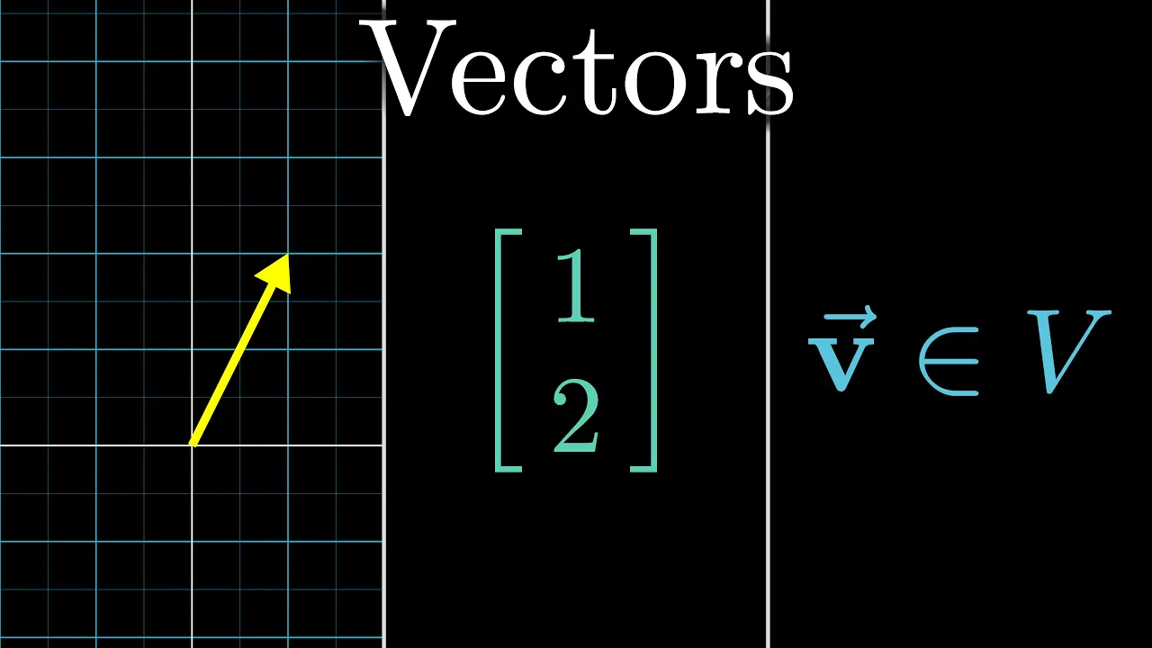
Vectors | Chapter 1, Essence of linear algebra — 3Blue1Brown

3Blue1Brown

Linear algebra derives its analytical power not from geometric arrows or numerical lists alone, but from the ability to translate spatial movements directly into computable arrays.

AI-assisted summary of Vectors | Chapter 1, Essence of linear algebra — original source. Check the original for full context.

Source published:

Key ideas

  • Linear algebra is anchored by three primary perspectives on vectors: arrows in space (physics), ordered lists of numbers (computer science), and generalized algebraic objects (mathematics). (0:00)
  • For geometric visualization in linear algebra, vectors are almost always fixed with their tails at the origin of a coordinate system. (2:04)
  • The entire foundation of linear algebra rests on two core operations: vector addition and scalar multiplication. (4:36)
  • The real power of linear algebra comes from bridging the gap between geometric visual intuition and algorithmic numerical representation. (6:54)

Detailed notes

## Background Published on August 6, 2016, by Grant Sanderson on the YouTube channel 3Blue1Brown, this video serves as the opening chapter of the "Essence of linear algebra" series. According to the video description, the lesson kicks off the playlist by introducing the core basics of vectors through custom visual animations.

## TL;DR Grant Sanderson establishes the vector as the foundational building block of linear algebra, contrasting how it is viewed by physics students (arrows in space), computer science students (ordered lists of numbers), and mathematicians (generalized objects supporting addition and scaling). By rooting vectors at the coordinate origin, numerical coordinates are shown to describe physical movement instructions through space. The lesson details the two primary operations of linear algebra—tip-to-tail vector addition and scalar multiplication—demonstrating how they operate both visually and numerically. Ultimately, Sanderson emphasizes that linear algebra's core power lies in seamlessly translating back and forth between geometric intuition and computational data.

## Atmosphere & style The presentation is marked by 3Blue1Brown's calm, contemplative, and methodically paced delivery, making dense foundational concepts feel accessible and intellectually rewarding. Sanderson's warm, patient voice accompanies clean visual animations, stripping away rote memorization in favor of spatial clarity. Watching the video feels like an intuitive, quiet awakening, where rigid algebraic formulas naturally blossom into fluid, physical movements across a grid.

## Bulletin - [00:00](https://www.youtube.com/watch?v=fNk_zzaMoSs&t=0s) Linear algebra is anchored by three primary perspectives on vectors: arrows in space (physics), ordered lists of numbers (computer science), and generalized algebraic objects (mathematics). - [02:04](https://www.youtube.com/watch?v=fNk_zzaMoSs&t=124s) For geometric visualization in linear algebra, vectors are almost always fixed with their tails at the origin of a coordinate system. - [04:36](https://www.youtube.com/watch?v=fNk_zzaMoSs&t=276s) The entire foundation of linear algebra rests on two core operations: vector addition and scalar multiplication. - [06:54](https://www.youtube.com/watch?v=fNk_zzaMoSs&t=414s) The real power of linear algebra comes from bridging the gap between geometric visual intuition and algorithmic numerical representation.

## Key takeaways - [00:00](https://www.youtube.com/watch?v=fNk_zzaMoSs&t=0s) The fundamental building block for all of linear algebra is the vector. - [00:25](https://www.youtube.com/watch?v=fNk_zzaMoSs&t=25s) In physics, vectors are defined by length and direction and can be translated freely anywhere in space. - [00:55](https://www.youtube.com/watch?v=fNk_zzaMoSs&t=55s) In computer science, vectors are ordered lists of numbers, where list length corresponds to dimensionality. - [01:24](https://www.youtube.com/watch?v=fNk_zzaMoSs&t=84s) In mathematics, vectors are generalized abstract objects that support vector addition and scalar multiplication. - [02:04](https://www.youtube.com/watch?v=fNk_zzaMoSs&t=124s) Unlike in pure physics, linear algebra typically anchors vectors with their tails fixed at the origin of a coordinate system. - [02:38](https://www.youtube.com/watch?v=fNk_zzaMoSs&t=158s) Vector coordinates represent step-by-step movement instructions from the origin to the arrow's tip along each axis. - [03:38](https://www.youtube.com/watch?v=fNk_zzaMoSs&t=218s) Vector coordinates are conventionally written as vertical arrays in square brackets to distinguish them from points. - [04:36](https://www.youtube.com/watch?v=fNk_zzaMoSs&t=276s) Geometric vector addition is performed using the tip-to-tail method, representing sequential spatial displacements. - [05:15](https://www.youtube.com/watch?v=fNk_zzaMoSs&t=315s) Vector addition chaining is virtually the only instance where vectors in linear algebra leave the origin. - [06:12](https://www.youtube.com/watch?v=fNk_zzaMoSs&t=372s) Numerically, adding vectors corresponds to adding their components row-by-row. - [06:54](https://www.youtube.com/watch?v=fNk_zzaMoSs&t=414s) Multiplying a vector by a scalar stretches, squishes, or reverses the arrow's length without changing its underlying line. - [07:35](https://www.youtube.com/watch?v=fNk_zzaMoSs&t=455s) The term 'scalar' originates from the geometric action of scaling a vector, making 'scalar' and 'number' virtually interchangeable. - [08:07](https://www.youtube.com/watch?v=fNk_zzaMoSs&t=487s) Linear algebra's primary utility lies in translating fluidly between spatial geometric intuition and numerical array calculations. - [08:30](https://www.youtube.com/watch?v=fNk_zzaMoSs&t=510s) Data analysts use linear algebra to project numerical datasets into visual geometric spaces to identify patterns. - [08:55](https://www.youtube.com/watch?v=fNk_zzaMoSs&t=535s) Computer graphics and animation engines rely on linear algebra to convert spatial geometric transformations into screen pixel coordinates.

## Detailed walkthrough ### [00:00](https://www.youtube.com/watch?v=fNk_zzaMoSs&t=0s) Three Perspectives on Vectors

Grant Sanderson opens the series by establishing that “the fundamental, root-of-it-all building block for linear algebra is the vector.” Because everything else builds upon this core object, it is essential to clarify what a vector actually is. Broadly speaking, people conceptualize vectors through three distinct yet tightly connected lenses: the physics student perspective, the computer science student perspective, and the mathematician’s perspective.

```mermaid flowchart TD accTitle: Three Perspectives on Vectors accDescr: Diagram illustrating the three distinct lenses of vectors converging into linear algebra. subgraph Perspectives["Three Points of View"] P["Physics: Arrows in Space<br>(Length & Direction)"] CS["Computer Science: Ordered Lists<br>(e.g., [sq ft, price])"] M["Mathematician: Abstract Elements<br>(Vector addition & scalar multiplication)"] end LA["Linear Algebra Foundation"] P --> LA CS --> LA M --> LA ```

To the physics student, vectors are concrete arrows pointing in space, completely characterized by two properties: length and the direction they point. As long as length and direction remain unchanged, you can shift the vector anywhere in space and it remains the exact same vector. Within this framework, vectors lying on a flat plane are two-dimensional, whereas those residing in the physical space we inhabit are three-dimensional.

In contrast, the computer science student views vectors as ordered lists of numbers. If an analyst were tracking house prices using only square footage and price, each house could be modeled as a pair of numbers where the first value indicates square footage and the second represents price. Order is critical here, because swapping the numbers fundamentally changes their meaning. In that domain, vector serves merely as a fancy term for a list, and the list’s dimension simply corresponds to its length.

The mathematician aims to generalize both viewpoints, asserting that a vector can be essentially anything for which sensible notions of vector addition and scalar multiplication exist. While Sanderson notes that this abstract view is best set aside until the final video of the series in favor of more concrete intuition, its existence highlights why those two specific operations form the bedrock of linear algebra.

- **Physics perspective**: Arrows with length and direction; translation-invariant (can sit anywhere in space). - **Computer science perspective**: Ordered lists of numbers; list length equals dimensionality. - **Mathematician perspective**: Generalized objects supporting vector addition and multiplication by a number.

---

[02:04](https://www.youtube.com/watch?v=fNk_zzaMoSs&t=124s) The Geometric Foundation and Coordinate Systems

For the visual, geometric focus of this series, Sanderson advises starting with a specific mental image: an arrow situated inside a coordinate system—such as the standard $xy$-plane—anchored with its tail fixed directly at the origin. This departs slightly from pure physics intuition: “In linear algebra, it's almost always the case that your vector will be rooted at the origin.” Once an intuition is established via arrows in space, it translates immediately into the list-of-numbers perspective by using vector coordinates.

In a two-dimensional system, space is structured around a horizontal $x$-axis and a vertical $y$-axis intersecting at the origin, which functions as the center of space and the root of every vector. After establishing an arbitrary unit length denoted by tick marks (which can be expanded into grid lines to visualize space as a whole), coordinates describe a set of movement instructions from the tail at the origin to the arrow's tip: 1. The first number gives the distance to travel along the $x$-axis (positive values indicate rightward motion; negative values indicate leftward motion). 2. The second number indicates how far to walk parallel to the $y$-axis (positive values denote upward movement; negative values denote downward movement).

``` y-axis ^ | * tip: [x, y] | / | / | / vector arrow | / | / -----+---*-----------------> x-axis | origin [0, 0] | ```

To distinguish vectors from standard geometric points, convention dictates writing the coordinate pair vertically inside square brackets: $$\begin{bmatrix} x \\ y \end{bmatrix}$$ Every pair of numbers defines a unique vector, and every vector is paired with exactly one set of coordinates. In three dimensions, this logic extends naturally by introducing a $z$-axis perpendicular to both the $x$ and $y$-axes. Each 3D vector corresponds to a unique ordered triplet of numbers, dictating motion along $x$, then parallel to $y$, and finally parallel to the $z$-axis.

---

[04:36](https://www.youtube.com/watch?v=fNk_zzaMoSs&t=276s) Vector Addition: Tip-to-Tail and Movement

Linear algebra continuously returns to two core operations: vector addition and scalar multiplication. Geometrically, vector addition follows the tip-to-tail method. If you take two vectors—say, one directed up and slightly right, and another pointing down and to the right—you compute their sum by moving the second vector so that its tail connects directly to the tip of the first. Drawing a new arrow starting at the tail of the first vector and extending to the tip of the second produces their vector sum.

``` /| (tip of v1) / | / | v1 / | v2 / v / \ *--------> (tip of v2) tail of v1 [===================>] Sum: v1 + v2 ```

Sanderson points out that this chaining process represents virtually the only moment in linear algebra where vectors are permitted to leave the origin. The intuition behind this construction comes down to treating vectors as physical displacements: “The way I like to think about it is that each vector represents a certain movement, a step with a certain distance and direction in space.” Applying the second step after completing the first yields the exact same total displacement as traversing the direct sum vector from the start. This directly generalizes standard elementary arithmetic: adding $2 + 5$ on a number line involves walking two steps right, then another five steps right, landing at seven.

Numerically, this behavior translates to simple component-wise arithmetic. For a vector with coordinates $\begin{bmatrix} 1 \\ 2 \end{bmatrix}$ added to a vector $\begin{bmatrix} 3 \\ -1 \end{bmatrix}$: - Walk $1$ unit right, then $2$ units up. - Then walk $3$ units right, and $1$ unit down.

Grouping the horizontal motion together and the vertical motion together produces: $$\begin{bmatrix} 1 \\ 2 \end{bmatrix} + \begin{bmatrix} 3 \\ -1 \end{bmatrix} = \begin{bmatrix} 1 + 3 \\ 2 + (-1) \end{bmatrix} = \begin{bmatrix} 4 \\ 1 \end{bmatrix}$$ In general, adding vectors in the list-of-numbers view simply means pairing up corresponding entries and computing their sums.

---

[06:54](https://www.youtube.com/watch?v=fNk_zzaMoSs&t=414s) Scalar Multiplication and the Bridge Between Perspectives

The second fundamental operation is multiplying a vector by a number. Geometrically, this alters the vector's length without changing its underlying line of action: - Multiplying a vector by $2$ doubles its length, stretching it outward. - Multiplying by $\frac{1}{3}$ squishes the vector down to one-third of its initial size. - Multiplying by a negative factor like $-1.8$ flips the vector’s direction $180^\circ$ and scales its length by $1.8$.

``` Original vector: --------> Multiplied by 2: ----------------> Multiplied by 1/3: --> Multiplied by -1: <-------- ```

This act of stretching, squishing, or flipping direction is termed **scaling**, and any number performing this role is called a **scalar**. In linear algebra, numbers primarily act to scale vectors, making the words "number" and "scalar" practically interchangeable. Computationally, scaling an arrow corresponds directly to scaling each of its components: multiplying a vector by $2$ doubles both its $x$ and $y$ values.

Sanderson reflects on the broader value of these mechanics, noting that the true power of the discipline lies not in crowning one representation superior to the other, but in mastering the movement between them: > “The usefulness of linear algebra has less to do with either one of these views than it does with the ability to translate back and forth between them.”

This two-way bridge serves distinct disciplines: - **Data analysts** take lists of numerical data and project them geometrically, making complex patterns visible and granting a high-level intuition for how data transformations behave. - **Physicists and computer graphics programmers** take geometric ideas about physical space and translate them into lists of numbers that computers can process algorithmically.

Sanderson notes that his own mathematical animations rely on this exact bridge: he visualizes geometric transformations in space and relies on linear algebra to convert those movements into raw coordinate numbers that tell the computer where to place pixels on the screen. The video wraps up by previewing the upcoming concepts that build directly on these foundations: span, bases, and linear dependence.

## Notable quotes > [04:36](https://www.youtube.com/watch?v=fNk_zzaMoSs&t=276s) The way I like to think about it is that each vector represents a certain movement, a step with a certain distance and direction in space. — Grant Sanderson

> [02:04](https://www.youtube.com/watch?v=fNk_zzaMoSs&t=124s) In linear algebra, it's almost always the case that your vector will be rooted at the origin. — Grant Sanderson

> [00:00](https://www.youtube.com/watch?v=fNk_zzaMoSs&t=0s) the fundamental, root-of-it-all building block for linear algebra is the vector. — Grant Sanderson

## Mentioned 3Blue1Brown, Grant Sanderson, Essence of linear algebra, Vince Rubinetti, HTW Berlin

## Video description Beginning the linear algebra series with the basics. Help fund future projects: https://www.patreon.com/3blue1brown

Music: https://vincerubinetti.bandcamp.com/track/grants-etude

Thanks to Elo Marie Viennot and Ambros Gleixner from HTW Berlin (www.htw-berlin.de) for contributing German translations and dubbing.

Thanks also to these viewers for their contributions to the subtitles Arabic: @Cewkins, Hazem Bengali: Md Rasheduzzaman Czech: @Chnapak Greek: Nikolaos Tsagkas Hebrew: Omer Tuchfeld Italian: mattiacolucci Spanish: Juan Carlos Largo Thai: own doggoV●ᴥ●V

------------------

3blue1brown is a channel about animating math, in all senses of the word animate. And you know the drill with YouTube, if you want to stay posted about new videos, subscribe, and click the bell to receive notifications (if you're into that).

If you are new to this channel and want to see more, a good place to start is this playlist: https://goo.gl/WmnCQZ

Various social media stuffs: Website: https://www.3blue1brown.com Twitter: https://twitter.com/3Blue1Brown Patreon: https://patreon.com/3blue1brown Facebook: https://www.facebook.com/3blue1brown Reddit: https://www.reddit.com/r/3Blue1Brown

[Source](https://www.youtube.com/watch?v=fNk_zzaMoSs)

中文简报

桑德森以原点向量为基石统合数学与编程 线性代数的分析能力并非仅源于几何箭头或数字列表,而是源于将空间运动直接转化为可计算数组的能力。 格兰特·桑德森将向量确立为线性代数的基础构件,并对比了物理系学生(空间中的箭头)、计算机科学系学生(有序数字列表)和数学家(支持加法与数乘的广义对象)对它的不同视角。通过将向量固定在坐标原点,数值坐标被展现为描述在空间中移动的物理指令。本课详细阐述了线性代数的两大核心运算——首尾相连的向量加法与标量乘法,展示了它们在视觉和数值上的运作方式。最终,桑德森强调,线性代数的核心威力在于能够在几何直觉与计算数据之间进行无缝的双向转换。 线性代数立足于对向量的三种主要视角:空间中的箭头(物理学)、有序数字列表(计算机科学)以及广义代数对象(数学)。 (0:00) 在线性代数的几何可视化中,向量的起点几乎总是固定在坐标系的原点。 (2:04) 线性代数的整个基础建立在两大核心运算之上:向量加法与标量乘法。 (4:36) 线性代数的真正威力源于弥合几何视觉直觉与算法数值表示之间的差距。 (6:54)

Reading summary

Grant Sanderson establishes the vector as the foundational building block of linear algebra, arguing that the discipline's primary strength lies in translating fluidly between geometric arrows and numerical data lists. Three Core Perspectives on Vectors (0:00) Sanderson identifies three primary lenses through which vectors are understood. In physics, vectors are translation-invariant arrows possessing length and direction that can reside anywhere in space. In computer science, vectors are ordered lists of numbers where list length dictates dimensionality, such as pairing square footage and price to model real estate. Mathematicians generalize both views, defining vectors as any objects for which vector addition and scalar multiplication are valid operations. Coordinate Systems and Origin Anchoring (2:04) For geometric intuition, linear algebra departs from physics by anchoring the tail of a vector at the coordinate origin. Coordinates written vertically, such as an x-component over a y-component inside square brackets, represent directional walking instructions from the origin to the arrow's tip along each axis. This framework pairs every coordinate tuple with a unique arrow in space and extends directly to three dimensions by introducing an orthogonal z-axis. Vector Addition as Sequential Displacement (4:36) Geometrically, adding vectors follows the tip-to-tail rule, chaining arrows together to represent consecutive movements or displacements through space. Sanderson notes that this chaining represents virtually the only instance where vectors leave the origin. Computationally, this sequential motion directly corresponds to component-wise addition, where corresponding entries are summed independently, such as adding the vectors [1, 2] and [3, -1] to yield [4, 1]. Scaling Vectors Across the Conceptual Bridge (6:54) Multiplying a vector by a scalar changes its length by stretching, squishing, or reversing its direction by 180 degrees if the scalar is negative. Computationally, this scales each coordinate entry by that factor. Sanderson emphasizes that the practical utility of linear algebra lies in moving between representations: data analysts translate numerical datasets into geometric spaces to uncover patterns, while physicists and computer graphics programmers convert spatial transformations into coordinate arrays for algorithmic computation. Sanderson defers the mathematician's fully abstract view of vectors to later in the series, maintaining that anchoring concrete geometric intuitions to coordinate arithmetic forms the prerequisite foundation for understanding concepts like span, bases, and linear dependence.

精炼阅读摘要

Grant Sanderson 指出,向量是线性代数的根本基石;理解该学科的关键不在于孤立看待几何图形或数值列表,而在于建立空间中的“几何箭头”与计算机中的“有序数字列表”之间自由互译的能力。 向量定义的三种视角与抽象统一 (0:00) 不同学科对向量的定义呈现出三种紧密相连的视角。在物理学视角下,向量是具有特定长度和方向的空间箭头,具有平移不变性,即只要长度与方向保持不变,向量在空间中处于任何位置都被视为同一个对象;在计算机科学视角下,向量是有序的数字列表,例如用面积和价格两个数值建模房屋数据,数值的排列顺序不可颠倒,列表长度即对应向量的维度。数学家则对这两种视角进行了抽象推广,认为只要对特定对象定义了合理的向量加法与标量乘法,该对象即可被视为向量。这种抽象视角印证了加法和数乘是支撑线性代数大厦的两大底层运算。 坐标系统与固定原点的几何锚定 (2:04) 在线性代数的几何直觉中,向量几乎总是以坐标系的原点为唯一起点,这与纯物理中可自由平移的箭头略有不同。在二维坐标系中,空间由互相垂直的 x 轴和 y 轴界定,原点既是空间的中心,也是所有向量的尾部锚点。坐标系中设定的单位刻度与扩展网格,为量化向量提供了度量基础。在书写规范上,线性代数习惯将数值对垂直排列在方括号内,以此区分几何点与向量。这对数字实质上是从原点移动至箭头尖端的“行动指南”:第一个数字指示沿 x 轴的移动距离(正数向右,负数向左),第二个数字指示平行于 y 轴的移动距离(正数向上,负数向下)。这种一一对应关系确保了每对坐标唯一确定一个向量,该逻辑也能自然推广至包含 z 轴的三维空间。 向量加法:位移累加与分量求和 (4:36) 几何层面的向量加法遵循“首尾相连法”(Tip-to-Tail)。计算两个向量相加时,将第二个向量的尾部平移对接至第一个向量的尖端,从初始尾部连接到末端尖端的新箭头即为两者的和向量。这是线性代数中极少数允许向量暂时离开原点的场景。Sanderson 指出,这种操作的直观内核在于将向量视为物理“位移”:相继执行两次位移所达到的最终空间位置,与直接沿和向量单次位移的效果完全相同,这直接推广了一维数轴上基础算术的加法逻辑。在代数层面,这一几何行为精确对应于各分量的逐项相加。例如将沿 x 轴位移 1、y 轴位移 2 的向量与位移为 3 和 -1 的向量相加,最终水平总位移为 1 加 3 等于 4,垂直总位移为 2 加 -1 等于 1。列表视角下的分量相加正是几何空间位移叠加的直接体现。 标量数乘与跨学科的双向转换桥梁 (6:54) 线性代数的第二项基本运算是数乘,即用一个数字乘以向量。在几何上,这表现为在不改变向量所在直线的前提下拉伸、压缩或翻转箭头:乘以大于 1 的正数会同向拉长向量,乘以小于 1 的正数会缩短向量,而乘以负数则会使箭头反向翻转 180 度。因为数字在此过程中扮演了缩放向量的角色,线性代数通常将数字统称为“标量”(Scalar),在计算中对应于将每个坐标分量均乘以该标量数值。Sanderson 强调,线性代数的真正威力正是充当了连接几何与代数的双向桥梁:数据分析师能将抽象的高维数字列表投射为空间几何图形,以便观察复杂数据模式与变换;物理学家和计算机图形学开发者则能把物理空间的几何变换翻译成可供计算机执行算法的具体坐标数值。 Sanderson 总结指出,向量的坐标表示、首尾相连的加法以及标量缩放构成了整套理论的地基,熟练掌握几何与代数视角的相互转换,是后续理解张成空间(Span)、基底(Bases)和线性相关性(Linear Dependence)等核心概念的前提。

Detailed notes — zh

## Background 本内容由知名数学科普频道 3Blue1Brown 于 2016 年 8 月 6 日发布在 YouTube 平台上。视频是其备受赞誉的《线性代数的本质》(Essence of linear algebra)系列第一章,旨在从最基础的基石概念——向量——出发,开启对线性代数的直观几何探索。 ## TL;DR 视频首先对比了物理学(自由箭头)、计算机科学(有序数字列表)与数学(满足公理的抽象对象)三种不同的向量视角,并确立了本系列以原点为起点的几何坐标体系。随后,Grant 详细拆解了线性代数的两大核心基石运算:几何上通过首尾相接、代数上通过分量对应相加的“向量加法”,以及代表拉伸、压缩与反转的“标量乘法”。最后强调,线性代数真正的魅力与威力,正是在于连接抽象数字列表与直观空间几何之间的双向互译能力。 ## Atmosphere & style 整期视频散发着 3Blue1Brown 标志性的从容、优雅与启发性,配乐宁静优美,极具沉浸感。Grant Sanderson 语调温和清晰,像一位耐心的向导,将枯燥的公式化教学拆解为生动直观的空间动态。观看体验极其愉悦,让原本抽象甚至令人头疼的代数符号在眼前瞬间变得具象而鲜活,带来一种豁然开朗的智力美感。 ## Bulletin - [00:00](https://www.youtube.com/watch?v=fNk_zzaMoSs&t=0s) 向量是线性代数最根本的基石,主要存在物理学(带方向与长度的箭头)、计算机科学(有序数字列表)与数学家(满足加法与数乘公理的抽象对象)三种核心视角。 - [02:04](https://www.youtube.com/watch?v=fNk_zzaMoSs&t=124s) 在几何直觉建立过程中,线性代数通常将向量的起点固定在原点,并将坐标分量理解为从原点到达箭头尖端的移动指令。 - [04:36](https://www.youtube.com/watch?v=fNk_zzaMoSs&t=276s) 向量加法(首尾相接对应位移累加)与标量乘法(对向量进行拉伸、压缩或反转的缩放操作)构成了整个线性代数体系运转的基础运算。 - [08:10](https://www.youtube.com/watch?v=fNk_zzaMoSs&t=490s) 线性代数的核心价值在于架起几何空间与数值计算之间的“双向互译”桥梁,既可为数据分析提供几何直觉,也能将空间变换转化为计算机可处理的数组。 ## Key takeaways - [00:00](https://www.youtube.com/watch?v=fNk_zzaMoSs&t=0s) 向量是线性代数的根本构建基石,不同领域对其理解各异但相通。 - [00:00](https://www.youtube.com/watch?v=fNk_zzaMoSs&t=0s) 物理学视角将向量定义为具有长度和方向的空间箭头,其在空间中自由平移时不改变向量本身。 - [00:00](https://www.youtube.com/watch?v=fNk_zzaMoSs&t=0s) 计算机科学视角将向量视为有序的数字列表,列表长度直接对应向量的维度(如房产面积与价格构成的二维向量)。 - [00:00](https://www.youtube.com/watch?v=fNk_zzaMoSs&t=0s) 数学家视角对向量进行了终极抽象,只要某种对象定义了合理的相加与数乘规则,即可被称为向量。 - [02:04](https://www.youtube.com/watch?v=fNk_zzaMoSs&t=124s) 为了建立几何直觉,线性代数通常约定将向量的尾端固定在坐标系的原点,以此区别于物理学中的自由平移箭头。 - [02:04](https://www.youtube.com/watch?v=fNk_zzaMoSs&t=124s) 向量的列坐标是一套明确的位移指南,指示从原点出发分别沿各坐标轴行进的距离与方向。 - [04:36](https://www.youtube.com/watch?v=fNk_zzaMoSs&t=276s) 在几何上,向量加法通过将第二个向量首尾相接在第一个向量末端来定义,代表两次连续空间位移的合成效果。 - [04:36](https://www.youtube.com/watch?v=fNk_zzaMoSs&t=276s) 向量加法的首尾相接法,是线性代数中极少数允许向量暂时离开原点的情况之一。 - [04:36](https://www.youtube.com/watch?v=fNk_zzaMoSs&t=276s) 向量相加在数值上表现为各维度坐标分量的逐项直接相加,几何位移与代数求和完全契合。 - [06:54](https://www.youtube.com/watch?v=fNk_zzaMoSs&t=414s) 向量与数字相乘的本质是几何上的“缩放”(Scaling),正数改变长度,负数引入 180 度反转,因此线性代数中常将“数字”通称为“标量”。 - [06:54](https://www.youtube.com/watch?v=fNk_zzaMoSs&t=414s) 标量乘法在数值计算上等价于将该标量依次乘以向量的每一个坐标分量。 - [08:10](https://www.youtube.com/watch?v=fNk_zzaMoSs&t=490s) 线性代数的威力在于打通空间与数字的双向通道:将连续空间变换转化为离散数字计算,同时赋予干燥数据直观的几何图像。 ## Detailed walkthrough ### [00:00](https://www.youtube.com/watch?v=fNk_zzaMoSs&t=0s) 向量的三种视角:物理、计算机与数学 作为线性代数最根本、最基石的概念,向量(Vector)在不同学科背景的人眼中有着完全不同的样貌。Grant Sanderson 指出:“The fundamental, root-of-it-all building block for linear algebra is the vector.”(线性代数最基本、最根源的构建基石就是向量。)为了让所有人建立统一的认知,他梳理了三种截然不同却又紧密相关的向量视角: 首先是**物理学学生的视角**:向量是空间中带有指向的箭头。定义一个向量的关键要素是它的“长度”(length)和“所指方向”(direction)。只要这两者保持不变,你就可以在空间中随意平移它,它依然代表同一个向量。平面上的向量是二维的,而真实生活空间中的向量则是三维的。 其次是**计算机科学学生的视角**:向量是“有序的数字列表”(ordered lists of numbers)。例如在做房价数据分析时,如果你只关心房屋的面积和价格,就可以用一对数字来建模每套房子,第一个数字代表面积,第二个数字代表价格。这里的顺序至关重要。在此语境下,“向量”基本上就是列表(list)的高级说法,而列表包含两个数字,就构成了“二维向量”。 最后是**数学家的视角**:数学家试图将上述两种观点泛化。数学家认为,只要某种对象之间存在合理的“相加”(addition)以及“与数相乘”(scalar multiplication)的概念,它就可以被称作向量。Grant Sanderson 坦言这个视角极为抽象,在系列视频的最后一集之前最好先将其搁置,先关注具象内容;但这也预示着向量加法和数乘在线性代数中贯穿始终的核心地位。 ```mermaid flowchart TD accTitle: 三种向量视角的比较与统一 accDescr: 展示物理、计算机与数学三种视角的差异及它们在线性代数中的统一。 subgraph Perspectives["三种视角"] P["物理学视角<br/>空间中的箭头<br/>(长度与方向,可自由平移)"] CS["计算机科学视角<br/>有序数字列表<br/>(如 [面积, 价格])"] M["数学家视角<br/>抽象代数对象<br/>(满足加法与数乘公理)"] end subgraph Core["线性代数核心关注"] G["几何视角:以原点为起点的箭头"] N["数值视角:坐标分量列表"] end P --> G CS --> N M -.->|"抽象推广"| Core G <-->|"坐标映射"| N ``` - **物理学视角**:关注几何特征(长度、方向),与位置无关。 - **计算机科学视角**:关注数据组织,维度即列表长度(如长度为 2 的数字列表即二维向量)。 - **数学家视角**:不关注具体表现形式,只关注运算规则是否满足加法与数乘公理。 --- ### [02:04](https://www.youtube.com/watch?v=fNk_zzaMoSs&t=124s) 线性代数的约定:以原点为起点的坐标体系 由于本系列视频侧重于几何直觉,Grant Sanderson 建议观众在听到“向量”一词时,首先联想到的应当是**坐标系(例如 xy 平面)中以原点为起点的箭头**。这与物理学中允许箭头满空间随意漂移的视角有所不同:在线性代数中,绝大多数情况下向量的尾端都是固定在原点(Origin)上的。只有先在空间箭头语境下理解概念,再将其翻译为数字列表,才能打通几何与代数之间的通路。 在二维坐标系中,水平方向为 x 轴,垂直方向为 y 轴,两轴交点即为原点——也是整个空间的中心与所有向量的根基。在选定单位长度并在坐标轴上标记刻度后,向量的坐标实际上就是**一套从原点移动到箭头尖端的“行动指南”**: - 第一个数字指示沿 x 轴行进的距离(正数向右,负数向左); - 第二个数字指示随后沿平行于 y 轴方向行进的距离(正数向上,负数向下)。 为了在书写上区分“向量”与“点”,标准的线性代数记法是将这组数字垂直排列,并用方括号包裹(即列向量形式)。二维中每个数对唯一对应一个空间向量,每个向量也唯一对应一个数对。同理,推广到三维空间时,只需要引入一条与 x、y 轴皆垂直的 z 轴,三维向量便对应一个三元有序数组,分别指导沿 x 轴、平行 y 轴和平行 z 轴的位移。 --- ### [04:36](https://www.youtube.com/watch?v=fNk_zzaMoSs&t=276s) 向量加法:从首尾相连到代数求和 线性代数的全部理论几乎都是围绕着“向量加法”和“标量乘法”这两个基本运算展开的。从几何上看,两个向量相加有着极为直观的定义:假设有两个向量,一个指向上方略偏右,另一个指向右下方。将第二个向量平移,使其尾端落在第一个向量的尖端,然后从第一个向量的尾端(原点)连接到第二个向量尖端画出一条新向量,这个新向量就是它们的和。Grant Sanderson 特别指出:“This definition of addition, by the way, is pretty much the only time in linear algebra where we let vectors stray away from the origin.”(顺便提一句,这种加法定义几乎是线性代数中唯一允许向量离开原点的情况。) 之所以采用这种“首尾相接”的加法法则,是因为每个向量本质上代表着空间中的一种“位移步长”(movement)。沿着第一个向量迈出一步,接着再沿着第二个向量的距离与方向迈出第二步,其总体累积位移效果与直接沿着合向量走完全一致。这就像小学数学在数轴上教 2 + 5 一样:先向右走 2 步,再向右走 5 步,总效果等于向右走 7 步。 在数值计算上,这一过程同样契合得非常完美。假设第一个向量坐标为 $\begin{bmatrix} 1 \\ 2 \end{bmatrix}$,第二个向量坐标为 $\begin{bmatrix} 3 \\ -1 \end{bmatrix}$: 1. 几何路径是:向右走 1,向上走 2,再向右走 3,向下走 1; 2. 重新整理顺序(先横后纵):向右移动 $(1 + 3)$,随后垂直移动 $(2 - 1)$; 3. 最终得到新向量坐标为 $\begin{bmatrix} 1 + 3 \\ 2 + (-1) \end{bmatrix} = \begin{bmatrix} 4 \\ 1 \end{bmatrix}$。 在数字列表的视角下,向量加法就是将对应位置上的分量逐一相加。 --- ### [06:54](https://www.youtube.com/watch?v=fNk_zzaMoSs&t=414s) 标量乘法与“缩放”概念 第二个基石运算是向量与数字相乘。理解这一运算的最佳方式是观察其实际作用: - 将向量乘以 2,意味着将其长度拉伸为原本的 2 倍; - 将向量乘以 1/3,意味着将其压缩至原始长度的三分之一; - 将向量乘以负数(例如 -1.8),向量会先经历 180 度反向(flip around),然后再拉伸至 1.8 倍长。 这种拉伸、压缩或反转向量方向的过程被称为**缩放**(Scaling)。在这个过程中发挥作用的数字(如 2、1/3 或 -1.8)就被称为**标量**(Scalar)。Grant Sanderson 解释道:“In fact, throughout linear algebra, one of the main things that numbers do is scale vectors, so it's common to use the word scalar pretty much interchangeably with the word number.”(事实上,贯穿整个线性代数,数字最主要的作用之一就是缩放向量,因此在很多时候,‘标量’和‘数字’这两个词几乎是完全通用的。) 在数值层面,将几何向量拉伸 2 倍,等价于将其每一个坐标分量都乘以 2。因此在列表视角中,数乘向量即是将标量依次乘到每一个分量上。 --- ### [08:10](https://www.youtube.com/watch?v=fNk_zzaMoSs&t=490s) 空间与数字的双向互译 在线性代数中,无论你认为向量本质上是“碰巧能用数字表示的空间箭头”,还是“碰巧拥有几何意义的数字列表”,都无关紧要。这门学科真正的威力在于能够在两者之间自如地进行“双向互译”: - **对于数据分析师**:线性代数提供了一种将大量枯燥数字列表进行视觉化、几何化构想的途径,能够清晰呈现数据模式,并从全局角度洞察特定运算的本质; - **对于物理学家和计算机图形学开发者**:线性代数则提供了一套将连续空间以及空间的变换动作,精确翻译为可供计算机高效运算与处理的纯数字语言。 Grant Sanderson 以自己的数学动画创作为例说明:他制作动画时,总是先在大脑中构思空间里正在发生什么几何运动,再通过计算机的数值计算确定屏幕上每个像素应当落下的位置,而这一整套流程完全依托于扎实的线性代数认知。在建立起向量加法与标量乘法这两个基础工具后,后续视频将进一步探索线性代数中更迷人的核心概念,如张成空间(Span)、基(Basis)以及线性相关性(Linear Dependence)。 ## Notable quotes > [00:00](https://www.youtube.com/watch?v=fNk_zzaMoSs&t=0s) The fundamental, root-of-it-all building block for linear algebra is the vector. — Grant Sanderson > [06:54](https://www.youtube.com/watch?v=fNk_zzaMoSs&t=414s) In fact, throughout linear algebra, one of the main things that numbers do is scale vectors, so it's common to use the word scalar pretty much interchangeably with the word number. — Grant Sanderson ## Mentioned Grant Sanderson, 3Blue1Brown, 线性代数, HTW Berlin ## Video description Beginning the linear algebra series with the basics. Help fund future projects: https://www.patreon.com/3blue1brown Music: https://vincerubinetti.bandcamp.com/track/grants-etude Thanks to Elo Marie Viennot and Ambros Gleixner from HTW Berlin (www.htw-berlin.de) for contributing German translations and dubbing. Thanks also to these viewers for their contributions to the subtitles Arabic: @Cewkins, Hazem Bengali: Md Rasheduzzaman Czech: @Chnapak Greek: Nikolaos Tsagkas Hebrew: Omer Tuchfeld Italian: mattiacolucci Spanish: Juan Carlos Largo Thai: own doggoV●ᴥ●V ------------------ 3blue1brown is a channel about animating math, in all senses of the word animate. And you know the drill with YouTube, if you want to stay posted about new videos, subscribe, and click the bell to receive notifications (if you're into that). If you are new to this channel and want to see more, a good place to start is this playlist: https://goo.gl/WmnCQZ Various social media stuffs: Website: https://www.3blue1brown.com Twitter: https://twitter.com/3Blue1Brown Patreon: https://patreon.com/3blue1brown Facebook: https://www.facebook.com/3blue1brown Reddit: https://www.reddit.com/r/3Blue1Brown [Source](https://www.youtube.com/watch?v=fNk_zzaMoSs)

Source quotes

[0:00] Grant Sanderson: The fundamental, root-of-it-all building block for linear algebra is the vector. [6:54] Grant Sanderson: In fact, throughout linear algebra, one of the main things that numbers do is scale vectors, so it's common to use the word scalar pretty much interchangeably with the word number.

Source quotes

[4:36] Grant Sanderson: The way I like to think about it is that each vector represents a certain movement, a step with a certain distance and direction in space. [2:04] Grant Sanderson: In linear algebra, it's almost always the case that your vector will be rooted at the origin. [0:00] Grant Sanderson: the fundamental, root-of-it-all building block for linear algebra is the vector.

Original transcript

[0:00] [Translated by Grant Sanderson. Submit corrections at criblate.com] [0:10] The fundamental, root-of-it-all building block for linear algebra is the vector. [0:15] So it's worth making sure that we're all on the same page about what exactly a vector is. [0:20] You see, broadly speaking, there are three distinct but related ideas about vectors, [0:24] which I'll call the physics student perspective, [0:26] the computer science student perspective, and the mathematician's perspective. [0:30] The physics student perspective is that vectors are arrows pointing in space. [0:34] What defines a given vector is its length and the direction it's pointing, [0:38] but as long as those two facts are the same, you can move it all around, [0:41] and it's still the same vector. [0:44] Vectors that live in the flat plane are two-dimensional, [0:46] and those sitting in broader space that you and I live in are three-dimensional. [0:51] The computer science perspective is that vectors are ordered lists of numbers. [0:55] For example, let's say you were doing some analytics about house prices, [0:59] and the only features you cared about were square footage and price. [1:03] You might model each house with a pair of numbers, [1:05] the first indicating square footage and the second indicating price. [1:09] Notice the order matters here. [1:12] In the lingo, you'd be modeling houses as two-dimensional vectors, [1:15] where in this context, vector is pretty much just a fancy word for list, [1:19] and what makes it two-dimensional is the fact that the length of that list is two. [1:25] The mathematician, on the other hand, seeks to generalize both these views, [1:29] basically saying that a vector can be anything where there's a sensible notion of adding [1:33] two vectors and multiplying a vector by a number, [1:36] operations that I'll talk about later on in this video. [1:39] The details of this view are rather abstract, and I actually think it's healthy to ignore [1:43] it until the last video of this series, favoring a more concrete setting in the interim. [1:48] But the reason I bring it up here is that it hints at the fact [1:51] that the ideas of vector addition and multiplication by [1:54] numbers will play an important role throughout linear algebra. [1:58] But before I talk about those operations, let's just settle in on [2:01] a specific thought to have in mind when I say the word vector. [2:04] Given the geometric focus that I'm shooting for here, [2:07] whenever I introduce a new topic involving vectors, [2:10] I want you to first think about an arrow, and specifically, [2:13] think about that arrow inside a coordinate system, like the xy-plane, [2:16] with its tail sitting at the origin. [2:19] This is a little bit different from the physics student perspective, [2:22] where vectors can freely sit anywhere they want in space. [2:25] In linear algebra, it's almost always the case [2:27] that your vector will be rooted at the origin. [2:30] Then, once you understand a new concept in the context of arrows in space, [2:34] we'll translate it over to the list of numbers point of view, [2:37] which we can do by considering the coordinates of the vector. [2:41] Now, while I'm sure that many of you are already familiar with this coordinate system, [2:45] it's worth walking through explicitly, since this is where all of the important [2:48] back and forth happens between the two perspectives of linear algebra. [2:52] Focusing our attention on two dimensions for the moment, you have a horizontal line, [2:56] called the x-axis, and a vertical line, called the y-axis. [3:00] The place where they intersect is called the origin, [3:02] which you should think of as the center of space and the root of all vectors. [3:06] After choosing an arbitrary length to represent one, [3:08] you make tick marks on each axis to represent this distance. [3:12] When I want to convey the idea of 2D space as a whole, [3:14] which you'll see comes up a lot in these videos, [3:16] I'll extend these tick marks to make grid lines, but right now, [3:19] they'll actually get a little bit in the way. [3:22] The coordinates of a vector is a pair of numbers that basically gives instructions [3:26] for how to get from the tail of that vector at the origin to its tip. [3:30] The first number tells you how far to walk along the x-axis, [3:33] positive numbers indicating rightward motion, [3:36] negative numbers indicating leftward motion, and the second number tells you how [3:40] far to walk parallel to the y-axis after that, [3:42] positive numbers indicating upward motion, and negative numbers indicating downward [3:47] motion. [3:48] To distinguish vectors from points, the convention is to write [3:51] this pair of numbers vertically with square brackets around them. [3:56] Every pair of numbers gives you one and only one vector, [3:59] and every vector is associated with one and only one pair of numbers. [4:04] What about in three dimensions? [4:06] Well, you add a third axis, called the z-axis, [4:08] which is perpendicular to both the x and y-axes, and in this case, [4:12] each vector is associated with ordered triplet of numbers. [4:16] The first tells you how far to move along the x-axis, [4:19] the second tells you how far to move parallel to the y-axis, [4:23] and the third one tells you how far to then move parallel to this new z-axis. [4:28] Every triplet of numbers gives you one unique vector in space, [4:31] and every vector in space gives you exactly one triplet of numbers. [4:36] All right, so back to vector addition and multiplication by numbers. [4:40] After all, every topic in linear algebra is going to center around these two operations. [4:45] Luckily, each one's pretty straightforward to define. [4:48] Let's say we have two vectors, one pointing up and a little to the right, [4:51] and the other one pointing right and down a bit. [4:53] To add these two vectors, move the second one so [4:56] that its tail sits at the tip of the first one. [5:00] Then, if you draw a new vector from the tail of the first one to [5:04] where the tip of the second one sits, that new vector is their sum. [5:12] This definition of addition, by the way, is pretty much the only time [5:15] in linear algebra where we let vectors stray away from the origin. [5:19] Now, why is this a reasonable thing to do? [5:21] Why this definition of addition and not some other one? [5:25] Well, the way I like to think about it is that each vector represents a certain movement, [5:29] a step with a certain distance and direction in space. [5:33] If you take a step along the first vector, then take a step in the direction [5:37] and distance described by the second vector, the overall effect is just [5:41] the same as if you moved along the sum of those two vectors to start with. [5:45] You could think about this as an extension of how [5:47] we think about adding numbers on a number line. [5:50] One way that we teach kids to think about this, say with 2 plus 5, [5:53] is to think of moving two steps to the right followed by another five steps to the right. [5:57] The overall effect is the same as if you just took seven steps to the right. [6:02] In fact, let's see how vector addition looks numerically. [6:06] The first vector here has coordinates 1, 2, and the second one has coordinates 3, [6:11] negative 1. [6:14] When you take the vector sum using this tip-to-tail method, [6:17] you can think of a four-step path from the origin to the tip of the second vector. [6:21] Walk 1 to the right, then 2 up, then 3 to the right, then 1 down. [6:26] Reorganizing these steps so that you first do all of the rightward motion, [6:31] then do all the vertical motion, you can read it as saying first [6:35] move 1 plus 3 to the right, then move 2 minus 1 up. [6:40] So the new vector has coordinates 1 plus 3 and 2 plus negative 1. [6:45] In general, vector addition in this list of numbers conception [6:49] looks like matching up their terms and adding each one together. [6:54] The other fundamental vector operation is multiplication by a number. [6:58] Now this is best understood just by looking at a few examples. [7:01] If you take the number 2 and multiply it by a given vector, [7:04] it means you stretch out that vector so that it's two times as long as when you started. [7:10] If you multiply that vector by, say, one-third, [7:13] it means you squish it down so that it's one-third the original length. [7:17] When you multiply it by a negative number, like negative 1.8, [7:21] then the vector first gets flipped around, then stretched out by that factor of 1.8. [7:27] This process of stretching or squishing or sometimes reversing the direction of [7:31] a vector is called scaling, and whenever you catch a number like two or one-third [7:36] or negative 1.8 acting like this, scaling some vector, you call it a scalar. [7:41] In fact, throughout linear algebra, one of the main things that numbers do is scale [7:46] vectors, so it's common to use the word scalar pretty much interchangeably with the word [7:50] number. [7:52] Numerically, stretching out a vector by a factor of, say, 2, [7:55] corresponds with multiplying each of its components by that factor, 2. [8:00] So in the conception of vectors as lists of numbers, [8:03] multiplying a given vector by a scalar means multiplying each one of those [8:07] components by that scalar. [8:10] You'll see in the following videos what I mean when I say linear algebra topics tend to [8:14] revolve around these two fundamental operations, [8:17] vector addition and scalar multiplication. [8:19] And I'll talk more in the last video about how and why the [8:22] mathematician thinks only about these operations, [8:25] independent and abstracted away from however you choose to represent vectors. [8:29] In truth, it doesn't matter whether you think about vectors as fundamentally being arrows [8:33] in space, like I'm suggesting you do, that happen to have a nice numerical [8:37] representation, or fundamentally as lists of numbers that happen to have a nice [8:40] geometric interpretation. [8:42] The usefulness of linear algebra has less to do with either one of these [8:45] views than it does with the ability to translate back and forth between them. [8:50] It gives the data analyst a nice way to conceptualize many lists [8:53] of numbers in a visual way, which can seriously clarify patterns [8:56] in data and give a global view of what certain operations do. [9:00] And on the flip side, it gives people like physicists and computer [9:04] graphics programmers a language to describe space and the manipulation [9:07] of space using numbers that can be crunched and run through a computer. [9:12] When I do math-y animations, for example, I start by thinking about what's [9:15] actually going on in space, and then get the computer to represent things numerically, [9:20] thereby figuring out where to place the pixels on the screen. [9:23] And doing that usually relies on a lot of linear algebra understanding. [9:27] So there are your vector basics, and in the next video I'll start getting into some [9:38] pretty neat concepts surrounding vectors like span, bases, and linear dependence. [9:49] See you then!