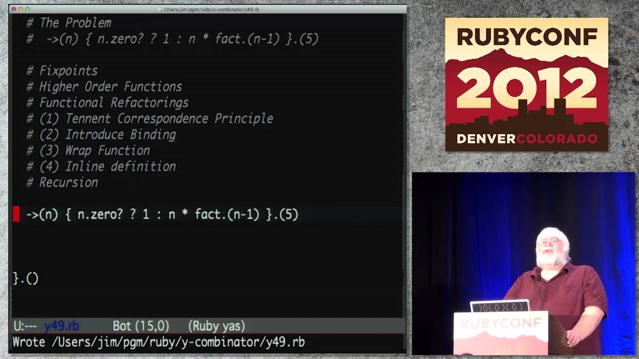
Weirich Derives Y Combinator in Ruby to Solve Anonymous Recursion

Weirich在Ruby中推导Y组合子以解决匿名递归问题 尽管不动点组合子证明了纯lambda演算无需自引用即可实现通用递归，但在支持命名方法的生产代码语言中，它们并没有实际功用。 Jim Weirich展示了如何完全在Ruby中解决lambda演算中的递归悖论——即让匿名函数在不进行自引用的情况下实现递归。在追溯了图灵机与邱奇lambda演算的历史等价性之后，Weirich在展开严谨的现场编码推导前定义了不动点和高阶函数。通过包括腾嫩特对应法则（Tennent's Correspondence Principle）、函数包裹以及内联在内的机械化转换，他将一个脆弱且受深度限制的阶乘改进函数逐步演化为具有自复制特性的应用序不动点组合子（Z组合子）。在此过程中，他说明了惰性求值如何防止过早陷入死循环，并揭示了阶乘本质上就是其自身改进函数的不动点。 艾伦·图灵的图灵机与阿隆佐·邱奇的lambda演算在20世纪30年代各自独立奠定了现代可计算性理论的基础，证明了不具备原生类型的简单模型也能实现完全的图灵完备性。 (2:15) 纯lambda演算缺少具名函数和变量，从而产生了一个悖论：在没有专门的高阶机制的情况下，标准递归调用在句法上是不可能的。 (15:37) 通过从直接自我调用转变为经由生成器函数传递部分实现，仅使用匿名proc即可机械化地合成递归。 (27:34) 在像Ruby这样采用及早求值、应用序的语言中，防止无限递归展开需要将自应用包裹在延迟调用的lambda包装器中，从而形式化推导出Z组合子，而非经典的正规序Y组合子。 (39:30) 尽管不动点组合子在具有命名函数的生产语言中是多余的，但它们的推导过程展示了腾嫩特对应法则和eta展开等函数式重构的强大威力。 (50:33)

In his RubyConf 2012 keynote, Jim Weirich explores Alonzo Church's lambda calculus to demonstrate how pure, anonymous functions can achieve recursion without self-referential names, systematically deriving the applicative fixed-point combinator through semantics-preserving functional refactoring. Foundational Computability and the Recursion Paradox (6:48) In the 1930s, Alan Turing and Alonzo Church independently formulated distinct mathematical frameworks for effective computability: Turing's mechanical tape apparatus and Church's untyped lambda calculus. Although lambda calculus contains no primitive integers, strings, booleans, or assignment operators—relying exclusively on anonymous single-argument functions and beta reduction—mathematicians proved it mathematically equivalent to Turing machines. Church modeled numbers through repeated function composition (Church numerals) and conditionals via branch-selecting functions (Church booleans). An immediate theoretical paradox arises when attempting recursion in this model. Conventional recursive functions, such as factorial, rely on calling an assigned identifier within their own definitions. Because pure lambda calculus permits only anonymous functions without variable assignment, attempting a recursive call without an assigned name raises an undefined reference error, posing the fundamental puzzle of how an anonymous language can remain Turing complete. Mechanical Toolset of Functional Refactoring (21:15) To manipulate anonymous functions systematically, Weirich outlines three behavior-preserving transformations. Tennent's Correspondence Principle establishes that any expression can be wrapped inside a zero-argument anonymous lambda and immediately called without changing its evaluated result. Developers can then introduce a binding by supplying an unused parameter name and passing an argument at the call site, provided the introduced identifier does not shadow any free variables in the inner expression. Function wrapping (eta expansion) encapsulates an existing single-argument function inside an outer lambda that forwards arguments directly to the wrapped target. This operation acts as an identity transformation on execution while serving as a delaying mechanism to prevent premature evaluation. By sequentially inlining named helpers and removing assignment statements, entire functional pipelines can be mechanically collapsed into single, assignment-free lambda expressions. Evolving Partial Improvers into Self-Application (27:34) Attempting to pass a recursive function into a constructor generates an unresolvable circular dependency, as the constructor requires a finished definition to produce that definition. Weirich breaks this cycle by substituting partial definitions. An "improver" function accepts an incomplete function valid over an initial segment of inputs and produces a new function that handles that segment plus one additional depth, falling back to a terminating error stub when limits are exceeded. While chaining improvers manually handles progressively larger values, it remains restricted to finite depths. Weirich eliminates manual chaining by passing the improver directly into itself. Modifying the internal recursive step to pass the generator along—calling the function on itself before applying the numeric decrement—bypasses the need for names and unlocks arbitrary recursion depth, enabling factorials to compute up to the runtime's physical stack limits. Delaying Evaluation to Derive the Fixpoint Combinator (39:30) Decoupling domain-specific arithmetic from the recursion engine reveals an evaluation barrier. In applicative-order languages like Ruby, Python, and Clojure, function arguments evaluate eagerly prior to invocation. Calling self-application directly triggers an immediate stack overflow because the recursion executes unconditionally before evaluating the base case. Weirich remedies this by wrapping the self-application inside a single-argument lambda, deferring evaluation until an argument is supplied. Applying Tennent's Correspondence Principle isolates the pure factorial logic from the recursion plumbing, producing a generic fixed-point combinator. When a fully defined factorial function is passed to the factorial improver, the improver returns that identical function unchanged, demonstrating that factorial is the fixed point of the improver. Because the implementation includes delayed evaluation wrappers for eager execution, it represents the Z Combinator rather than the unwrapped Y Combinator utilized in normal-order, lazy languages like Haskell. Weirich emphasizes that the Y and Z combinators have no direct utility in everyday software development where programming languages natively provide named methods and functions. Instead, the exercise demonstrates the power of functional refactorings to reshape program architectures safely and illustrates how foundational lambda calculus principles underpin modern constructs like Ruby blocks and procs. He references Tom Stuart’s presentation Programming with Nothing as an illustration of constructing complete programs solely out of anonymous lambdas.

Jim Weirich 在 RubyConf 2012 的演讲中论证道：即使在仅允许纯匿名单参数函数的无状态计算模型中，通过函数自应用与语义保持的函数式重构，依然能够推导出通用递归结构；其实质是利用定点组合子（即在及物求值语言中表现为 Z Combinator 的 Y Combinator）求解阶乘等算法的函数不动点。 计算等价性与匿名函数的递归悖论 (2:15) 20 世纪 30 年代，Alan Turing 提出了依赖纸带、读写头和状态转移表的图灵机模型，用以界定“可有效计算”的概念；而 Alonzo Church 则提出了完全抛弃原生数值、字符串与控制流语句的 Lambda 演算（λ-calculus），所有运算均由纯匿名单参数函数抽象与应用构成，两者随后被证明具有完全等价的计算能力（图灵完备）。 然而纯 Lambda 演算带来了一个根本性悖论：所有的计算都是匿名的，不允许将函数绑定到全局变量或函数名。当 Weirich 试图在 Ruby 中直接使用匿名 Proc 计算阶乘时，函数体内因无法引用自身而立即触发 NameError。这一现象引出了演讲的核心理论命题：如果一个计算体系中不存在任何函数命名机制，程序如何实现通用递归以维持其图灵完备性。 代数不动点与递归改进器的概念转化 (12:24) 为解开递归谜题，Weirich 首先以计算器连续按余弦键收敛至 0.739085 为例，引入了不动点（Fixed Point）的数学定义：若 f(x) = x，则 x 即为函数 f 的不动点。普通数学函数作用于数值，而高阶函数则可以作用于函数并产生新的函数，因此函数本身也可以成为高阶函数的不动点。 面对无法自我调用的阶乘函数，Weirich 将思路转变为构造一个“改进器”（factorial_improver）。该改进器接受一个仅能正确处理前 N 个自然数的局部阶乘函数作为参数，并返回一个能处理前 N+1 个自然数的新函数。尽管反复嵌套改进器只能有限拓展计算深度，但它揭示了核心性质：如果将一个完全正确的阶乘函数传给该改进器，改进器将原样返回该阶乘函数，即完全体阶乘函数正是 factorial_improver 的函数不动点。 自应用机制与及物求值下的延迟包装 (31:27) 为了突破手动嵌套改进器的深度限制，Weirich 尝试将改进器作为参数直接传递给其自身（即自应用），从而消除了对基底错误函数的依赖。但在这一过程中，将参数由 partial 替换为自接收的 improver（后更名为 gen）后，直接执行 gen.(gen) 立即触发了系统调用栈溢出（Stack too deep）。 其根本原因在于 Ruby 采用及物求值策略（Applicative-order evaluation），在调用前会提前计算参数值，导致无限展开递归。为了恢复递归终止条件，Weirich 运用了 Eta 展开式函数包装技巧，将立即求值的 gen.(gen) 替换为延迟执行的单参数 Lambda `->(v) { gen.(gen).(v) }`。此举成功将递归调用推迟至实际传入数值参数时触发，使阶乘算法在未命名的匿名自应用下得以正常运行至 2000 级调用限制。 函数式重构与 Z 组合子的形式化隔离 (41:09) 尽管自应用成功实现了阶乘计算，但此时领域数学逻辑与递归底层管道紧密纠缠。Weirich 运用 Tennent 对应原则（Tennent's Correspondence Principle）和引入绑定（Introduce Binding）等纯函数式重构手法，机械化地将纯阶乘逻辑从控制自应用的机制中剥离出来，重构为独立的 improver 函数与通用的组合子 y。 最终提取出的 y 组合子完全不依赖阶乘业务逻辑，其职责是为任意符合改进器形式的高阶函数计算不动点。Weirich 解释指出，在像 Ruby、Python 或 Clojure 这种在传参前先求值参数的及物求值语言中，必须包含延迟包装层，因此在学术分类上该形式严格对应的是 Z Combinator；而在像 Haskell 这类采用正则序（Normal-order）惰性求值的语言中，则直接对应经典 Y Combinator。通过对称化参数重构，该结构最终收敛至计算机科学经典的组合子表达式。 Weirich 强调，在日常工业级软件开发中，由于编程语言均已原生支持具名函数与方法，直接编写 Y 组合子毫无实用价值；但该推导过程的核心价值在于掌握严谨的语义保持式重构技巧，并借此理解底层高阶函数与 Lambda 演算在现代语言抽象机制（如 Ruby 的 Block 与 Proc）中的理论根基。

## Background 本视频由 Confreaks 频道于 2012 年 11 月 11 日在 YouTube 平台发布，记录了 Jim Weirich 在 RubyConf 2012 上的技术基调演讲。视频简介指出，演讲深入探讨了函数式编程领域中最深奥的谜题之一——Y 组合子（Y Combinator），旨在通过推导其运作机制与核心价值，帮助开发者深刻理解函数式编程的本质，即使该模式在日常开发中近乎无用。 ## TL;DR Jim Weirich 从可计算性理论与阿隆佐·邱奇的 Lambda 演算切入，指出了纯匿名函数无法直接命名自引用的“递归死结”。随后，他借助数学上的不动点概念，现场编写 Ruby 代码推导“阶乘改进器”（Factorial Improver），并逐步通过自我传递、延迟求值及坦南特对应原理（Tennent correspondence principle）等函数式重构手法，化解了栈溢出危机。最终，他成功从第一性原理中推导出通用不动点计算器——应用序 Y 组合子（Z 组合子），揭示了极简函数抽象构造通用计算的数学之美。 ## Atmosphere & style 整场演讲兼具极客的硬核幽默与理论推演的严密感。Jim 坦然调侃自己是在展示“最糟糕但最有趣的 Ruby 代码”，并借助台下按计算器的现场实验轻松破冰，营造出亲切而引人入胜的探索氛围。随着现场编码中冗长括号的层层嵌套，以及克服栈溢出崩溃后成功打印出大数阶乘的瞬间，台下爆发出由衷的惊叹与掌声，让听众在烧脑之余充分体验到纯粹逻辑推理带来的顿悟与智识愉悦。 ## Bulletin - [10:00](https://www.youtube.com/watch?v=FITJMJjASUs&t=600s) Lambda 演算与图灵机在有效可计算性上具备等价的图灵完备性，但由于其公理要求所有函数均为匿名且缺乏全局赋值，给递归自引用带来了根本性的理论障碍。 - [45:03](https://www.youtube.com/watch?v=FITJMJjASUs&t=2703s) 数学上的不动点（Fixed-point）满足 f(x) = x；而阶乘函数正是阶乘改进器（Factorial Improver）的高阶不动点，Y 组合子的本质就是通用的不动点计算器。 - [39:30](https://www.youtube.com/watch?v=FITJMJjASUs&t=2370s) 在 Ruby 等及早求值的应用序语言中，直接调用生成器会导致栈溢出无限递归，必须引入显式 Lambda 包装进行延迟求值，所推导出的实际是应用序 Y 组合子（Z 组合子）。 - [50:33](https://www.youtube.com/watch?v=FITJMJjASUs&t=3033s) 尽管 Y 组合子在具备具名函数的现代工程开发中缺乏实用价值，但其机械化重构与纯数学推演展现了纯函数式编程模型解决复杂计算的理论之美。 ## Key takeaways - [03:23](https://www.youtube.com/watch?v=FITJMJjASUs&t=203s) 图灵机仅凭无限纸带、状态转换与简单读写头即定义了有效可计算性，确立了早期计算科学的理论边界。 - [06:48](https://www.youtube.com/watch?v=FITJMJjASUs&t=408s) 邱奇的 Lambda 演算不包含字符串或整数等原生类型，所有计算与布尔逻辑均通过纯函数抽象（丘奇编码）与文本替换式的 β-约归实现。 - [10:00](https://www.youtube.com/watch?v=FITJMJjASUs&t=600s) 图灵机、Lambda 演算与一般递归在表达能力上完全等价，这一理论成果深刻影响了后世各主流现代编程语言中的闭包与匿名函数设计。 - [13:25](https://www.youtube.com/watch?v=FITJMJjASUs&t=805s) 不动点是输入函数后输出原值的元素，反复计算余弦值收敛至常数直观展示了这一性质，为高阶不动点推导奠定了概念基础。 - [15:37](https://www.youtube.com/watch?v=FITJMJjASUs&t=937s) 纯 Lambda 演算禁止变量具名绑定，直接书写递归会导致找不到函数引用的死结，引发了匿名体系如何图灵完备的核心悖论。 - [17:41](https://www.youtube.com/watch?v=FITJMJjASUs&t=1061s) 高阶函数将函数视作一等公民，既能作为参数传入也能动态生成返回，构成了匿名函数组合与变换的基础工具。 - [21:15](https://www.youtube.com/watch?v=FITJMJjASUs&t=1275s) 坦南特对应原理、引入非自由变量绑定与单参函数包装（Eta 扩展）提供了等价重构代码的机械化数学规则。 - [25:18](https://www.youtube.com/watch?v=FITJMJjASUs&t=1518s) 将所有具名函数完全内联为嵌套 Lambda 证明了无需赋值语句即可通过传参绑定完成复杂数值计算。 - [27:40](https://www.youtube.com/watch?v=FITJMJjASUs&t=1660s) 阶乘改进器（Factorial Improver）将完备阶乘拆解为扩充局部定义的渐进步骤，绕开了直接生成全量递归函数的死循环。 - [32:36](https://www.youtube.com/watch?v=FITJMJjASUs&t=1956s) 打破无名递归禁区的关键在于让生成器函数接受自身作为参数（自我吞噬），从而在内部构造出递归调用的能力。 - [39:30](https://www.youtube.com/watch?v=FITJMJjASUs&t=2370s) 应用序语言急切求值的特性会导致自调用参数提前计算，必须使用单参 Lambda 包裹实现延迟求值以防止调用栈溢出。 - [41:42](https://www.youtube.com/watch?v=FITJMJjASUs&t=2502s) 通过 Tennent 重构将通用的递归生成脚手架与阶乘的具体业务逻辑彻底解耦，提炼出通用的递归组合子抽象。 - [45:03](https://www.youtube.com/watch?v=FITJMJjASUs&t=2703s) 阶乘函数输入阶乘改进器后仍原样输出阶乘函数，证明阶乘是不动点，而 Y 组合子就是接收改进器并求解其不动点的高阶算子。 - [47:05](https://www.youtube.com/watch?v=FITJMJjASUs&t=2825s) 学术界经典的 Y 组合子适用于正常序惰性求值语言，而在 Ruby/Python 中推导出的需显式防无限展开的版本实际上被称为 Z 组合子。 - [50:33](https://www.youtube.com/watch?v=FITJMJjASUs&t=3033s) Y 组合子的推导演示了从第一性原理仅凭极简规则演化出通用计算能力的纯粹数学之美。 ## Detailed walkthrough ### [00:00](https://www.youtube.com/watch?v=FITJMJjASUs&t=0s) 开场：不合常规的技术基调演讲 Jim Weirich 热情向 RubyConf 的观众打招呼并引出当天的核心主题——Y 组合子（Y Combinator）。当他询问现场有多少人对 Y 组合子非常熟悉时，台下举手的人屈指可数，这让 Jim 幽默地感叹道：“That means I can say anything I want to about it.”（这说明我可以畅所欲言了）。 Jim 接着分享了自己长期作为演讲者的经验。他调侃基调演讲（Keynote）通常遵循的三大不成文规矩：第一，基调演讲通常不宜过于技术化，而是要侧重激励与鼓舞人心，但他宣布这场演讲将是“高度偏向技术”的；第二，如果是硬核技术演讲，往往应贴近程序员日常工作，提供带回办公室即可使用的实用技巧，但他直言：“I am glad to say that this talk is extremely pointless.”（我很高兴地宣布，这场演讲极其毫无意义），听众几乎不可能把它直接运用到工作中；第三，既然缺乏实用性又偏技术，至少代码范例应该展示良好编码规范，但他坦率承认：“I am also happy to say this will be the worst Ruby code you've probably ever seen.”（我也很高兴地说，这大概会是你们见过的最糟糕的 Ruby 代码）。整场演讲唯一的价值，就是带来纯粹的思维乐趣。 - 核心演讲主题：深入解析函数式编程核心概念 Y 组合子 - 演讲违背的常规 Keynote 惯例： - 内容极度技术化而非宽泛激励 - 缺乏业务实用性与直接落地价值 - 代码示例不符合日常整洁规范，专为理论推演设计 ### [02:15](https://www.youtube.com/watch?v=FITJMJjASUs&t=135s) 现场实验：反复计算余弦的不动点伏笔 在展开理论之前，Jim 向台下征集了一位带有计算器、且支持弧度制计算余弦值（cosine）的观众。一名后排观众带着计算器走上前台配合互动。 Jim 给出的指令十分简单：先输入数字 0，确保计算器处于弧度制模式（radians mode），按下 $\cos$ 键得到结果后，不要停下，反复继续按 $\cos$ 键。Jim 叮嘱对方：“Keep doing that until I get back to you.”（一直按下去，直到我回头找你），这一神秘的互动在引发现场欢笑的同时，为后文关于数学不动点（Fixed-point）与递归组合子的讨论埋下了伏笔。 ### [03:23](https://www.youtube.com/watch?v=FITJMJjASUs&t=203s) 图灵机与有效可计算性 演讲的核心命题是“有效可计算性”（effectively computable）。Jim 带领观众回到计算机科学萌芽的 1930 年代，首先介绍了艾伦·图灵（Alan Turing）以及图灵机（Turing machine）模型。图灵机概念精简至极：一条带有格子（cell）的无限长纸带、一个可在格子上读取/擦除/写入字符的读写头，以及控制纸带单格左右移动的极其简易的状态转移规则。 Jim 展示了一段实体机械图灵机的视频演示。该装置配备带光源的摄像头来识别当前符号，通过擦头与写头完成 0 和 1 的修改，正以二进制形式依次递增数字计数（从 11、12、13 到 14、15，最终完成进位并停机）。Jim 借此赞叹图灵敏锐深邃的洞察力：在第一台可编程计算机于德国问世（约 1936 年）之前，图灵在 1936 至 1937 年间完全仅凭纸笔和纯脑力思考，就奠定了整个理论体系。Jim 指出：“Turing said that anything that is effectively computable can be computed by this really dirt-simple machine, this Turing machine.”（图灵提出，任何有效可计算的事物，都可以由这台极度简陋的机器——图灵机——计算出来）。 ```mermaid flowchart LR accTitle: 图灵机基础运作循环 accDescr: 展示图灵机读写头对纸带格子的读取、擦写与位移循环 subgraph Tape["无限纸带 (Infinite Tape)"] Cell["当前单元格 (Cell)"] end subgraph Head["读写与控制系统"] Read["摄像头/读头 (Read)"] Decide["状态转换控制程序"] Write["擦除并写入 (Erase & Write 0/1)"] Move["左右移动一格 (Shift Tape)"] end Cell --> Read Read --> Decide Decide --> Write Write --> Move Move --> Cell ``` ### [06:48](https://www.youtube.com/watch?v=FITJMJjASUs&t=408s) 邱奇的 Lambda 演算与丘奇编码 大约在图灵提出图灵机的同时，阿隆佐·邱奇（Alonzo Church）提出了 Lambda 演算（$\lambda$-calculus）。Jim 拆解了 Lambda 演算的基本构造：以字符 $\lambda$ 引入一个函数，后跟变量名（如 $x$），接着用点号（$.$）将变量名与函数体分隔。最简单的函数就是恒等函数 $\lambda x. x$，传入任何值便原样返回该值。 令人震惊的是，Lambda 演算的世界里不存在字符串、整数或浮点数等任何常规数据类型，有的仅仅是“函数以及对函数的调用”。为了表达计算世界中的各种概念，必须依靠纯函数进行编码，即丘奇数（Church numerals）： - 数字 $1$：写作接收函数 $f$ 和参数 $x$ 的函数（$\lambda f. \lambda x. f(x)$），将 $f$ 应用于 $x$ 一次； - 数字 $2$：将函数 $f$ 连续调用两次（$\lambda f. \lambda x. f(f(x))$）； - 数字 $0$：对参数调用函数 $f$ 零次（$\lambda f. \lambda x. x$）； - 布尔值 $\text{True}$ 与 $\text{False}$：$\text{True}$ 是接受两个参数并返回第一个参数的函数（$\lambda x. \lambda y. x$），充当类似 if-then-else 中的 then 分支；而 $\text{False}$ 则返回第二个参数（$\lambda x. \lambda y. y$），充当 else 分支。 - Lambda 演算的三大支柱规则： - 数据类型单一性：函数是唯一的合法数据类型，无任何内置基本类型 - Lambda 绑定（Lambda binding）：值与变量名关联的唯一方式就是函数调用传参 - 核心化简机制：通过 $\beta$-约归（Beta reduction）展开函数体并进行代换，辅助机制为 $\alpha$-变换（Alpha conversion） ### [10:00](https://www.youtube.com/watch?v=FITJMJjASUs&t=600s) $\beta$-约归、宏展开与图灵完备等价性 Jim 现场推导了一个 $\beta$-约归的直观示例：将布尔值 $\text{True}$ 依次作用于参数 $1$ 与参数 $0$。在第一步 $\beta$-约归中，找到形参 $x$ 并将实参 $1$ 替换进函数体内；接着在第二步中对形参 $y$ 与实参 $0$ 展开，由于函数体中不再依赖 $y$，最终直接返回 $1$。 Jim 总结道，Lambda 演算的底层逻辑归根到底就是文本替换式的宏展开（macro expansion）。然而，邱奇甚至比图灵早两三年（大约在 1933 到 1935 年间）就发表了论文并提出论断：“Church said, 'Anything that can be effectively computable can be computed via lambda calculus.'” 随后数学界就图灵机与 Lambda 演算所能计算的问题集是否等价展开了长久辩论，最终证实图灵机、Lambda 演算以及同时期发展的一般递归（general recursion）三者在能力上完全一致，即全都是“图灵完备”（Turing complete）的。 ### [12:24](https://www.youtube.com/watch?v=FITJMJjASUs&t=744s) Lambda 演算的现实回响与图灵完备性 可计算函数无论是在丘奇的 Lambda 演算、哥德尔的一般递归理论，还是图灵机中，计算能力都是完全等价的。Lambda 演算的思想深远地渗透到了现代编程语言的血脉之中：Lisp 充斥着 lambda；Clojure 的匿名函数 `fn` 本质上就是 lambda；Ruby 甚至因为太喜欢 lambda 而提供了多种定义语法；CoffeeScript 具备极其简洁的 lambda 表达形式；JavaScript 自身也内置了对 lambda 的支持。这些匿名函数无非就是闭包或 lambda。在昨天的技术分享中，如果听众参加了 Pat 探讨代码块的演讲，就已经理解了闭包的机制。 在赞叹现代语言对函数式特性的采纳之余，必须正视一个看似反直觉的事实：极其简陋的 Lambda 演算竟然是图灵完备的。这背后隐藏着一个棘手的逻辑冲突，但在揭晓冲突之前，需要先收回上一节埋下的伏笔。 - 现代语言中的 Lambda 形式：Lisp (`lambda`)、Clojure (`fn`)、Ruby (Stabby proc `->`)、CoffeeScript (`->` / `=>`)、JavaScript (`function` / 箭头函数)。 - 匿名函数的核心本质即为闭包（Closure）与 Lambda 演算中的抽象。 ### [13:25](https://www.youtube.com/watch?v=FITJMJjASUs&t=805s) 寻找余弦的不动点：从按计算器到数学定义 演讲现场的伏笔揭晓，此前拿到科学计算器的观众公布了反复按动余弦（cosine）键的最终结果：0.739085。在掌声中，Jim Weirich 解释了这一现象的数学原理：从 0 开始取弧度制余弦得到 1，再取 1 的余弦得到约 0.54；若坚持重复该操作大约 89 到 90 次（具体取决于浮点运算精度），数值便会逐步收敛至 0.7390851…… 这个数值被称为余弦函数的“不动点”（Fixpoint）。 ```mermaid flowchart LR accTitle: 不动点概念示意图 accDescr: 展示将数值输入函数后输出原数值的不动点收敛特征 subgraph S1["不动点变换过程"] X["输入 x"] --> F["函数 f(x)"] F --> FX["输出 f(x) = x"] end ``` 所谓不动点，定义极其纯粹：“A fixpoint is nothing more than a value you give to a function and if that functions returns the same value then that is a fixpoint.”。其形式化定义为：若 $f(x) = x$，则 $x$ 是函数 $f$ 的不动点。不同函数的不动点性质各异： - 余弦函数（$\cos$）：可以通过反复迭代收敛至特定的常数（Dottie 数约 0.739085）。 - 正弦函数（$\sin$）：具有更简单的不动点 0，因为 $\sin(0) = 0$。 - 平方根函数（$\sqrt{x}$）：具有两个不动点，因为 $\sqrt{0} = 0$ 且 $\sqrt{1} = 1$。 - 恒等函数（$I(x) = x$）：任何输入值都是其不动点，拥有无穷多个不动点。 - 亦有部分函数完全不存在任何不动点。 这个概念是理解后续理论的核心基石，需要牢牢记在脑海中。 ### [15:37](https://www.youtube.com/watch?v=FITJMJjASUs&t=937s) Live Coding 开启：匿名函数中的递归死结 演示切换至现场代码编写环节。环境使用 Ruby 1.9 引入的 Stabby Proc 语法 `->(arg) {... }`，并通过点号括号语法 `.()` 进行调用，缓冲区设置成每次求值直接输出最后一行表达式的结果。 Jim Weirich 试图在代码中写出一个简单的阶乘函数：若参数为 0 则返回 1，否则返回 `n` 乘以 `n - 1` 的阶乘。如果将其实例化为一个变量 `fact` 并传入 5，系统能够正确计算出 120。然而，Lambda 演算的底层公理带来了一个致命危机：在纯粹的 Lambda 演算体系中，根本不允许给表达式进行具名赋值，一切函数都必须以匿名 lambda 的形式直接定义并就地调用。当试图把函数命名拿掉、单纯以内联匿名表达式执行时，代码立即崩溃并报错未定义方法或变量 `fact`。 这是因为在函数体内部引用了外部尚未绑定完成的名字 `fact`。全场最关键的悖论随之浮现：“Well in lambda calculus all functions are anonymous, so how in the world can I define that factorial without referring to itself? That's a problem.”。如果一切函数都是匿名的，无法进行自引用命名，递归要如何发生？如果连自递归都做不到，Lambda 演算又怎么可能是图灵完备的？为了解开这个死结，必须先行掌握高阶函数与函数式重构这几个理论武器。 - 阶乘测试用例：`fact.(5)` 应返回 `120`。 - 核心困境：没有全局环境，没有变量赋值，匿名函数无法通过名字直接调用自身实现递归。 ### [17:41](https://www.youtube.com/watch?v=FITJMJjASUs&t=1061s) 武器库第一件：高阶函数与组合 理解匿名递归的前提是彻底掌握高阶函数（Higher-Order Functions）。在 Ruby 中，像 `each` 这样的方法本身就是一种高阶函数。常规函数非常直观，例如接受数值并加 1 的 `add_one`，或是将数值乘以 3 的 `mul_three`，它们接收基本数据并返回计算后的数据。 高阶函数则打破了这种界限，它将“函数视为一等公民（First-class values）”。第一类高阶函数能够“生成并返回新函数”，例如 `make_adder`：它接受一个参数 `x`，返回一个闭包函数 `->(n) { x + n }`。有了它，甚至可以直接写出 `add_one = make_adder.(1)`。第二类高阶函数不仅能返回函数，还能“接收函数作为输入参数”，例如函数组合器 `compose`：它接受函数 `f` 与 `g`，返回一个将二者串联调用的新函数 `->(n) { f.(g.(n)) }`。通过 `mul_three_add_one = compose.(mul_three, add_one)`，传入 10 可以依次执行加 1 得 11、乘 3 得 33。 函数不再只是执行逻辑的容器，而是可以像字符串、整数一样被自由传递、包裹、组装的操作对象。 ### [21:15](https://www.youtube.com/watch?v=FITJMJjASUs&t=1275s) 函数式重构法则：坦南特原理、引入绑定与函数包装 就像面向对象编程拥有“提炼方法”或“折叠继承体系”等重构手段一样，函数式编程也有一套纯粹、机械化且不改变程序外在行为的代码重构手法。 第一项重构是**坦南特对应原理（Tennent correspondence principle）**。其核心内涵极其简练：如果存在一个表达式 `x`，用一个无参匿名 lambda 将其包裹并立即执行 `-> { x }.()`，其计算结果依然是 `x`，对原有逻辑完全无害。Jim Weirich 在编辑器中现场演示了这一过程，先是手动将 `mul_three` 内部的逻辑用 lambda 包装并立即调用，随后甚至调用 Emacs 编辑器宏全自动执行这一包装，输出结果始终稳固在 33。这种变换完全是机械化的语法等价代换。 第二项重构是**引入绑定（Introduce a binding）**。在已经建立的无参 lambda 外部包裹上添加一个形式参数（例如 `z`），并在调用处传入任意一个虚拟值 `->(z) { expr }.(val)`。只要 `z` 在函数体内从未被读取，传入什么值都无关紧要。但这里存在一条严格的变量作用域铁律：新引入的形式参数绝对不能遮盖（shadow）原表达式中的“自由变量（Free variables）”。在组合逻辑中，如果表达式内部引用了外部作用域定义的 `f` 和 `g`，那么新变量名就绝不能取名为 `f` 或 `g`，否则外部函数引用会被破坏导致程序崩溃；相比之下，取名为未被占用的名字（比如无厘头的 `xyzzy`）则绝对安全。 第三项重构是**函数包装（Wrap function，即 Eta 扩展）**。如果手上有一个接受单参数的函数表达式，可以将其外层嵌套一个新的单参 lambda `->(v) { fn.(v) }`，并将参数 `v` 透传给内层函数调用。这在不改变原有函数签名和执行效果的前提下，为后续的逻辑解耦与参数延迟求值提供了操作空间。 - 坦南特对应原理：`expr` 等价于 `-> { expr }.()`。 - 引入绑定法则：`-> { expr }.()` 等价于 `->(var) { expr }.(arbitrary_val)`，前提是 `var` 不在 `expr` 的自由变量集合中。 - 函数包装法则：单参函数 `f` 等价于 `->(v) { f.(v) }`。 ### [25:18](https://www.youtube.com/watch?v=FITJMJjASUs&t=1518s) 最后的预备重构手段：延迟计算与极端内联 在正式解决递归问题前，Jim Weirich 演示了最后两种重构技巧。首先是“函数包裹”（Function Wrapping）。将一段求值逻辑包裹在一个无参 lambda 内部并不会改变最终的计算结果（依然能正确算出 33），但它起到了延后执行的作用。Jim Weirich 解释这种模式的价值所在：“It's kind of like a delaying tactic. If you don't want to evaluate something right away, this is something you can do to do that.” 只有在显式调用这个外层 lambda 时，内部的代码才会真正被求值，因此函数包裹是一种完全合法的重构操作。 接着，Jim 演示了让观众忍俊不禁的“内联定义”（Inline Definition）。他指出，代码中的任何命名定义（如 `make_adder`）都可以直接被机械地替换为其底层的 lambda 实现。他逐步对 `compose`、`add_one`、`mul_three` 等命名函数展开彻底的内联替换。随着层层括号不断嵌套堆叠，屏幕上的代码变得无比冗长晦涩。面对全场的笑声，Jim 幽默地调侃道：“I did promise you the worst ruby code you'd ever see, right?” 然而当他按下回车执行这串杂乱无章的代码时，屏幕上依然稳定地返回了 33，引来台下一片掌声。 ```mermaid flowchart LR accTitle: Pure Lambda Expression Execution accDescr: Transformation from named function calls into a single pure nested lambda expression producing the value 33. subgraph S1["代码重构过程"] A["命名函数体系<br/>(make_adder, compose 等)"] -->|"机械式内联替换"| B["单一纯 Lambda 表达式<br/>(无变量赋值)"] end subgraph S2["求值输出"] B -->|"参数逐步绑定求值"| C["返回正确结果 33"] end ``` 这段极端内联的代码揭示了 Lambda 演算（Lambda Calculus）的核心本质： - **消除所有赋值**：整个表达式中没有出现任何变量赋值语句（`=`）。 - **仅靠参数绑定**：变量与名称的唯一绑定机制就是调用这些匿名 lambda 函数并传参。 - **理论意义**：尽管这种代码在日常开发中极难阅读且不推荐编写，但它证明了 Lambda 演算的终极目标——通过一个巨大的、纯粹的 Lambda 表达式来完成复杂的数学计算。 --- ### [27:40](https://www.youtube.com/watch?v=FITJMJjASUs&t=1660s) 阶乘递归的死结与“阶乘改进器”（Fact Improver）概念的提出 完成预备知识铺垫后，Jim 删除了之前的练习代码，重新回到讲座的核心议题——实现递归阶乘函数。在 Lambda 演算的规则下，所有函数都是匿名的。如果在 `factorial` 的定义内部根本无法通过名字引用 `factorial` 本身，递归究竟该如何实现？Jim 首先尝试了一种间接思路：定义一个 `make_factorial` 函数，把 `factorial` 当作参数传进去以实现名称绑定。但随之而来的致命死循环是：要调用 `make_factorial` 创造阶乘函数，就必须先传入一个现成的 `factorial` 定义。正如 Jim 所说：“That's not going to work because to make a factorial I need the definition of factorial.” 为了打破这一循环论证，Jim 退后一步，降低了要求，提出了极具启发性的“阶乘改进器”（Factorial Improver）模型。他不奢求立刻一步到位生成完整的阶乘函数，而是让这个高阶函数接收一个“部分定义”（Partial Definition）作为参数： - **部分定义的含义**：一个仅在输入子集上能正确计算阶乘的函数（例如只能处理 0 到 10 的整数）。 - **改进器的产出**：将该部分定义输入 `fact_improver` 后，它会返回一个功能扩充一步的新函数（支持计算 0 到 11 的阶乘）。 为了验证这个模型，Jim 先编写了一个只要被调用就会报错的辅助函数 `error`。随后他演示了递推的过程： 1. 将 `error` 传入 `factorial_improver`，生成了函数 `f0`。因为计算 0 的阶乘走的是基本情况（Base Case，返回 1），根本不会触发递归分支，所以 `f0(0)` 成功返回 1；但 `f0(1)` 会触发 `error`。 2. 将 `f0` 传入改进器生成 `f1`，此时 `f1(1)` 顺利计算出 1，但在计算 2 时失败。 3. 依此类推，将 `f1` 传入得到 `f2`，便可成功计算 2 的阶乘。 为了摆脱对外部命名的依赖，Jim 将这一连串调用内联展开。他把调用片段复制粘贴了五次并平衡括号，得到了一个匿名函数 `fx`。这个经过五层包裹的 `fx` 能够成功算出 5、10 乃至 14 的阶乘，但在计算 15 时会因底层的 `error` 崩溃。Jim 调侃道：“All I have to do is decide the biggest number I will ever want the factorial of and call fact improver on it that many times.” 但这种硬编码展开显然不是真正的通用阶乘函数。 --- ### [32:36](https://www.youtube.com/watch?v=FITJMJjASUs&t=1956s) 自我吞噬的奇迹：将 Improver 传递给自身 为了走向真正的纯 Lambda 演算，Jim 运用“嵌入到 Lambda”的技巧，将改进器作为参数 `improver` 传给一个外层 Lambda。此前，最底层的兜底参数一直是一个与阶乘毫无关系的 `error` 函数。Jim 突发奇想：如果不用 `error`，而是直接将 `improver` 自身传给 `improver` 会发生什么？ 试验结果显示： - 调用 `fx(0)` 成功返回 1。 - 但调用 `fx(1)` 时，Ruby 抛出了异常：`TypeError: Proc can't be coerced into Fixnum`。 - 崩溃的原因显而易见：在执行到乘法运算 `n * partial(...)` 时，由于传入的不再是普通的阶乘函数，而是 `improver` 自身，而 `improver` 期望接收的是一个函数而非数字 `n - 1`。 既然 `improver` 期望接收一个函数，而当前作用域里恰好就有一个可用的函数——`improver` 自身，Jim 便顺理成章地将代码中的调用改写为 `improver.call(improver)`。全场屏息以待这个看似不可思议的递归拼接。Jim 笑着说：“Gosh, I wonder if this could possibly work.” 测试的结果令人震撼： - `fx(1)` 成功返回 1； - `fx(2)` 成功返回 2； - `fx(5)` 成功返回 120； - 紧接着 Jim 一路测试了 50、500，甚至直接测试了 2000 的阶乘（在调用栈溢出前支持的最大极限）。 最后，Jim 将整个逻辑内联为一段完全自包含的 Lambda 表达式，并在末尾直接传入参数 5，屏幕上干脆利落地打印出了 120。台下爆发出了热烈的掌声。通过让函数将自身作为参数传递的机制，无名函数彻底打破了无法递归的禁区。 --- ### [36:12](https://www.youtube.com/watch?v=FITJMJjASUs&t=2172s) 重构起点：命名辨析与坦南特对应原则的应用 尽管上述方案已经在纯 Lambda 表达式下完美运行，但 Jim 对这段代码的现状并不满意，指出了两个深层次的问题： 1. **参数语义失真**：内部绑定的形参原本叫 `improver`，但实际上它接收的已经不再是一个部分阶乘定义，而是一个接收自身的函数。Jim 坦言自己找不到现成术语来描述它：“I'm going to go with the name gen, because it's a generator that somehow when you feed it itself, when it swallows itself, it generates a recursive function.” 因此他决定将其重命名为 `gen`（生成器）。 2. **缺乏直观性与通用性**：这段代码包含了大量为了实现递归而妥协的低层机械结构（如显式调用 `gen.call(gen)`）。Jim 强调：“The second thing is that if I were to sit down and write a recursive function it would never in my entire life occur to me to write it in this manner.” 相比之下，最开始编写的“阶乘改进器”思路（接受一个类似阶乘的函数并扩展一步）显得非常自然。他希望通过重构，把通用的递归驱动机制与纯粹的阶乘业务逻辑剥离开来。 为了将代码形态重新还原为优雅的“改进器”模式，Jim 开始对内层 Lambda 进行重构。他再次运用了坦南特对应原则（Tennent's Correspondence Principle）： - 在内层表达式外包裹一层新的 Lambda 并立即调用它，验证程序行为保持不变； - 引入一个新的形参绑定 `code`，初始时给它传入之前用过的 `error` 占位函数。由于函数体内尚未真正使用 `code`，阶乘计算依然正常返回 120； - 随后他将传入的实参从 `error` 替换为作用域内的生成器 `gen`，程序依然稳健运行，为接下来将生成逻辑抽离成 Y 组合子做好了铺垫。 ### [39:30](https://www.youtube.com/watch?v=FITJMJjASUs&t=2370s) 延迟求值：用 Lambda 包装解决栈溢出 当 Jim Weirich 尝试将整个 `gen(gen)` 当作普通函数直接调用时，程序立刻崩溃并抛出错误：“Oops. Stack too deep.”（调用栈过深）。Jim 解释了事故的原因：在之前的代码里，`gen` 只有在 $n$ 不为 0 时才会递归调用自身，存在递归终止条件（bottomed out）；但如果把 `gen(gen)` 作为参数无条件求值并传入，即使当 $n=0$ 时也会无休止地提前执行 `gen(gen)`，从而陷入无限递归。面对这个问题，Jim 提出了函数式编程的核心思想：“If there were only some way of delaying evaluation. Let's wrap it in a function.”（如果能有某种延迟求值的方法就好了。让我们把它包装进一个函数里。） Jim 引入了一个接收参数 `v` 的匿名函数（`->(v) {... }`），用这个包装函数替换掉了原本直接调用的 `gen(gen)`。由于 Ruby 只有在实际调用该 Lambda 时才会执行内部逻辑，参数传递时仅仅是传递了这个函数引用，避免了无休止的递归展开，测试运行后再次成功算出了结果。紧接着，Jim 发现内部的一段代码与传递给 `code` 的逻辑完全一致，于是顺理成章地用 `code` 进行了替换。此时，被包装出来的核心代码段忽然呈现出熟悉的结构，Jim 随之将 `code` 重命名为 `partial`，兴奋地发现最初构造的阶乘改进器（improver）竟然自然而然地重新浮现了。 ```mermaid flowchart TD accTitle: 延迟求值与递归保护流程 accDescr: 展示将直接调用 gen(gen) 转化为 lambda 包装以延迟求值的逻辑演变 subgraph Problem["无限递归崩溃"] A["直接求值 gen(gen)"] -->|"提前求值，无视 n==0"| B["Stack too deep (栈溢出)"] end subgraph Solution["延迟求值 (Lazy Evaluation)"] C["->(v) { gen(gen).call(v) }"] -->|"仅传递函数定义，不立即运行"| D["仅在需要时被触发"] D --> E["终止条件生效，计算 120"] end ``` ### [41:42](https://www.youtube.com/watch?v=FITJMJjASUs&t=2502s) 提炼函数：解耦通用递归逻辑与业务逻辑 虽然阶乘改进器重新显现，但它依然深埋在负责自引用的递归脚手架代码中。为了将其彻底解耦，Jim 再次运用了 Tennent 重构原则（Tennent Refactoring），将不包含外层调用的主体逻辑整体包裹进一个新的 Lambda 中，并通过格式化和缩进理清层次。他再次熟练地引入了一个临时绑定 `code = error`，确认代码能够正常运行输出 120。随后，他将内嵌的改进器逻辑完整复制并作为参数赋给 `code`，再将内部硬编码的改进器实现替换为对 `code` 的调用。 在这个重构过程中，Jim 讲了一个幽默的小插曲：“I was practicing this this morning and I was typing improver so often all of a sudden I started reading it as imp rover.”（我今天早上练习这段代码时，improver 打得太频繁了，以至于我脑子里突然把它读成了‘小恶魔漫游者’[imp rover]。）在笑声中，他把局部变量 `code` 正式重命名为 `improver`。此时代码形成了清晰的分工：一部分纯粹处理问题的递归自引用性质，而另一部分则是唯一知晓阶乘业务规则的 `improver`。Jim 随即把各个部分分别抽离并赋予具名变量：负责阶乘核心逻辑的命名为 `fact_improver`，处理递归组合机制的抽象命名为 `y`，两者的结合则赋给最终的真实阶乘函数 `fact`。 - 整个重构过程中，阶乘逻辑与递归实现机制彻底分离，外部业务完全感知不到底层繁琐的 Lambda 嵌套。 - 提取出的三大组件层级清晰：`fact_improver` 掌管数学规则，`y` 掌管递归抽象，`fact` 为两者的结合体。 ### [45:03](https://www.youtube.com/watch?v=FITJMJjASUs&t=2703s) 不动点理论与 Y 组合子本质 在整理好代码后，Jim 从最底层的阶乘函数切入，逐步揭示函数式编程中极具美感的核心数学概念——不动点（Fixed Point）。他首先演示，将最终的 `fact` 传给验证测试，能够准确计算出 5 的阶乘为 120。紧接着他提出了一个问题：如果将真实的阶乘函数 `factorial` 再次丢进 `fact_improver` 会发生什么？理论上，改进器接收一个偏函数并将其能力向前推进一步；但如果输入本身就已经是完美的阶乘函数，它所能做的就只有原封不动地返回该函数本身。Jim 现场运行了测试，结果依然稳定输出 120，这证明了对于 `fact_improver` 来说，它的输入就是它的输出。 Jim 由此给出了核心结论：“Factorial is the fixpoint of fact improver.”（阶乘就是阶乘改进器的不动点。）他进一步阐释，不仅普通数学方程具有不动点，高阶函数同样拥有不动点，只是高阶函数的不动点本身也是一个函数。进而，函数 `y` 的本质也就真相大白了：函数 `y` 实际上是一个通用的不动点计算器，它专门用来计算任何以改进器风格编写的递归函数的不动点，无论是阶乘还是斐波那契数列，均能通用。这正是大名鼎鼎的 **Y 组合子（Y Combinator）**，由于专门求解不动点，它也被称为不动点组合子（Fixpoint Combinator）。 ```mermaid flowchart LR accTitle: 不动点与 Y 组合子的映射关系 accDescr: 展示函数 y 如何接收 improver 并输出其对应的不动点函数 subgraph FixpointConcept["不动点概念"] F["factorial"] -->|"输入给 fact_improver"| F end subgraph YCombinatorRole["Y 组合子的职责"] Y["Y 组合子 (y)"] -->|"作用于 improver"| Fix["计算出不动点 (如 factorial)"] end ``` ### [47:05](https://www.youtube.com/watch?v=FITJMJjASUs&t=2825s) 应用序 Y 组合子（Z 组合子）与数学对称性 Jim 解释了为何在维基百科上查到的 Y 组合子与现场推导的版本略有出入。首先是命名习惯：“First of all, mathematicians don't like intention-revealing names.”（首先，数学家不喜欢能表达意图的变量名。）数学家习惯将具有明确语义的 `improver` 简写为 `f`，将生成函数 `gen` 简写为 `x`。其次，更为关键的差异在于求值策略：标准的 Y 组合子适用于正常序（Normal Order）语言（例如 Haskell 这种惰性求值语言）；而像 Ruby、Python、Lisp 和 Clojure 这些语言均属于应用序（Applicative Order）语言，它们在将参数传入函数之前就会立即求值。为了防止像前面演示的那样触发无限递归，必须引入一个类似 `->(v) {... }` 的包装函数。因此，严格来说在 Ruby 中推导出的版本属于**应用序 Y 组合子**，在学术上也常被称为 **Z 组合子（Z Combinator）**。 随后，Jim 展示了如何通过两次等价重构将当前的实现转化为学术界最经典的形式。由于 `f` 代表阶乘改进器，对不动点外层再包一层 `f` 属于空操作（no-op）；再加上一层函数包装并调整缩进后，代码的主体结构与传入参数的形式呈现出了惊人对称的双重结构。至此，Jim 成功完成了从最基础的第一性原理（first principles）到标准学术形态 Y 组合子的完整推导，现场响起了热烈的掌声。 | 组合子名称 | 求值策略 (Evaluation Strategy) | 典型应用语言 | 是否需要显式 Lambda 包装 (`->(v)`) | |:--- |:--- |:--- |:--- | | **标准 Y 组合子** | 正常序（Normal Order / 惰性求值） | Haskell | 否（语言原生延迟求值） | | **Z 组合子 (应用序 Y)** | 应用序（Applicative Order / 急切求值） | Ruby, Python, Clojure, Lisp | 是（防止栈溢出死循环） | ### [50:33](https://www.youtube.com/watch?v=FITJMJjASUs&t=3033s) 总结与延伸：Lambda 演算的纯粹魅力 “Wow, my brain is dead after that one.”（哇，讲完这个我的大脑已经死机了。）Jim 坦率地舒了一口气。他回顾了自己探究 Y 组合子的初衷，单纯是因为听说过太多次而极其渴望彻底弄懂它。对于开发者常问的“如何把 Y 组合子用在自己的实际代码中”，Jim 给出了非常诚恳的忠告：如果你身处一个支持具名函数的现代编程语言中，你根本不需要 Y 组合子；除非你想把所有代码通通写成纯粹的匿名函数，但现实中绝不推荐这么做。 然而，推导 Y 组合子的价值不在于工程实用性，而在于其思想深度与思维训练。Jim 总结道：“I think the y combinator is one of those examples of great beauty in mathematics.”（我认为 Y 组合子是数学中绝美事物的典范之一。）它生动展示了如何仅凭极度抽象、类似简单宏替换的 Lambda 演算规则，逐步演化出强大的计算与递归能力，而这种思想深植于 Ruby 乃至现代编程的底层。在演讲的尾声，Jim 向对该领域意犹未尽的观众极力推荐了 Tom Stuart 的经典演讲《Programming with Nothing》。在该演讲中，Tom 完全不用整数、字符串或任何控制流逻辑，仅凭 Lambda（stabby procs）就纯手工实现了 FizzBuzz 程序，是 Ruby 展现 Lambda 演算纯粹魅力的极致典范。Jim 鼓励大家检索观看该演讲，并在观众热烈的掌声中结束了本次分享。 ## Notable quotes > [50:33](https://www.youtube.com/watch?v=FITJMJjASUs&t=3033s) I think the y combinator is one of those examples of great beauty in mathematics. — Jim Weirich > [13:25](https://www.youtube.com/watch?v=FITJMJjASUs&t=805s) A fixpoint is nothing more than a value you give to a function and if that functions returns the same value then that is a fixpoint. — Jim Weirich > [39:30](https://www.youtube.com/watch?v=FITJMJjASUs&t=2370s) If there were only some way of delaying evaluation. Let's wrap it in a function. — Jim Weirich ## Mentioned Jim Weirich, Alan Turing, Alonzo Church, Tom Stuart, Paul Graham, Pat, Y-Combinator, RubyConf, Turing machine, Lambda calculus, Programming with Nothing, Emacs, Ruby, Clojure, Lisp, Haskell, JavaScript, CoffeeScript, Python ## Video description One of the deepest mysteries in the functional programming world is the Y-Combinator. Many have heard of it, but few have mastered its mysteries. Although fairly useless in real world software, understanding how the Y-Combinator works and why it is important gives the student an important insight into the nature of functional programming. Join with us on this journey of understanding. Be prepared to curry your functions and bind your lambdas as we delve into the whys and wherefores of this paragon of functional programming. Although you will probably never have a need for the combinator, the effort put forth to understand it will improve your functional programming chops. This talk is not for the faint of heart, but the successful student will be richly rewarded. Also, you will understand why "Y-Combinator" is the perfect name for Paul Graham's start-up funding company. At the end of his talk Jim references Tom Stuart's talk "Programming with Nothing" which can be found here: https://www.youtube.com/watch?v=VUhlNx_-wYk Help us caption & translate this video! http://amara.org/v/FGer/ [Source](https://www.youtube.com/watch?v=FITJMJjASUs)

[50:33] Jim Weirich: I think the y combinator is one of those examples of great beauty in mathematics. [13:25] Jim Weirich: A fixpoint is nothing more than a value you give to a function and if that functions returns the same value then that is a fixpoint. [39:30] Jim Weirich: If there were only some way of delaying evaluation. Let's wrap it in a function.

[50:33] Jim Weirich: Well if you have named functions, you don't need the y combinator. [12:24] Jim Weirich: A fixpoint is nothing more than a value you give to a function and if that functions returns the same value then that is a fixpoint.

[0:00] (energetic music) [0:14] Jim: Good morning. You excited to be here for RubyConf? [0:18] (cheers) [0:21] Excellent, excellent. I'm glad to be here too. [0:24] We're going to be talking about the y combinator this morning. [0:27] How many people here are very familiar with the y combinator? [0:33] Just a very few people, very good. [0:35] That means I can say anything I want to about it. [0:39] I've got extensive speaking experience, and I've learned [0:44] a couple rules, particularly about keynote talks. [0:47] Keynotes are just a little bit different [0:49] than your regular, everyday session. [0:51] For one thing, keynotes tend to be a little less technical. [0:57] You want to inspire the folks that are attending, [1:00] you want to motivate them, [1:02] so you tend to stay away from the highly technical talks. [1:05] I am glad to say this talk will be highly technical. [1:12] If you're going to be really technical then maybe you [1:14] should at least make what you're talking about relevant [1:18] to the day-to-day life of the programmers, so they can [1:22] take home something that they can use in their work. [1:26] You may use it tomorrow. [1:28] I am glad to say that this talk is extremely pointless. [1:34] There's very little in this that you can take home and use. [1:39] If you're not going to be relevant, [1:43] and you're going to be highly technical, [1:46] then at least if you're doing code examples, [1:48] make it examples of good code, good coding practices, [1:52] so you're instilling those good practices in the people, [1:55] so that when they get home at least [1:57] they got something out of that. [1:59] I am also happy to say this will be the [2:00] worst Ruby code you've probably ever seen. [2:05] So what are the redeeming factors of this talk? [2:08] Well all I can say, it's going to be a little bit of fun. [2:10] (applause) [2:15] The first thing I need to do is I'm going to [2:17] need a little bit of audience participation. [2:20] I need someone who has a calculator that can [2:23] calculate the cosine of an angle in radians. [2:28] Do I have any people who might have a calculator to do that? [2:33] Anybody, any volunteers here? [2:36] Way in the back there, yes, yes! [2:39] You got a calculator in there? Go ahead and pull it out. [2:48] Oh good, he's coming up here. Excellent, excellent. [2:56] I want you to type in the number zero. [2:59] Make sure you are in radians mode for cosine. [3:03] Then hit the cosine button. [3:06] You got an answer? [3:08] Audience Member: I do. Jim: Okay, hit the cosine button again. [3:12] Hit it again. [3:15] Hit it again. [3:17] Keep doing that until I get back to you. [3:19] (laughter) [3:23] The topic of my talk is called effectively computable, [3:27] that's what we're going to be talking about. [3:29] This was a topic that was explored [3:32] by a fellow named Alan Turing. [3:34] You may have heard of Turing, [3:35] he invented something called a Turing machine. [3:38] A Turing machine is a simple machine that [3:41] has an infinite tape with cells on it. [3:43] Those cells, you could write characters into those cells, [3:47] and you can then read back the cell, [3:50] you can erase the cell and write a new character into it, [3:52] and you can move the tape one position at a time. [3:55] All those functions are controlled by a very, very, very [3:57] simple-minded program that sits and can say if the current [4:02] cell is a one then shift left and go to this, you know. [4:06] Very simple-minded programming. [4:08] In fact, here is an animation of a turing machine. [4:12] I so want one of these devices. [4:22] If you're watching here, there is a camera here with a light, [4:27] and you can see it's reading these characters right there. [4:30] It's reading the one, it's reading that one. [4:33] There's an eraser head over here, that he can erase [4:36] that one and then write a zero in place of it. [4:39] This is a counter. He initialized it with the number 11. [4:45] Now we're up to 12. [4:50] Now we're up to 13. [4:54] It's a very simple program that just reads the [4:56] character under the camera and decides whether [4:59] to change it to a one or a zero, and carries [5:01] the one over, and it's doing binary counting. [5:04] We are up to, that looks like 14 now. [5:08] Now we're up to 15. [5:18] Now we're carrying the one all the way up. [5:21] Erases the one. [5:25] And now it's running real-time. It was actually [5:27] running in fast speed before. This is real-time now. [5:29] Sees a zero, reads a zero. [5:33] Reads a one, erases it. [5:36] Writes in the zero, it's going to carry the one. [5:38] It reads over until it finds a [5:40] blank space and then it carries [5:42] the one over to the blank space, and the program's done. [5:46] That is a Turing machine. [5:49] (applause) [5:52] Can somebody build me one of those? That's awesome. [5:56] Turing said that anything that is effectively [5:59] computable can be computed by this really [6:03] dirt-simple machine, this Turing machine. [6:06] What he meant by anything that can be computed, [6:08] he's generally talking about mathematical [6:10] functions or logic problems, things like that. [6:14] Anything that you can write an algorithm to do, [6:16] you can write that algorithm in a Turing machine [6:18] and have your Turing machine calculate it out. [6:21] That's kind of mind-boggling. And look at the date on this. [6:25] This is in the 1936, 1937 time frame. [6:28] The very first programmable computer was [6:31] probably invented in Germany in around 1936. [6:34] So he's doing all this research in his head, on paper. [6:39] There's no computers that he's using [6:41] to do any of this stuff with at all. [6:43] This is actually pre-computer work that's being done. [6:48] Around the same time frame there's [6:50] this fellow named Alonzo Church. [6:54] Church designed something called lambda calculus, [6:57] you might have heard of that. [6:59] Lambda calculus is a way of calculating things. [7:02] It consists of the lambda character here, [7:05] which introduces a function. [7:07] After the lambda character will [7:09] become a variable name, here x. [7:11] After the x is a dot that separates the [7:13] variable name from the body of the function. [7:16] In this case the body of the function is another x. [7:19] This is, in essence, the identity function. [7:21] You pass this function in any value [7:23] and it will return that very same value. [7:25] This is a very, very, very simple function in lambda calculus. [7:30] This is all there is to lambda calculus. [7:37] There are no strings, there are no integers, [7:40] there are no floating point numbers in lambda calculus. [7:43] There are only functions and the calling of those functions. [7:47] So how do we represent interesting things in it? [7:50] Here's one particular scheme you [7:52] might use to represent some numbers. [7:54] Let's look at the number one over there. [7:56] You see it's a lambda function that takes an argument f and [7:59] it returns a lambda function that takes an argument x. [8:03] In essence you can think of this, in my mind I group [8:05] this together as a single function taking two arguments. [8:10] It takes the function f and applies it, [8:13] it calls it, given the value x. [8:16] It calls the function f passing in an x one time. [8:20] That represents the number one. [8:23] The number two is represented by a two argument function [8:25] that takes the function f and a value x, and it calls the [8:29] function f twice on the function f, so that represents a two. [8:34] Zero calls the function f zero times on the value, [8:38] and this is how we represent numbers. [8:40] We can represent any number you want to just by [8:43] applying the function f multiple times to that value. [8:47] This is called a Church numeral. [8:50] This is how you represent numbers in lambda calculus. [8:53] How might you represent true and false? [8:55] At the bottom of the screen you can [8:56] see true is a function of two variables. [9:00] True returns the first variable. [9:01] False is also a function of two variables [9:04] and returns the second argument to that. [9:08] True is kind of like an if-then-else, [9:09] it returns the then part, and the false is [9:11] an if-then-else that returns the false part. [9:14] That's how you represent true and false in lambda calculus. [9:19] Keys to lambda calculus are that [9:21] functions are the only data type. [9:23] No integers, no strings, no floating point, [9:24] no arrays, nothing else but functions. [9:28] Lambda binding is the only way you can [9:31] associate a value with a variable name. [9:35] You do lambda binding by calling the function on a value, [9:38] and that will bind the value to the variable, [9:42] the argument in the function, and then you expand [9:44] the body of the function using that substitution. [9:47] All calculation in lambda calculus happens [9:50] by a process called beta reduction. [9:53] There's also another process called alpha reduction, [9:56] but the important one is the beta reduction. [10:00] Let's give you an example of beta reduction. [10:02] Here we have the lambda calculus representations of true [10:08] and it's being called on the number one, and then the [10:10] result of that is being passed in the number zero, [10:13] and we're passing in the lambda calculus versions. [10:16] To do a beta reduction you take the function in question. [10:19] You identify the variable x, and you [10:22] expand the body of the function out. [10:25] Then you replace anywhere in the body where there is an x, [10:29] the variable, you replace that with the argument. [10:31] The argument one gets substituted in for the x, [10:35] and this is the final result of that beta expansion. [10:38] Let's do one more beta expansion, [10:40] expanding the result of this with the argument zero. [10:43] We identify the argument of the function is y. [10:47] We expand the body of the function out and we [10:50] brought it down below, that's the red circle there. [10:52] Then we substitute in zero for the value y in the body, and [10:57] happens to be no value y in the body so we're done, that's it. [11:01] If you pass true a one and a zero, [11:04] it's going to return a one. That makes sense. [11:08] True is a function that returns the first argument. [11:11] That's beta reduction in lambda calculus, and you can see [11:14] that lambda calculus is nothing more than macro expansion. [11:19] It's merely text substitution that you take the [11:22] arguments and you substitute them in and expand them out. [11:25] This is really, really simple macro expansion here. [11:29] Church said, "Anything that can be effectively computable [11:32] "can be computed via lambda calculus." [11:36] I hope you're scratching your head here because as I just said, [11:39] lambda calculus is nothing more than simple macro expansion. [11:43] But Church actually made his thesis, [11:45] he beat Turing to the punch, he said this around 1933, 1935, [11:51] he wrote a couple papers on this topic, [11:53] so he beat Turing by a couple years. [11:55] In fact when Turing's paper came out, [11:56] and Turing said a Turing machine can calculate [11:59] anything that's effectively computable, there was [12:02] a long debate in the mathematical circles whether the [12:04] two sets of things that were effectively computable [12:08] were actually the same thing or not. [12:10] Generally today we agree that lambda calculus and [12:14] Turing machines, and then there was a third thing [12:15] called general recursion that was also done. [12:18] All of those things are Turing complete. [12:21] In other words they can all calculate everything that can be [12:24] calculated, can be calculated in any of those three systems, [12:29] lambda calculus, general recursion or Turing machines. [12:33] We see the influences of lambda calculus today. [12:37] If you look at our language Lisp has lambdas all over it. [12:39] Clojure has an fn anonymous function [12:42] that is essentially a lambda. [12:45] In Ruby we like lambdas so much we [12:46] have several ways of doing them. [12:50] CoffeeScript has a very concise way of representing lambdas, [12:55] and Javascript itself has lambdas as well. [12:59] Anonymous functions are nothing more than lambdas or closures. [13:03] If you went to Pat's talk yesterday on [13:05] block you learned what a closure was. [13:07] This is all these things are, closures or lambdas. [13:12] Let's put that aside and remember that even though it seems [13:16] hard for us to believe, lambda calculus is Turing complete. [13:20] There's a problem with that that we'll get to in [13:22] a little bit but first I want to return to the topic. [13:25] Where's my volunteer? [13:29] What number did you get after [13:30] pressing cosine many, many times? [13:33] Audience: 0.739085 [13:38] Jim: Very good. Thank you, thank you [13:42] very much, I really appreciate that. [13:44] (applause) [13:49] Turns out, if you take the cosine of zero that's a one. [13:52] If you take the cosine of one that is about .54 blah blah blah. [13:56] If you keep doing that over and over again, and if you [13:59] do that about 89 or 90 times, depends on how precise [14:04] your floating point math is, you'll start zeroing [14:08] in on a number that is .7390851 blah blah blah blah. [14:14] This is a fixpoint of cosine. [14:17] That means if I give that .73 number to the cosine [14:21] function in radians it will return that exact [14:24] same number, and we have converged on this. [14:27] A fixpoint is nothing more than a value [14:31] you give to a function and if that functions [14:33] returns the same value then that is a fixpoint. [14:36] It turns out lots of functions have fixpoints. [14:40] Here's the formal definition of fixpoint so you could see it. [14:43] Give x to a function, it returns x, [14:45] x will be a fixpoint of that function. [14:49] For cosine, cosine is a fun fixpoint because you get to [14:52] zero in on it just by hitting that cosine button a lot. [14:55] Other functions have actually much simpler fixpoints. [14:58] For example, sine has a fixpoint of zero. [15:01] Cosine of zero is zero. [15:05] Square root it turns out it has two fixpoints. [15:07] Square root of zero is zero and the square root [15:09] of one is one, so both zero and one will [15:12] be fixpoints of the function square root. [15:15] If you had an identity function, any value you [15:17] gave to an identity function would be a fixpoint [15:20] for the identity function, so there's an [15:22] infinite number of fixpoints for that function. [15:25] And there's certainly some functions [15:26] that have no fixpoints at all. [15:31] Keep the idea of a fixpoint in your head, [15:33] we're going to return to that. [15:37] We're going to switch now to the [15:38] live coding part of the demonstration. [15:45] I'm going to, you guys are familiar with [15:48] the stabby procs is Ruby 1.9, right? [15:52] You call them by saying dot parentheses, [15:55] that's at least one way to call them. [15:57] I'm going to put this into my codebase right here so [15:59] I can just type in something and the last thing in [16:01] this list of expressions when I evaluate the buffer [16:04] will just return the last thing in that expression. [16:09] That's just going to be a convenient way for [16:11] me to evaluate a buffer and print things out. [16:15] Let's talk about the problem with lambda calculus. [16:19] I'm going to demonstrate it by writing a factorial function. [16:23] We'll use the stabby proc notation. [16:26] Factorial is a function of what argument, if that argument [16:29] is zero then the result of factorial of zero should be one. [16:35] If it's not zero the result of factorial should [16:37] be n times the factorial of n minus one. [16:41] I can prove that works by calling factorial on five, [16:44] and we know the factorial of five is 120. [16:49] And indeed, that's what we get. [16:53] But in lambda calculus I'm not really [16:55] allowed to assign things like this. [16:58] I have to create a lambda expression and then call it directly. [17:01] I'm going to try to call my factorial problem like this, [17:05] and it says, oh, I don't have a method called fact [17:12] defined anywhere, and that's because I'm using fact [17:15] in the definition of the function I'm defining. [17:20] Well in lambda calculus all functions are anonymous, [17:24] so how in the world can I define that factorial [17:27] without referring to itself? That's a problem. [17:30] How can lambda calculus possibly be Turing complete? [17:35] I'm going to leave that comment up there, [17:39] and just think about that for a while. [17:41] There's about four topics, three or four topics I want [17:44] to cover first before we go back and solve this problem. [17:48] The first thing we've already talked [17:49] about, the first thing is fixpoints. [17:51] You guys know what a fixpoint is, [17:54] it's a value when given to a function, [17:55] the function returns that same value again. [17:58] The next thing I want to talk about it higher order functions. [18:05] How many people here are familiar with higher order functions? [18:10] Yeah, I suspect most of us are. [18:11] The rest of us who are not, probably use them [18:13] all the time and don't really realize that. [18:15] In Ruby, each, in its own sense, is a higher order function. [18:20] Let's talk about regular functions first. [18:22] I'm going to write a function called add one [18:24] that takes a number and adds one to it. [18:26] I can demonstrate that add one works by giving [18:29] it 10 and I should get an 11 out of that. [18:33] Add one is a very simple function. [18:37] Let's do another simple function, just for demo purposes. [18:40] It's going to be multiply by three, [18:42] we'll take n and multiply it by three. [18:44] We'll multiply by three the result of adding [18:48] one to ten and we should get 33 out of that. [18:52] Add one and mul three are both basic simple functions, [18:55] they take a value, they return a value. [18:57] Let's write a higher order function now. [19:09] Make adder is a function that takes an argument x, [19:13] and what it's going to return is another function that [19:17] takes an argument n, that adds x and n together. [19:24] Make adder is a function that creates a new function. [19:28] Given the x it will take that x and it [19:30] will create a new function that will add x [19:32] to anything that you give to the new x. [19:35] So I could actually have rewritten add one like this. [19:39] Make adder one. [19:43] And that's a decent definition of add one. [19:47] We can evaluate our buffer and see we get the [19:48] 33 back, so add one obviously must be working. [19:53] Make adder is a higher order function, it's higher [19:56] order because its return value is a function itself. [20:00] That's all it means to be a higher order [20:01] function, it returns functional values. [20:05] Here's another higher order function, we'll call it compose. [20:08] Compose takes functions as argument, [20:12] two functions in this case, f and g. [20:15] It's also going to return a function that's going to [20:19] compose f on top of g called on n, and return a new [20:26] function that calls f and g on top of each other. [20:29] We can now create a function called mul three add one [20:32] that is the composition of mul three and add one. [20:38] Then we can use that newly composed method right [20:41] here and we see we get the same answer 33 back. [20:46] Compose is a higher order function. [20:48] It's higher order for two reasons. [20:50] It returns a function, but it also takes [20:52] functions as arguments, and that's enough to [20:54] make it a higher order function as well. [20:56] We are going to use higher order functions a lot in the [21:01] rest of this demo, so if you've never seen them before [21:04] just get comfortable with the fact that functions are [21:07] values and we can manipulate them just like we can [21:09] manipulates strings and integers and what not. [21:15] Next topic will be functional refactorings. [21:27] Just like in the object-oriented world, [21:30] there are refactorings that we can do, [21:32] like extract method or collapse hierarchy. [21:35] There are a number of refactorings that you [21:38] can do in the functional world as well, [21:40] and they are purely functional in flavor. [21:43] The first one I want to talk about [21:44] is the Tennent correspondence principle. [21:55] Tennent says if I have an expression x and I surround it by [21:59] a lambda, and then immediately call that lambda, I get x back. [22:04] It essentially has no effect. [22:06] It's a true refactoring, in that it does not affect the code. [22:09] Let's demonstrate that. [22:10] Let's go down here to mul three and inside mul three ... [22:17] Inside mul three I'm going to wrap this [22:19] expression inside a lambda, and then immediately [22:23] call the lambda, that's the Tennent principle. [22:26] And we see that it has no effect on the outcome, [22:28] we still get 33, it is a true refactoring. [22:31] Let's do it one more time. [22:33] I'm going to wrap this whole functional [22:37] expression in a Tennent lambda. [22:41] And this time I'm going to do it with an editor macro [22:43] just to show that these things truly are mechanical. [22:48] There, my editor did it for me, and yes, we get 33 out of it. [22:54] The Tennent principle, very useful in functional refactoring. [22:58] Our next refactoring would be to introduce a binding. [23:03] If I have a lambda here with no arguments, [23:07] I can add a new argument binding to it. [23:10] We'll call it z. [23:14] If I add an argument here, when I call it I have to give [23:17] it a value, and I can give it any value that I feel like. [23:21] Because z is not used anywhere it doesn't matter what [23:24] value it takes, so I can introduce the argument z [23:29] and evaluate that and it's still 33, no effect. [23:33] Now there's one rule you have to follow, [23:36] and let's demonstrate that here. [23:42] You have to make sure that anything, [23:45] any variable you add in, that you introduce, [23:47] is not free in the expression you're wrapping. [23:51] Down in here we've got variable n. [23:54] n is not free because it's bound right here. [23:56] I could actually reuse n. It would be confusing but I could. [23:59] But f and g are both free variables in [24:02] this expression, they're defined outside. [24:06] So if I were to take f in here and give [24:08] it an arbitrary value, it would die. [24:12] Whereas if I called it n, that would work. [24:18] Generally I'm going to avoid using any used variable at all, [24:21] so xyzzy is a good choice there, and that works. [24:26] As long as you stay away from free variables [24:28] in the expression you're wrapping it [24:30] doesn't matter what the variable name is. [24:34] Number three will be wrap function. [24:38] If I have an expression that is a function of one [24:41] argument, I can wrap that in a lambda of one [24:45] argument and then call the function inside that [24:47] lambda and pass the argument down to the call site. [24:52] Let's demonstrate. Here is a function of one argument. [24:56] I can wrap it in a brand new lambda with an argument of v. [25:03] Then on the inner function that I just wrapped [25:05] I need to call it immediately and pass v in. [25:09] This essentially, what I'm doing is make adder now returns [25:12] a lambda that has the same signature as the function [25:16] it was previously returning, but it doesn't actually [25:18] evaluate the lambda on the inside until you call it again. [25:23] It's kind of like a delaying tactic. [25:25] If you don't want to evaluate something right away, [25:27] this is something you can do to do that. [25:29] And you can tell, I still get 33 out of the result, [25:31] so function wrapping is a true refactoring. [25:36] One final one, you're going to love this one. [25:40] This is inline definition. [25:42] I can take any definition here, in this case the definition [25:46] of make adder, and wherever make adder is called by name [25:50] I can replace the name of make adder with the definition. [25:57] Let's delete this line here. [26:00] And when I evaluate that, same result. [26:05] Again this is totally mechanical. [26:06] I can take compose and run the inline refactoring on that. [26:14] I get the same result back. [26:17] Let's go wild with this one. [26:21] Inline add one, no that's part of [26:24] the name, but here's add one, yes. [26:26] Let's inline mul three, there. [26:33] (laughter) [26:35] One more time guys. [26:39] Let's inline this guy. [26:47] I did promise you the worst ruby code you'd ever see, right? [26:50] (laughter) [26:52] That mess, let's evaluate it, still returns 33. [26:57] (applause) [27:02] The really interesting thing about this, [27:05] this is a pure lambda expression. [27:07] There are no assignments anywhere in this. [27:10] The only binding that we do to variable names [27:12] is through calling these lambda functions, [27:17] we do a lot of calling of the lambda functions. [27:19] That's really ugly and very unreadable, [27:21] and I don't recommend writing code like this, [27:23] but it proves a very important principle, [27:24] that lambda calculus, this is the goal of what we [27:28] want to get to in lambda calculus is have one big [27:31] lambda expression that does this calculation. [27:34] Okay, enough of the preliminaries. [27:40] Seems a shame to write all that and just delete it, doesn't it. [27:44] Let's get back to the problem of recursion. [27:48] Let me grab my factorial thing and [27:51] let's paste it back here, and uncomment. [27:53] So this is what we're dealing with. [27:55] I want to write a factorial function that's recursive, [27:58] and I can't because I cannot refer to factorial [28:02] inside the definition of factorial, [28:04] because there are no names for these functions. [28:07] Well I could actually, there are names that are introduced [28:11] by lambda binding, so I actually could do this. [28:14] Let's create a function that has factorial as an argument. [28:18] And then, now factorial will be bound to this. [28:25] Let's call this make factorial. [28:29] Then all I have to do to create the factorial [28:32] function is to call make factorial, and all I need [28:36] to do is pass in the definition of factorial. [28:40] Think about that for just a sec. [28:44] Okay, I haven't solved the problem yet, [28:46] I've just introduced some indirection there. [28:52] That's not going to work because to make [28:53] a factorial I need the definition of factorial. [28:56] Little bit circular logic there, I need to do something else. [28:59] Maybe I can relax the requirements a little bit. [29:03] Maybe I don't need a make factorial, maybe I [29:05] need a function that is a factorial improver. [29:09] Instead of taking the definition of factorial as an argument, [29:12] it will take a partial definition of factorial as an argument. [29:17] And by partial I mean a function that acts like [29:20] factorial over a subset of the possible inputs. [29:24] In other words, if I have a factorial function that works [29:28] from zero to 10, it calculates the factorial of zero, [29:32] one, two, three, on up to the factorial of 10. [29:35] If I pass that partial definition of factorial into [29:38] my fact improver, I will get out of that a new function [29:43] that works for factorial from zero to 11, [29:46] it improves any factorial definition by one step. [29:51] That's kind of cool. [29:56] I need an error function here, [29:59] so bare with my while I write this. [30:06] This is just a function of one argument that [30:08] throws an error so we can see what's happening. [30:13] Now if I factorial improve, factorial improver, [30:18] and I call that on error, I claim that I will [30:22] get out of this a function I'll call f zero, [30:26] because f0 correctly calculates the factorial of zero. Oops. [30:38] I left this five on there, that five should not be in there. [30:42] Yes, it correctly calculates the factorial of zero. [30:48] That's interesting. [30:52] Oh, but if I can calculate the factorial of zero, [30:54] I can create a function that calculates the factorial of one. [31:03] Yeah, but f one does not calculate the factorial of two. [31:09] But if I got one that calculates one, I can [31:11] write an f two based on f one that works for two. [31:20] Does it work for three? No, not at all. [31:24] You can kind of see where I'm going with this maybe. [31:27] Before I go any further let's inline some of these things. [31:30] I'm going to do the inline refactoring there and there. [31:37] Let's call this fx right now, not tied to a particular number. [31:41] And then I'm going to take this from here to here. [31:47] I'm going to cut it and paste it [31:49] one, two, three, four, five times. [31:53] One, two, three, four, five to balance the parentheses. [31:57] And now fx calculates the factorial of five. [32:02] It will do 10, it will do 14, but it will not do 15. [32:10] Well, I'm getting closer to my goal. [32:12] (laughter) [32:16] All I have to do is decide the biggest [32:19] number I will ever want the factorial of [32:21] (laughter) [32:25] and call fact improver on it that many times. [32:28] Okay, maybe that's not quite so practical, that's [32:30] not going to get us the real factorial function. [32:34] Let's get rid of that. Let's think about this. [32:36] Before I go any farther let's go ahead and [32:38] do the whole embed this in a lambda trick. [32:41] I'm going to create a lambda function that [32:44] expects a factorial improver as an argument, [32:49] and here's the body of that function. [32:53] Should be open parentheses and close parentheses. [32:58] Here is the body of the function. [33:02] Here is where I'm passing in the argument, [33:04] I'm passing in the factorial improver. [33:06] Let's just call it improver for right now. [33:09] Then in here I can do the same tricks I was doing elsewhere. [33:14] I can say improver dot error, and if I put this into fx [33:21] and fx should work for one, but it won't work for two. [33:29] This is exactly the same thing I did before, [33:31] except I've embedded it in a lambda. [33:35] Instead of assigning to improver I'm binding to it with [33:38] lambda binding, which is what we want to get to anyways. [33:43] Improver is interesting. Improver says I can [33:46] take any function and improve it by one step. [33:49] I was using this error thing, which obviously [33:52] has nothing to do with factorial at all. [33:54] But I'm wondering if I replaced error with just improver, [34:02] I should get a function that works for factorial of zero. [34:10] And it does. [34:12] But if I call factorial of one it should fail [34:15] in a weird way, and the weird way is that it [34:16] says that proc can't be coerced to a fixnum. [34:20] The error happens right here on this line, [34:24] right at this multiply, where it's taking n times that. [34:27] This partial now is the improver function and improvers [34:33] expect functions, not numbers, so of course it's not working. [34:37] In fact we can make this much plainer if [34:40] I replace the word partial with improver here. [34:48] Since I'm passing in improver to improver, [34:53] and this is improver, so let's call it improver [34:56] as the argument, I'm actually doing that. [34:59] And this becomes very plain that improver does not [35:01] take a numeric argument, improver expects a function. [35:07] Well, I've got a function laying around. [35:10] Let's pass an improver. (laughter) [35:16] Gosh, I wonder if this could possibly work. [35:20] Well factorial of one is good. [35:23] How about factorial of two? Oh, how about five. [35:29] How about 50? [35:31] How about 500? [35:35] I think I can go up to 2000 before I overflow my stack. [35:40] So there, factorial of 2000. [35:47] Here you go. Let's make this all the way pure lambda [35:51] calculus by defining the function and then calling it [35:54] with the argument five at the end here, and we will [35:56] have a pure lambda expression that calculates factorial. [36:04] (applause) [36:12] Now this is good enough for our goal of [36:15] proving that lambda calculus can actually [36:17] calculate arbitrary mathematical functions. [36:21] Recursion is no problem for it by doing this little [36:24] trick of passing these things to itself, it actually [36:32] can do recursion with lambda calculus, even though [36:35] lambda calculus is nothing but anonymous functions. [36:38] This is mind blowing to me actually. [36:40] But I'm still not quite happy with this definition here. [36:48] There's two things I don't like about it. [36:49] First of all, I'm calling this thing improver and it's [36:53] no longer improver, improver took a partial definition. [36:57] This function is taking something that is not a partial [37:01] definition, so this thing here should not be called [37:04] improver at all, it should be called something else. [37:07] So let's replace the name improver with a different name, [37:10] and here I get stuck, because I have no common [37:13] name for the thing that this argument now is. [37:18] It's no longer an improver function. [37:20] I'm going to go with the name gen, [37:23] because it's a generator that somehow when you feed it itself, [37:27] when it swallows itself, it generates a recursive function. [37:33] If we can live with that, that's what I'm going [37:35] to call it for the purposes of this demonstration. [37:38] I can see that I haven't changed anything, [37:40] we still have a working factorial system there. [37:43] That's the number one thing I didn't like. [37:45] The second thing is that if I were to sit down and [37:47] write a recursive function it would never in my [37:52] entire life occur to me to write it in this manner. [37:55] There's lots of mechanics right here [38:00] involved in just to do the recursion. [38:05] If I could get this in a form where I was [38:07] writing factorial as an improver function, [38:09] improver function makes a lot of sense to me, [38:12] that seems more or less natural, [38:14] at least in the lambda calculus world. [38:15] If I could get back to the improver form of this [38:18] I would be really glad, so let's see if we can [38:21] work on this code base a little bit. [38:24] I'm going to take this inner lambda right here and I'm going [38:27] to do the Tennent correspondence principle refactoring on it. [38:35] Let's break that up just a little bit here. [38:38] I wrapped this in a lambda and immediately called the [38:42] lambda and it has no effect, it does the same thing. [38:46] We still have a working factorial, it didn't break anything. [38:48] Now I'm going to introduce a binding, [38:53] and the variable name I'm going to use is code, [38:56] that's the name of the variable, [38:58] and the value I'm going to pass in will be my error function. [39:01] Remember when you introduce a variable, introduce a binding, [39:05] the value doesn't matter, it can be anything. [39:08] There I have a function that takes an argument of code, [39:12] and I'm passing in the error function. [39:14] We're not using code anywhere so we never trigger the error, [39:18] and it still results 120 for the factorial five. [39:23] Well I can pass anything in, let's pass in gen. [39:27] Hey, that still works too. [39:30] This whole gen of gen thing is a function, let's call gen of gen. [39:37] Oops. Stack too deep. [39:42] This is what has happened. [39:44] I'm calling gen of gen inside of here, so this entire thing, [39:52] this entire thing right here is the gen function, [39:54] so when I call gen and pass in gen, [40:00] it goes and it would call gen of gen inside of it, [40:03] but it only called it if n was not zero, [40:09] so it actually bottomed out, it would actually terminate. [40:12] Here I'm passing in gen or gen and it always calls [40:15] gen of gen, even when n is zero, so it has infinite [40:19] recursive depth in there, and that's no good. [40:22] If there were only some way of delaying evaluation. [40:28] Let's wrap it in a function. [40:32] There's my wrap function. Argument name will be v. [40:36] There I've taken gen of gen and replaced it with a lambda [40:40] so when I call it it doesn't infinitely recurse, [40:43] it just passes the lambda in in it's place, [40:46] that's functionally equivalent to calling gen of gen. [40:50] And we see, this actually works. [40:54] Okay, next step. [40:57] I've got code, code is bound to that lambda that [40:59] evaluates to gen of gen, and we know that here, [41:04] let's go ahead and wrap this as well. [41:09] I see right here, from here to here, this is [41:13] the exact same thing that I'm passing in [41:16] to code so let's just call code instead. [41:22] And that works. [41:27] That's interesting. [41:29] Let's rename code to partial. [41:33] All of a sudden, out of nowhere, [41:35] that little piece of code right there is our [41:36] improver function, we've got it back. Cool. [41:42] But it's still buried in the middle of all this [41:44] recursive stuff, let's see if we can pull it out. [41:47] Out here, from here down to here, not including the argument [41:51] call but the entire body of the function, I'm going to do [41:53] a Tennent refactoring again, that wraps it in a lambda. [41:58] Let's put some line feeds in and pretty [42:01] up the indentation a little bit there. [42:07] I'm going to introduce a new binding here again. [42:12] The binding will be code, the value will be error again, [42:16] because that worked so well for us last time. [42:19] And that still works, that's still 120. [42:23] Now I'm going to point out that here is the improver. [42:27] I'm going to copy the improver from here and call, [42:37] pass in the improver as the value of code. [42:44] And that still works because we're not using code. [42:47] But I point out that code is now the same thing [42:50] as the improver function embedded in here. [42:52] I can replace this now with code and it still is 120. [42:58] Now let's rename code to be improver. [43:11] I was practicing this this morning and I was typing improver [43:14] so often all of a sudden I started reading it as imp rover. [43:23] Replace those two with improver [43:25] and we still got 120 out of that. [43:28] And there we have, we have a complete lambda expression. [43:32] Here, this part of the code right here deals [43:35] with the recursive nature of the problem. [43:39] This piece right here is the only piece that [43:42] knows anything about the definition of factorial. [43:45] So this is really nice, this is exactly what I want, [43:48] and now that I've got a complete lambda expression [43:50] that does this I'm going to pull the pieces out and [43:52] name them so we can talk about them reasonably. [43:56] Let's pull this out, I'm going to call [43:58] this fact improver again, imp rover. [44:05] And let's put it up here. Fact improver is that. [44:14] Nice indentation. Still works, no problem. [44:19] Let's take out this piece right here. [44:24] I'm going to call this piece y. [44:30] Get some nice indentation going on that. [44:34] Then I'm going to take this out here and [44:38] I'm going to call this piece fact, or factorial. [44:42] Then we'll call factorial right there, everything still works. [44:47] I'm going to clean this code base up just [44:49] a little bit here, streamline it just a wee bit. [44:55] Now I've got three pieces. [44:57] Let's start with the bottom and work our way up. [45:03] This is factorial, this is the real factorial function [45:05] and I prove it by calling factorial five and [45:09] it actually does calculate the factorial of five. [45:12] If I were to take the factorial function [45:14] and run it through the fact improver [45:22] what will come out of that? [45:27] Well fact improver takes a partial [45:28] function and improves it by one step. [45:31] But if I've already got the real factorial function, [45:33] all improver can do is return the factorial function. [45:39] This is indeed the factorial function. [45:44] I can run this and I still get 120. [45:46] We're using this definition of factorial now, not this one, [45:50] and that proves that fact improver returns its argument. [45:59] Factorial is the fixpoint of fact improver. [46:09] I'm going to say imp rover now in my head every time I do that. [46:12] Factorial is the fixpoint of fact improver. [46:17] Higher order functions have fixpoints as well. [46:20] Their fixpoints happen to be functions, but that [46:22] doesn't change the fact that they're fixpoints. [46:27] Now I'd like to point out that the function y [46:31] calculates the fixpoint of an improver function. [46:43] In this case we're calculating the fixpoint of the fact [46:45] improver, but I could write any recursive function I wanted [46:48] to and it would calculate the fixpoint of that recursive [46:51] function, as long as it's done in an improver style. [46:56] I could write a Fibonacci improver [46:59] and it would work perfectly well. [47:02] y calculates that, so let's talk about y. [47:05] y here is actually the y combinator [47:09] that we've all heard about and loved. [47:11] Well, maybe not loved. [47:14] In particular this, there's actually many, [47:17] many, many versions of the y combinator, and if you [47:19] go to Wikipedia you will not see this version at all. [47:24] First of all, mathematicians don't like intention-revealing names. [47:30] (laughter) [47:32] So they call improver f, and they call the generator function, [47:40] I've seen it called g, I've also seen it called x. [47:43] The Wikipedia article uses x so we'll use that here. [47:48] So this is probably more likely the form of the y combinator [47:52] you'll see with variable names f and x in it, but we haven't [47:55] changed anything, we're still calculating factorial. [47:59] The other issue here is this in particular [48:02] is the applicative order y combinator. [48:11] Ruby is an applicative language. [48:12] In other words it evaluates its arguments before [48:15] it passes the arguments down into functions. [48:17] Ruby is applicative, Python is applicative, [48:22] Lisp and Clojure are all applicative languages. [48:25] Examples of language that are not applicative would be Haskell. [48:29] Haskell is lazy, it will evaluate its arguments [48:31] only at the point it really needs them. [48:34] There's a version of the y combinator for normal order [48:37] languages like Haskell, and the difference is that you don't [48:41] have to introduce this wrap function thing right here [48:45] that we had to do to prevent our infinite stack recursion. [48:48] That would be the normal order y combinator. [48:53] When you talk about y combinators normally they [48:55] mean the normal order in the mathematical sense. [48:58] In a language like Ruby we need to use [49:00] the applicative order version instead. [49:02] The applicative order has another name, [49:04] it's called the z combinator. [49:07] Why these things have so many names I have no idea. [49:10] It's also known as the fixpoint combinator, [49:13] because it is the combinator that [49:16] calculates fixpoints of functions. [49:19] There you have it. [49:21] Oh, oh, one more thing. [49:23] If you go to the Wikipedia page you [49:25] will not find it in exactly this format, [49:28] there's a preferred style they like to write it. [49:31] I'll show you that through two refactorings here. [49:34] Remember f is really the name of the improver function, [49:37] so if I call f on this x of x thing, [49:41] I'm just improving the factorial function, [49:44] and that is a no-op in this term. [49:46] This still returns 120, no change. [49:48] Then I can also do a function wrap here. [49:57] We know function wrap doesn't change anything, [49:59] and you can see it doesn't. [50:00] Then if I take off two levels of indentation, [50:03] all of a sudden you see a great symmetry between the [50:06] body of the function and the argument you're passing in. [50:09] This is the version you will probably see if you look it [50:12] up in Wikipedia or some math on computational science. [50:16] There you have it, there is the y combinator [50:18] derived from [first] principles. [50:24] (applause) [50:33] Wow, my brain is dead after that one. [50:37] I started on this journey because I always [50:38] heard about the y combinator, and I really, [50:41] really, really wanted to understand it. [50:42] Now people ask, "Oh, that's cool! [50:44] "How can I use the y combinator in my own code?" [50:49] Well if you have named functions, [50:52] you don't need the y combinator. [50:55] If you want to write all your code as anonymous functions, [50:57] then maybe the y combinator would be useful, [50:59] but I don't really recommend that. [51:02] What I found interesting though is by starting with some [51:04] very basic principles and applying these refactorings, [51:08] I found the functional refactorings to be very fascinating. [51:11] By applying that you can take something in one shape [51:14] and transform it and get it into a different shape [51:17] that's more appropriate for the needs that you have. [51:19] I really enjoyed playing around with [51:21] those refactorings in that exercise. [51:26] Now you can go home and you can explain to [51:28] all your coworkers that you've seen the [51:32] y combinator, you understand how it's done. [51:37] I think the y combinator is one of those [51:38] examples of great beauty in mathematics. [51:41] It's a really interesting function that is [51:44] theoretical in a lot of respects, but comes out [51:48] of something like lambda calculus which seems [51:50] a trivial macro replacement type of language, [51:54] but yet lambda calculus is buried so deep into Ruby, [51:59] we use it all the time without even realizing it. [52:02] It's one of those things that have a great and profound impact. [52:05] That's one of the the things I really enjoyed researching [52:08] this particular topic, and I hope you guys enjoyed it as well. [52:11] If you liked this, I'm going to recommend a talk called [52:15] Programming with Nothing by Tom Stuart. [52:18] Tom uses nothing but lambdas, the stabby procs, [52:23] and calling thereof, and writes the fizzbuzz application. [52:27] He uses no integers, no strings, no logic, [52:31] anything except calling lambda functions. [52:34] It's a true example of lambda calculus done in Ruby. [52:40] Just Google programming with nothing and [52:42] you'll turn up that video. I recommend that one. [52:44] Thank you very much, you guys have a good day. [52:47] (applause) [52:50] (energetic music)