Bell Labs Engineer John Shive Unifies Wave Physics With New Machine
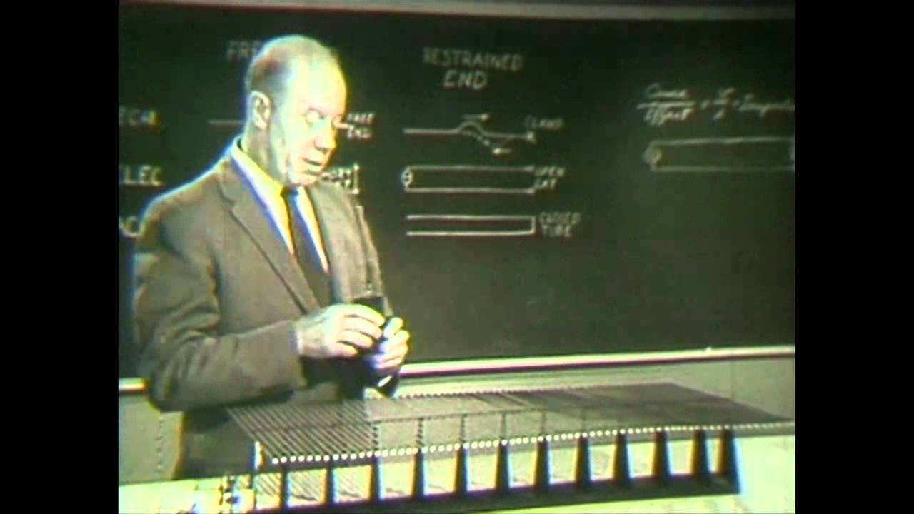
AT&T Archives: Similiarities of Wave Behavior (Bonus Edition) — AT&T Tech Channel

AT&T Tech Channel

Because waves of all kinds behave fundamentally alike, mastering mechanical wave analogies allows scientists and engineers to solve complex propagation and impedance-matching problems across electrical, acoustic, and optical systems.

AI-assisted summary of AT&T Archives: Similiarities of Wave Behavior (Bonus Edition) — original source. Check the original for full context.

Source published:

Key ideas

  • Dr. John Shive uses his custom torsional wave machine to demonstrate that wave dynamics follow identical mathematical rules across mechanical, electrical, acoustical, and optical domains. (0:00)
  • Boundary terminations determine reflection phase: rigid or clamped ends cause a 180-degree inverted reflection, whereas unrestrained free ends reflect the wave right side up with zero phase change. (3:23)
  • Standing wave ratio (SWR) measurements allow direct calculation of energy loss at mismatched terminations using electrical transmission formulas adapted for mechanical systems. (14:00)
  • Impedance discontinuities between different transmission media can be eliminated either using narrow-band quarter-wave sections or broadband tapered transitions, mirroring optical anti-reflective coatings and acoustic megaphones. (22:02)

Detailed notes

## Background Published on YouTube by the AT&T Tech Channel on April 3, 2012, this archival release presents a classic 1959 Bell Labs educational film hosted by Dr. John N. Shive. The presentation highlights Shive using his own mechanical invention—the Shive wave machine—to explain universal wave behaviors, spanning wave reflections, superposition, standing waves, resonance, and impedance matching across physical disciplines.

## TL;DR Dr. John Shive utilizes custom torsional wave machines to demonstrate that mechanical, electrical, acoustic, and optical waves operate under identical physical principles. Through methodical physical experiments, he illustrates phase inversion at clamped boundaries, non-inverted reflections at free ends, superposition cancellation, and resonance tuning. Shive introduces wave impedance by showing how dashpot terminations absorb wave energy or create partial reflections measurable via the standing wave ratio (SWR). Finally, he shows how quarter-wave sections and tapered transformers eliminate reflections at boundary discontinuities, connecting the mechanics to camera lens coatings, megaphones, and the mammalian middle ear.

## Atmosphere & style The presentation carries the poised, deliberate clarity of mid-century scientific education, propelled by Dr. Shive's articulate, unhurried lecturing style. Watching the mechanical rib crossarms twist, reflect, and cancel in rhythmic real-time motion makes invisible mathematical wave equations tangible and hypnotic. The tone is deeply earnest and intellectually cohesive, generating quiet wonder as simple mechanical vibrations seamlessly bridge into acoustics, electrical circuits, and modern optical engineering.

## Bulletin - [00:00](https://www.youtube.com/watch?v=DovunOxlY1k&t=0s) Dr. John Shive uses his custom torsional wave machine to demonstrate that wave dynamics follow identical mathematical rules across mechanical, electrical, acoustical, and optical domains. - [03:23](https://www.youtube.com/watch?v=DovunOxlY1k&t=203s) Boundary terminations determine reflection phase: rigid or clamped ends cause a 180-degree inverted reflection, whereas unrestrained free ends reflect the wave right side up with zero phase change. - [14:00](https://www.youtube.com/watch?v=DovunOxlY1k&t=840s) Standing wave ratio (SWR) measurements allow direct calculation of energy loss at mismatched terminations using electrical transmission formulas adapted for mechanical systems. - [22:02](https://www.youtube.com/watch?v=DovunOxlY1k&t=1322s) Impedance discontinuities between different transmission media can be eliminated either using narrow-band quarter-wave sections or broadband tapered transitions, mirroring optical anti-reflective coatings and acoustic megaphones.

## Key takeaways - [00:00](https://www.youtube.com/watch?v=DovunOxlY1k&t=0s) Waves across mechanical, electrical, acoustical, and optical environments share identical underlying physical behaviors. - [02:14](https://www.youtube.com/watch?v=DovunOxlY1k&t=134s) The Shive wave machine translates torsional stress along a central steel wire into observable transverse vertical motion via perpendicular crossarms. - [02:14](https://www.youtube.com/watch?v=DovunOxlY1k&t=134s) Reducing the length and rotational inertia of crossarms increases wave propagation speed along the medium by approximately three times. - [03:23](https://www.youtube.com/watch?v=DovunOxlY1k&t=203s) A clamped boundary reflects an incident pulse inverted (upside down), mirroring an electrical open circuit or a rigid acoustic wall. - [03:23](https://www.youtube.com/watch?v=DovunOxlY1k&t=203s) A free boundary reflects an incident pulse right side up, mirroring an electrical short circuit or an open acoustic tube. - [06:09](https://www.youtube.com/watch?v=DovunOxlY1k&t=369s) The principle of superposition dictates that overlapping wave amplitudes combine algebraically, allowing identical positive and negative pulses to cancel completely at the point of overlap. - [06:09](https://www.youtube.com/watch?v=DovunOxlY1k&t=369s) Continuous wave trains interfering with their own reflections produce standing waves with stationary nodes separated by exactly one-half wavelength. - [08:42](https://www.youtube.com/watch?v=DovunOxlY1k&t=522s) Resonance occurs when the round-trip travel time of a wave is an integer multiple of the drive period, building abnormal amplitude until input energy equals internal frictional loss. - [10:36](https://www.youtube.com/watch?v=DovunOxlY1k&t=636s) Wave impedance represents the ratio of cause to effect, defined mechanically as applied torque over resulting angular velocity. - [12:57](https://www.youtube.com/watch?v=DovunOxlY1k&t=777s) A fluid dashpot matched to the characteristic impedance of the wave machine absorbs all incident wave energy, eliminating reflected waves entirely. - [14:00](https://www.youtube.com/watch?v=DovunOxlY1k&t=840s) Impedance mismatch creates partial reflection, which can be evaluated by measuring the standing wave ratio (A_max / A_min) to determine the percentage of reflected energy. - [19:03](https://www.youtube.com/watch?v=DovunOxlY1k&t=1143s) Abrupt transitions between media of different impedances cause reflection and refraction, directly analogous to light crossing from glass into air. - [22:02](https://www.youtube.com/watch?v=DovunOxlY1k&t=1322s) A quarter-wave matching section neutralizes boundary reflections for continuous periodic waves, functioning identically to non-reflective camera lens coatings. - [24:02](https://www.youtube.com/watch?v=DovunOxlY1k&t=1442s) Tapered impedance transformers provide broadband matching capable of transmitting isolated pulses without reflective loss, as seen in acoustic megaphones and microwave waveguides. - [24:02](https://www.youtube.com/watch?v=DovunOxlY1k&t=1442s) Biological systems, such as the mammalian middle ear ossicles, employ mechanical impedance matching to transfer sound energy from air into cochlear fluid efficiently.

## Detailed walkthrough ### [00:00](https://www.youtube.com/watch?v=DovunOxlY1k&t=0s) Introduction to Dr. John Shive and the Wave Machine

The video opens with archival framing introducing the iconic apparatus commonly seen in university physics laboratories: the Shive wave generator. Dr. John Shive developed this mechanical device at Bell Labs during the 1950s as an intuitive teaching tool designed to bridge wave mechanics across various scientific fields, ranging from electrical circuits to physical and optical spectra. The apparatus was formally introduced to the public in this 1959 film alongside an accompanying instructional text, representing Bell Labs' broader commitment to creating hands-on educational resources for budding scientists and engineers. Decades later, newly built replicas of the device remain standard classroom equipment worldwide, despite commanding prices in the hundreds of dollars.

Dr. Shive then appears on screen to begin his lecture, noting that students and researchers across physics and engineering are constantly struck by how identically waves behave across mechanical, electrical, acoustical, and optical environments. As Dr. Shive summarizes: “These similarities are due of course to the basic fact that waves of all kinds behave fundamentally alike.”

- Dr. John Shive invented the phototransistor in 1950 and created the wave machine in the 1950s at Bell Labs. - The 1959 film was produced directly by Bell Labs to clarify abstract wave phenomena through concrete visualization.

[02:14](https://www.youtube.com/watch?v=DovunOxlY1k&t=134s) Mechanical Demonstration Apparatus Mechanics

Dr. Shive introduces two distinct, rib-like mechanical wave machines mounted in bearing assemblies that permit free rotation. The primary apparatus transmits waves via torsional strain: an initial disturbance twists a central steel wire along its longitudinal axis. Cross arms attached perpendicular to the central wire translate this torsional motion into visible transverse, vertical displacements at their outer tips.

Alongside the primary machine sits a second wave machine built on the exact same physical principles, but fitted with cross arms that are significantly shorter. Because of the reduced rotational inertia of these shorter arms, waves propagate along the second machine approximately three times faster than along the first. While both machines will later be coupled together, Dr. Shive begins his demonstrations using only the long-arm unit.

```mermaid flowchart LR accTitle: Mechanical Wave Machine Operation accDescr: Flow diagram showing how input torque converts to visible transverse motion. subgraph Input["Drive Mechanism"] A["Applied Torque"] --> B["Central Steel Wire"] end subgraph Propagation["Wave Transmission"] B --> C["Torsional Twist Propagates"] C --> D["Rigid Cross Arms"] end subgraph Output["Visual Wave"] D --> E["Transverse Up/Down Tip Motion"] end ```

[03:23](https://www.youtube.com/watch?v=DovunOxlY1k&t=203s) Total Reflection at Free and Clamped Terminations

Dr. Shive demonstrates the two fundamental ways a traveling wave reflects at a physical boundary: from an unrestrained free end and from a clamped boundary. When the final cross arm is left completely unobstructed, an upward pulse launched down the wire reaches the end, reflects, and travels backward right side up as a faithful replica of the incident pulse. Next, he locks the final cross arm tightly to a heavy stand, preventing any displacement. When an identical upward pulse strikes this immobilized end, it reflects upside down, inverting its phase completely while retaining total energy.

Dr. Shive draws analogies across several branches of physics, proving that wave physics adheres to a unified rule set regardless of the physical medium. In mechanical systems, displacement is restrained by a physical clamp; in electrical transmission lines, an open circuit stops the flow of current; and in acoustic tubes, a rigid wall terminates the longitudinal vibration of air molecules. All three clamped equivalents cause an inverted (upside-down) reflection. Conversely, a free mechanical end, an electrical short circuit (allowing free current displacement), and an open acoustic tube reflect the traveling wave right side up without phase inversion.

As Dr. Shive observes of this broad physical symmetry: “Now if Nature has any consistency and we like to think she does this alternative reflection possibility should exist for waves of all kinds and these other drawings here show that indeed it does.”

| Medium | Fixed/Clamped Boundary (Inverted / Upside Down) | Free Boundary (Erect / Right Side Up) | |:--- |:--- |:--- | | **Mechanical** | Clamped end (zero displacement) | Free end (unconstrained cross arm) | | **Electrical** | Open circuit (zero current flow) | Short circuit (unrestrained current) | | **Acoustical** | Rigidly closed tube end (zero air vibration) | Open tube end (free acoustic expansion) |

[06:09](https://www.youtube.com/watch?v=DovunOxlY1k&t=369s) Superposition and Continuous Wave Interference

Turning to the principle of superposition, Dr. Shive demonstrates what occurs when two wave pulses travel in opposite directions along the same medium simultaneously. Shown in slow motion, the two pulses pass through one another cleanly; the momentary displacement of the medium at any point is simply the algebraic sum of the individual component amplitudes. When an upright positive pulse meets an inverted negative pulse of equal shape, they cancel each other out completely at the exact instant of coincidence, leaving the medium looking completely undisturbed for a fraction of a second before each pulse emerges intact on the opposite side.

Dr. Shive then replaces single manual pulses with a continuous periodic train of waves generated by an electric motor and crank mechanism mounted at the input end. When these waves reflect continuously off the far terminal, oncoming waves continuously superpose onto the reflected waves traveling back. This produces a classic standing wave pattern. Rather than traveling horizontally along the central wire, the segments of the medium simply bob up and down in place. Between these oscillating segments sit completely stationary points called nodes, spaced precisely one-half wavelength apart, just like the vibrational modes of a musical string.

- Superposition principle: resultant amplitude equals the exact algebraic sum of individual wave amplitudes at every instant. - Complete destructive cancellation occurs during the mutual overlap of equal positive and negative pulses. - Standing wave nodes (points of absolute rest) are separated by distances of exactly $\frac{1}{2}\lambda$.

[08:42](https://www.youtube.com/watch?v=DovunOxlY1k&t=522s) Resonance, Tuning, and Energy Storage

Dr. Shive demonstrates how standing waves transition into resonance by adjusting the physical length of the line. By sliding the reflective end bracket slightly toward the motorized crank, he adjusts the line length so that the round-trip travel time of a wave is an exact integer multiple of the motor's wave period. In this tuned condition, every newly launched crest arrives at precisely the right phase to reinforce previously reflected waves.

As Dr. Shive explains: “Under these conditions the new waves which are continually being sent out by the generator superpose upon the previously emitted and multiply reflected waves in just the right phase to build up the amplitude to an abnormally large value new Crest on previous Crest and so on.”

The wave machine enters violent, high-amplitude resonance, reaching an equilibrium state where the input energy supplied by the motor per cycle matches the energy lost to internal friction. Dr. Shive points out that this state of resonance could equally be attained by keeping the machine's length fixed and adjusting the generator's drive frequency instead. Altering either the length or the drive frequency by even a small amount instantly collapses the resonance pattern. He highlights that resonant assemblies act fundamentally as energy reservoirs, citing the balance escapement wheel of a mechanical watch, a child swinging on a playground swing, an organ pipe, and the LC tank circuit of a radio transmitter as identical physical embodiments of resonance.

```mermaid flowchart TD accTitle: Mechanics of Resonance accDescr: Step-by-step diagram illustrating the conditions and outcome of wave resonance. A["Motor Drive Launches Periodic Wave"] --> B["Wave Reflects at Terminus"] B --> C{"Round-Trip Travel Time = Multiple of Period?"} C -- "No (Untuned)" --> D["Irregular Low-Amplitude Interference"] C -- "Yes (Tuned)" --> E["In-Phase Crest-on-Crest Superposition"] E --> F["Resonant Amplitude Multiplies"] F --> G["Steady State: Input Energy = Friction Loss"] ```

[10:36](https://www.youtube.com/watch?v=DovunOxlY1k&t=636s) Concept of Impedance and Load Matching

Transitioning to wave impedance, Dr. Shive explains that launching waves along any transmission line involves two distinct variables: an originating cause and a resulting effect. While students encounter the concept most often in electrical circuits—where an alternating input voltage acts as the cause and the resulting alternating current acts as the effect—the exact same relationship defines mechanical wave systems. In the torsional wave machine, the cause is the oscillating torque applied to the input cross arm, while the effect is the resulting angular velocity of the structure. Mechanical impedance is the ratio of that applied torque to the resulting angular velocity.

Dr. Shive notes that when transmitting signals down a line, engineers usually aim to terminate the line with an impedance that exactly matches the characteristic impedance of the medium itself. When a terminating load matches the line impedance, it absorbs all incoming wave energy, eliminating reflections entirely. To demonstrate this experimentally, he brings out a mechanical dashpot termination consisting of a small water-filled tin can and an internal damper piston attached to the final cross arm.

- Electrical impedance: $\frac{\text{Voltage (cause)}}{\text{Current (effect)}}$. - Mechanical impedance: $\frac{\text{Applied Torque (cause)}}{\text{Angular Velocity (effect)}}$. - Impedance matching: adjusting the terminating load to match the transmission medium so 100% of the wave energy is absorbed with zero reflected wave.

[12:57](https://www.youtube.com/watch?v=DovunOxlY1k&t=777s) Dashpot Termination and Impedance Matching

Dr. J.N. Shive demonstrates how an absorbing termination can eliminate wave reflection at the end of the line. The apparatus uses a dashpot with a plunger pumping up and down in damping fluid. By sliding the dashpot inward or outward along the final crossarm of the wave machine, Dr. Shive adjusts the counter-torque with which the device resists the displacement of the medium. Through this physical adjustment, he matches the mechanical impedance of the dashpot to the characteristic impedance of the transmission line itself.

When the adjustment is correctly calibrated, the dashpot absorbs the incoming wave energy completely, preventing any noticeable rebound. Dr. Shive tests this first with isolated single pulses and then engages a continuous wave train. The waves travel down the machine from the generator end to the load end, disappearing smoothly into the dashpot without reflecting. As Dr. Shive explains: “When this adjustment is properly made, the dashpot absorbs all the wave energy that travels down the line and as you can see hardly any perceptible reflection takes place.”

- Sliding the dashpot along the crossarm alters the counter-torque lever arm to match the transmission line's mechanical impedance. - With matched impedance, single wave pulses and continuous wave trains are fully absorbed at the termination.

[14:00](https://www.youtube.com/watch?v=DovunOxlY1k&t=840s) Partial Reflection, SWR, and Calculating Energy Loss

Dr. Shive intentionally spoils this balanced condition by sliding the dashpot inward toward the central wire, reducing the load impedance below that of the transmission line. When continuous waves are driven down the system, the mismatched termination creates a partial reflection. Forward-propagating waves and reflected waves of identical frequency share the medium simultaneously, but because the returning wave possesses a smaller amplitude, the resulting interference differs fundamentally from total reflection. While stationary nodes appeared under 100% reflection from a clamped end, this partial reflection produces nodes that do not stand completely still; instead, the entire wave envelope fluctuates between fixed upper and lower limits.

```mermaid flowchart LR accTitle: Standing Wave Ratio and Percent Reflection Workflow accDescr: Process of measuring maximum and minimum envelope amplitudes to determine SWR and total reflected power. subgraph S1["Envelope Measurement"] A["Forward & Reflected Waves"] --> B["Standing Wave Envelope"] B --> C["A_max = 5 units<br/>A_min = 2 units"] end subgraph S2["SWR Calculation"] C --> D["SWR = A_max / A_min<br/>SWR = 5/2 = 2.5"] end subgraph S3["Reflection Percentage"] D --> E["Reflection Formula:<br/>((SWR - 1)/(SWR + 1))^2 * 100"] E --> F["Result: 9/49 ≈ 18% Reflected Energy"] end ```

By speeding up the film footage, Dr. Shive reveals the complete envelope profile, characterized by an amplitude maximum ($A_{\text{max}}$) and an amplitude minimum ($A_{\text{min}}$). In wave theory, the ratio of $A_{\text{max}}$ to $A_{\text{min}}$ is defined as the standing wave ratio (abbreviated SWR). On his wave machine, this ratio measures approximately 3:1. When the end was clamped for total reflection, motionless nodes produced an SWR of infinity; conversely, under a perfect match, $A_{\text{max}}$ equaled $A_{\text{min}}$, yielding an SWR of unity. Dr. Shive underscores the practical utility of this relationship: “The punchline is this: in any practical case of reflection, a measurement of the standing wave ratio on the medium just ahead of the termination enables one to calculate the percent reflection that is taking place there.”

Using a pair of identical vertical scales, Dr. Shive measures the envelope live on the machine, reading an $A_{\text{max}}$ of 5 units and an $A_{\text{min}}$ of 2 units, establishing an SWR of $\frac{5}{2}$. He substitutes this value into the percent reflection formula:

$$\% \text{ Reflection} = \left(\frac{\text{SWR} - 1}{\text{SWR} + 1}\right)^2 \times 100 = \left(\frac{\frac{5}{2} - 1}{\frac{5}{2} + 1}\right)^2 \times 100 = \left(\frac{\frac{3}{2}}{\frac{7}{2}}\right)^2 \times 100 = \frac{9}{49} \times 100 \approx 18\%$$

Dr. Shive highlights the conceptual unity across physics: “Now this is a perfectly valid and logical thing for me to do since waves of all kinds behave alike.”

- Clamped termination: 100% reflection, motionless nodes, $\text{SWR} = \infty$. - Matched termination: 0% reflection, no standing wave pattern, $A_{\text{max}} = A_{\text{min}}$, $\text{SWR} = 1$. - Measured partial reflection values: $A_{\text{max}} = 5$, $A_{\text{min}} = 2$, yielding $\text{SWR} = 2.5$ and approximately $18\%$ energy reflected. - The formula originated in alternating-current electrical engineering but applies universally to mechanical, acoustic, and electromagnetic systems.

[19:03](https://www.youtube.com/watch?v=DovunOxlY1k&t=1143s) Impedance Discontinuities Between Coupled Media

Dr. Shive introduces a second core principle: wave reflections occur not only at improper end terminations, but whenever a wave encounters an abrupt change in the transmission medium itself. To demonstrate this, he joins two separate wave machines end-to-end, securing their central torsion wires together with a small clamp. The combined setup forms a single transmission path comprising two sections with distinct mechanical impedances.

A wave traveling slowly along the first machine accelerates abruptly upon crossing the central junction into the second machine, mirroring the refraction and reflection of a light beam emerging from glass into air. To isolate the junction and prevent spurious reflections from the far boundary, Dr. Shive secures a matched dashpot at the far terminal end. He sends single pulses down the line, prompting the audience to watch closely as the primary wave passes the midpoint: a distinct reflected pulse rebounds backward toward the source from the central clamp.

When the motorized continuous wave generator is engaged, this mid-line junction creates a persistent partial standing wave pattern on the input section. Dr. Shive observes that calculating the maximum and minimum envelope amplitudes yields the energy lost to reflection at any interface discontinuity, noting: “Electric waves, light waves, sound waves, mechanical waves are partly reflected when they encounter impedance discontinuities.”

- Coupling two machines with different crossarm dimensions creates an abrupt impedance mismatch at the clamped joint. - Waves crossing the boundary change propagation speed, replicating optical transmission across a glass-air interface. - Reflected energy forms a standing wave envelope upstream of the interface, which can be evaluated using the SWR formula.

[22:02](https://www.youtube.com/watch?v=DovunOxlY1k&t=1322s) Quarter-Wave Matching Transformers and Optical Coatings

In practical engineering systems, partial reflections caused by impedance discontinuities represent an unwelcome waste of energy. To eliminate these losses, engineers interpose impedance-matching devices between mismatched media. Dr. Shive exhibits a mechanical quarter-wave matching transformer: a specialized section of wave medium exactly one quarter-wavelength ($\frac{\lambda}{4}$) in length, featuring crossarms whose length is intermediate between the dimensions of the two primary machines.

Dr. Shive sandwiches this quarter-wave section into the junction between the two transmission lines. When continuous waves are driven through the combined assembly, wave energy passes smoothly across the boundary into the second machine without reflection. The partial standing wave envelope on the input line disappears entirely, proving that the impedances have been coupled seamlessly.

He connects this mechanical apparatus directly to camera technology: “The non-reflecting coating on the lens of this camera is an optical quarter-wave matching transformer; it works in precisely the same way with light waves.” However, Dr. Shive acknowledges two significant limitations inherent to the quarter-wave design: 1. It functions solely for continuous, periodic waves. 2. It operates efficiently only within a narrow frequency band centered on the exact wavelength for which the section was dimensioned.

[24:02](https://www.youtube.com/watch?v=DovunOxlY1k&t=1442s) Broadband Tapered Transformers and Universal Wave Principles

To circumvent the narrow bandwidth and continuous-wave limitations of quarter-wave transformers, acoustic, mechanical, and radio engineers rely on tapered sections. Dr. Shive holds up an ordinary acoustic megaphone as an intuitive example: the megaphone smooths the impedance discontinuity between the high-impedance air column inside the human throat and mouth and the low-impedance free air of the surrounding room by means of a continuous, gradual flare.

Applying this geometry to his apparatus, Dr. Shive inserts a mechanical tapered section whose crossarms gradually transition from the width of the input machine to the width of the output machine. Unlike the quarter-wave section, this tapered transformer operates across a wide frequency band and accommodates single transient pulses. Dr. Shive transmits sharp, narrow pulses and longer wave pulses through the assembly; in both instances, energy transfers across the interface with virtually no perceptible reflection.

Dr. Shive expands on the ubiquity of impedance matching throughout technology and biology: - **Microwave engineering:** Tapered waveguide sections smoothly join rectangular waveguides of different dimensions to prevent reflective radiation loss. - **Electrical power:** Transformers span extremes of scale, ranging from tiny circuit components to house-sized units in hydroelectric power plants. - **Biology:** The mammalian middle ear employs three tiny bones—the malleus (hammer), incus (anvil), and stapes (stirrup)—as a mechanical linkage to match the low impedance of airborne sound in the outer ear to the high impedance of fluid within the inner ear cochlea. - **Unidirectional mechanics:** Classical machines providing mechanical advantage—such as gear trains, levers, and block-and-tackle pulley systems—act as impedance-transforming devices for unidirectional work.

Reflecting on these diverse demonstrations, Dr. Shive articulates the overarching theme of the lecture: “One thing that has always profoundly impressed me is this: waves of all kinds behave alike.”

- Megaphones provide acoustic impedance tapering from the vocal tract to open air. - Tapered transmission lines handle pulses and broad frequency spectra without narrowband tuning constraints. - The middle ear ossicles act as an impedance-matching transformer between air and cochlear liquid. - Simple machines (levers, pulleys, gear trains) serve as impedance converters for steady mechanical forces.

[27:11](https://www.youtube.com/watch?v=DovunOxlY1k&t=1631s) Understanding Wave Behavior Across Disciplines

Dr. J.N. Shive concludes his presentation by reflecting on the broad, unifying power of wave mechanics. Whether an individual approaches this subject through a specialized field where wave phenomena happen to play a central role, or pursues the study of wave dynamics purely for its own sake, gaining this foundational knowledge equips a scientist or engineer with universal conceptual tools.

Shive emphasizes that mastering these core mechanical analogies allows one to move fluidly between seemingly unrelated technical domains. As he summarizes the ultimate takeaway of his lecture: “...of some discipline in which waves play an important role or even through the study of waves for themselves alone then you will always feel at home in any branch of physics or engineering where the main show has to do with waves and how they behave.”

## Notable quotes > [19:03](https://www.youtube.com/watch?v=DovunOxlY1k&t=1143s) Electric waves, light waves, sound waves, mechanical waves are partly reflected when they encounter impedance discontinuities. — Dr. J.N. Shive

> [24:02](https://www.youtube.com/watch?v=DovunOxlY1k&t=1442s) One thing that has always profoundly impressed me is this: waves of all kinds behave alike. — Dr. J.N. Shive

> [14:00](https://www.youtube.com/watch?v=DovunOxlY1k&t=840s) The punchline is this: in any practical case of reflection, a measurement of the standing wave ratio on the medium just ahead of the termination enables one to calculate the percent reflection that is taking place there. — Dr. J.N. Shive

## Mentioned Dr. John Shive, Bell Labs, Shive Wave Machine, AT&T Archives

## Video description For more from the AT&T Archives, visit http://techchannel.att.com/archives

On an elementary conceptual level, this film reflects the multifaceted scientific hyperthinking that was typical of a Bell Labs approach. Host Dr. J.N. Shive's presence as a lecturer is excellent - it's understandable by a layperson even when he branches into equations, because he uses copious amounts of real-world examples to bolster the material.

Shive's role at Bell Labs was more than just a great lecturer: he worked on early transistor technology, inventing the phototransistor in 1950, and the machine he uses in the film is his invention, now called the Shive Wave Machine in college classrooms.

Dr. J.N. Shive of Bell Labs demonstrates and discusses the following aspects of wave behavior:

Reflection of waves from free and clamped ends Superposition Standing waves and resonance Energy loss by impedance mismatching Reduction of energy loss by quarter-wave and tapered-section transformers Original audience: college students

Produced at Bell Labs

Footage courtesy of AT&T Archives and History Center, Warren, NJ

[Source](https://www.youtube.com/watch?v=DovunOxlY1k)

中文简报

贝尔实验室工程师约翰·夏夫借助新机器统一波动物理学 由于各类波的行为从本质上均相似,掌握机械波类比使科学家和工程师能够解决电学、声学和光学系统中复杂的传播与阻抗匹配问题。 约翰·夏夫博士利用定制的扭转波机器证明,机械波、电磁波、声波和光波均遵循相同的物理原理。通过系统性的物理实验,他展示了固定端的相位反转、自由端的同相反射、叠加相消以及共振调谐。夏夫还通过展示阻尼器末端如何吸收波能量或产生可通过驻波比(SWR)测量的部分反射,引出了波阻抗的概念。最后,他演示了四分之一波长段和渐变变压器如何消除边界不连续处的反射,将力学原理与相机镜头镀膜、扩音器以及哺乳动物的中耳联系起来。 约翰·夏夫博士利用其定制的扭转波机器证明,波动力学在力学、电学、声学和光学领域遵循完全相同的数学规律。 (0:00) 边界终端决定反射相位:刚性或固定端会引起180度的倒相反射,而无约束的自由端则会以零相位变化实现同相反射。 (3:23) 利用适用于机械系统的电传输公式,驻波比(SWR)测量可以直接计算失配终端处的能量损失。 (14:00) 不同传输介质之间的阻抗不连续性既可以通过窄带四分之一波长段消除,也可以通过宽带渐变过渡段消除,这与光学增透膜和声学扩音器的原理如出一辙。 (22:02)

Reading summary

Dr. John Shive demonstrates that waves across mechanical, electrical, acoustical, and optical systems behave identically, sharing unified physical rules for reflection, resonance, and impedance matching. Boundary Reflection Symmetries Across Media (3:23) Using a torsional wave machine composed of a central steel wire and perpendicular cross arms, Dr. Shive demonstrates that boundary reflections follow universal symmetry rules. A wave pulse traveling to an unrestrained, free end reflects right side up without phase inversion. Conversely, when the terminal cross arm is locked to prevent displacement, an incoming upward pulse reflects inverted, inverting its phase completely while returning its full energy back into the line. Shive maps this behavior directly to other physical domains. In electrical transmission lines, an open circuit stops current flow and acts as a clamped boundary that inverts reflection, whereas a short circuit permits unrestrained current and reflects right side up. In acoustics, a rigid wall closing a tube stops air vibration to cause an inverted reflection, while an open tube end permits unconstrained acoustic expansion and preserves the wave's orientation. Superposition, Standing Waves, and Resonant Storage (6:09) When multiple wave pulses share a medium simultaneously, they follow the principle of superposition: the net displacement at any point equals the algebraic sum of the individual component amplitudes. Opposing pulses pass through each other cleanly, with equal positive and negative pulses momentarily canceling each other entirely at their point of coincidence. Applying continuous periodic waves against a reflective terminus produces standing waves, where oncoming and reflected waves superpose into oscillating segments separated by stationary nodes spaced exactly one-half wavelength apart. When line length or generator frequency is tuned so the round-trip travel time equals an exact integer multiple of the wave period, the system enters resonance. In this state, input waves reinforce reflected waves in phase to amplify energy until input power matches frictional losses, operating as an energy reservoir comparable to radio LC tank circuits, organ pipes, or watch balance wheels. Impedance Matching and Reflection Calculations (10:36) Wave impedance is defined across disciplines as the ratio of originating cause to resulting effect. In electrical lines, this is alternating voltage divided by alternating current; in Shive's mechanical wave machine, it is applied torque divided by angular velocity. Terminating a transmission medium with a load that matches its characteristic impedance—such as an adjustable fluid dashpot calibrated to supply equal counter-torque—absorbs all wave energy and prevents reflections entirely. When terminal impedance is mismatched, partial reflections occur, producing a standing wave envelope whose nodes fluctuate between an amplitude maximum and minimum. Shive measures the standing wave ratio (SWR), defined as maximum amplitude divided by minimum amplitude. Testing an SWR of 2.5 (5 units over 2 units), Shive applies the electrical engineering formula ((SWR - 1) / (SWR + 1))^2 * 100 to calculate that approximately 18% of the wave energy is reflected, proving the formula's universal mechanical validity. Narrowband and Broadband Impedance Transformers (22:02) Reflections occur not only at terminations but wherever a wave encounters an abrupt change in the transmission medium, analogous to light refracting and reflecting when moving from glass into air. Coupling two wave machines with different cross-arm lengths creates an impedance discontinuity that reflects a portion of the incoming energy back toward the source. To bridge media without energy loss, engineers employ transformers. A mechanical quarter-wavelength matching section with intermediate dimensions completely eliminates reflections, functioning identically to non-reflective optical coatings on camera lenses; however, this mechanism is restricted to continuous periodic waves within a narrow frequency band. To handle transient pulses and wide frequency ranges, tapered sections provide a gradual transition, exemplified by acoustic megaphones, tapered microwave waveguides, mammalian middle ear ossicles coupling airborne sound to cochlear fluid, and unidirectional mechanical systems like levers and gear trains. Dr. Shive concludes that mastering foundational wave mechanics and impedance relationships through concrete analogies allows researchers and engineers to move fluidly between seemingly unrelated fields of physics and engineering.

精炼阅读摘要

贝尔实验室(Bell Labs)科学家 John Shive 博士通过其发明的机械扭转波浪发生器证明,机械、电学、声学和光学等不同物理介质中的波动现象遵循相同的动力学与阻抗匹配规律。 机械演示装置与边界反射规律 (3:23) Shive 博士在 1950 年代研制了由中心钢丝与刚性横臂构成的机械波发生器,施加于前端的扭矩沿钢丝以扭转应变形式传播,并由横臂末端转化为可视的横向上下位移。演示中使用了两种规格的机器:主装置横臂较长;第二台装置的横臂较短,因转动惯量较低,其波传播速度约为主装置的三倍。通过调整传输线路末端的约束条件,波在自由边界与固定边界呈现出完全不同的反射模式。当终端横臂无约束自由活动时,向上入射的脉冲反射后保持直立同相;而当终端被夹具死死固定时,脉冲发生相位翻转,以倒立形式反射并保留全部能量。 Shive 将这一边界反射规律推广至其他学科领域,指出这种对称性体现了物理法则的一致性。在机械系统中,夹紧端限制位移导致倒相反射,自由端则产生直立反射;在电路传输线中,开路切断电流流动产生倒相反射,而短路允许电流自由位移则产生直立反射;在声学管道中,刚性封闭壁面抑制空气分子振动导致倒相反射,开放管口则反射直立波。这些实验表明,波遇到边界时的相位行为不受具体传输介质的材质限制,完全由末端约束状态决定。 波的叠加原理、驻波与共振储能 (6:09) 在探讨连续波的动力学时,慢动作演示表明两列相向传播的波脉冲相遇时满足叠加原理,介质在任意点的瞬时位移严格等于各分量振幅的代数和。当形状相同但一正一负的两个脉冲完全重叠时,介质位移瞬间归零,随后两个脉冲无损穿透彼此并恢复原形。改用电动机驱动输入端产生连续周期波后,入射波与末端反射波持续叠加,形成了在原位上下振动而非水平推进的驻波图案,驻波中振幅为零的固定节点间距严格等于二分之一波长(λ/2)。 通过调节装置长度使波的往返传播时间恰好等于电动机驱动周期的整数倍,系统进入剧烈的共振状态。此时新发出的波峰与历次反射波峰完全同相叠加,使振幅急剧攀升,直至电机每周期输入的能量与系统内部摩擦损耗达到动态平衡。Shive 指出,保持长度不变而微调驱动频率也能达到相同效果,但参数稍有偏移共振即刻瓦解。他将这种共振结构定性为物理储能器,并举例指出机械手表的游丝摆轮、秋千、管风琴管以及无线电发射机中的 LC 谐振回路在物理机制上均属同类共振系统。 阻抗概念、吸收终端与驻波比计算 (10:36) 波阻抗被定义为激发波的“原因”与产生的“结果”之比值。在交流电路中,阻抗表现为电压与电流的比值;而在机械扭转波机中,阻抗则由施加的扭矩(原因)除以产生的角速度(结果)决定。当传输线终端负载的阻抗与介质本身的特性阻抗完全匹配时,负载能完全吸收波能量而不产生反射。Shive 采用由充水罐和连接在末端横臂上的阻尼活塞组成的减震器(dashpot)进行验证,通过沿横臂向内或向外滑动减震器改变反向扭矩力臂,成功调谐出与波浪机特性阻抗一致的状态,使单脉冲与连续波列均无反射平滑消失于终端。 若人为破坏平衡,将减震器向内滑动降低负载阻抗,失配终端就会产生部分反射。由于反射波振幅小于前向波,二者干涉形成的驻波包络节点不再完全静止,而是在最大振幅(A_max)与最小振幅(A_min)之间起伏。此时 A_max 与 A_min 的比值即为驻波比(SWR)。在现场测量中,读取到 A_max 为 5 个单位、A_min 为 2 个单位,计算得 SWR 为 2.5。代入源自交流电工程的反射能量公式 [(SWR - 1)/(SWR + 1)]^2 × 100,得出该失配边界反射了约 18% 的波能量。相比之下,完全反射时 SWR 为无穷大,完全匹配时 SWR 为 1。 介质不连续性与阻抗变换器的工程应用 (19:03) 反射不仅发生在末端终端,当波遭遇介质突变时同样会发生部分反射。Shive 将横臂长度不同的两台波浪机通过中心钢丝夹紧串联,使行波从慢速介质穿入快速介质,其过程类似于光线由玻璃进入空气。单波脉冲通过交界面时,一部分能量越过接头加速传播,另一部分能量则作为反射波折返源头,并在输入段产生持续的部分驻波包络。为了消除这种由界面阻抗不连续性引起的能量浪费,工程上广泛采用阻抗变换器件。 Shive 首先展示了机械四分之一波长变换器(λ/4),其截面长度精确为波长的四分之一,横臂长度介于两机之间。将该段夹在两机中间后,连续波无反射顺利通过,输入端的驻波包络完全消失。Shive 指出照相机镜头上的防反射涂层即是光学四分之一波长匹配器,但该结构仅适用于连续波且带宽较窄。为克服这一缺陷,工程中引入渐变过渡段(tapered section)。例如普通声学扩音喇叭利用逐渐张开的号筒平滑过渡人喉高阻抗与空气低阻抗;机械渐变装置同样实现了宽频带和单脉冲的无反射过渡。这一阻抗匹配机制在自然界与工业中极为普遍:微波工程采用渐变波导管防止辐射反射;电力系统依靠变压器进行阻抗转换;哺乳动物中耳的三块听小骨将外耳空气的低阻抗转换为内耳耳蜗液的高阻抗;杠杆、滑轮组与齿轮系统也是用于单向机械功的阻抗变换工具。 Shive 总结指出,跨学科的波动行为在数学和物理机制上具有根本的统一性;无论是专精某一具体应用领域还是探索波动理论本身,掌握基于阻抗和波动动力学的核心机械类比模型,都能使科研人员和工程师迅速理解并处理声、光、电及机械工程中各类复杂的波现象。

Detailed notes — zh

## Background 该视频由 AT&T Tech Channel 于 2012 年 4 月 3 日发布在 YouTube 平台上,取材自 1959 年贝尔实验室制作的经典科学典藏影像。页面简介介绍,影片由光电晶体管发明者约翰·沙夫博士(Dr. J.N. Shive)主讲,他使用自己发明的“沙夫波动发生器”向大学物理学生直观演示波动的全反射、叠加、驻波共振、阻抗失配能量损失以及四分之一波长与渐变变压器匹配等核心概念。 ## TL;DR 沙夫博士借助其发明的扭转机械波演示机,生动揭示了机械波、电磁波、声波和光波之间深刻的内在统一性。他系统演示了自由端与固定端的全反射差异、叠加原理下的波形抵消,以及连续波叠加形成的驻波与系统共振。随后,沙夫深入探讨了介质阻抗的本质,通过调节阻尼器展示了阻抗失配带来的部分反射,并利用交流电学公式现场计算驻波比(SWR)。最后,他展示了如何利用四分之一波长变压器和渐变截面变压器消除反射损耗,并将这一机制延伸至相机增透膜、喇叭扩音器以及哺乳动物听小骨等工程与生物学实例。 ## Atmosphere & style 整部影片散发着 20 世纪中期贝尔实验室标志性的严谨、纯粹与从容不迫的科学美感。沙夫博士仪表端庄、讲学神态自信且极具亲和力,他用最质朴的机械装置、手持刻度尺和黑板板书,将抽象艰深的波动微分方程转化为肉眼可见的优雅物理运动。镜头在黑白胶片的慢动作特写与全景推拉间切换,没有现代花哨的特效剪辑,只有规律起伏的金属骨架与清脆的机械声,带给观众一种在物理世界底层逻辑中穿梭的沉静与震撼。 ## Bulletin - [00:00](https://www.youtube.com/watch?v=DovunOxlY1k&t=0s) 沙夫波动发生器由贝尔实验室物理学家约翰·沙夫博士于20世纪50年代发明,通过中心金属丝的扭转波与横臂的横向运动,将电学、声学与光学的波动行为具象化为机械模型。 - [03:23](https://www.youtube.com/watch?v=DovunOxlY1k&t=203s) 波在介质末端反射的形式由终端约束决定:自由端产生同向正立反射,而固定约束端则导致波形完全反转倒立,该规律在机械波、电气传输线及声学管道中完全通用。 - [15:32](https://www.youtube.com/watch?v=DovunOxlY1k&t=932s) 借助阻尼缓冲器消除末端反射并构建驻波,沙夫利用交流电学中的驻波比(SWR)公式现场测算,验证了机械波部分驻波图样中约18%的能量反射率。 - [22:02](https://www.youtube.com/watch?v=DovunOxlY1k&t=1322s) 针对介质交界处的阻抗突变与反射损失,四分之一波长匹配变压器可精准消除特定窄带连续波的反射(类似镜头增透膜),而渐变截面变压器则能实现宽频带范围内的无反射平滑过渡。 ## Key takeaways - [01:48](https://www.youtube.com/watch?v=DovunOxlY1k&t=108s) 不同物理领域的波动行为具有高度内在一致性:机械波、电磁波、声波和光波遵循相同的数学与物理规律。 - [01:48](https://www.youtube.com/watch?v=DovunOxlY1k&t=108s) 机械波演示机利用中心金属丝传播扭转波,并通过横臂将其转换为两端可见的上下横向振动;横臂尺寸决定了波在介质中的传播速度。 - [03:23](https://www.youtube.com/watch?v=DovunOxlY1k&t=203s) 末端约束条件决定全反射波形:自由端(电气短路、声学开放端)反射保持正立,固定端(电气开路、声学封闭端)反射则产生倒立反转。 - [06:15](https://www.youtube.com/watch?v=DovunOxlY1k&t=375s) 波的叠加原理严格成立:同向传播或相向传播的两个波包重叠时,介质位移为两列波瞬时振幅的代数和,异号波相遇时会瞬间完全抵消。 - [07:16](https://www.youtube.com/watch?v=DovunOxlY1k&t=436s) 正弦连续波与反射波相向叠加形成驻波,质点原地振动且空间波形不前移,相邻静止波节之间的物理间距恒等于半个波长。 - [08:42](https://www.youtube.com/watch?v=DovunOxlY1k&t=522s) 当波往返时间等于波周期的整数倍时系统进入共振,振幅大幅增加,共振系统本质上是多个周期能量累积的能量水库。 - [10:36](https://www.youtube.com/watch?v=DovunOxlY1k&t=636s) 阻抗在统一定义下为“初始起因”与“响应结果”的比值;当末端负载阻抗与传输线特征阻抗完全匹配时,波能量被全额吸收且无反射。 - [15:32](https://www.youtube.com/watch?v=DovunOxlY1k&t=932s) 末端阻抗失配会导致部分反射并形成部分驻波,其驻波比(SWR = Amax / Amin)可直接套用交流电学公式精确计算能量反射百分比。 - [18:57](https://www.youtube.com/watch?v=DovunOxlY1k&t=1137s) 介质本身特性阻抗的突变边界同样会产生能量的部分透射与部分反射,这与光线穿过玻璃与空气界面发生折射与反射的原理完全相同。 - [22:02](https://www.youtube.com/watch?v=DovunOxlY1k&t=1322s) 四分之一波长匹配变压器通过介入特定厚度介质抵消交界反射,其物理机制与光学镜头增透膜一致,但受限于狭窄频带和连续波条件。 - [24:02](https://www.youtube.com/watch?v=DovunOxlY1k&t=1442s) 渐变截面变压器提供平滑的阻抗过渡,能在宽频带下有效消除脉冲和连续波的反射,广泛应用于扩音喇叭、微波波导及变压器设备中。 - [24:02](https://www.youtube.com/watch?v=DovunOxlY1k&t=1442s) 哺乳动物耳内的三块听小骨通过杠杆结构实现外耳空气与内耳淋巴液之间的力学阻抗转换,证明了阻抗匹配原理在生物进化中的自然应用。 - [27:11](https://www.youtube.com/watch?v=DovunOxlY1k&t=1631s) 透彻掌握波动的基础规律能够建立跨学科的直觉与分析框架,帮助研究人员自由迁移应用到射频工程、声学、微波及光学等各个领域。 ## Detailed walkthrough ### [00:00](https://www.youtube.com/watch?v=DovunOxlY1k&t=0s) 贝尔实验室的波动演示仪与约翰·沙夫博士 在视频开篇,旁白指着一张老照片向观众提问,询问这一装置是否让人联想到大学物理课。照片中的设备正是“沙夫波动发生器”(Shive Wave Generator),由主讲人约翰·沙夫博士(Dr. John Shive)于 20 世纪 50 年代在贝尔实验室(Bell Labs)发明。沙夫设计这台机器的初衷,是将其作为一种教学工具,帮助学生直观理解跨学科的波动概念——涵盖从电学、力学到光谱学等诸多领域。该机器在这部 1959 年拍摄的影片中首次公开展出,并随附配套书籍发行,属于 AT&T 贝尔实验室为培养下一代科学家提供新型教学工具计划的一部分。如今,这台机器已成为全球物理课堂的标准配置;即使购买全新制造的版本,售价依然高达数百美元。旁白称赞沙夫不仅是一位发明家,更是一位极具天赋的演讲者,在这部典藏影片中充分展现了他对物理学的热爱。 - **装置名称**:沙夫波动发生器(Shive Wave Generator / Shive Wave Machine) - **发明人**:约翰·沙夫博士(Dr. John Shive),贝尔实验室物理学家,1950 年曾发明光电晶体管(Phototransistor) - **影片年份**:1959 年(由 AT&T 档案与历史中心提供) --- ### [01:48](https://www.youtube.com/watch?v=DovunOxlY1k&t=108s) 机械波机器的构造与波动共性 沙夫博士正式登场,阐述了物理学和工程学各领域中波动的内在统一性。他强调,不论是机械、电气、声学还是光学波系统,研究波动的学者都会惊叹于它们行为的高度相似。现场摆放着两台由“肋骨状”结构组成的机械波演示机,沙夫介绍说,沿着机器传播的波本质上是扭转波(torsional wave),沿着一根中心导线(central wire)传播;中心导线上固定着一根根横臂(cross arms),横臂将中心导线的扭转运动转化为两端可见的上下横向振动(transverse motion)。整个结构由一组轴承支撑,使中心金属丝能够自由扭转。 两台机器之间存在关键差异:第二台机器的横臂明显比第一台短得多。这种几何尺寸的变化直接改变了波速,第二台机器上的波速大约是第一台的 3 倍。沙夫指出,后续演示中将利用这两台不同特性的机器来展示更复杂的波动物理机制。 沙夫博士总结道:“People who study waves extensively in the various fields of physics and engineering are impressed by the similarities which exist in the behavior of waves in various mechanical, electrical, acoustical, and optical wave systems.” ```mermaid flowchart LR accTitle: 机械扭转波演示机结构 accDescr: 展示中心金属丝的扭转运动如何通过横向臂转换为两端的上下横向振动。 subgraph Machine["沙夫波动发生器机制"] A["中心金属丝 (扭转波传播)"] -->|"刚性连接带动"| B["横臂 (Cross Arms)"] B -->|"运动转换"| C["横臂末端上下横向振动"] D["支撑轴承"] -.->|"消除阻力"| A end ``` --- ### [03:23](https://www.youtube.com/watch?v=DovunOxlY1k&t=203s) 自由端与固定端的全反射:机械、电气与声学类比 沙夫演示了机械波在末端完全反射的两种截然相反的模式。首先,他保持机器末端为“自由端”(free end),即最后一根横臂没有任何束缚,可以自由运动。当一个向上的脉冲波从机器输入端发出传到末端时,反射回来的波保持完全相同的方向(正立,right side up)返回,犹如原始波形的复制品。接着,沙夫改变终端约束条件:他用重型支架将最后一根横臂牢牢夹住,使其完全无法发生位移(固定端/clamped end)。再次发射脉冲波时,反射波发生完全反转,呈现为倒立(upside down)状态反射回来。沙夫归纳道:在机械波系统中,自由端反射为正立,完全约束端反射为倒立。 为了证明“大自然是具有内在一致性(consistency)的”,沙夫将这一规律拓展到电气与声学系统,并展示了图表对比: - **电气传输线**:若终端开路(open circuit),电流被完全阻断(阻止流动),反射电压波发生反转(倒立);若终端短路(short circuit),则对应无约束情况,反射形式保持一致。 - **声学管道**:若管道末端用刚性端盖封闭(rigid closure),空气分子的纵向振动被完全遏制,反射波反转(倒立);若末端开放(声学自由端),反射波保持正立返回。 沙夫断言:“In a mechanical wave system then, there are two ways in which the total reflection of waves may take place: right side up if the reflecting end of the medium is completely free, and upside down if the reflecting end is completely restrained.” | 波动系统 | 约束端(阻止位移/流动)反射波形 | 自由端(无约束条件)反射波形 | |:--- |:--- |:--- | | **机械波系统** | 夹具固定(阻断横臂位移):**倒立** | 自由端(横臂完全自由):**正立** | | **电气传输线** | 开路终端(阻断电流流动):**倒立** | 短路终端(电压自由归零):**正立** | | **声学管道** | 刚性封闭(阻断空气纵向振动):**倒立** | 开放管口(声学自由端):**正立** | --- ### [06:15](https://www.youtube.com/watch?v=DovunOxlY1k&t=375s) 叠加原理与行波的相干抵消 沙夫接着切入波动理论的核心基石之一——叠加原理(principle of superposition)。通过慢动作镜头,两列在同一介质中沿相反方向传播的脉冲波相向而行,彼此穿透。测量表明,两列波重叠处介质的瞬时振幅,恰好是两列独立波振幅的代数和(algebraic sum)。 沙夫特别演示了一正一负两个振幅相同但方向相反的波包相遇的过程。慢动作清晰显示,在两波完全重合的瞬间,正负位移瞬间完全抵消,介质表面在极短时刻内呈现完全平整无扰动的状态,随后两列波毫发无损地继续沿着各自原本的方向传播。沙夫指出,叠加原理在符号相反的波动相遇时同样严格成立。 沙夫博士解释道:“The instantaneous amplitude of the resultant wave is the algebraic sum of the amplitudes of the two constituent waves.” --- ### [07:16](https://www.youtube.com/watch?v=DovunOxlY1k&t=436s) 驻波形成与半波长节点 展示了孤立脉冲波后,沙夫引入了周期性连续波列(continuous trains of periodic waves)的叠加。他启动安装在机器一端的小型电机和曲柄机构(motor and crank),驱动第一根横臂连续振动,源源不断地向远端发送连续正弦波。波传播到另一端后发生反射,反射波与不断迎面而来的前进波相向传播、相互叠加。 在特定条件下,相向传播的连续波形成了一种看似完全静止的图案——驻波(standing waves)。介质的各部分只是原地上下起伏摆动,不再给人沿机器方向向前或向后传播的感觉。在驻波图案中,存在完全不动、始终静止的死点,即“波节”(nodes)。沙夫指出,相邻两个波节之间的物理距离正好是半个波长(half a wavelength)。他举例说明,人们常见的振动琴弦(vibrating string)正是以这种由波节分隔成若干分段的驻波形式自然振动。 - **驻波特征**:波形在空间中不发生净位移,质点原地上下做简谐振动 - **波节间距**:相邻波节之间的距离严格等于 $\frac{1}{2} \lambda$(半波长) --- ### [08:42](https://www.youtube.com/watch?v=DovunOxlY1k&t=522s) 谐振条件、能量水库与调谐机制 沙夫进一步改变条件,将反射端向波发生器方向稍稍向前移动了一小段距离,使波往返传播的总时间正好等于波周期的整数倍(an exact multiple of the wave period)。此时系统发生了惊人的变化:发生器源源不断送出的新波,与先前发出并经过多次反射回来的波在相位上精确契合(波峰叠加在先前的波峰上),振幅急剧攀升,系统进入共振(resonance)状态。 在共振稳态下,发生器在每个振动周期向介质输入的机械能量,恰好等于该大振幅下因摩擦阻尼所损耗的能量。沙夫解释,这种通过改变机器物理长度来达到共振状态的调节过程被称为“调谐”(tuning)。如果保持机器长度不变,仅仅通过调节输入电机的振动频率,同样可以精准实现共振;而只要稍微改变长度或频率中的任意一项,共振图案就会被彻底破坏。沙夫阐明了谐振系统的本质:“Another way of looking upon a resonance system is to regard it as a reservoir for energy.” 无论是机械表的擒纵轮、荡秋千的孩子、发声的风琴管(Organ Pipe),还是无线电发射机中的谐振电路,都是依靠多个周期的能量叠加,积蓄了巨大的能量储备并展现出极大的振荡振幅。 沙夫在此强调:“The system thereupon becomes resonant and the amplitude builds up to the noticeably larger value that you see here.” --- ### [10:36](https://www.youtube.com/watch?v=DovunOxlY1k&t=636s) 介质阻抗的概念与阻抗匹配终端 演示完驻波与共振后,沙夫转向了波介质的阻抗(impedance)理论。他指出,在任何传输线(无论是电气、机械还是光学)中产生波,都离不开两项物理参量:**初始起因**(originating cause)与**响应结果**(resulting effect)。两者的比值即定义为介质阻抗。 - 在电气传输线中,“起因”是施加在输入端的交流电压(AC voltage),“结果”是流入传输线的交流电流(AC current);两者的比值即为电气阻抗。 - 在机械波机器上,“起因”是施加在首端横臂上的交变扭矩(oscillating torque),“结果”是介质获得的交变角速度(oscillating angular velocity);两者之比即为机械阻抗(mechanical impedance)。 沙夫指出,在传输线终端,工程师通常致力于调节负载阻抗,使其恰好等于传输线自身的特征阻抗。一旦实现匹配,沿线传播的所有波能量将被终端负载全部吸收,完全不发生任何反射,这种状态称为“阻抗匹配”(matched to the line)。为了在机械波机上实现阻抗匹配并消除反射,沙夫拿出了一个阻尼缓冲器(dashpot)——一个装满水的小铁罐,内部配有一个小活塞,通过活塞在水中的粘滞阻力为末端横臂提供阻抗反作用力矩。 沙夫总结阻抗定义道:“The ratio of the cause to the effect is called the impedance.” ```mermaid flowchart TD accTitle: 阻抗概念结构 accDescr: 展示不同物理系统中“起因”除以“结果”得到阻抗的统一定义。 subgraph ImpedanceConcept["阻抗的本质 (Cause / Effect)"] Ratio["阻抗 Z = 起因 (Cause) ÷ 结果 (Effect)"] end subgraph Electrical["电气系统"] E_Cause["交流电压 (AC Voltage)"] --> Ratio E_Effect["交流电流 (AC Current)"] --> Ratio end subgraph Mechanical["机械系统"] M_Cause["施加扭矩 (Applied Torque)"] --> Ratio M_Effect["角速度 (Angular Velocity)"] --> Ratio end Ratio --> Match{"终端匹配 (Load = Line)"} Match -->|"匹配成功"| Absorbed["能量完全吸收,零反射"] Match -->|"不匹配"| Reflected["波产生反射,形成驻波"] ``` ### [12:57](https://www.youtube.com/watch?v=DovunOxlY1k&t=777s) 阻尼器匹配与部分反射波的驻波图样 约翰·N·沙伊夫博士(Dr. J.N. Shive)展示了波动机器末端连接的缓冲阻尼器(dashpot)。通过沿最末端的横杆向内或向外滑动阻尼器,可以精确调节它抵抗介质位移的反向扭矩(counter torque),从而使阻尼器的阻抗与传输线本身的阻抗相匹配。当调节得当时,阻尼器会彻底吸收沿线路传播的所有波能量,几乎不会产生任何可察觉的反射。随后,沙伊夫博士开启电机,送入一列连续波(continuous waves),可以看到波形顺畅地从波发生端传向负载端,并平稳消失在阻尼器中。 接着,沙伊夫博士故意打破这一良好的阻抗匹配——他将阻尼器向内滑动,靠近中心钢丝。此时负载阻抗与传输线阻抗不再匹配,波能量发生了部分反射(partial reflection)。他再次通入连续波,传输线上同时存在向前传播的波和沿相反方向返回的反射波,两列波具有相同的周期并在同一介质上传播,但由于反射只是局部的,返回波的振幅较小。机器上形成了一种驻波图样,节点之间依然相隔半个波长,但关键差异在于:这些节点不再像完全反射(100% 反射)时那样完全静止不动。沙伊夫博士让摄像机提高帧率加速画面,清晰展现出这种部分驻波图样的包络线(envelope)。 ```mermaid flowchart LR accTitle: 阻尼器阻抗匹配与失配效应 accDescr: 展示调节末端阻尼器位置对波反射和驻波包络形成的影响流程 subgraph Match ["阻抗匹配状态"] A1["发生器产生连续波"] --> B1["传输线平稳传播"] B1 --> C1["外调阻尼器完全吸收能量"] C1 --> D1["无反射 / 无驻波 (SWR = 1)"] end subgraph Mismatch ["阻抗失配状态"] A2["发生器产生连续波"] --> B2["传输线传播"] B2 --> C2["内移阻尼器 (阻抗失配)"] C2 --> D2["产生部分反射波"] D2 --> E2["合成部分驻波 (节点晃动)"] end ``` ### [01:15:32](https://www.youtube.com/watch?v=DovunOxlY1k&t=4532s) 驻波比(SWR)与反射百分比的计算 沙伊夫博士在黑板上勾勒出驻波包络的轮廓,将振幅最大处的波腹记为 $A_{\max}$,振幅最小处的波节记为 $A_{\min}$。他强调,在波动理论中,$A_{\max}$ 与 $A_{\min}$ 的比值具有极为特殊的物理意义,被称为驻波比(Standing Wave Ratio,简称 SWR)。在终端完全固定的 100% 全反射情况下,节点完全静止($A_{\min} = 0$),驻波比为无穷大($\infty$);而在完全阻抗匹配且无反射的情况下,$A_{\max}$ 与 $A_{\min}$ 相等,驻波比为 1。沙伊夫博士点明了这一测量方法在工程实践中的核心价值:“在任何实际的反射情形中,只要测量出紧邻终端前方介质上的驻波比,便能计算出该处发生的反射百分比。” 沙伊夫博士列出了源自交流电学(AC electricity)的反射计算公式: $$\text{反射百分比 (\% Reflection)} = \frac{(\text{SWR} - 1)^2}{(\text{SWR} + 1)^2} \times 100$$ 为了现场验证,他拿出两把相同的刻度尺,直接在机械波机器的部分驻波图样上测量波腹与波节的振幅。实测得到最大振幅为 5 个单位,最小振幅为 2 个单位,计算得出驻波比为 $5/2$(即 2.5)。将数值代入公式: $$\text{反射百分比} = \frac{(5/2 - 1)^2}{(5/2 + 1)^2} \times 100 = \frac{(3/2)^2}{(7/2)^2} \times 100 = \frac{9}{49} \times 100 \approx 18\%$$ 沙伊夫博士强调,尽管这一公式最初是在交流电学领域推导得出的,但直接套用在机械波系统上完全严谨合规,正如他由衷总结的:“这是我完全有效且合乎逻辑的做法,因为所有种类的波其行为都是相通的。” - 阻抗完全匹配时:$A_{\max} = A_{\min}$,SWR = 1,反射百分比 = 0%。 - 终端夹紧全反射时:$A_{\min} = 0$,SWR = $\infty$,反射百分比 = 100%。 - 现场实测数据:$A_{\max} = 5$ 单位,$A_{\min} = 2$ 单位,$\text{SWR} = 2.5$,反射百分比约为 18%。 ### [18:57](https://www.youtube.com/watch?v=DovunOxlY1k&t=1137s) 介质交界处的阻抗突变与波反射 波不仅会在不匹配的终端发生反射,当传输介质本身的阻抗发生突变时,同样会产生部分反射。为了展示这一规律,沙伊夫博士用一个小夹具将两台不同横杆长度的波动机器首尾刚性拼接在一起,构成了包含两段不同特性阻抗的单一复合传输线。波在第一段长横杆介质中传播速度较慢,一旦越过中间夹具拼接点进入短横杆介质,传播速度会骤然加快。沙伊夫博士形象地指出,这种行为与光线从玻璃射入空气时的物理过程完全一致。为了排除末端反射的干扰,他在最远端接上阻尼器并置于匹配位置,让观察焦点完全集中在中央拼接处。 单脉冲波从左侧送入后,一部分能量越过交界点继续向前高速传播,另一部分能量则在交界处被阻抗突变所反射,清晰地向后倒卷传回。沙伊夫博士提醒观众仔细辨认交界点激发的微弱回波:“我们的世界到处都充满了这种例证:电波、光波、声波和机械波在遇到阻抗突变时,都会发生部分反射。”随后他再次接上电机通入连续波,两段机器交界前的输入区域随之出现了部分驻波。通过测量该区域驻波包络的极大值与极小值,同样能利用驻波比法准确算出交界处的能量反射损耗。 ```mermaid flowchart TD accTitle: 介质突变界面的波传输与反射 accDescr: 脉冲波或连续波在阻抗突变边界处分裂为透射波与反射波的过程 In["入射波 (长横杆介质 / 低速)"] --> Junction{"交界拼接处 (阻抗突变)"} Junction -->|"透射能量 (加速向前)"| Trans["透射波 (短横杆介质 / 高速)"] Junction -->|"反射能量 (反向倒卷)"| Refl["反射波 (向输入端返回)"] Refl -.->|"与入射波叠加"| SWM["形成部分驻波图样"] Trans --> Absorb["末端阻尼器完全吸收"] ``` ### [22:02](https://www.youtube.com/watch?v=DovunOxlY1k&t=1322s) 四分之一波长匹配变压器及其光学模拟 工程技术中,因阻抗突变导致的部分反射在经济上往往属于无谓的能量浪费。为了消除这种反射损耗,通常会在交界断层之间插入某种阻抗匹配装置。沙伊夫博士展示了一段特殊的机械阻抗匹配组件:它是一小截长度严格等于四分之一波长($\lambda / 4$)的波动介质,其横杆长度介于两台机器之间,被称为四分之一波长匹配变压器(quarter-wave matching transformer)。他将这截过渡结构夹入两台机器的交界面之间,并启动连续波发生器。令人惊叹的是,此时输入段原先明显的局部驻波图样完全消失,波浪平顺且不受阻碍地穿透交界区,证明交界面的反射损失已被成功消除。 沙伊夫博士特别指出,这种变压器在光学领域有着直接对应物——电影摄像机镜头表面镀上的增透消反射膜(anti-reflective coating),本质上就是一种光学四分之一波长匹配变压器,它以完全相同的物理机制消除了光波在玻璃-空气界面上的反射损耗。然而,四分之一波长匹配变压器存在两个固有缺陷: 1. 它只对连续波有效; 2. 它的工作频带非常狭窄,仅在设计的特定目标频率附近起作用。 ### [24:02](https://www.youtube.com/watch?v=DovunOxlY1k&t=1442s) 渐变截面变压器与自然界中的阻抗匹配 针对声学、机械工程和短波无线电等需要覆盖宽频带(wide band)的场景,必须采用另一类匹配装置——渐变截面变压器(tapered-section transformer)。沙伊夫博士拿出一只手摇喊话喇叭(megaphone)作为直观雏形:喊话器内部的平缓喇叭口构成了渐变过渡区,抹平了喉咙声道中的气柱与外界开放空间空气之间的阻抗失配。机械波上的对应物则是一段横杆长度从一端逐渐缩短过渡到另一端的渐变结构。沙伊夫博士向机器先后送入一个短促的窄脉冲和一个稍长的宽脉冲,在两种情况下,波脉冲都能平滑越过连接带,几乎没有任何可察觉的反射波返回,直接证实了渐变结构的宽频带适应性。 沙伊夫博士随即拓展了阻抗匹配在工程与生物界中的广泛应用: - **微波工程**:用于连接不同截面尺寸矩形波导的渐变过渡波导管,防止电磁辐射的反射耗散。 - **电力系统**:交流变压器的体积跨度极大,小至肉眼难以看清的微型元件,大至水电站中犹如房屋般庞大的电力变压器。 - **生物进化**:在哺乳动物耳内,存在着由锤骨(hammer/malleus)、砧骨(anvil/incus)和镫骨(stirrup/stapes)组成的三块听小骨,其核心生理职责就是在外耳空气的低阻抗与内耳淋巴液的高阻抗之间提供精密的力学阻抗转换。 - **机械机构**:杠杆、齿轮传动组、滑轮组等产生机械效益的装置,在物理本质上全部都是单向运动领域的阻抗变换器。 在讲座尾声,沙伊夫博士总结了他贯穿全片的治学与观察视角:“有一件事始终令我深受触动,那就是:所有种类的波,其行为完全相通。”只要掌握了波动行为的基础底层规律,无论面对的是电磁波、声波还是机械振动,物理规律都在以相同的方式优雅运转。 ### [27:11](https://www.youtube.com/watch?v=DovunOxlY1k&t=1631s) 掌握波动的本质:通往物理与工程各领域的基石 在讲座的尾声,约翰·奈斯比特·夏夫博士(Dr. J.N. Shive)对整堂关于波动行为的演示与分析进行了提炼升华。他强调,不论学习者是通过某一门以波为核心的特定学科来建立认知,还是单纯地将波本身的运动规律作为独立对象进行深入探究,所建立起的直觉与数学物理模型都具有极强的通用性与迁移价值。波的反射、叠加、驻波、共振以及阻抗匹配等原理,绝非机械波所独有,而是贯穿自然界与工程技术的普适规律。 夏夫博士总结道,一旦透彻理解了这些基本性质,学生与研究人员在未来面对更复杂的体系时便能游刃有余。正如 Dr. J.N. Shive 明确指出的那样:“...of some discipline in which waves play an important role or even through the study of waves for themselves alone then you will always feel at home in any branch of physics or engineering where the main show has to do with waves and how they behave.” 这一核心观点深刻体现了贝尔实验室(Bell Labs)跨学科基础科学研究的精髓:透过具体的机械模型(如夏夫波浪机,Shive Wave Machine),掌握电磁学、声学、光学及传输线理论背后共同的波动规律。 - **核心认知迁移价值**:深入学习波的共性特征,不仅能解析机械振动系统,更构成了理解电磁波、微波传输、射频电路、声学工程以及光学现象的基础工具箱。 ## Notable quotes > [18:57](https://www.youtube.com/watch?v=DovunOxlY1k&t=1137s) 电波、光波、声波和机械波在遇到阻抗突变时,都会发生部分反射。 — 约翰·N·沙伊夫博士 > [01:15:32](https://www.youtube.com/watch?v=DovunOxlY1k&t=4532s) 在任何实际的反射情形中,只要测量出紧邻终端前方介质上的驻波比,便能计算出该处发生的反射百分比。 — 约翰·N·沙伊夫博士 > [24:02](https://www.youtube.com/watch?v=DovunOxlY1k&t=1442s) 所有种类的波,其行为完全相通。 — 约翰·N·沙伊夫博士 ## Mentioned 约翰·沙夫博士(Dr. John Shive / Dr. J.N. Shive), 沙夫波动发生器(Shive Wave Machine), 贝尔实验室(Bell Labs), AT&T 档案与历史中心(AT&T Archives and History Center), 光电晶体管(Phototransistor), 四分之一波长匹配变压器(Quarter-wave matching transformer), 渐变截面变压器(Tapered-section transformer), 听小骨(锤骨、砧骨、镫骨), 驻波比(Standing Wave Ratio / SWR) ## Video description For more from the AT&T Archives, visit http://techchannel.att.com/archives On an elementary conceptual level, this film reflects the multifaceted scientific hyperthinking that was typical of a Bell Labs approach. Host Dr. J.N. Shive's presence as a lecturer is excellent - it's understandable by a layperson even when he branches into equations, because he uses copious amounts of real-world examples to bolster the material. Shive's role at Bell Labs was more than just a great lecturer: he worked on early transistor technology, inventing the phototransistor in 1950, and the machine he uses in the film is his invention, now called the Shive Wave Machine in college classrooms. Dr. J.N. Shive of Bell Labs demonstrates and discusses the following aspects of wave behavior: Reflection of waves from free and clamped ends Superposition Standing waves and resonance Energy loss by impedance mismatching Reduction of energy loss by quarter-wave and tapered-section transformers Original audience: college students Produced at Bell Labs Footage courtesy of AT&T Archives and History Center, Warren, NJ [Source](https://www.youtube.com/watch?v=DovunOxlY1k)

Source quotes

[18:57] 约翰·N·沙伊夫博士: 电波、光波、声波和机械波在遇到阻抗突变时,都会发生部分反射。 [75:32] 约翰·N·沙伊夫博士: 在任何实际的反射情形中,只要测量出紧邻终端前方介质上的驻波比,便能计算出该处发生的反射百分比。 [24:02] 约翰·N·沙伊夫博士: 所有种类的波,其行为完全相通。

Source quotes

[19:03] Dr. J.N. Shive: Electric waves, light waves, sound waves, mechanical waves are partly reflected when they encounter impedance discontinuities. [24:02] Dr. J.N. Shive: One thing that has always profoundly impressed me is this: waves of all kinds behave alike. [14:00] Dr. J.N. Shive: The punchline is this: in any practical case of reflection, a measurement of the standing wave ratio on the medium just ahead of the termination enables one to calculate the percent reflection that is taking place there.

Original transcript

[0:00] [Music] [0:08] does the object in this photo look [0:10] familiar to you possibly take you back [0:12] to college physics class Dr John shive [0:17] host of this next film invented it at [0:19] Bell labs in the 1950s it's called The [0:22] shive Wave generator shive designed it [0:26] as a teaching tool to help students [0:28] understand wave motion concept across [0:30] disciplines from the electrical to the [0:33] physical to the spectral the machine [0:36] made its public debut in this film and [0:38] was released along with the companion [0:40] book it was part of a general effort on [0:43] the part of AT&T's Bell labs to provide [0:46] novel Educational Tools for the next [0:48] generation of scientists now it's a [0:51] staple in physics classes around the [0:54] world you can still buy one newly [0:57] manufactured though it will set you back [0:59] hundreds of dollars besides being an [1:02] inventive engineer shive was also a [1:05] gifted lecturer and he defitely projects [1:08] his love of physics in this 1959 film [1:12] straight from AT&T archives and History [1:14] Center here's similarities of wave [1:18] Behavior [1:48] people who study waves extensively in [1:50] the various fields of physics and [1:52] Engineering are impressed by the [1:54] similarities which exist in the behavior [1:56] of waves in various mechanical [1:58] electrical acoustical and Optical wave [2:02] systems these similarities are due of [2:05] course to the basic fact that waves of [2:07] all kinds behave fundamentally [2:14] alike these two rib likee structures are [2:17] mechanical wave demonstration [2:19] machines with them I can show you many [2:21] of the various wave properties which you [2:23] may have studied experimentally or [2:25] theoretically perhaps without ever [2:28] having actually seen what the waves [2:30] themselves are doing the waves which [2:33] travel on this machine are really waves [2:35] of twist or torsion which propagate [2:38] along this Central wire attached to the [2:41] central wire are these cross arms which [2:44] translate the torsional motion of the [2:46] central wire to the up and down [2:48] transverse motion of the ends of the [2:50] Cross arms which you [2:52] see the entire structure is supported in [2:55] a set of bearings which permit the [2:57] central wire to twist freely [3:00] this second wave machine is built [3:03] similarly to the first it has cross arms [3:06] which are considerably shorter than [3:07] those on the first machine and as a [3:09] consequence the speed of a wave along [3:11] the second machine is about three times [3:15] faster than the speed of a wave along [3:18] this [3:19] machine you'll see later on why I have [3:21] these two [3:23] machines first I want to show you the [3:25] two different ways in which waves may be [3:27] totally [3:28] reflected obser OB ve that right now [3:30] this machine has a free end that is this [3:33] last cross arm is perfectly free to move [3:35] without [3:36] restraint if I start a wave at this end [3:39] of the machine that wave travels down to [3:41] the far end is reflected there and [3:44] returns as a reflected replica of its [3:47] original [3:48] Self but now let me terminate this [3:51] machine in a different [3:53] way I'll clamp this last crossarm to a [3:57] heavy stand so that a wave arriving here [4:00] can't produce any displacement of the [4:02] Cross [4:04] arm this time you see the wave is [4:08] reflected upside [4:11] down the reflection is still total as it [4:13] was before but the wave is inverted upon [4:17] reflection in a mechanical wave system [4:20] then there are two ways in which the [4:22] total reflection of waves may take [4:26] place right side up if the reflecting [4:29] end of the med medium is completely free [4:31] and upside down if the reflecting end is [4:33] completely [4:35] restrained now if Nature has any [4:37] consistency and we like to think she [4:39] does this alternative reflection [4:42] possibility should exist for waves of [4:44] all kinds and these other drawings here [4:46] show that indeed it [4:48] does take the case of an electrical [4:51] transmission line for [4:52] example you know that there are two ways [4:55] in which electrical waves can be [4:56] reflected depending on whether the far [4:59] end of the transmission line is [5:00] terminated by a short circuit or by an [5:03] open [5:04] circuit and similarly in the case of [5:06] waves traveling down an acoustic tube [5:09] there are two different reflection [5:10] possibilities depending on whether the [5:12] end of the tube is closed by a rigid [5:15] termination or by the acoustic analog of [5:18] a free [5:21] end note that in the mechanical [5:24] situation A clamp is a constraint [5:27] preventing the displacement of the end [5:28] of the wave median [5:31] the electrical analog of this state of [5:32] affairs is an open circuit termination [5:34] on the end of a transmission line [5:36] preventing the flow of current at such a [5:39] termination and the acoustic analog is a [5:42] rigid closure at the end of an acoustic [5:44] tube preventing the longitudinal [5:46] vibration of the [5:48] air in all of these cases the reflected [5:52] waves come back upside [5:54] down and in all of these other cases [5:57] conversely which are analogous to the [5:59] case of the free end of a reflecting [6:02] wave medium the reflected waves come [6:04] back right side up you see nature really [6:08] is [6:09] consistent well now let's have a look at [6:11] some of the other things we can do with [6:13] our wave [6:15] machines one of the most important [6:18] topics in the general development of [6:19] wave behavior is the principle of [6:22] superposition when two waves traveling [6:25] in opposite directions on the same [6:27] Medium as you see here in slow motion [6:30] pass through each [6:39] other the instantaneous amplitude of the [6:41] resultant wave is the algebraic sum of [6:44] the amplitudes of the two constituent [6:47] waves this principle of superposition is [6:50] equally valid when one of the two waves [6:53] is positive and the other one is [6:55] negative observe that in this case [6:59] at the instant of exact coincidence [7:02] there is a momentary cancellation of the [7:04] amplitude and the medium appears to be [7:13] undisturbed now let's have a look at the [7:16] superposition behavior of continuous [7:18] trains of periodic waves with this small [7:21] motor and crank I can generate such a [7:24] train of waves at this end of the [7:28] machine and reflect them back upon [7:31] themselves at this [7:34] end all right in slow motion now here [7:37] come the [7:47] waves after reflection the waves travel [7:50] back up the machine superposing on the [7:53] oncoming waves which they meet to [7:56] produce patterns of builtup amplitude at [7:59] some places and complete cancellation at [8:01] others the pattern that you see on this [8:04] machine appears to be standing still [8:06] doesn't it the various portions of the [8:08] medium simply bob up and down in place [8:11] without giving you the impression of [8:12] motion in either direction along the [8:14] machine observe that in this pattern [8:17] there are places where the medium [8:19] appears to be standing completely still [8:21] all the time these dead spots or nodes [8:24] are exactly half a wavelength apart now [8:27] I'm sure that you've all seen Behavior [8:29] of this kind before for example a [8:32] vibrating string always vibrates [8:35] naturally in one or more segments [8:37] separated by such [8:39] nodes now let me show you something [8:42] else suppose I simply move this [8:45] reflector a short distance up the line [8:47] toward the [8:48] generator just far enough so that the [8:51] travel time of a wave down and back is [8:54] an exact multiple of the wave [8:57] period under these conditions the new [9:00] waves which are continually being sent [9:02] out by the generator superpose upon the [9:05] previously emitted and multiply [9:07] reflected waves in just the right phase [9:09] to build up the amplitude to an [9:11] abnormally large value new Crest on [9:14] previous Crest and so [9:16] on the system thereupon becomes resonant [9:19] and the amplitude builds up to the [9:21] noticeably larger value that you see [9:23] here under these conditions the new [9:26] energy which is being fed into the [9:27] system at each cycle is is exactly equal [9:30] to the energy which is being dissipated [9:32] per cycle through friction at this new [9:35] amplitude now the initial adjustment [9:37] which I made in the length of the [9:38] machine to produce this resonant [9:41] condition is called [9:43] tuning I could just as well have produce [9:46] resonance by leaving the line at its [9:48] original length and tuning the frequency [9:50] of the generator instead and I can [9:53] destroy the resonant pattern that I have [9:55] here by changing the value of either of [9:58] these parameters a little bit in either [10:00] direction another way of looking upon a [10:03] resonance system is to regard it as a [10:05] reservoir for energy thus the Escape [10:08] wheel of a watch a child's swing a [10:11] sounding Organ Pipe the resonance [10:14] Circuit of an electrical radio [10:16] transmitter are all examples of resonant [10:19] systems they exhibit abnormally large [10:22] amplitudes of oscillation and they [10:24] possess relatively large contents of [10:26] energy which have been built up by [10:28] superposition over many previous [10:32] [Music] [10:36] Cycles now from here I want to go on to [10:39] the subject of the impedance of the wave [10:41] medium the generation of waves on a [10:44] transmission line of any kind electrical [10:47] Optical or what have you involves two [10:50] parameters an originating cause and a [10:53] resulting effect [11:00] in an electrical transmission line for [11:03] example the cause of the waves is an ac [11:06] voltage applied to the input end of the [11:09] line while the result is an AC current [11:12] flowing into the [11:14] line the ratio of the cause to the [11:17] effect is called the [11:24] impedance you're probably most familiar [11:27] with the term impedance through your [11:28] study is in the field of [11:30] electricity but this impedance concept [11:33] is just as applicable to wave systems of [11:35] other kinds as well on our mechanical [11:38] wave machine there for instance the [11:40] cause of the waves is the oscillating [11:42] torque which I apply to the first cross [11:44] arm and the result is the oscillating [11:47] angular velocity imparted to the [11:50] medium on that structure then the [11:52] impedance the mechanical impedance is [11:55] the ratio of the applied torque to the [11:56] resulting angular velocity [12:08] in terminating the other end of a [12:10] transmission line we frequently seek to [12:13] adjust the impedance of the terminating [12:15] load to equal the [12:17] impedance of the line [12:20] itself when this is done all the wave [12:23] energy traveling down the line is [12:25] absorbed by the load and no reflection [12:27] takes place [12:29] the load is then said to be matched to [12:31] the [12:33] line now this matching condition can be [12:35] demonstrated very nicely with the wave [12:37] machine here by attaching to this last [12:40] cross arm a mechanical impedance and [12:42] adjusting the resistance the counter [12:44] torque with which that impedance reacts [12:47] back on the motion of this cross [12:49] arm such a mechanical impedance is [12:52] afforded by this Dash pot simply a tin [12:55] can full of water with a little piston [12:57] pumping up and down in it [13:00] by sliding this Dash pot in or out along [13:02] the last cross arm I can control the [13:05] counter torque with which it resists the [13:07] displacement of the medium and thus [13:10] match the impedance of the dash po to [13:12] the impedance of the transmission line [13:15] itself when this adjustment is properly [13:17] made the dash pod absorbs all the wave [13:20] energy that travels down the line and as [13:23] you can see hardly any perceptible [13:25] reflection takes place [13:32] now instead of using single waves [13:34] suppose we have a look at this Behavior [13:36] with a train of continuous [13:43] waves here you see such a train of waves [13:46] traveling down the machine from the [13:49] generator to the load and disappearing [13:51] into the dash po [14:00] now suppose I spoil this nice matching [14:02] adjustment by moving the dash pot [14:05] farther in toward the central [14:08] wire the impedance of the load now no [14:11] longer matches the impedance of the [14:13] transmission line and a partial [14:15] reflection of the wave energy [14:20] occurs let's have a look at this partial [14:23] reflection now with continuous waves [14:25] instead [14:31] we expect some kind of standing wave [14:33] pattern to appear on this machine now [14:36] don't we after all we have running waves [14:39] going in this direction and returning [14:40] waves coming in this direction of the [14:42] same period on the same medium only this [14:46] time the returning waves have the Lesser [14:48] amplitude because the reflection down [14:50] here is only [14:52] partial [14:54] well I do see a standing wave pattern of [14:57] sorts here are the nodes half a [15:01] wavelength apart only notice now that [15:03] the nodes are no longer standing still [15:06] as they were in the case of 100% [15:09] reflection suppose I have the camera [15:12] speed up the picture for you so that you [15:13] can see what the envelope of this [15:16] standing wave pattern looks like [15:32] now let me draw you a sketch of that [15:34] standing wave [15:43] envelope the amplitude at this point [15:45] I'll call a sub [15:49] maximum at this [15:52] point a sub [15:56] minimum now in wave theory the ratio of [15:59] a [16:00] Max to A [16:05] Min has a particular [16:07] significance it is called the standing [16:09] wave [16:10] ratio abbreviated s SWR on the wave [16:14] machine the standing wave ratio is about [16:18] 3:1 now recall that when we had 100% [16:22] reflection when the end of the machine [16:24] was clamped we obtained a standing wave [16:26] pattern with motionless nodes the [16:29] standing wave ratio in that case was [16:32] Infinity on the other hand when I had a [16:35] perfect impedance match there was no [16:37] reflection at all and no standing wave [16:40] pattern in that case a Max and a Min [16:43] were the same and the standing wave [16:44] ratio was [16:46] Unity now I think you can begin to see [16:48] where I'm leading you the punch line is [16:51] this in any practical case of reflection [16:54] a measurement of the standing wave ratio [16:56] on the medium just ahead of the [16:58] termination enables one to calculate the [17:00] percent reflection that is taking place [17:02] there the complete expression [17:06] is percent [17:09] reflection is equal to the standing wave [17:13] ratio minus [17:15] one [17:16] squared divided by the standing wave [17:20] ratio + [17:22] one squared time 100 [17:29] now just for fun let's measure the [17:30] percent reflection that's taking place [17:34] here with these identical scales I can [17:37] measure the amplitude at a maximum and [17:39] at a [17:41] minimum of this partial standing wave [17:48] pattern maximum [17:51] five minimum [17:55] two if you and I agree the maximum [17:58] amplitud ude we saw there was 5 units [18:02] while the minimum amplitude was 2 units [18:05] therefore the standing wave ratio is 5 [18:09] Hales substituting in the percent [18:12] reflection formula we obtain percent [18:16] reflection is equal to 5 - 1 which is [18:21] 3es squared divided by 5es + 1 which is [18:27] 7 hves [18:29] squared which gives us [18:32] 949 or about [18:38] 18% now note that I have just calculated [18:41] the percent reflection on a mechanical [18:42] wave system using an [18:45] expression that was first developed in [18:47] the field of AC [18:49] electricity now this is a perfectly [18:51] valid and logical thing for me to do [18:53] since waves of all kinds behave [18:57] alike now let me develop for you another [19:01] [Music] [19:03] idea waves are partly reflected not only [19:07] at mismatched terminations but also at [19:10] places where the impedance of the [19:11] transmission medium changes [19:15] abruptly suppose I connect these two [19:17] wave machines end to [19:20] end together they give me a single [19:22] transmission line made up of two pieces [19:25] having different [19:27] impedances at this this point where the [19:30] two Central wires are clamped together [19:32] with this little [19:35] clamp there is an Abrupt discontinuity [19:38] in the impedance of the transmission [19:42] path a wave traveling slow along this [19:45] medium will suddenly speed up when it [19:47] crosses over into this one this behavior [19:50] is similar to what happens to a beam of [19:52] light when it emerges from glass into [19:55] air now before I show you what I want to [19:58] show you let me clip this Dash pot down [20:00] here in a matching position to prevent [20:03] The Unwanted Reflections from this end [20:06] it's this point here that we're really [20:08] interested [20:13] in all right here comes a [20:17] wave and there it [20:23] goes again [20:32] do you see the reflected waves coming [20:34] back from the midpoint [20:36] here now that I've warned you what to [20:38] look for this time you watch for that [20:40] reflected wave coming [20:44] back here it [20:49] comes and once [20:52] more there goes the main wave here comes [20:56] the partly reflected wave [21:01] you know our world simply abounds in [21:04] examples of this kind electric waves [21:08] light waves sound waves mechanical waves [21:11] are partly reflected when they encounter [21:13] impedance [21:15] discontinuities usually in situations of [21:17] this kind however continuous waves are [21:21] involved after I connect up this [21:25] motor we can see what happens when [21:27] continuous waves meet an impedance [21:30] discontinuity as we might expect a [21:33] partial standing wave is [21:36] produced if I wanted to determine how [21:38] much energy is reflected there I could [21:41] measure the maximum and minimum [21:43] amplitudes of the envelope and calculate [21:45] the percent Reflection by the standing [21:47] wave ratio method we used [21:50] before that expression is equally good [21:53] for calculating the energy loss at any [21:55] kind of impedance mismatch or [21:57] discontinuity [22:02] often in our technology this partial [22:05] reflection of wave energy by impedance [22:07] discontinuities in the transmission path [22:09] is economically [22:11] wasteful and we seek to avoid it by [22:14] inserting some kind of impedance [22:16] matching [22:18] device between the sections of the [22:20] medium bordering the [22:24] discontinuity here is an example of such [22:26] a mechanical impedance matching [22:29] device it is simply a short section of [22:32] the wave medium exactly a quarter of a [22:35] wavelength long and having a crossarm [22:38] length intermediate between the crossarm [22:40] lengths of the two [22:41] machines it is called a quarterwave [22:44] matching [22:45] Transformer I'll sandwich it in [22:50] here and then show you how it operates [22:52] to promote the transmission of wave [22:55] energy across this discontinuity [22:58] without reflection [23:01] loss all right here come the waves and [23:04] now you watch what [23:06] happens and there they [23:11] go there is no perceptible partial [23:13] standing wave on the input portion of [23:15] this transmission system as there would [23:18] be if Reflections were coming back from [23:20] the junction apparently then I have [23:22] matched the impedances of these two [23:24] machines [23:28] this kind of Transformer has a direct [23:30] analog in [23:32] Optics the non-reflecting coating on the [23:34] lens of this camera is an optical [23:37] quarter wave matching [23:39] Transformer it works in precisely the [23:41] same way with light [23:45] waves now unfortunately this type of [23:48] Transformer suffers two major [23:50] drawbacks it operates only for [23:52] continuous [23:54] waves and it is effective only for a [23:56] narrow range of frequencies including [23:58] the particular one for which it was [24:02] designed for applications in Acoustics [24:05] mechanics shortwave radio and the like [24:08] where it is desired to accommodate much [24:10] broader ranges of frequency we have a [24:12] different kind of matching Transformer [24:15] to which this megaphone is a first [24:18] approximation now the megaphone Smooths [24:20] over the impedance discontinuity between [24:22] the air column in my throat and mouth [24:25] and the free air in the space Around Me [24:27] by means of a gradual [24:29] taper the mechanical analog of a [24:32] megaphone is a section of the wave [24:34] medium whose cross arm length at the two [24:37] ends matches the crossarm length of the [24:39] two machines that I am trying to couple [24:41] together with a gradual taper in between [24:44] a tapered section Transformer such as [24:47] this will match impedances over a [24:50] relatively wide band of [24:53] frequencies it is effective also for use [24:56] with single waves and pulses [25:00] Watch What Happens [25:01] now when I send a number of pulses down [25:04] this [25:06] line here comes a short quick [25:11] one and you see that hardly any [25:14] perceptible reflection comes [25:16] back here comes a somewhat longer one [25:19] and again only a small amount of [25:21] reflection [25:23] returns you see the tapered section [25:25] Transformer is really a relatively [25:27] Broadband device [25:29] device here is another example of a [25:32] tapered section [25:34] Transformer it is a piece of wave guide [25:36] used to couple a section of rectangular [25:39] cross-section wave guide to another one [25:42] of a smaller cross-section in such a way [25:44] is to prevent the reflective loss of [25:50] radiation in electricity we employ [25:52] Transformers ranging all the way in size [25:55] from this little fellow you can scarcely [25:57] see clear up to the big transformers [26:00] almost as big as houses that you find in [26:02] hydroelectric [26:05] stations even nature herself is in there [26:08] pitching inside the mamalian ear there [26:10] are three tiny Bones called The Hammer [26:12] the Anvil and the [26:14] sturup their task is to provide an [26:17] impedance linkage between the low [26:18] impedance of the air in the outer ear [26:21] and the high impedance of the liquid in [26:23] the inner [26:24] ear and in addition to all these [26:26] transforming devices that are used with [26:28] pulses and waves there are others that [26:31] are employed with unidirectional motion [26:34] for example in mechanics all of the [26:38] mechanical advantage machines such as [26:41] gear trains and lers and pulleys and the [26:43] like are really impedance transforming [26:47] devices now in this film I hope I've [26:50] been able to present you some different [26:51] approaches and perhaps to lead you to a [26:54] few new [26:56] insights one thing that has always [26:58] profoundly impressed me is this waves of [27:01] all kinds behave [27:04] alike and if through any process you [27:06] choose you can learn the fundamentals of [27:08] wave Behavior either through the study [27:11] of some discipline in which waves play [27:13] an important role or even through the [27:15] study of waves for themselves alone then [27:18] you will always feel at home in any [27:20] branch of physics or engineering where [27:23] the main show has to do with waves and [27:25] how they behave