Sanderson Maps Fourier Transform to Circular Center-of-Mass Machine
3Blue1Brown
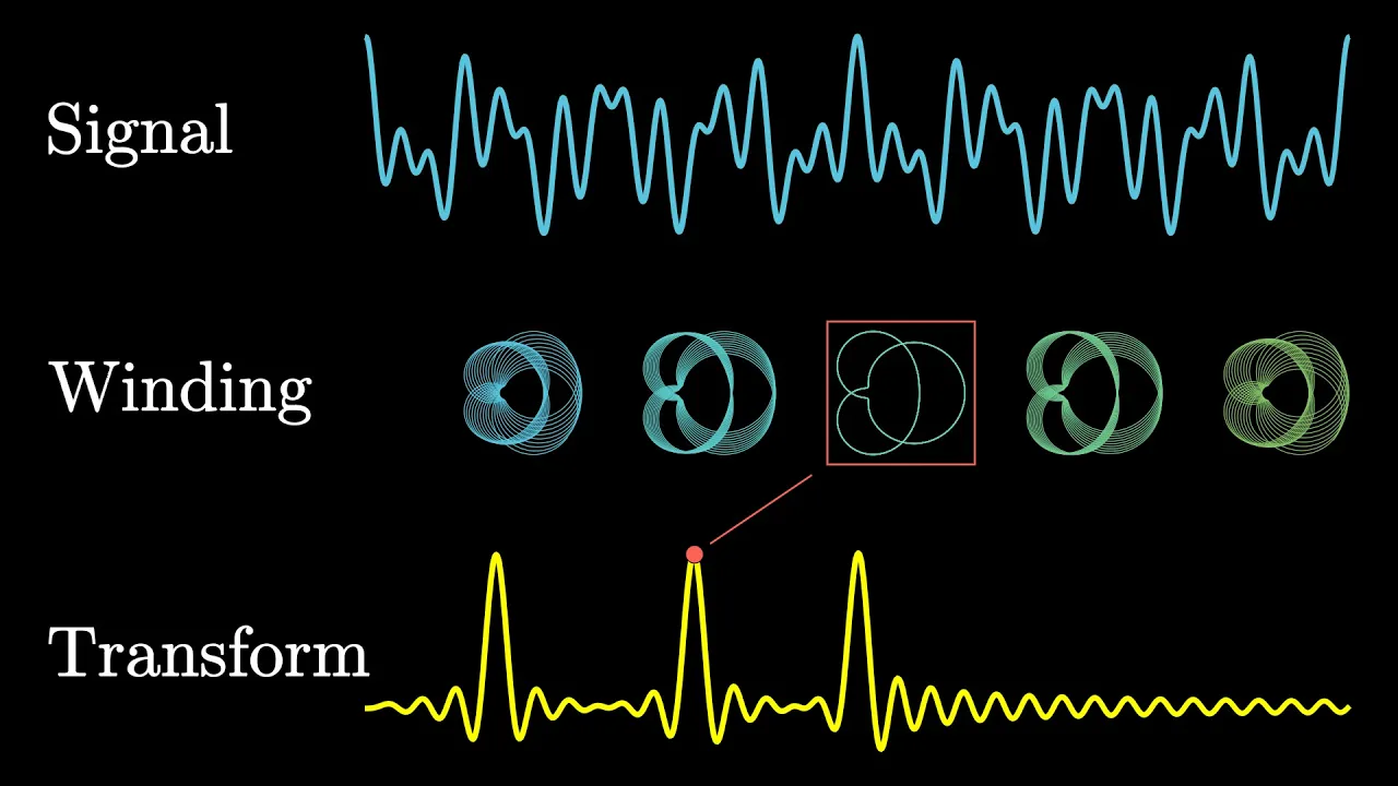
Wrapping a time-domain signal around a circle at variable rates isolates constituent frequencies because non-matching tones cancel out while resonant frequencies shift the curve's center of mass.
AI-assisted summary of But what is the Fourier Transform? A visual introduction. — original source. Check the original for full context.
Source published:
Key ideas
- The Fourier transform operates intuitively by wrapping a time-domain wave around a circle at varying winding rates and measuring the center of mass to detect resonant frequencies. (2:29)
- Because the winding operation is linear, combined audio waves decompose into sharp, isolated spikes corresponding directly to each constituent pure frequency. (8:07)
- The formal Fourier transform equation encapsulates circular winding using Euler's formula in the expression $g(t)e^{-2\pi i f t}$, omitting duration normalization so that sustained frequencies scale proportionally with signal length. (14:43)
- Beyond audio filtering, the Fourier transform maps functions of time into complex-valued functions of frequency that encode both amplitude and phase across physics and pure mathematics. (17:08)
Detailed notes
## Background Published by Grant Sanderson on the YouTube channel 3Blue1Brown on January 26, 2018, this video provides an animated visual introduction to the Fourier transform. The video description frames the lesson as an intuitive exploration of frequency decomposition, made largely using Sanderson's custom Python animation library, manim.
## TL;DR The video demystifies the Fourier transform by presenting an intuitive visual metaphor: taking a time-domain wave and wrapping it around a circle at varying winding frequencies using a rotating vector. When the winding rate aligns with a frequency component present in the signal, the wound-up curve bunches toward one side, causing its center of mass to spike away from the origin. Sanderson formalizes this geometric mechanism into Euler's formula and complex numbers, showing how the term e^(-2πi f t) naturally handles clockwise circular rotation. Finally, by transitioning from the average center of mass to an unnormalized integral over time, he constructs the complete mathematical definition of the Fourier transform, explaining how it cleanly extracts individual frequencies and phase information from blended signals.
## Atmosphere & style The presentation carries 3Blue1Brown's signature calm, elegant, and intellectually satisfying tone, backed by gentle ambient music from Vincent Rubinetti. Sanderson guides the viewer through complex calculus and abstract algebra with patient, grounded explanations, transforming what is often seen as an intimidating formula into an intuitive geometric machine. The visual progression feels smooth and mesmerizing as tangled, chaotic loops suddenly snap into clean, resonant alignments, instilling a genuine sense of aesthetic and conceptual clarity.
## Bulletin - [02:29](https://www.youtube.com/watch?v=spUNpyF58BY&t=149s) The Fourier transform operates intuitively by wrapping a time-domain wave around a circle at varying winding rates and measuring the center of mass to detect resonant frequencies. - [08:07](https://www.youtube.com/watch?v=spUNpyF58BY&t=487s) Because the winding operation is linear, combined audio waves decompose into sharp, isolated spikes corresponding directly to each constituent pure frequency. - [14:43](https://www.youtube.com/watch?v=spUNpyF58BY&t=883s) The formal Fourier transform equation encapsulates circular winding using Euler's formula in the expression $g(t)e^{-2\pi i f t}$, omitting duration normalization so that sustained frequencies scale proportionally with signal length. - [17:08](https://www.youtube.com/watch?v=spUNpyF58BY&t=1028s) Beyond audio filtering, the Fourier transform maps functions of time into complex-valued functions of frequency that encode both amplitude and phase across physics and pure mathematics.
## Key takeaways - [00:04](https://www.youtube.com/watch?v=spUNpyF58BY&t=4s) A recorded audio signal combines individual frequency oscillations into a single net air pressure graph over time, mixing constituent notes together. - [01:22](https://www.youtube.com/watch?v=spUNpyF58BY&t=82s) Decomposing an aggregated sound wave back into pure frequencies resembles unmixing distinct colors of stirred paint. - [02:29](https://www.youtube.com/watch?v=spUNpyF58BY&t=149s) The winding machine wraps a time-domain signal around the origin of a 2D plane by matching a rotating vector's magnitude to the signal's value at each moment. - [03:24](https://www.youtube.com/watch?v=spUNpyF58BY&t=204s) The geometric appearance of the wound-up graph is governed by the difference between the signal's intrinsic frequency and the chosen winding frequency. - [04:20](https://www.youtube.com/watch?v=spUNpyF58BY&t=260s) When the winding frequency matches the signal frequency, peaks align symmetrically on one side of the circle, pulling the center of mass away from the origin. - [04:59](https://www.youtube.com/watch?v=spUNpyF58BY&t=299s) Tracking the horizontal coordinate of the center of mass against winding frequency produces an 'almost Fourier transform' marked by sharp resonant peaks. - [08:07](https://www.youtube.com/watch?v=spUNpyF58BY&t=487s) Due to linearity, computing the transform of a sum of signals is identical to summing the transforms of each individual signal. - [09:34](https://www.youtube.com/watch?v=spUNpyF58BY&t=574s) Transform linearity allows complex, blended audio waves to be cleanly unmixed into distinct frequency spikes. - [10:55](https://www.youtube.com/watch?v=spUNpyF58BY&t=655s) Audio filtering isolates unwanted noise frequencies as distinct spikes in frequency space, allowing them to be suppressed before applying an inverse Fourier transform. - [11:49](https://www.youtube.com/watch?v=spUNpyF58BY&t=709s) The 2D plane is naturally formalized as the complex plane, where the center of mass is represented as a complex number with real and imaginary components. - [12:21](https://www.youtube.com/watch?v=spUNpyF58BY&t=741s) Euler's formula provides a compact mathematical notation, $e^{-2\pi i f t}$, to describe smooth, clockwise rotation at frequency $f$. - [13:52](https://www.youtube.com/watch?v=spUNpyF58BY&t=832s) Multiplying a signal $g(t)$ by $e^{-2\pi i f t}$ analytically models the physical process of winding the graph around a circle in the complex plane. - [14:43](https://www.youtube.com/watch?v=spUNpyF58BY&t=883s) The center of mass over a time window is formally computed as the continuous integral $\frac{1}{t_2 - t_1} \int_{t_1}^{t_2} g(t)e^{-2\pi i f t}\,dt$. - [15:32](https://www.youtube.com/watch?v=spUNpyF58BY&t=932s) The authentic Fourier transform drops the duration divisor $\frac{1}{t_2 - t_1}$, causing resonant peak magnitudes to scale linearly with how long a frequency persists. - [17:08](https://www.youtube.com/watch?v=spUNpyF58BY&t=1028s) The resulting Fourier transform $\hat{g}(f)$ maps frequency inputs to complex outputs whose magnitude represents frequency strength and whose angle represents phase. - [18:03](https://www.youtube.com/watch?v=spUNpyF58BY&t=1083s) Formal Fourier analysis evaluates limits spanning negative to positive infinity, underpinning advanced physics concepts including the Heisenberg uncertainty principle.
## Detailed walkthrough ### [00:04](https://www.youtube.com/watch?v=spUNpyF58BY&t=4s) Unmixing Sound: The Core Intuition of the Fourier Transform
The goal is to build an animated, visual understanding of one of the most vital concepts in mathematics: the Fourier transform. While the classical entry point is decomposing sound into constituent frequencies, the underlying idea stretches across wildly disparate fields of math and physics. As Grant Sanderson notes: “Really, it's crazy just how ubiquitous this idea is.”
To ground the concept, consider the sound of a pure concert A note at 440 beats (or cycles) per second. If you plot the air pressure next to a speaker or headphone as a function of time, it oscillates above and below its ambient equilibrium in a regular wave, completing 440 full oscillations every second. A lower note, such as a D, exhibits the exact same periodic wave shape, merely oscillating with fewer beats per second.
When two or more distinct notes are sounded simultaneously, the net pressure difference at any specific instant in time is simply the algebraic sum of the individual waves. At moments where the peaks align, the combined pressure surges; at other moments, a peak in one note encounters a trough in another, canceling out. As more notes are layered together, the combined pressure-versus-time graph rapidly becomes chaotic and irregular. Yet, despite how jagged and intricate the resulting wave appears, it contains only the underlying information of those few component frequencies. Because a physical microphone recording a performance registers only the total net air pressure at each moment, it captures only this aggregated sum. Decomposing that raw time-domain signal back into its pure, constituent frequencies presents a non-trivial challenge. Grant Sanderson summarizes the paradox: “Adding up those signals really mixes them all together, so pulling them back apart feels akin to unmixing multiple paint colors that have all been stirred up together.”
```mermaid flowchart TD accTitle: The Fourier Analysis Concept accDescr: Flowchart illustrating how mixed time-domain audio signals are decomposed into constituent frequencies using a winding machine.
subgraph TimeDomain["Time Domain (Combined Signal)"] A["Pure Note A (e.g., 440 Hz)"] --> C["Superposition: Mixed Waveform"] B["Pure Note D (Lower Pitch)"] --> C end
subgraph Machine["The Mathematical Machine"] C --> D["Wrap Wave Around Circle at Variable Winding Frequency"] D --> E["Calculate Center of Mass (x-coordinate)"] end
subgraph FrequencyDomain["Frequency Domain (Decomposition)"] E --> F["Fourier Peak at Note D Frequency"] E --> G["Fourier Peak at Note A Frequency"] end ```
[02:29](https://www.youtube.com/watch?v=spUNpyF58BY&t=149s) The Winding Machine: Wrapping Graphs Around a Circle
To separate the blended frequencies, the strategy is to design a mathematical mechanism that treats a specific target frequency fundamentally differently from all others. To trace the mechanics cleanly, start with a simple, pure test signal oscillating at a manageable rate of just 3 beats per second, plotted over a finite interval from $t = 0$ seconds to $t = 4.5$ seconds. The central conceptual trick is to take this linear wave graph and literally wrap it around a circle.
Concretely, this wrapping process is carried out by an imaginary rotating vector originating from the center of a two-dimensional plane. At every moment in time, the length of the vector equals the height of the signal graph at that precise timestamp. High points on the waveform cause the vector to extend far from the origin, while valleys keep it pulled in close. Simultaneously, the vector rotates around the origin at a chosen winding rate. For instance, if traversing 2 seconds of time along the original wave corresponds to completing one full $360^\circ$ circle, the vector rotates at a winding frequency of half a cycle per second ($0.5\text{ Hz}$).
Crucially, this setup involves two entirely distinct frequencies: - The intrinsic frequency of the signal itself (here, oscillating 3 times per second). - The winding frequency at which the graph is being wrapped around the origin.
Adjusting this winding frequency alters the visual geometry of the wound-up graph, producing shapes ranging from lopsided spirals to intricate circular petals. Grant Sanderson emphasizes: “And that choice of winding frequency determines what the wound up graph looks like.” To track these relationships visually, vertical reference markers spaced across the linear wave indicate intervals corresponding to one full revolution around the circle (for instance, markers spaced every 1.5 seconds when the winding period is 1.5 seconds). When the winding frequency is dialed until it matches the internal frequency of the wave (3 cycles per second), something dramatic happens: all the peaks of the wave line up on the right-hand side of the circle, while all the valleys concentrate on the left.
[04:59](https://www.youtube.com/watch?v=spUNpyF58BY&t=299s) Finding the Center of Mass and the "Almost Fourier Transform"
To turn this geometric alignment into a concrete metric, imagine the wound-up graph as a physical wire having uniform mass. Because mass tracks the wire's length, the center of mass of this wire provides an exact summary of where the curve concentrates in the plane. For the vast majority of winding frequencies, the peaks and troughs distribute fairly evenly around the circumference, meaning their pull balances out and the center of mass hovers very close to the central origin.
However, when the winding frequency matches the signal frequency (3 beats per second), the wire's long extensions consistently align toward the right, pulling the center of mass unusually far in that positive direction. Tracking only the horizontal ($x$) coordinate of this center of mass as a function of the winding frequency yields a new graph: - Near a winding frequency of 0, everything bunches up on the positive side because the original wave was shifted upward into strictly positive values, creating a large initial spike at zero. - As the winding frequency increases, the peaks distribute around the circle, dropping the center of mass toward zero, where it gently wobbles. - At exactly 3 cycles per second, the center of mass surges outward, creating a distinct, sharp peak on the plot.
Grant Sanderson describes this resulting plot: “This whole plot is what I'll call the almost Fourier transform of the original signal.” He clarifies that while the spike at zero is merely an artifact of shifting the wave upward above the horizontal axis to keep values intuitive, the defining feature of interest for decomposing frequencies is that resonant bump at 3. Running the same process on a pure 2-beat-per-second wave produces an identical characteristic spike centered cleanly at 2 cycles per second.
- The center of mass is fundamentally a two-dimensional coordinate $(x, y)$, but tracking just the horizontal $x$-coordinate is sufficient to demonstrate the resonance effect. - A signal oscillating symmetrically around zero (with negative values) eliminates the artificial zero-frequency spike, leaving only the resonant peak at the true frequency.
[08:07](https://www.youtube.com/watch?v=spUNpyF58BY&t=487s) Linearity and Unmixing Multiple Frequencies
The true power of this winding mechanism emerges when processing a combined wave made by adding a 2-cycle-per-second wave and a 3-cycle-per-second wave together. The combined wave looks noticeably distorted and lacks the clean simplicity of a single cosine curve. When wrapped around the circle, it generally appears as a tangled, chaotic nest of loops. Yet, as the winding dial sweeps through frequencies, the chaos momentarily crystallizes into an aligned loop at 2 cycles per second, drops back into disorder, and then aligns again at 3 cycles per second.
This occurs because of linearity: computing the center-of-mass winding transform on individual signals and adding those outputs together yields the exact same curve as adding the signals first and then running the transform. Grant Sanderson highlights the utility of this mathematical property: “Now this property makes things really useful to us, because the transform of a pure frequency is close to zero everywhere except for a spike around that frequency, so when you add together two pure frequencies, the transform graph just has these little peaks above the frequencies that went into it.”
Because the winding transform produces near-zero values across non-matching frequencies and produces distinct spikes only at resonant frequencies, the transform of an aggregated wave simply displays clean, isolated peaks matching each individual component. The machine successfully unmixes the blended signal, separating out the original ingredients just as one might hope to separate mixed paints. This operation serves immediate practical applications, such as audio editing, where an unwanted high-pitched drone in a time-domain recording can be isolated in the frequency spectrum and cleanly filtered out.
[10:55](https://www.youtube.com/watch?v=spUNpyF58BY&t=655s) Filtering Frequencies and the Complex Plane
Viewing an audio signal purely as raw voltage supplied to a speaker millisecond by millisecond obscures its harmonic structure. When that signal is converted into frequency space via the Fourier transform, an annoying high-pitched noise ceases to be an intractable mess in time and instead isolates cleanly into an individual spike at a high frequency. Removing that nuisance is conceptually as simple as smushing down that unwanted spike. The resulting modified plot represents the Fourier transform of the clean audio, and an operation known as the inverse Fourier transform reconstructs the exact time-domain sound wave corresponding to that filtered profile. As Grant Sanderson notes when introducing this duality, “applying the Fourier transform to the Fourier transform gives you back something close to the original function.”
```mermaid flowchart LR accTitle: Audio Filtering with the Fourier Transform accDescr: Pipeline showing sound transformed to frequency space, filtered, and inverted back to audio. subgraph TimeDomain1["Time Domain"] A["Original Audio Signal<br/>(voltage vs. time)"] end subgraph FrequencyDomain["Frequency Domain"] B["Fourier Transform<br/>(frequency spectrum)"] C["Filtered Spectrum<br/>(smush high-pitch spike)"] end subgraph TimeDomain2["Clean Time Domain"] D["Inverse Fourier Transform<br/>(cleaned sound wave)"] end
A -->|"Fourier transform"| B B -->|"Filter noise"| C C -->|"Inverse transform"| D ```
Calling repeated Fourier transformation the exact path back to the original function is an instructive slight oversimplification, largely because tracking only the horizontal center of mass of the wound-up graph ignores critical geometry. A two-dimensional wound-up plot possesses both an $x$-coordinate and a $y$-coordinate. Rather than treating these coordinates as disconnected pairs of real numbers, mathematical convention packages them into the complex plane, where the center of mass is a single complex number composed of a real part and an imaginary part.
- Audio filtering operates by identifying specific frequency spikes, attenuating or zeroing them out, and synthesizing the remaining components back into the time domain. - The two-dimensional coordinates of the wound-up path map naturally to complex numbers of the form $x + iy$. - Complex numbers provide the natural mathematical language for describing circular motion, winding, and phase.
---
[12:21](https://www.youtube.com/watch?v=spUNpyF58BY&t=741s) Euler’s Formula and the Winding Expression
Complex numbers excel at modeling winding and circular rotation because of Euler's formula. When evaluating $e$ raised to an imaginary power, $e^{i\theta}$, the resulting value lands on the point located $\theta$ units counterclockwise along the unit circle starting from $(1, 0)$ on the positive real axis. A full revolution requires tracing the circle's circumference of $2\pi$, so a rotation at a standard rate of 1 cycle per second is written as $e^{2\pi i t}$, where $t$ denotes elapsed time. To adjust this pace to any desired frequency $f$, time is multiplied by $f$ in the exponent, yielding $e^{2\pi i f t}$. For instance, setting $f = \frac{1}{10}$ forces $t$ to advance all the way to 10 seconds before the exponent reaches $2\pi i$, thereby completing one gentle rotation every 10 seconds.
In Fourier analysis, the standard convention is to rotate clockwise rather than counterclockwise, requiring a negative sign inside the exponent. If a time-varying intensity signal $g(t)$ multiplies this rotating exponential, the unit-length rotating vector scales up and down according to the instantaneous amplitude of $g(t)$. The tip of this changing vector sketches out the wound-up signal in the complex plane across time. Sanderson marvels at the compactness of this description: “So think about it, this is awesome, this really small expression is a super elegant way to encapsulate the whole idea of winding a graph around a circle with a variable frequency, $f$.”
- Euler's formula establishes that $e^{i\theta} = \cos(\theta) + i\sin(\theta)$, placing values on a unit circle centered at the origin. - The term $e^{-2\pi i f t}$ governs clockwise rotation at a frequency of $f$ cycles per unit time. - Multiplying $g(t) \cdot e^{-2\pi i f t}$ scales the rotating complex exponential by the signal's value at time $t$, exactly implementing the winding machine.
---
[14:43](https://www.youtube.com/watch?v=spUNpyF58BY&t=883s) From Center of Mass to the Actual Fourier Transform
To compute the center of mass of this wound-up curve mathematically, one can sample points at regular time intervals, sum their complex positions, and divide by the total sample count. Taking the limit as the sample points become infinitely dense replaces the discrete arithmetic average with an integral divided by the total duration: $\frac{1}{t_2 - t_1} \int_{t_1}^{t_2} g(t)e^{-2\pi i f t}\,dt$. While integrating a complex-valued function can appear intimidating to students rusty with calculus, its geometric meaning is completely unpretentious: it merely identifies the balance point of the wound curve in the complex plane.
```mermaid flowchart TD accTitle: Construction of the Fourier Transform Formula accDescr: Progression from discrete sampling to the continuous center of mass, and finally to the unnormalized Fourier integral. A["Sample Discrete Complex Points<br/>g(t) · e^(-2πi f t)"] --> B["Compute Sample Average<br/>(Sum of points / N)"] B --> C["Continuous Center of Mass<br/>(1 / Δt) ∫ g(t) e^(-2πi f t) dt"] C -->|"Drop the (1 / Δt) scale factor"| D["Honest Fourier Transform<br/>G(f) = ∫ g(t) e^(-2πi f t) dt"] ```
The transition from this physical center of mass to the actual, honest-to-goodness Fourier transform involves one crucial modification: dropping the division by the time interval length. The true Fourier transform is strictly the integral part, $\int g(t)e^{-2\pi i f t}\,dt$. Omitting the time divisor means the output scales proportionally with the duration over which a frequency persists. If a pure 2-beat-per-second signal is wound at 2 cycles per second, its center of mass remains anchored at the same offset point whether the clip lasts 3 seconds or 6 seconds; however, its Fourier transform magnitude doubles from a factor of 3 to a factor of 6. Meanwhile, non-matching frequencies loop evenly around the origin, experiencing near-complete cancellation as longer observation windows give the graph more opportunities to balance out.
- The center of mass of a continuous wound-up curve over an interval is $\frac{1}{t_2 - t_1} \int_{t_1}^{t_2} g(t)e^{-2\pi i f t}\,dt$. - The authentic Fourier transform omits the normalization factor $\frac{1}{t_2 - t_1}$. - Scaling with signal length ensures that sustained frequencies accumulate greater transform magnitudes, cleanly separating persistent pure tones from transient noise.
---
[17:08](https://www.youtube.com/watch?v=spUNpyF58BY&t=1028s) The Fourier Transform Function and Infinite Limits
Synthesizing all these moving parts reveals the structural definition of the transform. The Fourier transform maps a function of time, $g(t)$, into a brand-new function of frequency, universally denoted as $\hat{g}(f)$ (spoken as "$g$-hat"). The output of $\hat{g}(f)$ is a complex number whose distance from the origin encodes the strength of frequency $f$ within the original signal, while its angular orientation encodes the phase. Graphs depicting the transform often plot the real component (the horizontal balance coordinate), though graphing the imaginary component provides equal mathematical fidelity.
Although real-world audio engineering and data processing inherently operate across finite recording durations, formal mathematical theory defines the transform over the infinite horizon: $$\hat{g}(f) = \int_{-\infty}^{\infty} g(t)e^{-2\pi i f t}\,dt$$ This represents the limit of the integral evaluated across finite windows as the bounds expand toward negative and positive infinity. Reflecting on the synthesis, Sanderson emphasizes: “And out of context, you can imagine how seeing this formula would seem sort of daunting, but if you understand how exponentials correspond to rotation, how multiplying that by the function $g(t)$ means drawing a wound up version of the graph, and how an integral of a complex valued function can be interpreted in terms of a center of mass idea, you can see how this whole thing carries with it a very rich intuitive meaning.” He concludes by previewing that the Fourier transform reaches into far deeper areas of mathematics and physics—including the Heisenberg uncertainty principle—well beyond simple frequency extraction from audio signals.
- Input to $\hat{g}$: frequency $f$ (winding frequency). Output of $\hat{g}$: a complex number capturing amplitude and phase. - Practical signal analysis integrates over bounded windows $[t_1, t_2]$, whereas formal theory evaluates limits spanning $-\infty$ to $\infty$. - The machinery serves as the bedrock for wave mechanics, partial differential equations, and quantum uncertainty.
## Notable quotes > [10:55](https://www.youtube.com/watch?v=spUNpyF58BY&t=655s) applying the Fourier transform to the Fourier transform gives you back something close to the original function. — Grant Sanderson
## Mentioned 3Blue1Brown, Grant Sanderson, Leonhard Euler, Werner Heisenberg, Vincent Rubinetti, Jane Street, Manim, Prajwal Souza, Omer Tuchfeld
## Video description An animated introduction to the Fourier Transform. Help fund future projects: https://www.patreon.com/3blue1brown An equally valuable form of support is to simply share some of the videos. Special thanks to these supporters: http://3b1b.co/fourier-thanks Learn more about Janestreet: https://janestreet.com/3b1b
Follow-on video about the uncertainty principle: https://youtu.be/MBnnXbOM5S4
Interactive made by a viewer inspired by this video: https://prajwalsouza.github.io/Experiments/Fourier-Transform-Visualization.html
Also, take a look at this Jupyter notebook implementing this idea in a way you can play with: https://github.com/thatSaneKid/fourier/blob/master/Fourier%20Transform%20-%20A%20Visual%20Introduction.ipynb
Thanks to these viewers for their contributions to translations Hebrew: Omer Tuchfeld Russian: xX-Masik-Xx Vietnamese: @ngvutuan2811
------------------ Animations largely made using manim, a scrappy open-source python library. https://github.com/3b1b/manim
If you want to check it out, I feel compelled to warn you that it's not the most well-documented tool, and has many other quirks you might expect in a library someone wrote with only their own use in mind.
Music by Vincent Rubinetti. Download the music on Bandcamp: https://vincerubinetti.bandcamp.com/album/the-music-of-3blue1brown
Stream the music on Spotify: https://open.spotify.com/album/1dVyjwS8FBqXhRunaG5W5u
If you want to contribute translated subtitles or to help review those that have already been made by others and need approval, you can click the gear icon in the video and go to subtitles/cc, then "add subtitles/cc". I really appreciate those who do this, as it helps make the lessons accessible to more people. ------------------
3blue1brown is a channel about animating math, in all senses of the word animate. And you know the drill with YouTube, if you want to stay posted on new videos, subscribe, and click the bell to receive notifications (if you're into that).
If you are new to this channel and want to see more, a good place to start is this playlist: http://3b1b.co/recommended
Various social media stuffs: Website: https://www.3blue1brown.com Twitter: https://twitter.com/3Blue1Brown Patreon: https://patreon.com/3blue1brown Facebook: https://www.facebook.com/3blue1brown Reddit: https://www.reddit.com/r/3Blue1Brown
[Source](https://www.youtube.com/watch?v=spUNpyF58BY)