3Blue1Brown Strips Neural Nets to 13,000 Matrix-Vector Operations
3Blue1Brown
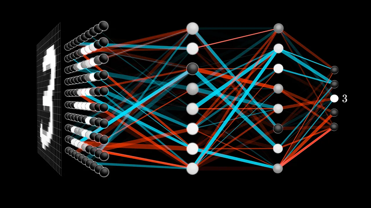
Layered neural networks resolve complex recognition tasks not through biological mimicry, but by chaining 13,000 tunable linear algebra parameters that assemble raw pixels into hierarchical geometric features.
AI-assisted summary of But what is a neural network? | Deep learning chapter 1 — original source. Check the original for full context.
Source published:
Key ideas
- A plain vanilla neural network maps high-dimensional inputs directly to category predictions, exemplified by a 4-layer network that transforms 784 grayscale pixels into 10 digit probabilities via roughly 13,000 tunable parameters. (10:38)
- The computational structure relies on hierarchical abstraction, where initial layers detect localized edges, intermediate layers combine edges into components, and final layers classify complete patterns. (5:31)
- Layer-to-layer forward propagation is compactly vectorized as σ(Wa + b), turning the entire network into a single deterministic mathematical function mapping ℝ⁷⁸⁴ to ℝ¹⁰. (13:26)
- While historically grounded in the sigmoid activation function σ(x) = 1 / (1 + e⁻ˣ), modern deep learning predominantly uses ReLU, max(0, a), due to severe training difficulties encountered with deep sigmoidal networks. (17:03)
Detailed notes
## Background This video was published on YouTube by 3Blue1Brown on October 5, 2017, as the opening chapter of a deep learning series. According to the description, the video explores what artificial neurons are, why neural networks are structured in sequential layers, and the core mathematical framework underpinning their operation.
## TL;DR Using the classic problem of handwritten digit recognition on a 28×28 pixel grid as a motivating example, the video strips away machine learning buzzwords to explain the plain-vanilla multilayer perceptron. It defines a neuron as a container for an activation value and demonstrates how stacking layers enables hierarchical feature abstraction, from localized edges to composite shapes. The lesson details the mechanics of computing weighted sums and biases across nearly 13,000 parameters, expresses layer transitions cleanly via matrix-vector multiplication as $\sigma(Wa + b)$, and concludes with a discussion alongside guest researcher Lisha Li on why modern deep learning architectures often favor ReLU over the traditional sigmoid function.
## Atmosphere & style The presentation carries 3Blue1Brown's signature calm, elegant, and intellectually reassuring tone, grounding complex concepts in lucid geometric intuitions and smooth custom animations. Grant Sanderson speaks with measured curiosity and warmth, demystifying intimidating mathematical notation into approachable, tactile analogies like turning 13,000 dials. The brief, collaborative closing segment with guest Lisha Li adds an engaging, real-world research perspective, leaving the viewer feeling quietly empowered rather than overwhelmed by mathematical abstraction.
## Bulletin - [10:38](https://www.youtube.com/watch?v=aircAruvnKk&t=638s) A plain vanilla neural network maps high-dimensional inputs directly to category predictions, exemplified by a 4-layer network that transforms 784 grayscale pixels into 10 digit probabilities via roughly 13,000 tunable parameters. - [05:31](https://www.youtube.com/watch?v=aircAruvnKk&t=331s) The computational structure relies on hierarchical abstraction, where initial layers detect localized edges, intermediate layers combine edges into components, and final layers classify complete patterns. - [13:26](https://www.youtube.com/watch?v=aircAruvnKk&t=806s) Layer-to-layer forward propagation is compactly vectorized as σ(Wa + b), turning the entire network into a single deterministic mathematical function mapping ℝ⁷⁸⁴ to ℝ¹⁰. - [17:03](https://www.youtube.com/watch?v=aircAruvnKk&t=1023s) While historically grounded in the sigmoid activation function σ(x) = 1 / (1 + e⁻ˣ), modern deep learning predominantly uses ReLU, max(0, a), due to severe training difficulties encountered with deep sigmoidal networks.
## Key takeaways - [00:04](https://www.youtube.com/watch?v=aircAruvnKk&t=4s) Algorithmic digit recognition on raw 28x28 pixel grids is exceptionally difficult for conventional rule-based code, prompting the use of data-driven neural networks. - [01:07](https://www.youtube.com/watch?v=aircAruvnKk&t=67s) The focus of the exploration is on the foundational 'plain vanilla' multilayer perceptron structure before examining how optimization and learning occur. - [02:42](https://www.youtube.com/watch?v=aircAruvnKk&t=162s) An artificial neuron is fundamentally a container holding an activation value bounded between 0.0 and 1.0. - [03:35](https://www.youtube.com/watch?v=aircAruvnKk&t=215s) The demonstrated architecture consists of 784 input neurons, two hidden layers of 16 neurons each, and 10 output neurons representing digits 0 through 9. - [05:31](https://www.youtube.com/watch?v=aircAruvnKk&t=331s) Layered architectures leverage hierarchical abstraction to break complex visual recognition tasks into lower-level edge and component detection problems. - [07:30](https://www.youtube.com/watch?v=aircAruvnKk&t=450s) Hierarchical decomposition applies beyond visual cognition to domains like speech recognition, which chains audio waveforms into phonemes, syllables, words, and phrases. - [08:38](https://www.youtube.com/watch?v=aircAruvnKk&t=518s) Weights determine what specific spatial pattern of pixels or previous-layer activations a neuron responds to, using positive, negative, or near-zero values. - [09:45](https://www.youtube.com/watch?v=aircAruvnKk&t=585s) The sigmoid function squashes arbitrary real-valued weighted sums into a smooth output interval between 0 and 1. - [10:38](https://www.youtube.com/watch?v=aircAruvnKk&t=638s) Biases act as activation thresholds, dictating how large the incoming weighted sum must be before a neuron becomes meaningfully active. - [11:34](https://www.youtube.com/watch?v=aircAruvnKk&t=694s) The 784-16-16-10 architecture contains almost exactly 13,000 weights and biases, which serve as the adjustable knobs tuned during the learning process. - [12:30](https://www.youtube.com/watch?v=aircAruvnKk&t=750s) Understanding the functional role of weights and biases prevents practitioners from treating neural networks purely as opaque black boxes. - [13:26](https://www.youtube.com/watch?v=aircAruvnKk&t=806s) Linear algebra condenses network computations into the matrix-vector form σ(Wa + b), drastically speeding up execution in modern numerical software. - [15:10](https://www.youtube.com/watch?v=aircAruvnKk&t=910s) The entire neural network functions as a single high-dimensional mathematical function mapping 784 real inputs to 10 output values. - [17:03](https://www.youtube.com/watch?v=aircAruvnKk&t=1023s) Modern architectures favor the Rectified Linear Unit (ReLU), defined as max(0, a), because it trains far more effectively in deep networks than traditional sigmoids.
## Detailed walkthrough ### [00:04](https://www.youtube.com/watch?v=aircAruvnKk&t=4s) The Challenge of Recognizing Handwritten Digits
Visual recognition appears completely effortless to the human brain, but it is computationally staggering. A handwritten numeral "3", scrawled sloppily and rendered onto an extremely coarse grid of just 28 by 28 pixels, is identified by the human eye without hesitation. Even when presented with multiple variations of the digit—each possessing radically different individual pixel values and triggering entirely different photoreceptors in the eye—the visual cortex seamlessly interprets them as representing the exact same conceptual numeral, while simultaneously categorizing other configurations as distinct numbers altogether.
```mermaid flowchart LR accTitle: MNIST Digit Classification Pipeline accDescr: An input 28x28 image flows into a network of 784 inputs, two hidden layers, and ten outputs. subgraph IN["Input Stage"] IMG["28x28 Image"] --> L1["Layer 1: 784 Neurons"] end subgraph HID["Hidden Processing"] L1 --> L2["Layer 2: 16 Neurons"] L2 --> L3["Layer 3: 16 Neurons"] end subgraph OUT["Output Stage"] L3 --> L4["Layer 4: 10 Neurons<br/>(Digits 0–9)"] end ```
The difficulty becomes obvious the moment one attempts to formalize this process algorithmically. As Grant Sanderson observes: “But if I told you, hey, sit down and write for me a program that takes in a grid of 28x28 pixels like this and outputs a single number between 0 and 10, telling you what it thinks the digit is, well the task goes from comically trivial to dauntingly difficult.” Modern machine learning tackles this very gap by abandoning rigid rule-writing in favor of mathematical structures that learn directly from data.
- Input image size: 28 × 28 grayscale pixels (784 total values) - Program objective: Map the raw pixel array to an integer prediction from 0 to 9
---
[01:07](https://www.youtube.com/watch?v=aircAruvnKk&t=67s) Demystifying Neural Networks: Vanilla Architecture Over Hype
While machine learning and artificial intelligence are saturated with industry buzzwords, the core objective here is to demystify what a neural network actually represents from a purely mathematical standpoint, assuming zero prior background. Rather than tackling complex, modern architectural variations that have exploded throughout recent research, this exploration focuses on the foundational, "plain vanilla" multilayer perceptron without extra frills.
This introductory setup splits the conceptual framework into two distinct halves: first, understanding the physical and mathematical anatomy of the network structure itself, and second, understanding what it actually means when a network undergoes the process of "learning." Even in its most basic, unadorned state, a simple neural network possesses enough expressive power to classify handwritten digits, while simultaneously exhibiting clear, instructive limitations in how it handles visual data.
---
[02:42](https://www.youtube.com/watch?v=aircAruvnKk&t=162s) Deconstructing the Neuron and Network Layers
Stripping away biological romanticism, an artificial neuron is fundamentally just a container holding a real number—specifically, an "activation" value bounded between 0 and 1. The full network is organized into sequential layers of these containers:
```mermaid flowchart TD accTitle: Forward Layer Propagation accDescr: Propagation from input pixels through hidden feature detectors to final output digits. subgraph L_IN["Input Layer"] P["784 Neurons<br/>(Pixel Brightness: 0.0 to 1.0)"] end subgraph L_HID["Hidden Layers"] H1["Hidden Layer 1<br/>(16 Neurons: Edge Detectors)"] H2["Hidden Layer 2<br/>(16 Neurons: Pattern Assemblers)"] end subgraph L_OUT["Output Layer"] O["10 Neurons<br/>(Digit Confidences: 0 to 9)"] end P -->|"Weighted Influence"| H1 H1 -->|"Weighted Influence"| H2 H2 -->|"Weighted Influence"| O ```
The first layer contains 784 neurons, corresponding to every single pixel in the 28×28 input image. The activation of each input neuron mirrors the grayscale intensity of its assigned pixel, scaling from 0 for pure black up to 1 for pure white. At the opposite end stands the output layer, made up of 10 neurons corresponding to the digits 0 through 9; here, an activation near 1 signals high confidence from the model that the input matches that digit.
Between input and output sit two "hidden layers," each arbitrarily chosen to contain 16 neurons. As Sanderson points out regarding this concrete design choice: “To be honest I chose two layers based on how I want to motivate the structure in just a moment, and 16, well that was just a nice number to fit on the screen.” When an image is fed forward through the network, the activation pattern of the input layer triggers a cascade of activity through the hidden layers, culminating in an output layer where the neuron glowing with the highest activation represents the network's final classification decision.
- Input layer dimension: 784 neurons ($28 \times 28$) - Hidden layers: 2 intermediate layers containing 16 neurons each - Output layer dimension: 10 neurons (representing classifications 0 through 9) - Neuron activation limits: Real numbers restricted between 0.0 (completely off) and 1.0 (fully lit)
---
[05:31](https://www.youtube.com/watch?v=aircAruvnKk&t=331s) Why Layers? Hierarchies of Abstraction
The intuitive justification for stacking neurons into successive layers is the concept of hierarchical abstraction. Human visual cognition naturally deconstructs complex geometries into constituent subcomponents: a digit "9" consists of an upper loop connected to a vertical right-hand stroke; an "8" is composed of two vertically stacked loops; and a "4" is an assembly of three distinct straight lines.
```mermaid flowchart TD accTitle: Hierarchical Feature Composition accDescr: How raw pixels aggregate into edges, components, and finally complete digit classifications. E["Layer 2: Local Edges & Slits"] --> C["Layer 3: Subcomponents<br/>(e.g., Upper Loops, Long Lines)"] C --> D["Layer 4: Full Digits<br/>(e.g., 8, 9, 4)"] ```
In an ideal system, one would hope that neurons in the penultimate layer fire whenever generalized, high-level features appear—such as detecting an upper loop regardless of its exact pixel alignment. That detection task itself naturally breaks down into an even lower tier of sub-problems: recognizing the individual directional edges that form the boundaries of that loop. Sanderson notes that this hierarchical principle extends far beyond vision: “And even beyond image recognition, there are all sorts of intelligent things you might want to do that break down into layers of abstraction.” Speech recognition systems operate under the exact same paradigm, assembling raw sound waves into phonemes, syllables, words, and eventually high-level sentences.
---
[08:38](https://www.youtube.com/watch?v=aircAruvnKk&t=518s) Edge Detection and the Math of Weighted Sums
To translate this conceptual hierarchy into functional mathematics, every neuron in a given layer is connected to every neuron in the preceding layer, with each connection governed by an adjustable real number called a **weight**. To determine the activation of a target neuron in the second layer—such as one intended to detect an edge in a localized region—the network computes a weighted sum of all incoming activations from the first layer.
```mermaid flowchart LR accTitle: Neuron Weighted Sum and Activation accDescr: Inputs are multiplied by weights, summed together, and passed through a sigmoid function. subgraph Inputs["Previous Layer Activations"] A1["a₁"] A2["a₂"] AN["aₙ"] end subgraph Computation["Target Neuron"] SUM["Weighted Sum:<br/>∑ (wᵢ · aᵢ)"] SIG["Sigmoid Squishing:<br/>σ(x) = 1 / (1 + e⁻ˣ)"] end A1 -->|"w₁"| SUM A2 -->|"w₂"| SUM AN -->|"wₙ"| SUM SUM --> SIG SIG --> OUT["Activation (0 to 1)"] ```
Visually, these weights can be organized into a spatial grid mapping directly onto the input image's geometry: - **Positive weights (green):** Pixels in the desired edge region are assigned positive weights, meaning bright pixels in this specific area increase the sum. - **Negative weights (red):** Pixels in the immediate surrounding periphery are assigned negative weights, penalizing activations if light spills outside the target boundary. - **Zero weights:** Irrelevant background pixels across the rest of the image receive weights near zero, nullifying their impact on the computation.
Because summing these raw products can yield arbitrary real numbers far outside the unit interval, the total weighted sum must be squashed back down into a valid activation value between 0 and 1. This normalization is achieved by passing the raw sum through an activation function, historically the **sigmoid function** (also known as the logistic curve):
$$\sigma(x) = \frac{1}{1 + e^{-x}}$$
This mathematical step ensures that regardless of how large or negative the linear combination of inputs becomes, the resulting activation remains smoothly bounded within the expected $[0, 1]$ operational range.
[10:38](https://www.youtube.com/watch?v=aircAruvnKk&t=638s) Biases, Parameter Counts, and the 13,000 Knobs and Dials
When a weighted sum of inputs passes into the sigmoid squishification function, very negative inputs get mapped close to 0, positive inputs get mapped close to 1, and the curve climbs steadily around an input of 0. In this setup, a neuron's activation is essentially an indicator of how positive its weighted sum happens to be. However, you might not want a neuron to fire just because its weighted sum barely creeps above zero. You might prefer that it only turns on if the weighted sum crosses a higher threshold—say, greater than 10. To introduce a preference or bias toward inactivity, you simply add an offset such as -10 to the weighted sum before passing the total through the sigmoid squishification function. This extra offset is formally called the bias. In intuitive terms, the weights govern what specific spatial pattern of pixels or earlier activations a neuron responds to, while the bias determines how high that weighted sum must climb before the neuron becomes meaningfully active.
Scaling this logic up across the entire architecture reveals just how vast the parameter space truly is. A single neuron in the second layer connects to all 784 pixel neurons from the first layer, demanding 784 individual weights alongside its own bias. With 16 neurons in that first hidden layer, connecting layer one to layer two requires 784 times 16 weights plus 16 biases. Factoring in the connections flowing into the next hidden layer and finally out to the ten output digits, the entire network contains almost exactly 13,000 total weights and biases. When machine learning researchers talk about “learning,” they are describing the algorithmic process of nudging and turning these 13,000 individual knobs and dials until the network settles on a configuration that solves the task.
Pondering that complexity leads to a thought experiment that is equal parts entertaining and daunting: sitting down and manually setting every single one of those 13,000 numbers by hand, deliberately adjusting parameters so that the second layer captures edges and the third layer detects composite loops. While modern practitioners rely on automated optimization, Grant Sanderson emphasizes the value of understanding the underlying mechanics rather than treating the model as an opaque black box: “I personally find this satisfying rather than just treating the network as a total black box, because when the network doesn't perform the way you anticipate, if you've built up a little bit of a relationship with what those weights and biases actually mean, you have a starting place for experimenting with how to change the structure to improve.”
```mermaid flowchart LR accTitle: Single Neuron Activation Flow accDescr: Diagram showing inputs multiplied by weights, summed with a bias, and passed through a sigmoid function. subgraph Inputs["Previous Layer"] A["Activations a₀, a₁,... aₙ"] end subgraph Processing["Neuron Computation"] B["Weighted Sum: Σ(wᵢ · aᵢ)"] C["Add Bias: + b"] D["Sigmoid Squishification: σ(...)"] end subgraph Output["Current Layer"] E["Activation a'"] end A --> B B --> C C --> D D --> E ```
- Each weight indicates what pattern of pixels or previous-layer features a neuron looks for. - Each bias sets the activation threshold, determining how positive the weighted sum must be to ignite the neuron. - Layer 1 (784 neurons) to Layer 2 (16 neurons) uses 12,544 weights ($784 \times 16$) plus 16 biases. - The full demo network spans four layers ($784 \to 16 \to 16 \to 10$) totaling almost exactly 13,000 tunable parameters.
---
[13:26](https://www.youtube.com/watch?v=aircAruvnKk&t=806s) Compact Matrix Notation and the Network as a Function
Writing out weighted sums and biases across thousands of individual connections quickly becomes cumbersome, which is why neural network operations are universally expressed using linear algebra. All activations from an incoming layer are collected into a vertical column vector, while the weights linking that layer to the next are organized into a matrix where each row corresponds to all incoming connections feeding into a single destination neuron. Multiplying this weight matrix by the activation vector produces a new vector containing the raw weighted sums for every destination neuron in one fell swoop. The biases are grouped into their own vector and added directly to that product. Finally, applying the sigmoid function across the outside simply squishes each individual component of the resulting vector into a value between 0 and 1.
Beyond making theoretical notation concise, grouping operations into $\sigma(Wa + b)$ provides massive computational advantages because modern numerical libraries are heavily optimized to execute matrix-vector multiplications at high speed. From this bird's-eye perspective, the earlier idea that neurons are mere containers for static numbers gives way to a more dynamic view: each neuron is fundamentally a mathematical function that digests activations from the previous layer and outputs a value between 0 and 1. By extension, the full network is nothing more than a giant, composite mathematical function that takes 784 numbers as input and outputs 10 numbers, parameterized by 13,000 weights and biases. Grant Sanderson notes that this staggering mathematical complexity should actually be comforting: “I mean if it were any simpler, what hope would we have that it could take on the challenge of recognizing digits?”
Closing out the mathematical walkthrough, Sanderson teases that the following video will demonstrate how networks actually learn these optimal weights and biases purely from training data. He also jokes about YouTube's notification bells, quipping that viewers should subscribe less for notifications and more to train YouTube's recommendation neural networks into realizing they want to see his videos. He thanks his Patreon supporters for their patience, noting that progress on his probability series slowed down over the summer but will resume immediately after finishing this deep learning project.
- Matrix multiplication neatly packs the transformation: row $k$ of the weight matrix dotted with activation vector $a$ gives the weighted sum for neuron $k$. - The vectorized transformation is written compactly as $\sigma(Wa + b)$. - High-level view: the entire neural network is a single deterministic function mapping $\mathbb{R}^{784} \to \mathbb{R}^{10}$ through repeated matrix-vector transformations. - Viewers seeking geometric intuition for matrix transformations are pointed to Chapter 3 of the 3Blue1Brown *Essence of linear algebra* series.
---
[17:03](https://www.youtube.com/watch?v=aircAruvnKk&t=1023s) ReLU vs. Sigmoid: A Conversation with Lisha Li
To wrap up the introductory lesson, Sanderson brings in guest Lisha Li, who conducted her doctoral research on the theoretical foundations of deep learning and works at venture capital firm Amplify Partners, an early supporter that contributed funding for the video. Sanderson asks Li to clarify the practical role of the sigmoid function, remarking that while historically inspired by biological neurons switching between resting and active states, sigmoid squishing has become somewhat "old school" in contemporary practice. Li agrees, pointing out that modern architectures have largely moved away from sigmoids in favor of alternative activation functions that are far more effective to train.
Specifically, Li highlights the Rectified Linear Unit, universally known as ReLU. The ReLU activation function is defined simply as $\max(0, a)$, where $a$ represents the weighted sum plus bias. Like the sigmoid, ReLU draws loose inspiration from biology: if an incoming input fails to meet an activation threshold, the neuron remains dormant and outputs zero; once the signal crosses that threshold, the function acts as a linear identity mapping, outputting $a$ directly. Li explains that training very deep architectures using sigmoids proved exceptionally difficult, whereas switching to the simpler ReLU activation allowed deep networks to train smoothly and achieve modern breakthroughs.
- Lisha Li completed her PhD focusing on theoretical deep learning and works at Amplify Partners. - While the sigmoid function squishes all values into the $(0, 1)$ range, it frequently hinders the optimization of deep architectures. - ReLU stands for Rectified Linear Unit and follows the piecewise rule $f(a) = \max(0, a)$. - Lisha Li highlights why ReLU took over modern machine learning: “Using sigmoids didn't help training or it was very difficult to train at some point and people just tried ReLU and it happened to work very well for these incredibly deep neural networks.”
## Notable quotes > [17:03](https://www.youtube.com/watch?v=aircAruvnKk&t=1023s) Using sigmoids didn't help training or it was very difficult to train at some point and people just tried ReLU and it happened to work very well for these incredibly deep neural networks. — Lisha Li
## Mentioned 3Blue1Brown, Grant Sanderson, Lisha Li, Amplify Partners, Michael Nielsen, Chris Olah, Welch Labs, Ian Goodfellow, Yoshua Bengio, Aaron Courville, Distill, Vincent Rubinetti, Kevin Pluck, MNIST, Manim, YouTube, Patreon
## Video description What are the neurons, why are there layers, and what is the math underlying it? Help fund future projects: https://www.patreon.com/3blue1brown Written/interactive form of this series: https://www.3blue1brown.com/topics/neural-networks
Additional funding for this project was provided by Amplify Partners
For those who want to learn more, I highly recommend the book by Michael Nielsen that introduces neural networks and deep learning: https://goo.gl/Zmczdy
There are two neat things about this book. First, it's available for free, so consider joining me in making a donation to Nielsen if you get something out of it. And second, it's centered around walking through some code and data, which you can download yourself, and which covers the same example that I introduced in this video. Yay for active learning! https://github.com/mnielsen/neural-networks-and-deep-learning
I also highly recommend Chris Olah's blog: http://colah.github.io/
For more videos, Welch Labs also has some great series on machine learning: https://youtu.be/i8D90DkCLhI https://youtu.be/bxe2T-V8XRs
For those of you looking to go *even* deeper, check out the text "Deep Learning" by Goodfellow, Bengio, and Courville.
Also, the publication Distill is just utterly beautiful: https://distill.pub/
Lion photo by Kevin Pluck
Звуковая дорожка на русском языке: Влад Бурмистров.
Thanks to these viewers for their contributions to translations German: @fpgro Hebrew: Omer Tuchfeld Hungarian: Máté Kaszap Italian: @teobucci, Teo Bucci
----------------- Timeline: 0:00 - Introduction example 1:07 - Series preview 2:42 - What are neurons? 3:35 - Introducing layers 5:31 - Why layers? 8:38 - Edge detection example 11:34 - Counting weights and biases 12:30 - How learning relates 13:26 - Notation and linear algebra 15:17 - Recap 16:27 - Some final words 17:03 - ReLU vs Sigmoid
Correction 14:45 - The final index on the bias vector should be "k"
------------------ Animations largely made using manim, a scrappy open source python library. https://github.com/3b1b/manim
If you want to check it out, I feel compelled to warn you that it's not the most well-documented tool, and has many other quirks you might expect in a library someone wrote with only their own use in mind.
Music by Vincent Rubinetti. Download the music on Bandcamp: https://vincerubinetti.bandcamp.com/album/the-music-of-3blue1brown
Stream the music on Spotify: https://open.spotify.com/album/1dVyjwS8FBqXhRunaG5W5u
If you want to contribute translated subtitles or to help review those that have already been made by others and need approval, you can click the gear icon in the video and go to subtitles/cc, then "add subtitles/cc". I really appreciate those who do this, as it helps make the lessons accessible to more people. ------------------
3blue1brown is a channel about animating math, in all senses of the word animate. And you know the drill with YouTube, if you want to stay posted on new videos, subscribe, and click the bell to receive notifications (if you're into that).
If you are new to this channel and want to see more, a good place to start is this playlist: http://3b1b.co/recommended
Various social media stuffs: Website: https://www.3blue1brown.com Twitter: https://twitter.com/3Blue1Brown Patreon: https://patreon.com/3blue1brown Facebook: https://www.facebook.com/3blue1brown Reddit: https://www.reddit.com/r/3Blue1Brown
[Source](https://www.youtube.com/watch?v=aircAruvnKk)