## Detailed walkthrough
### [00:00](https://www.youtube.com/watch?v=xAoljeRJ3lU&t=0s) The Flaws of Jet and Why Defaults Matter
Nathaniel Smith opens the presentation alongside Stéfan van der Walt, joking that while he will handle the talking, Stéfan is simply “here to look pretty.” Their goal is to explain how they designed a new default colormap for Matplotlib and convince the community to adopt it. Colormaps serve as a fundamental perceptual interface, translating abstract numerical data into visible structure that the human brain can interpret. However, widely used colormaps often fail at this task. Smith highlights Jet—the ubiquitous rainbow colormap that researchers “love to hate”—which is notorious for distorting data.
```mermaid
flowchart LR
accTitle: The Visual Pipeline from Data to Brain
accDescr: Flow diagram showing how data transforms through monitor, photons, and eye into the brain.
subgraph Hardware ["Display Pipeline"]
D["Data Values"] --> CM["Colormap (RGB)"]
CM --> M["Monitor Pixels"]
M --> P["Photons (Spectra)"]
end
subgraph Perception ["Human Visual System"]
P --> R["Retina (L, M, S Cones)"]
R --> B["Brain (Subjective Perception)"]
end
```
To illustrate the real-world harm of poor colormaps, Smith cites a study evaluating diagnostic software for heart disease based on cell imaging. The doctors in the study used Jet every day simply because it was the software's default, and when asked, they insisted they preferred it because “it's colorful and stuff.” Yet empirical testing revealed that when diagnosing with Jet compared to better colormaps, the physicians took twice as long and committed significantly more diagnostic errors. As Smith puts it: “It's a joke, but like it's I don't know it may have killed people, right? Like this defaults matter, right?”
- MATLAB eventually dropped Jet after years of use, replacing it with Parula (named after a bird's scientific name).
- While Parula is much better than Jet, open-source projects cannot use it because MathWorks holds the rights: “They worked really hard on it, so you can't have it.”
- Confronted with the need to build a clean-room alternative, Smith jokingly quips: “Fine, we'll do it ourselves. How hard can it be? Coincidentally, this slide also explains why it took me seven years to get my PhD.”
---
[02:43](https://www.youtube.com/watch?v=xAoljeRJ3lU&t=163s) Design Criteria for a New Default Colormap
Before building a replacement colormap, Smith lays out the essential functional and visual criteria needed for a robust general-purpose default. Because a default colormap encounters arbitrary numerical datasets without inherent domain knowledge, it must assume minimal structure. It needs to be sequential rather than diverging or circular, yet visually appealing enough that users will actively want to adopt it.
```mermaid
flowchart TD
accTitle: Design Criteria for an Ideal Default Colormap
accDescr: Criteria hierarchy showing visual, perceptual, and accessibility constraints.
C["New Colormap Criteria"]
C --> A["Aesthetic Appeal"]
C --> B["Perceptual Accuracy"]
C --> U["Universal Usability"]
A --> A1["Colorful and pretty"]
B --> B1["Sequential structure (no false midpoints)"]
B --> B2["Linear perceptual change"]
U --> U1["Readable in grayscale / black & white"]
U --> U2["Accessible across color vision deficiencies"]
```
Crucially, the colormap must be perceptually uniform: equal steps in data values must map directly to equal steps in perceived brightness and color difference when processed by the human brain. Furthermore, it must remain fully functional when printed in black and white and remain interpretable to people with color vision deficiencies. As Smith summarizes: “Because we are, you know, decent human beings, we want it to be accessible to as many people as possible.”
---
[03:36](https://www.youtube.com/watch?v=xAoljeRJ3lU&t=216s) The Physics and Biology of Light Perception
Meeting these criteria requires untangling common misconceptions about color theory by breaking down the physical and biological chain of events: from data in memory to monitor RGB values, monitor photons, retinal stimulation, and finally electrochemical brain signals. While popular intuition treats light as individual photons characterized by single wavelengths, natural light is actually an extremely high-dimensional mixture vector specifying photon counts across the entire continuous electromagnetic spectrum.
```mermaid
flowchart LR
accTitle: Linear Projection in Human Color Vision
accDescr: Diagram illustrating high-dimensional light spectra projected down to a 3D signal by retinal cone cells.
S["High-Dimensional Spectra (Vector of Wavelengths)"]
M["Retinal Cone Matrix (L, M, S Sensors)"]
XYZ["3D Cone Excitation / CIE 1931 XYZ Space"]
S -->|"Linear dot product"| M
M --> XYZ
```
The human retina dramatically reduces this infinite dimensionality through three types of cone photoreceptors (short, medium, and long wavelengths). This biological reception functions as a linear algebra projection: the incoming high-dimensional spectral vector is multiplied against the cone response matrix, collapsing the signal down to a three-dimensional vector. Because this projection is linear, an enormous null space of physically distinct light spectra produces identical cone activations (metamers). As long as two light mixtures yield the same 3D cone response, human vision perceives them identically. This three-dimensional reduction forms the mathematical foundation of color science and the standard CIE 1931 XYZ color space.
- The physical restriction that light spectra cannot contain negative photon counts bounds the possible physical spectra to the positive cone in high-dimensional space.
- When projected into 3D XYZ space, these physical spectra form a conical volume with an origin at zero photons.
- Taking a slice through the simplex plane $X + Y + Z = 1$ yields the familiar curved chromaticity horseshoe diagram widely seen in color literature.
- Monochromatic laser spectra sit along the outer perimeter of this curve.
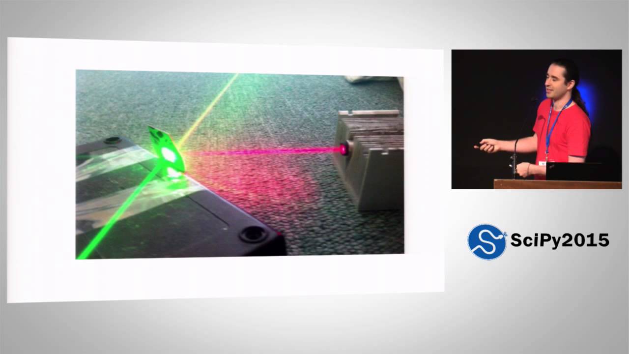
- Because linear combinations are preserved under linear projections, mixing two laser sources (such as a green and red laser to produce yellow) results in a straight line connecting the two points within the XYZ coordinate space.
- The space of all physically realizable human colors is the convex hull formed by the monochromatic laser points along the horseshoe's spectral locus.
---
[08:04](https://www.youtube.com/watch?v=xAoljeRJ3lU&t=484s) How Display Monitors Map to XYZ Space
The linearity of XYZ space simplifies how digital displays are modeled. It is unnecessary to measure the full continuous spectrum emitted by every individual monitor pixel; one only needs to know where the monitor's three primary subpixels (red, green, and blue) land within three-dimensional XYZ space, along with their photon output response. Every display pixel acts as a linear combination of these three primary emitters, creating an internal gamut triangle within the CIE chromaticity slice.
However, mapping computer signals to actual light output is not linear. When a graphics card sends a numerical intensity value (such as 10), the physical display responds along a non-linear power curve. Nathaniel points out the historical baggage behind this behavior: “It's nonlinear because that's how cathode ray tubes work and we now emulate cathode [ray tubes].” Modern monitors continue to simulate the legacy gamma response curves of older analog CRT hardware, meaning software must invert this nonlinearity to achieve accurate photon emissions in real-world displays.
[09:02](https://www.youtube.com/watch?v=xAoljeRJ3lU&t=542s) Modeling Visual Perception and Perceptual Color Spaces
Explaining the final stage of color rendering, the speaker displays a wiring diagram of the visual system in the brain, joking that while each box represents a biological supercomputer, “we don't try to model this.” Instead of simulating the full neural architecture, color scientists rely on curve fitting to match human perceptual behaviors. A fundamental challenge is that light reaching the eye does not map one-to-one to what is consciously perceived. The visual system performs white-point normalization: if it is broad daylight, a relatively bright surface does not appear blinding, whereas in the middle of the night, a bright light appears dazzling. To demonstrate this environmental adaptation, the speaker references the viral dress illusion, noting that “the actual dress in each of these two drawings is identical in terms of the pixels, right?” but appears radically different depending on whether the brain interprets the ambient illuminant as blue shadow or yellowish light.
```mermaid
flowchart TD
accTitle: Color Space Model Progression
accDescr: Progression from raw XYZ spectra to modern uniform color spaces.
subgraph S1["Raw Physical Signal"]
A["Infinite XYZ Cone Space"] --> B["White-Point Normalization"]
end
subgraph S2["Perceptual Modeling"]
B --> C["3D Perceptual Blob"]
C --> D["CIELAB (1976)"]
C --> E["CIECAM02"]
E --> F["CAM02-UCS"]
end
```
In any given scene, white-point normalization chops off the infinite cone of raw CIE XYZ coordinates and rescales them into a finite, three-dimensional perceptual blob. This space is organized with lightness along the vertical axis from black to white, a blue-to-yellow horizontal axis, and a red-to-green cross axis. Computational models have evolved significantly:
* **CIELAB (1976):** A classic model that can be implemented in a single line of Python using the `@` matrix multiplication operator. It incorporates a white-point normalization, a perceptual brightness nonlinearity, and a change of basis. While advanced for the era of desk calculators, it calculates distance-based similarity poorly over short intervals.
* **CIECAM02:** A modern, four-page system of equations providing exceptional hue linearity (ensuring that colors sharing an assigned hue angle actually appear to be the same hue). However, it was not initially built for measuring uniform Euclidean distances.
* **CAM02-UCS:** A uniform color space built by warping CIECAM02 to regularize perceptual distances, incorporating thirty years of color science advances into an accurate model for calculating color differences.
---
[12:09](https://www.youtube.com/watch?v=xAoljeRJ3lU&t=729s) Color Vision Deficiency and Uniformity Metrics
The discussion then turns to color vision deficiency (color blindness). Human color vision relies on rods and three types of cone cells (short, medium, and long wavelength). The medium (green) and long (red) opsins are almost identical because primates acquired the medium cone relatively recently in evolutionary history via a gene duplication. Because these genes remain nearly identical, they frequently recombine or drop out during replication. When an individual has an anomalous or missing red or green cone, their red-green difference channel collapses, effectively squishing their 3D perceptual color space down along that axis.
```mermaid
flowchart LR
accTitle: Colormap Evaluation Pipeline
accDescr: Flowchart showing how VisCM evaluates colormaps across derivatives and colorblind projections.
A["Colormap Trajectory"] --> B["3D Path in CAM02-UCS"]
A --> C["First Derivative (ds/dx)"]
A --> D["Colorblind Simulation"]
C --> E{"Uniform Metric"}
E -->|"Flat derivative"| F["Perceptually Uniform"]
E -->|"Spikes / troughs"| G["Non-Uniform Artifacts"]
```
To analyze how colormaps behave across full vision and deficiency, the team developed a diagnostic visualization tool called VisCM. The tool maps any colormap curve through 3D CAM02-UCS space, places evenly spaced samples along it, and plots the mathematical derivative (the rate of change of perceptual distance). In this framework, “a perceptually uniform color map is one where this line is flat.”
* **Jet:** Jet fails completely; its derivative spikes and crashes, creating false boundaries and masking real gradients while degrading severely under color-blind simulations and grayscale printing.
* **Parula:** Designed for MATLAB to replace Jet, Parula is notably better, but its derivative remains variable. Because Parula was constructed to be uniform in 1976 CIELAB space, it suffers from CIELAB's poor local distance modeling. The speaker emphasizes that “lab space is pretty good for distant colors, about equally good to what we're using, but for nearby colors, it's really terrible.” This mathematical flaw creates a visible, jarring band at the lower end of Parula that, “once is seen, cannot be unseen.”
---
[14:31](https://www.youtube.com/watch?v=xAoljeRJ3lU&t=871s) Designing a Better Colormap: Path Constraints and Bikeshedding
Moving beyond critique, the presenters demonstrate how to synthesize colormaps algorithmically. By defining a trajectory directly inside CAM02-UCS—such as holding lightness constant while tracing a circle in the color plane—one line of Python generates an isoluminant cyclic colormap ideal for directional phenomena like wind shear.
For a general-purpose, sequential default colormap, the physiological constraints dictate the path:
1. **Colorblind accessibility:** The primary trajectory must run along the intact blue-to-yellow axis rather than red-to-green.
2. **Monochrome rendering:** The map must vary monotonically in lightness from dark to light.
3. **Gamut boundaries:** The asymmetric geometry of the color blob dictates traveling from dark blue to light yellow; attempting to go from dark yellow to light blue hits empty gamut space where no physical display colors exist.
Between dark blue and light yellow, two general routes wrap around the perimeter of the gamut. MATLAB's Parula swept along one flank; the team chose the opposing route where there was more volume to maneuver, with Stéfan van der Walt chiming in, “Yeah, we like go to own paths, right?”
To construct paths, they built an interactive GUI where users lock the start and end lightness points, reducing the design problem to a 2D curve manipulated via Bézier control points. However, making colormap creation effortless introduced a new dilemma: “It takes like two minutes to design a new color map. That's terrible because we need a new default color map. And if everyone can design a new color map in two minutes, you will never end up with a single color map because of the problem that if everyone has an opinion, then no decisions can be made.” The team found themselves caught in an open-source bikeshedding trap over display palettes.
---
[16:40](https://www.youtube.com/watch?v=xAoljeRJ3lU&t=1000s) The Matplotlib Survey, Eric Firing, and the Birth of Viridis
To force a decision, the authors produced three distinct candidate palettes and launched an open community poll on the Matplotlib mailing list. The result was inconclusive: “We ran a survey on the map list. We learned that democracy is useless.”
During the debate, core developer Eric Firing asked why none of the candidates featured green. He drafted an alternative path, which the presenters refined. They realized they had overlooked a critical community requirement: “we had left out a very important criterion, maybe the most important criteria in our initial list. That criterion being it has to have green in it.”
With green integrated, the authors unveil their final proposal for Matplotlib's new default colormap: **Viridis** (the Latin word for green). The speaker quips about the name's origins:
* In keeping with Python tradition, it is named after a snake (*Ahaetulla viridis* or green pit viper).
* For those who dislike snakes, it can double as a reference to a bird or a fish.
* For audiences concerned with MATLAB parity, it can also conveniently be interpreted as an avian reference, echoing MATLAB's bird-themed Parula.
Viridis provides wider brightness variation and smoother hue transitions than Parula, eliminating the lower-register artifact kink by leveraging CAM02-UCS mathematics. The presenters announce that Viridis, along with the other candidate colormaps, will be included in the upcoming Matplotlib release.
[18:08](https://www.youtube.com/watch?v=xAoljeRJ3lU&t=1088s) Finalizing Colormaps and the Roadmap to Matplotlib 2.0
Addressing audience reactions regarding the proposed colormap candidates, Nathaniel Smith reassures the crowd that people will still have access to the alternatives if they prefer a different option over the eventual selection: “Like, you can have it. We just need to pick a default.” When an audience member shouts out that the new colormaps need official names, Smith laughs and promises that naming will happen once the designs are set in stone, quipping, “You can't name thing and then kill it, you know.” Furthermore, if the four colormap variants presented are not enough for specific use cases, users can use the underlying framework to build their own.
Looking ahead, Smith outlines the rollout strategy for Matplotlib 2.0, which is scheduled for release in a few months. The major version bump is designed to keep core functionality intact while overhauling visual aesthetics: “It will be exactly the same as the previous release except with better styles, new color map, probably new other things, too.” Recognizing the community's passionate investment in styling choices, Smith jokes, “If you have opinions, I can't imagine anyone here would have opinions, but if you have opinions, we'll have a BoF tomorrow at 1 pm to discuss how Matplotlib should change its defaults to make be better for everyone.” With the invitation extended for the Birds of a Feather session, the speakers wrap up their presentation precisely on schedule.
- **Upcoming Release:** Matplotlib 2.0 will ship within a few months, focusing on refreshed default styling, new colormaps, and visual polish without breaking core capabilities.
- **Community Discussion:** A dedicated Birds of a Feather (BoF) session is scheduled for the following day at 1:00 PM to debate and finalize default styling and colormap choices.
Matplotlib 推出全新默认色图:SciPy 2015 演讲解析
在 SciPy 2015 大会上,Nathaniel Smith 与 Stéfan van der Walt 介绍了为 Matplotlib 打造全新默认色图的历程。传统色图 Jet 因非线性感知容易曲解数据甚至导致误诊,而 MATLAB 的替代方案 Parula 受到版权限制且基于旧版 CIELAB 空间设计。演讲者利用现代色彩科学体系 CAM02-UCS 和诊断工具 VisCM,确立了感知均匀、支持单色打印以及对色觉障碍友好的设计标准。在经历社区讨论并吸纳核心开发者 Eric Firing 引入绿色的建议后,团队最终确定了新默认色图 Viridis,并计划在即将到来的 Matplotlib 2.0 中正式推出。
Smith 指出广泛使用的彩虹色图 Jet 存在严重的感知失真缺陷,甚至在心脏病细胞诊断研究中导致医生出现更多误诊,而 MATLAB 的替代品 Parula 存在版权限制无法直接在开源项目中使用。
团队基于物理光谱投影、三色视觉及 CAM02-UCS 色彩空间确立了设计标准,并开发出诊断工具 VisCM,通过感知距离一阶导数评估色图的均匀性与色盲适应性。
在社区调查并采纳核心开发者 Eric Firing 融入绿色的建议后,团队正式推出新默认色图 Viridis,并宣布该成果与全新默认样式将在 Matplotlib 2.0 中发布。
Reading summary
Nathaniel Smith and Stéfan van der Walt argue that default visualization colormaps act as critical perceptual interfaces whose flaws can lead to severe data misinterpretation, requiring a mathematically uniform replacement engineered around the physics of light and human vision. They introduce Viridis as a new default sequential colormap for Matplotlib to resolve the distortions found in legacy palettes like Jet.
The Severe Perceptual Costs of Default Colormaps (0:00)
Default colormaps serve as the primary visual pipeline translating abstract numerical values into visible structures that the human brain can interpret. However, widely used palettes like Jet introduce severe visual distortions. Smith highlights an empirical study evaluating heart disease diagnostic software based on cell imaging: physicians who used Jet simply because it was the software default insisted they preferred its colorful look, yet empirical testing proved they took twice as long and committed significantly more diagnostic errors compared to using better colormaps.
While MathWorks recognized these flaws and replaced Jet with Parula in MATLAB, proprietary licensing prevents open-source tools from adopting it. Because default colormaps routinely encounter arbitrary datasets without prior domain knowledge, a clean-room open-source default must be sequential rather than diverging or circular, remain aesthetically pleasing to encourage adoption, and preserve accurate perceptual relationships.
Mathematical Foundations of Display and Vision (3:36)
Designing an accurate colormap requires tracing physical light from digital memory to retinal perception. Continuous light spectra represent high-dimensional mixtures of photon counts across wavelengths, bounded by a non-negative cone. Human color perception collapses this infinite dimensionality down to a three-dimensional signal via three types of cone photoreceptors (short, medium, and long wavelengths). This biological projection forms the standard CIE 1931 XYZ color space, where physically distinct spectra that produce identical cone excitations are perceived as metamers. Displays exploit this linearity by using red, green, and blue primary emitters to produce combinations within a chromaticity gamut triangle, though software must invert display gamma power curves emulating cathode ray tubes.
Mapping XYZ signals to conscious perception requires accounting for white-point normalization, where the brain adjusts perceived brightness and color relative to ambient illumination. Classic computational models like 1976 CIELAB normalized white points and brightness, but perform poorly when calculating perceptual distances across short intervals. To accurately measure uniform color steps, the presenters rely on CAM02-UCS, an extension of the CIECAM02 model that warps color space to regularize Euclidean distances based on modern color science.
Evaluating Uniformity and Color Vision Deficiency (12:09)
Human color vision deficiency commonly arises because primate medium (green) and long (red) opsin genes share high sequence similarity and recombine or drop out during replication, collapsing the red-green perceptual axis. To ensure accessibility for colorblind viewers and monochrome printing, an ideal default colormap must vary monotonically in lightness and run primarily along the preserved blue-to-yellow chromatic axis. Furthermore, physical display gamuts are asymmetric; a colormap must traverse from dark blue to light yellow to avoid hitting empty gamut regions lacking physical monitor colors.
To test potential paths against these criteria, the authors developed the diagnostic tool VisCM. The tool maps colormap trajectories through CAM02-UCS space and plots the first derivative of perceptual distance. A perceptually uniform colormap produces a flat derivative line. Jet fails completely, generating abrupt derivative spikes and troughs that create artificial visual boundaries while masking actual data gradients. Even MATLAB's Parula exhibits variable derivatives, causing a visible lower-register banding artifact because it was engineered to be uniform in 1976 CIELAB rather than CAM02-UCS.
Synthesizing Viridis for Matplotlib 2.0 (16:40)
Using Bézier curves inside CAM02-UCS, the presenters engineered candidate paths along the gamut flank opposite Parula's route. However, rapid prototyping exposed an open-source consensus challenge: because colormap generation took only minutes, community surveys produced divided, inconclusive opinions. The design deadlock resolved when core developer Eric Firing noted the absence of green and drafted an alternative trajectory that the authors refined.
The final resulting colormap, named Viridis (the Latin term for green, referencing a snake species in Python tradition), provides wider brightness variation and smoother transitions than Parula without its low-register banding artifact. Viridis, alongside alternative candidate palettes and the VisCM authoring framework, was slated to become the official default in Matplotlib 2.0, providing an aesthetic and perceptual overhaul without disrupting core library functionality.
While Viridis and its companion palettes establish a mathematically verified, accessible standard for general-purpose scientific visualization, Smith and van der Walt emphasize that specialized datasets, such as directional cyclic phenomena, require dedicated colormap trajectories rather than a universal sequential default.
## Background
本内容由 Enthought 频道于 2015 年 7 月 8 日发布在 YouTube 平台上,记录了 SciPy 2015 大会上 Nathaniel Smith 和 Stéfan van der Walt 的演讲。视频简介显示该演讲为 SciPy 2015 大会系列报告与教程的一部分,核心围绕为 Matplotlib 设计更优质的全新默认色彩映射表展开。
## TL;DR
演讲直面了 Matplotlib 长期默认的色彩映射表 Jet 所导致的严重视觉失真与误导性,并从物理光学、视网膜三色感知及人脑知觉模型(CAM02-UCS)出发,系统阐明了感知均匀色彩空间的设计原理。团队克服了传统 CIELAB 空间的局部感知缺陷,针对色盲群体和黑白打印场景设定了几何约束,开发出可精确计算知觉导数的工具。最终,他们打破了开源社区关于审美的“自行车棚效应”争论,正式推出了平滑无伪影的全新默认色图 Viridis,并规划在 Matplotlib 2.0 中全面落地。
## Atmosphere & style
演讲氛围极其轻松幽默且充满自嘲,主讲人 Nathaniel 口才出众、妙语连珠,开场便调侃搭档负责在台上撑颜值,巧妙化解了硬核色彩科学的枯燥感。从列举 Jet 可能造成医疗误诊的严肃现实,到生动拆解大脑视觉处理如同“电闪雷鸣”,再到吐槽开源社区民主决策无用与“自行车棚效应”,整个叙事节奏紧凑而引人入胜。观众在阵阵欢笑中既能感受到严谨的科学推导,又能体会到开源开发者攻克技术顽疾时的纯粹与执着。
## Bulletin
- [00:00](https://www.youtube.com/watch?v=xAoljeRJ3lU&t=0s) 针对旧默认色图 Jet 导致医疗诊断耗时翻倍、误诊率上升等严重感知失真问题,开发团队宣布为 Matplotlib 打造全新的默认色彩映射表方案。
- [09:02](https://www.youtube.com/watch?v=xAoljeRJ3lU&t=542s) 团队规避了 MATLAB 专有色图 Parula 的授权限制,依托现代色彩科学模型 CAM02-UCS 实现了全程导数平直的严苛感知均匀性。
- [14:31](https://www.youtube.com/watch?v=xAoljeRJ3lU&t=871s) 基于贝塞尔曲线交互工具与社区反馈,团队正式推出全新默认色图提案 Viridis,兼顾色盲群体友好性与黑白打印可读性。
- [18:08](https://www.youtube.com/watch?v=xAoljeRJ3lU&t=1088s) 包含 Viridis 及全新默认视觉样式规范的 Matplotlib 2.0 计划在数月内正式上线,四款候选色彩方案均将向社区开放。
## Key takeaways
- [00:00](https://www.youtube.com/watch?v=xAoljeRJ3lU&t=0s) 色彩映射表本质上是数据与人类大脑之间的感知接口,低劣的默认配置会在现实应用(如临床心脏病诊断)中引发显著误诊和效率低下。
- [00:00](https://www.youtube.com/watch?v=xAoljeRJ3lU&t=0s) MATLAB 虽已推出更优的默认色图 Parula,但因商业专有授权限制,开源生态必须从底层独立构建全新的通用解决方案。
- [02:43](https://www.youtube.com/watch?v=xAoljeRJ3lU&t=163s) 通用默认色图的设计标准包括视觉美观、纯顺序型单调结构、数据感知的真实等比例还原,以及对黑白打印和色盲的无障碍支持。
- [04:36](https://www.youtube.com/watch?v=xAoljeRJ3lU&t=276s) 人类视网膜的三类视锥细胞将连续高维光谱投影为三维神经电信号,其线性代数投影构成了 CIE 1931 XYZ 颜色空间的基础。
- [09:02](https://www.youtube.com/watch?v=xAoljeRJ3lU&t=542s) 人脑具备环境光白平衡归一化机制,将物理刺激压缩为包含亮度轴、蓝-黄轴与红-绿轴的三维异形知觉色彩空间。
- [09:02](https://www.youtube.com/watch?v=xAoljeRJ3lU&t=542s) 团队选用最新的 CAM02-UCS 颜色空间,克服了传统 CIELAB 无法准确衡量邻近颜色微小知觉距离的缺陷。
- [12:09](https://www.youtube.com/watch?v=xAoljeRJ3lU&t=729s) 红绿色盲是由于视锥细胞演化重叠与基因变异所致,色图必须沿蓝-黄轴展开并确保感知亮度严格单调递增以保证可读性。
- [12:09](https://www.youtube.com/watch?v=xAoljeRJ3lU&t=729s) 通过对 CAM02-UCS 空间的欧几里得距离求导,可以定量检测色图的感知均匀性;理想色图的导数应呈现水平平直直线。
- [12:09](https://www.youtube.com/watch?v=xAoljeRJ3lU&t=729s) Parula 基于 1976 年 CIELAB 空间优化,导致其感知导数存在明显波动,并在低端暗部留有一道难以忽视的感知明度突变拐点。
- [14:31](https://www.youtube.com/watch?v=xAoljeRJ3lU&t=871s) 开发出交互式贝塞尔曲线生成器后,极低的设计门槛引发了开源社区典型的“自行车棚效应”,最终采纳核心开发者建议引入绿色打破僵局。
- [14:31](https://www.youtube.com/watch?v=xAoljeRJ3lU&t=871s) 全新默认色图 Viridis 沿着深蓝至浅黄路径展开并融入绿相,拥有比 Parula 更平滑的色相过渡和更广的明度跨度。
- [18:08](https://www.youtube.com/watch?v=xAoljeRJ3lU&t=1088s) Matplotlib 2.0 将在保持底层兼容性的同时,全面换装 Viridis 与全新的默认视觉样式,相关设计工具亦支持用户自制感知均匀色图。
## Detailed walkthrough
### [00:00](https://www.youtube.com/watch?v=xAoljeRJ3lU&t=0s) 缘起:Matplotlib 默认色彩映射表与臭名昭著的 Jet
Nathaniel Smith 开门见山地幽默介绍自己和搭档:“I'm Nathaniel. This is Stefan. I'll be doing the talking. He's here to look pretty.”(我是 Nathaniel,这位是 Stéfan。演讲由我来负责,他负责在台上撑颜值。)本次演讲的核心目标,是展示他们如何为 Matplotlib 设计一个全新的默认色彩映射表(colormap),并希望这一成果被官方合并以及被社区广泛采用。
```mermaid
flowchart LR
accTitle: 数据到大脑的视觉通道
accDescr: 展示原始数据通过色彩映射转换后输入人类大脑的过程。
A["数值数据<br/>(无直观意义)"] --> B["色彩映射表<br/>(Colormap)"]
B --> C["RGB 颜色信号"]
C --> D["人脑认知<br/>(识别数据结构)"]
```
色彩映射之所以不可或缺,是因为面对一堆冰冷的裸数据时,肉眼往往难以理出头绪;只有将各个数值映射到对应的颜色,人脑才能瞬间洞察数据背后的拓扑与结构。色彩映射表本质上是“连接数据与大脑的接口”。然而,并非所有色彩映射表都能胜任此职。谈及反面典型,首当其冲的便是让所有人“爱恨交加”的 Jet。Jet 闻名遐迩的原因不仅在于流行,更在于它对数据造成的严重视觉失真。Nathaniel 援引了一项令他印象深刻的研究:科学家对医生利用细胞显微成像诊断心脏病的临床软件展开了用户体验调研。该工具默认采用 Jet,医生们早已习惯于此;在被问及偏好时,医生普遍表示:“Oh yeah, that one. We like it. It's colorful and stuff.”(对,就是那个,我们挺喜欢它,颜色鲜艳。)然而实测数据显示,使用 Jet 时,医生的诊断耗时足足翻倍,而且误诊率显著升高。
> “Like it's a joke but like it's I don't know it may have killed people right like this defaults matter right so so okay not jet but then you have the problem of what do you do instead.” —— Nathaniel Smith
- 默认配置关乎重大:医疗诊断案例表明,低劣的默认色彩甚至可能会在现实中造成致命后果。
- 替代方案的专利困局:MATLAB 在让用户饱受 Jet 折磨多年后,于前一年推出了全新的默认色彩表 Parula(以一种鸟类的学名命名)。Parula 表现良好,但由于商业授权限制,开源界无法直接取用。
- 开源精神驱动:由于拿不到现成可用的优秀方案,开发团队决定从零自研。Nathaniel 自嘲道:“Fine, we'll do it ourselves. How hard can it be? Coincidentally, this slide also explains why it took me seven years to get my PhD.”(好吧,我们自己造。能有多难呢?巧的是,这张幻灯片也正好解释了为什么我花了整整七年才拿到博士学位。)
---
### [02:43](https://www.youtube.com/watch?v=xAoljeRJ3lU&t=163s) 新色彩映射表的设计标准与色彩理论初探
既然要自制全新的默认色彩映射表,团队确立了一组核心设计规范:
1. **色彩丰富且具有美感**:必须色彩鲜艳并且赏心悦目,如果不够美观,用户便不会愿意主动采用。
2. **纯粹的顺序型设计(Sequential)**:作为泛用型默认表,无法预知用户数据的先验特征,因此不能假设数据含有中心发散或循环结构。
3. **忠实呈现数据**:彻底根除 Jet 的失真问题,保证数据数值上的客观变化量,在被人类视觉系统接收后能够引起等比例的主观感知变化。
4. **打印友好性与无障碍设计**:黑白打印时依然清晰可辨,并确保对色盲及弱视群体保持良好的可读性。
为了实现这些技术指标,必须厘清色彩科学。许多人对色彩机制存在认知模糊或误解,Nathaniel 梳理了图像从屏幕抵达大脑的完整物理与生理链条:
```mermaid
flowchart TD
accTitle: 从屏幕显示到大脑感知的物理生理全流程
accDescr: 展现从数值经 RGB、光子、视网膜投射至大脑主观认知的阶段。
subgraph 物理呈现
D1["数据 (Data)"] --> CM["色彩映射表 (Colormap)"]
CM --> RGB["RGB 信号"]
RGB --> M["显示器发射光子"]
end
subgraph 生理感知
M --> R["视网膜感受器 (L/M/S 视锥细胞)"]
R --> E["电化学神经信号 (3D 向量)"]
E --> B["大脑主观色彩感知"]
end
```
针对主观认知形成的末端机制,Nathaniel 诙谐地调侃道:“The photons hit your eye in particular the sensor at the back the retina which creates some electrochemical signal which goes to your brain and then that somehow gets turned into subjective perception by a process involving lightning.”(光子击中眼球后部的视网膜传感器,产生某种电化学信号传输到大脑,接着通过某种伴随着电闪雷鸣的过程转化为感知。)
---
### [04:36](https://www.youtube.com/watch?v=xAoljeRJ3lU&t=276s) 线性感知投影:从无限维光谱到 CIE XYZ 空间
理解视觉机制的第一步是认识光的真实属性。很多人误以为单颗光子的波长数值就代表光本身,但现实中的光源大多由无数不同波长的光子混合而成。除了单波长激光这类特例外,常规光源在数学上表现为定义在各波长光子数量上的极高维(乃至无限维)连续向量。
人类视网膜拥有三类感光视锥细胞(长波 L、中波 M、短波 S)。当高维光谱入射眼睛时,三类细胞相当于对光谱执行内积投影运算,直接输出一个三维向量信号并传递给大脑。这种降维机制具有极佳的线性代数特性:
$$V_{\text{signal}} = \mathbf{P}_{\text{retina}} \cdot \mathbf{S}_{\text{spectrum}}$$
高维空间经由线性变换坍缩至三维空间后,必然产生庞大的高维零空间(null space)。这意味着无数种截然不同的光谱组合(同色异谱现象)能够激发完全相同的三维神经电信号。但在感知工程中,只要两束光谱产生的视神经三维输出等价,就无需追踪其底层光谱的微观差异。这一特性奠定了现代色彩管理的基础——**CIE 1931 XYZ 颜色空间**,它本质上就是为视网膜接收到的三维空间选取的一套基底。
```mermaid
flowchart LR
accTitle: 光谱向 CIE XYZ 空间的线性投影
accDescr: 高维非负光谱空间投影为三维锥体并截面展示为色度图。
A["高维光谱向量<br/>(非负正象限)"] -->|"线性内积投影"| B["3D 信号空间<br/>(三维锥体)"]
B -->|"单形截面 X+Y+Z=1"| C["二维马蹄形色度图<br/>(CIE 1931 Chromaticity)"]
```
- **非负性与锥体结构**:由于特定波长的光子数不可能为负,高维光谱被限制在非负象限内;投影到三维空间后,所有可见颜色便构成一个以原点为顶点的凸锥体。
- **单形截面(Simplex Slice)**:通过在 $X + Y + Z = 1$ 处切出一幅截面,即可获得色彩领域常见的二维马蹄形色度图。该平面的几何外形虽由所选基底决定,但其线性投影性质至关重要。
- **凸包与混合光谱**:单波长激光落在色度图边缘的连续曲线(光谱轨迹)上。将两束激光(如红光与绿光)混合,混合光谱是两者的线性组合;在线性投影保持下,合成色严格落在两点连线之上,从而生成黄色。自然界所有真实色彩的集合,正是这些单色光点所围成的凸包(convex hull)。
对于显示器工程师而言,这一机制带来了极大的便利:显示设备无需模拟大自然的真实连续光谱,每个像素只需包含三颗不同颜色的微型发光单元(RGB),通过调节其发光强度在 XYZ 空间中进行线性混合。屏幕能渲染的所有色彩,完全受限于这三个基色坐标点在色度图内构成的三角形区域(色域)。至于输入信号到实际光子输出强度的非线性响应曲线(Gamma 曲线),Nathaniel 解释道,这完全是因为早期的阴极射线管(CRT)物理特性即是非线性的,而现代显示设备为了保持兼容性,仍在持续模拟 CRT 的响应行为。
### [09:02](https://www.youtube.com/watch?v=xAoljeRJ3lU&t=542s) 人类视觉系统的感知机制与色彩空间演进
在讨论了显示器与发光物理学之后,演讲者指出接下来面对的是人脑视觉系统这一终极环节。虽然物理层面的链路看似简单,但人脑的视觉处理网络由无数复杂的生物计算单元构成,根本无法精确建立微观模型。研究人员采取的方法是“曲线拟合”(Curve Fitting),针对人类关心的具体知觉特性建立足够优秀的近似数学模型。感知到的光线与打入视网膜的光线之间并非一一映射关系,眼睛存在自适应的“白平衡归一化”(White-point Normalization)机制:在大白天看到明亮物体并不觉得刺眼,但在漆黑深夜看到强光就会觉得亮得晃眼。演讲者展示了轰动一时的“蓝黑/白金裙子”视错觉示例,指出两幅图中裙子区域的底层像素其实完全一致,但因为大脑分别假设了不同环境光(蓝光环境 vs. 偏黄光环境),产生了截然不同的颜色认知。
```mermaid
flowchart TD
accTitle: 从三色光到感知色彩空间的处理流程
accDescr: 展示环境光信号经过视网膜视锥细胞与大脑白平衡归一化后,映射至三维知觉色彩空间的流程。
subgraph Retina ["视网膜感光阶段"]
A["外界光信号"] --> B["三类视锥细胞感知 (L, M, S)"]
end
subgraph Brain ["大脑知觉阶段"]
B --> C["环境光白平衡归一化"]
C --> D["三维知觉色彩空间 (CAM02-UCS)"]
end
subgraph Axes ["感知色彩空间三轴"]
D --> E["亮度轴: 黑 ↔ 白"]
D --> F["色度轴 1: 蓝 ↔ 黄"]
D --> G["色度轴 2: 红 ↔ 绿"]
end
```
这种大脑归一化机制将 CIE XYZ 无穷大的视锥空间压缩为一个截断的三维异形感知体(Perceived Colors Blob)。该空间的竖轴代表亮度(黑到白),两个水平轴分别代表蓝-黄维度与红-绿维度。为了在算法中模拟这一知觉空间,色彩科学经历了长足的发展:1976 年提出的经典 CIELAB 空间非常精简,“在即将到来的 Python 3.5 中可以用矩阵乘法运算符一行代码写出来”,当时主要依靠桌面计算器辅助运算;而更先进的 CIECAM02 则包含长达四页纸的复杂方程组。
CIELAB 的初衷是通过欧氏距离来近似色彩相似度,但在色相均匀性上表现欠佳(同一直线上的颜色感知色相并不一致);CIECAM02 在色相准确性上极高,却未针对距离度量优化。因此团队选用了更新的 **CAM02-UCS** 空间,它保留了 CIECAM02 极高的色度准确性,并对其几何空间进行非线性变换以精确匹配知觉色彩距离。正如演讲者所言:
> “So what we're going to be using is this even newer space called CAM02-UCS, which is just built—you start with CIECAM02 and you sort of transform it to make the distances work.”
- CIELAB 包含两层亮度非线性变换:显示器自身的 Gamma 曲线之外,人眼对亮度的感知本身也具有非线性。
- CAM02-UCS 融合了色彩科学近三十年的最新成果,能够同时精确预测人类色相感知与邻近颜色的知觉距离。
---
### [12:09](https://www.youtube.com/watch?v=xAoljeRJ3lU&t=729s) 色盲建模、诊断工具与 Parula 瑕疵剖析
将数据精确映射到大脑感知空间后,还必须兼顾色盲人群的视觉体验。人类视网膜中最常见的三种主要感光细胞中,红绿感光细胞在进化树上分化极晚,是由同一基因复制并发生轻微突变演化而来的,彼此吸收光谱高度重叠。由于序列极度接近,细胞在减数分裂和复制过程中极易发生混淆与重组,导致大多数色盲患者要么这两种细胞的响应曲线变得更接近,要么缺失其中一种。反应在大脑信号层面,红-绿差异信号被大幅削弱甚至抹除,三维色彩空间沿红-绿轴被强烈压缩。
为了全方位审视色图表现,团队开发了一款专门的可视化分析工具。该工具能将任意色图绘制在 3D CAM02-UCS 空间中,均匀采样的数据点如果分布不匀,就意味着感知速度不一致。工具还通过对色彩距离求导,直观展示色图的“感知导数曲线”——一个具备感知均匀性(Perceptually Uniform)的理想色图,其导数曲线应当是一条平直的水平线。在这一检测标准下,老旧的 Jet 漏洞百出:导数剧烈震荡、非均匀性极严重,在色盲与黑白打印模式下完全失效。
```mermaid
flowchart LR
accTitle: 色图知觉导数与均匀性评估
accDescr: 对比理想色图、Jet 与 Parula 在色彩空间导数与知觉均匀度上的表现差异。
A["色彩采样步长"] --> B["CAM02-UCS 空间欧几里得距离"]
B --> C["知觉导数分析"]
C --> D1["理想色图: 导数水平平直 / 无条带伪影"]
C --> D2["Jet: 导数剧烈震荡 / 缺乏感知均匀性"]
C --> D3["Parula: 基于 CIELAB 优化 / 邻近颜色知觉有拐点"]
```
随后演讲者将目光转向 MATLAB 引入的新默认色图 Parula。Parula 相比 Jet 虽有显著提升,但导数曲线上存在肉眼可见的波动,甚至在低端暗部有一道突兀的感知明度拐点(Kink)。演讲者直言:
> “Like there's definitely—once I saw this, you suddenly noticed there's this weird band at the bottom which once is seen cannot be unseen.”
Parula 之所以产生这种肉眼可见的瑕疵,是因为 MathWorks 在设计时是基于 1976 年的 CIELAB 空间进行均匀化优化的。CIELAB 在评估大跨度的远距离颜色时虽然不错,但在预测“邻近颜色间的细微差异”(Nearby Colors)时表现极其糟糕,而保持局部导数平滑正是实现知觉均匀的关键所在。
---
### [14:31](https://www.youtube.com/watch?v=xAoljeRJ3lU&t=871s) 新默认色图设计约束与“给自行车棚挑颜色”的决策困境
既然能精确量化色图表现,也可以反向操作:给定数学约束与几何路径,直接逆向解算出理想的颜色映射。例如设定恒定感知亮度,在水平切面上画一个圆,短短一行调用库的代码背后凝结了上百年的色彩理论成果,即可生成用于展示风向切变或相位变化的环形色图(Circular Colormap)。然而,为 Matplotlib 设计通用的默认色图则面临更严苛的全局几何限制:
1. **色盲友好性**:主色调轴必须沿着“蓝-黄”轴展开,避开红-绿轴;
2. **黑白打印友好性**:感知亮度(Lightness)必须从暗到亮严格单调递增;
3. **空间几何边界**:在知觉色彩空间中,根本不存在“深黄色”到“浅蓝色”的物理实体,唯一的通道是从深蓝走向浅黄。
自顶向下俯视整个色彩几何体,从深蓝到浅黄主要有两条可选的外绕路径。由于 MATLAB 的 Parula 已经选了一条,加上另一侧在色彩空间中有更大的可操作余量,团队决定“走自己的路”,选择反向外绕。
| 评估维度 | 旧默认色图 Jet | MATLAB 默认色图 Parula | Matplotlib 提案 Viridis |
|:--- |:--- |:--- |:--- |
| **设计色彩空间** | RGB 原生渐变 | CIELAB | CAM02-UCS |
| **感知均匀性 (导数)** | 极差,剧烈剧烈震荡 | 较好,但低阶邻近色彩有突兀拐点 | 极高,全程导数曲线平直 |
| **色相与明度设计** | 多色调无序循环 | 蓝-黄主轴,包含绿/黄过渡 | 深蓝至浅黄单调明度递增,融入绿相 |
| **特殊场景兼容** | 红绿色盲失真,灰度打印崩塌 | 兼容色盲与灰度打印 | 完美兼容色盲与黑白打印 |
团队随后开发了贝塞尔曲线交互式色图生成器,支持设定亮度起止点并在二维切面上拖拽控制点,同时实时监控色域裁剪(Gamut),短短两分钟就能设计一款全新的均匀色图。但这却引发了开源社区管理中经典的“自行车棚效应”(Bikeshedding)——当每个人都能在两分钟内造出一套色图时,众口难调的争吵将导致永远做不出决定。
演讲者自嘲地表示,为了打破僵局,他们精选了三款备选方案并发起社区邮件列表投票,结果发现“民主毫无用处(Democracy is useless)”。此时核心开发者 Eric Firing 提出质疑:为什么不把绿色加进去?团队随后引入绿色并经过微调后恍然大悟:原先的技术指标虽然完备,但漏掉了最具决定性的一条感知标准——“里面必须得有绿色”。正如演讲者直率总结道:
> “I don't really care. I just want us to pick something and get rid of Jet.”
```mermaid
flowchart TD
accTitle: 新默认色图 Viridis 的设计与决策历程
accDescr: 展现从技术约束制定、交互设计到社区反馈最终选定 Viridis 的完整闭环。
A["确立核心约束<br/>(深蓝→浅黄 / 亮度单调)"] --> B["开发贝塞尔曲线设计工具"]
B --> C["设计三款初始候选方案"]
C --> D["社区投票陷入'自行车棚'争论"]
D --> E["Eric Firing 提议: 必须包含绿色"]
E --> F["诞生最终方案: Viridis"]
```
最终,团队正式推出了全新的默认色图提案——**Viridis**(拉丁语意为绿色)。为了契合 Python 社区的调性,它以一种绿色的蛇命名(如果不喜欢蛇,也可以当成某种鸟或鱼)。相比于 Parula,Viridis 拥有更大的明度跨度、更柔和的色相过渡,完全消除了 CIELAB 引起的明度突变折痕,并且将在 Matplotlib 的下一个版本中作为全新默认色图全面上线。
### [18:08](https://www.youtube.com/watch?v=xAoljeRJ3lU&t=1088s) 确定默认色图、命名计划与 Matplotlib 2.0 展望
在展示了多款候选色图之后,演讲者针对观众可能出现的偏好分歧进行了说明。大家即便更喜欢第二种方案也没有关系,所有候选方案未来都可以供大家选用,而核心任务只是从中敲定一个官方默认选项。现场有人提出这些候选色图急需正式命名的要求,对此演讲者幽默地安抚道,名字肯定会有的,但目前的策略是先确定最终入选的方案,再正式赋予名称。演讲者开玩笑地表示:“You can't name thing and then kill it, you know.”(你总不能给某个东西起了名字,然后再把它给废弃掉吧)。此外,如果展示的这四种候选色图依然无法满足特定需求,用户完全可以借助他们提供的工具自行生成专属色图。
随后,演讲者公布了项目的后续推进规划:Matplotlib 2.0 预计将在接下来的几个月内正式发布。这个大版本在底层兼容性上将与前一个版本保持一致,主要变化在于带来了更优秀的视觉样式规范、全新的默认色图以及其他一系列默认配置优化。针对开源社区热衷于视觉争议的特点,演讲者打趣说很难想象现场会有人没有自己的看法,因此特别邀请大家参与线下讨论:“If you have opinions, we'll have a BoF tomorrow at 1 pm to discuss how Matplotlib should change its defaults to make be better for everyone.”(如果大家有任何意见或想法,我们明天下午 1 点将组织一场 BoF 专题讨论会,共同探讨 Matplotlib 应当如何调整默认设置,让每个人都能获得更好的体验)。演讲在掌声与准时完赛的轻松氛围中顺利收尾。
- **命名与方案选择**:展示的四款候选色图都将保留供社区使用,团队会在最终敲定默认方案后再为其赋予正式名称,避免过早命名后再将其废弃。
- **自定义色图生成**:配套的代码和算法不仅用于生成候选色图,也支持用户根据感知均匀色彩空间构建专属的新色图。
- **Matplotlib 2.0 发布规划**:新版本将于数月后推出,核心更新聚焦在美化默认样式体系(styles)并正式启用全新的默认色图。
- **社区 BoF 讨论会**:大会次日下午 1 点安排了“Birds of a Feather”(BoF)自由讨论环节,针对 Matplotlib 默认配置改革广泛收集用户与开发者的反馈意见。
## Mentioned
Nathaniel Smith, Stéfan van der Walt, Eric Firing, Matplotlib, Jet, MATLAB, Parula, CIE 1931 XYZ, CIELAB, CIECAM02, CAM02-UCS, Python, Viridis, SciPy 2015, MathWorks
## Video description
Complete SciPy 2015 Talk & Tutorial Playlist here: http://ow.ly/PHjEN
[Source](https://www.youtube.com/watch?v=xAoljeRJ3lU)
Original transcript
[0:00] I'm Nathaniel. This is Stefan. I'll be
[0:02] doing the talking. He's here to look
[0:03] pretty.
[0:08] So, uh, and yeah, we're going to tell
[0:10] you about how we design a new default
[0:11] color map for Map Pot Lib, which we hope
[0:12] they will pick up and how you can too.
[0:15] Um, so, um, color maps, color maps are
[0:19] great because if you have data, you just
[0:21] look at it and it doesn't make any
[0:23] sense. It's just a bunch of
[0:25] I'm sorry, you're not here. Okay.
[0:28] Color maps are great because data
[0:31] doesn't make any sense when you just
[0:32] look at it. But if you take each of
[0:34] those values, map them to some
[0:36] corresponding color, and suddenly you
[0:39] can see the structure that's in your
[0:40] data. Color maps are there. You need
[0:42] color maps because they're an interface
[0:43] between your data and your brain,
[0:44] basically, right? But not all color maps
[0:47] are created equal. Um, for instance,
[0:50] this is everyone's favorite color map
[0:52] they love to hate, Jet. Um, it's famous
[0:55] for how it distorts your data. I won't
[0:58] go into all the long literature about
[1:01] this, but uh, one study I particularly
[1:04] like or if that's the word um, is these
[1:07] people did um, some user studies on a
[1:10] tool for uh, diagnosing uh, heart
[1:14] disease by looking at imaging of cells.
[1:17] So these are doctors looking at patient
[1:19] data. And of course the default in the
[1:22] tool they actually use every day is jet
[1:23] because it's the default color map. Um
[1:26] and so that's what they're practiced at.
[1:28] That's what if you ask them which color
[1:29] map they want to use, they say, "Oh
[1:31] yeah, that one. We like it. It's
[1:32] colorful and stuff." But if you measure
[1:33] their behavior compared to these better
[1:35] color maps over here, they take twice as
[1:37] long and they make more diagnostic
[1:38] errors,
[1:45] right? like it's a joke but like it's I
[1:48] don't know it may have killed people
[1:50] right like this defaults matter right so
[1:53] so okay not jet but then you have the
[1:55] problem of what do you do instead um one
[1:58] sort of obvious thing that might come to
[2:00] mind is this color map called Perula so
[2:02] map lab after inflicting jet on us
[2:05] finally switched away itself like last
[2:07] year to this one um it has a funny sort
[2:10] of name it's because it's named after a
[2:12] bird it's a scientific name and It's a
[2:16] lot better than Jet. It's pretty good.
[2:18] Uh, however, we can't use it because
[2:21] they worked really hard on it, so you
[2:24] can't have it. So, never mind that.
[2:28] Um, I'm sure it's not very good anyway,
[2:30] right?
[2:33] So, we have to make a better one and
[2:34] finest open source project. Fine, we'll
[2:35] do it ourselves. How hard can it be?
[2:38] Coincidentally, this slide also explains
[2:39] why it took me seven years to get my
[2:41] PhD.
[2:42] All
[2:43] right. So, what do we want our new color
[2:46] map? What kind of what are we looking
[2:48] for? So, well, we know it should be
[2:49] colorful. Let's write in the name,
[2:50] right? Um, and probably pretty because
[2:52] if people don't like it, they won't use
[2:54] it. Um, we don't know anything about our
[2:57] data in a default case except that it's
[2:59] like it's numbers, so it should probably
[3:00] just be sequential, not like diverging
[3:02] or circular, any sort of fancier ones
[3:03] that assume structure about the data.
[3:06] And then, of course, the key problem
[3:07] with Jet is we want our new color map to
[3:09] be one that actually accurately
[3:11] represents the data. like if there's a
[3:13] certain change in of the values that
[3:14] should look like that when it hits our
[3:16] brain, right?
[3:18] Be nice for a default in particular if
[3:20] it also works in black and white because
[3:22] people do still print things. Um, and
[3:25] because we are, you know, decent human
[3:26] beings, we want it to be accessible to
[3:28] as many people as possible. So, this is
[3:30] sort of a starting set of criteria. How
[3:31] are we going to do this? These ones down
[3:33] here are tricky because they sort of are
[3:34] involve sort of technical color theory
[3:36] issues. So, let me teach you color
[3:40] theory. The talk is even shorter than I
[3:42] thought, but um so this is just the
[3:45] basics, but it's actually not that
[3:46] complicated. I think people have a lot
[3:48] of like misconceptions and sort of fuz
[3:51] confusion around how color works in my
[3:53] experience. So forget all that. We'll
[3:55] just do it straight from up from the
[3:56] basics.
[3:58] We're scientists, right from the start.
[4:00] What happens when you display something
[4:01] on screen? So you have some data. You
[4:03] put it through color map. You get RGB
[4:05] values. That's a signal goes to the
[4:06] monitor. The monitor spits out some
[4:08] photons. This is what photons look like
[4:11] according to Wikipedia. Um
[4:14] the photons hit your eye in particular
[4:16] the sensor at the back the retina which
[4:18] can creates some electrochemical symbol
[4:21] signal which goes to your brain and then
[4:23] that somehow gets turned into subjective
[4:25] perception by a process involving
[4:26] lightning.
[4:28] So
[4:30] so we need to understand how this
[4:31] process works so we can make sure the
[4:32] data gets to the brain in the correct
[4:34] fashion. Uh the place to start is up
[4:36] here. There's this really nice
[4:38] simplification due to how light works on
[4:40] the retina. Here's the key idea. So, a
[4:42] lot of people think light like a photon
[4:44] has a wavelength. It's just like a
[4:45] number associated with it. But that's
[4:46] not how light is because light is a
[4:48] mixture of lots of photons. So, I mean
[4:51] sure something like my laser pointer
[4:53] here is out of all the different
[4:55] wavelengths, it's just a bunch of light
[4:56] of a single wavelength. But most light
[4:59] sources are you can think of like as
[5:01] these vectors of many many different uh
[5:03] wavelengths and how much how many
[5:05] photonss there are at each one. So very
[5:07] highdimensional kind of thing. And then
[5:10] in the eye there's these three different
[5:11] sensor cell types uh called long,
[5:14] medium, short, 1, two, 3, whatever. Um
[5:17] and basically what happens is the light
[5:19] hits the eye. You take this is like a
[5:21] matrix. You take the you know do dot and
[5:23] you get a threedimensional signal going
[5:25] to the brain, right? And so this is so
[5:27] is really nice because it's linear. So
[5:28] we understand how linear algebra works,
[5:30] right? Um we have this highdimensional
[5:32] space. It's getting projected by a
[5:34] linear option down to operation down to
[5:35] a threedimensional space. So you know
[5:37] there's this highdimensional null space
[5:38] of stuff that's getting collapsed away.
[5:40] It means there's a lot for every
[5:43] possible signal. There's many many
[5:44] possible light sources that generate it.
[5:46] But we don't have to care. We don't have
[5:47] to keep track of those. As long as we
[5:49] know that two different light sources
[5:50] produce the same signal over here,
[5:52] that's all you need to know. So that's
[5:54] sort of the foundation of you know color
[5:56] management in general is it's called the
[5:59] CIExyz space which is picking a nice
[6:02] basis for that threedimensional space.
[6:04] So each point in this threedimensional
[6:06] space represents an equivalence class of
[6:08] spectra. So right here in this
[6:10] visualization I have the three uh
[6:12] coordinate axes. You're sort of looking
[6:14] straight down at the origin.
[6:17] And
[6:18] you think you can't have it's not the
[6:20] case that every single point in the
[6:22] space corresponds to any spectra because
[6:23] you can't have spectra with negative
[6:25] amounts of photons at a particular
[6:26] wavelength. So in the high dimensional
[6:28] space you're restricted to the positive
[6:29] quadrant and that gets projected down to
[6:31] a certain kind like a cone in this space
[6:33] right any along any given line you can
[6:35] either have all the points or none of
[6:36] them and there's sort of a funny shape.
[6:39] So that cone is coming straight out
[6:40] towards us to sort of get a sense of
[6:42] what it looks like. I'm going to take a
[6:43] slice through it at the the simplex the
[6:46] x plus y= z equ= x + y + z equals 1 and
[6:49] on that slice it looks like this. You've
[6:51] probably seen this kind of image before
[6:52] if you spend any time with color. That's
[6:54] what it is. That's where it came from.
[6:56] So how does this work? So for example,
[6:58] here is the spectra of this laser
[7:00] pointer I'm using right now. And it
[7:03] turns out it you project that through it
[7:05] lands right there. If I have a red laser
[7:06] pointer a spectra like this comes over
[7:10] here. And this space has this is sort of
[7:12] arbitrary. We just picked a nice basis
[7:13] that sort of makes it basically they
[7:15] picked a basis that made the shape fill
[7:16] up that triangle. It's it's arbitrary.
[7:18] The space is what matters, not the exact
[7:20] way it's skewed. But the fact that it's
[7:22] linear is very important because so
[7:24] suppose we want to know here's another
[7:25] spectra we can make like by mixing
[7:27] together two laser pointers. Where is
[7:29] that going to end up? Well, that's a
[7:31] linear combination of these two spectra,
[7:33] right? And so if you and linear
[7:35] combinations are preserved under linear
[7:36] projections and so it should end up
[7:39] somewhere on the line between these two
[7:41] projected points. And in fact it does.
[7:44] You get yellow if you put together a
[7:46] green and a red laser.
[7:48] This is the key to understanding why
[7:50] it's shaped like this right is because
[7:52] these kind of laser-like spectra
[7:54] obviously you can make any kind of
[7:55] spectrum out of mixing a bunch of them
[7:57] together. So the space of all possible
[7:59] uh points in this space is the convex
[8:02] hole of those laser-like points. This
[8:04] also tells us how monitors work. Sort of
[8:06] the key point for that. So yeah, that's
[8:08] what light actually looks like. We
[8:11] understand how monitors work. But
[8:12] actually what this means is we don't
[8:14] need to know for a monitor what the
[8:15] actual spectra coming out are. We can
[8:17] just jump straight there. We just need
[8:18] to know for each when we you know send a
[8:21] predictive signal signal to the monitor,
[8:22] which point in that threedimensional
[8:24] space do we end up at? So all we really
[8:26] need to know for each pixel in a modder
[8:28] is basically got three little light
[8:29] bulbs in it. You can think of it. You
[8:30] turn them on more or less strongly. So
[8:32] you mix them together.
[8:34] And what we all we need to know is what
[8:36] are those three points? We're going to
[8:38] take a linear combination of them in XYZ
[8:39] space. And we need to know if we send a
[8:42] particular signal to the monitor, how
[8:43] how much how many photons come out of
[8:45] each one. So for a standard monitor,
[8:48] these are where the three points are
[8:50] located. So that's the space of colors
[8:51] you can actually make. And this is the
[8:54] curve for if you send 10, it sends out,
[8:56] you know, that many photons. It's
[8:57] nonlinear because that's how cathode ray
[9:00] tubes work and we now emulate cathode
[9:02] ray tubes and software.
[9:06] Um, so but this still is pretty simple,
[9:08] right? We're doing pretty well here. We
[9:10] just need to add this one little piece
[9:11] here. No big deal, right? So here's a um
[9:15] a simplified wiring diagram of the
[9:17] visual system in the brain. Each of
[9:19] these little boxes represents a
[9:20] biological supercomput. Um we don't we
[9:24] don't try to model this. Instead we you
[9:26] have some sort of uh um just sort of you
[9:30] basically you do curve fitting. You you
[9:31] come up with some sort of good enough
[9:33] matches to all the different things you
[9:34] the particular sort of perceptual things
[9:36] you care about. Um and so what what is
[9:39] the kind of the space we're trying to
[9:40] figure out? One of the key things that's
[9:42] different about perceived light versus
[9:44] like light that hits your eye is that
[9:46] there isn't a onetoone mapping between
[9:48] uh light hitting your eye and what you
[9:50] end up seeing. A major cause of that is
[9:52] because your eye does some sort you do
[9:54] sort of normalization. Like if it's
[9:56] bright out then you know something
[9:58] that's relatively bright shouldn't look
[9:59] too bright. If it's the middle of the
[10:01] night and you see a really bright light
[10:02] it looks really bright called white
[10:04] spice normalization which produces
[10:07] well-known problems. Right? So if if
[10:09] your brain thinks that there's a blue
[10:11] light here, this looks one thing. If
[10:12] your brain's thinking that there's a
[10:13] sort of yellowish light, it looks
[10:15] different. Right? the actual dress in
[10:18] each of these two drawings is identical
[10:20] in terms of the pixels, right? It just
[10:23] it doesn't look the same because your
[10:25] eye is sort of doing different kinds of
[10:26] correction for the environment. And so
[10:28] what this means is we have that infinite
[10:30] code in XYZ space, but that gets sort of
[10:33] in any given scene there's the brightest
[10:34] thing gets sort of chopped off and you
[10:35] get rescaled into this threedimensional
[10:36] blob is the sort of space of perceived
[10:38] colors. So this is how we think about
[10:40] it. So top to bottom it's like black to
[10:42] white and then there's one axis that's
[10:44] blue to yellow and one that's red to
[10:45] green, right? There's a lot of different
[10:49] sort of computational models of how this
[10:50] works. A classic one many people are
[10:52] familiar with is CIE lab which is
[10:55] literally one line of Python. This is
[10:57] the dot operator coming in Python 3.5.
[11:00] Um so you can see it's you know you
[11:02] normalize the white point. There's a
[11:04] brightness, there's a nonlinearity in
[11:06] our perception of brightness. That's in
[11:07] addition to the one monitors have
[11:08] totally different. And then there's this
[11:11] change of basis thing. Um, this was very
[11:14] fancy in 1976. I assume people were
[11:16] doing this like on their desk
[11:17] calculators. Um, this is sort of the
[11:20] more modern version. It has four pages
[11:21] of equations which I will not try to go
[11:23] through. Um, so compare these. Lab is
[11:28] basically uh designed to estimate
[11:32] similarity by distance.
[11:34] Um, and CKO2 is not, but CKO2 is really
[11:39] excellent at things like, you know, all
[11:40] the all the uh colors along a single
[11:43] line of hue actually are the same color.
[11:45] That's not very true in lab. So, what
[11:48] we're going to be using is this even
[11:49] newer space called Camo2 UCS, which is
[11:52] just built. You start with CMO2 and you
[11:54] sort of transform it to make the
[11:55] distances work. So you keep you keep
[11:57] this nice, you know, nice properties in
[11:59] terms of real really high accuracy
[12:00] another 30 years of development in the
[12:02] science and you get an even better model
[12:04] of color distance as well. So that's
[12:06] that space you were looking at there.
[12:09] Okay. So now we know how all this works.
[12:11] We know how we can go from data. We can
[12:13] run all the way through and figure out
[12:14] what it will look like in the brain. At
[12:16] least for most people. What about people
[12:18] who have color blind? I have to sort of
[12:20] skim through this. Basically remember
[12:22] those four cell types in the eye. people
[12:25] are color blind. Overwhelmingly, what's
[12:27] going on is that there's something a
[12:29] little wonky about one of these two
[12:30] cells. So that the sensors either become
[12:32] more have sort of are even more similar
[12:34] to each other or one is missing
[12:36] entirely. You notice they start out very
[12:38] very similar. It's because we only
[12:40] picked up this middle one very recently
[12:42] in evolutionary time. Um and so it was
[12:45] made by taking a copy of this and
[12:46] tweaking it a little. But this also
[12:48] means it's easy for them to sort of get
[12:49] mixed up during cell replication.
[12:51] Anyway, it's really cool. The effect is
[12:54] that mostly the red green signal is the
[12:56] difference between these two. So um if
[12:59] you take someone who has one of these
[13:01] kinds of anomalies that space gets
[13:03] squished in or more or less along that
[13:06] axis.
[13:08] So okay now we can do this for everyone.
[13:11] And so we built a little tool you can
[13:13] run it yourself to help us you know
[13:15] visualize how color maps work. You see
[13:17] there's the color map itself and here it
[13:19] is in 3D space. The little dots are
[13:21] equally spaced here. So you can see that
[13:22] it's not very uniform. And another way
[13:24] to visualize that is we've just taken
[13:25] like the derivative basically. So a
[13:27] perceptually uniform color map is one
[13:29] where this line is flat. Jed is not
[13:31] perceptually uniform.
[13:33] And then down here you have what it
[13:35] looks like to color blind people
[13:36] hopefully approximately um and for black
[13:40] printing and some examples. Right there
[13:42] it is jet. It's terrible. Um we can also
[13:45] look at like perula. Um there's
[13:47] something interesting going on here. So
[13:48] you can see it's a lot better than jet,
[13:50] right? It's a little bit variable here.
[13:52] But notice that the axis there is that's
[13:54] 200 and over here 200's down here. So
[13:57] that's actually much more variable. You
[13:59] can see it isn't perfect at all though.
[14:01] Like there's definitely once I saw this,
[14:03] you suddenly noticed there's this weird
[14:05] band at the bottom which once is seen
[14:07] cannot be unseen. It's even stronger on
[14:09] a monitor than on this screen. Um,
[14:12] what's going on here is that PULA they
[14:13] designed to be perfectly uniform in lab
[14:15] space.
[14:18] And it turns out lab space is pretty
[14:20] good for distant colors, about equally
[14:21] good to what we're using, but for nearby
[14:23] colors, it's really terrible. And that's
[14:26] the crucial thing for uniformity is
[14:27] getting those nearby color estimates,
[14:29] right? So we can also do is we not
[14:32] restricted to just saying like, okay,
[14:34] here's a color map. How does it look? We
[14:35] can say, here's what we want it to look
[14:36] like. Give me that color map. So we made
[14:38] it. So here's a example of how you can
[14:40] do that. Say you want to make a little
[14:42] circular color map. Say well okay I want
[14:43] the same lightness at every point and I
[14:46] want then I'll draw a little circle in
[14:47] the other plane and then I said those
[14:51] are my coordinates. Please convert using
[14:53] our little library. There's like a
[14:55] hundred years of color theory in that
[14:56] line of code and you get these neat
[14:59] things. So here's wind directions. You
[15:00] can see sort of where there's shear
[15:02] between two different Anyway, it's fun.
[15:04] I need to move on. What about a default
[15:06] color map?
[15:08] um for our default color map. So we know
[15:10] to be colorb blind friendly we have to
[15:12] use blue yellow as our main axis not red
[15:14] green and to be grayscale friendly we
[15:16] need to go from sort of dark to light.
[15:19] Uh and that means that we want to go
[15:21] from dark blue to light yellow because
[15:22] you try to go from dark yellow to light
[15:24] blue. It does there there's nothing
[15:25] there. It's just how the blob is shaped.
[15:27] So we're pretty constrained. Um our main
[15:30] choice that's left is here we're looking
[15:31] down on the blob from the top. We're
[15:33] trying to get from here to here. We
[15:34] could kind of go around that way or we
[15:35] could kind of go around that way.
[15:37] Now, we thought, well, Mat Lab went
[15:38] around that way, plus there's sort of
[15:40] more room to work on here, so it's just
[15:41] better to go this way.
[15:44] Yeah, we like go to own paths, right?
[15:47] Yeah, exactly. Um, so we made a little
[15:49] tool to do this. I am sorry, Stefan. I
[15:52] think we are cutting a little bit short
[15:55] the uh your demo portion here. So, this
[15:56] is the tool. I know, but I we're already
[15:59] out of time. Like
[16:02] um so you at the bottom you can choose
[16:05] the where to start and end and light
[16:08] lightness brightness. And since that
[16:10] totally determines that axis, then you
[16:11] can only you only have to deal with the
[16:12] 2D top down view over here. And you just
[16:14] draw these drag these bezier points
[16:16] around to change this. You can also look
[16:18] at different slices to make sure you're
[16:19] staying in gamma. It's great. It takes
[16:21] like two minutes to design a new color
[16:23] map. That's terrible because we need a
[16:26] new default color map. And if everyone
[16:28] can design a new color map in two
[16:29] minutes, you will never end up with a
[16:30] single color map because of the problem
[16:32] that if everyone has an opinion, then no
[16:34] one no decisions can be made. And here
[16:36] we are literally trying to decide what
[16:37] color to make the bike shed.
[16:40] So our solit strategy, we made three. So
[16:43] that's enough people have an opinion,
[16:44] but not so many it gets out of control.
[16:46] And what we we ran a survey on the map
[16:48] list. We learned that democracy is
[16:50] useless.
[16:53] At the same time, um, Eric Firing said,
[16:56] "Well, but why don't we put green in?"
[16:58] And he said, "Okay, fine." He designed
[17:00] one, we tweaked a little. Um, and we
[17:01] learned that, in fact, we had left out a
[17:03] very important criterion, maybe the most
[17:05] important criteria in our initial list.
[17:07] That criterion being it has to have
[17:09] green in it.
[17:15] [Applause]
[17:17] So,
[17:19] I don't really care. I just want us to
[17:21] pick something and get rid of jet. So,
[17:23] let me present our proposal for Mapot
[17:25] Lib's new color map. We're calling it
[17:26] Virus. That's Latin for green. Of
[17:29] course, this is Python. It's because
[17:30] it's named after it's really named after
[17:31] a snake. If you don't like snakes, you
[17:33] could pretend it's named after a bird or
[17:35] a fish. Or if you're in a context where
[17:37] Mat Lab compatibility is very important,
[17:39] then it could also be named after a
[17:40] bird.
[17:43] Compared to Perula, um, we have more
[17:46] brightness variation, less hue
[17:48] variation. Um, I like it better.
[17:54] You're allowed to use it.
[17:56] Uh, and it has and it avoids sort of
[17:58] that annoying kink. It's a more fancy
[18:00] sophisticated model. And so, where are
[18:03] we now? All of our color maps will be
[18:06] available in the next release. So,
[18:07] please don't come and tell me. No, no,
[18:08] no. You should have chosen the second
[18:09] one instead. Like, you can have it. We
[18:11] just need to pick a default.
[18:13] Um, if if the what?
[18:15] We need names.
[18:16] We'll give them names. It's fine. There
[18:18] will be names. I just we want to like
[18:21] get it finalized before we give names to
[18:23] things, right? You can't name thing and
[18:24] then kill it, you know. Yeah. Um
[18:27] and if those four aren't enough, you can
[18:30] make your own. Just let's fix one, too.
[18:33] Um so, you know, so here's what's going
[18:35] on. The plan is Matt Lab Mattplot Lib
[18:38] 2.0 is coming out in a few months. It
[18:39] will be exactly the same as the previous
[18:41] release except with better styles, new
[18:43] color map, probably new other things,
[18:45] too. If you have opinions,
[18:48] I can't imagine anyone here would have
[18:50] opinions, but if you have opinions,
[18:52] we'll have a bof tomorrow at 1 pm to
[18:54] discuss how map liib should change its
[18:56] defaults to make be better for everyone.
[18:58] Come and do that. Yes. Thank you.
[19:04] Right on time.