D/A and A/D | Digital Show and Tell (Monty Montgomery @ xiph.org)

FL Studio

AI-assisted summary of D/A and A/D | Digital Show and Tell (Monty Montgomery @ xiph.org) — original source. Check the original for full context.

Source published: 2013-03-02

Key ideas

Digital-to-analog conversion does not produce a stair-step signal; under the Nyquist-Shannon sampling theorem, band-limited discrete samples yield exactly one mathematically continuous analog curve. (5:58)
Bit depth determines the dynamic range and noise floor rather than waveform smoothness, with 16-bit audio outperforming professional analog reel-to-reel tape systems that peaked near 13 bits of effective resolution. (8:45)
Applying dither during quantization decouples quantization error from the input signal, replacing harmonically correlated distortion with flat, predictable noise and allowing signals below half a bit to be preserved perfectly. (12:23)
Digital systems are not bound to a timing resolution limited by the sample period; band-limited signals faithfully preserve sub-sample transient timing and reconstruct edges at arbitrary points between samples. (20:53)

Detailed notes

## Background Published on March 2, 2013, on YouTube by FL Studio, this video features Monty Montgomery from Xiph.org demonstrating digital audio principles. According to the page description, the presentation uses real audio gear, modern digital analysis, and vintage analog bench equipment to address the digital versus analog quality debate, explaining why 16-bit, 44.1 kHz digital signals reproduce audible sound with complete fidelity.

## TL;DR Monty Montgomery dismantles enduring digital audio myths by testing real signals through an analog-digital-analog loop using vintage analog laboratory equipment. He disproves the common "stair-step" misconception by demonstrating that band-limited discrete samples reconstruct into perfectly smooth continuous sine waves up to 20 kHz. The presentation explores how bit depth governs noise floors rather than geometric resolution, showing how dither eliminates harmonic distortion and preserves signals smaller than a single bit. Montgomery also clarifies the nature of band-limiting and Gibbs phenomenon ripples on square waves, proving that digital systems possess infinite sub-sample timing resolution rather than time-stepped limitations.

## Atmosphere & style The presentation carries the cozy, delightfully nerdy warmth of a late-night workbench session guided by a seasoned engineer who loves taking things apart. Montgomery's delivery is humble, dryly humorous, and reassuringly unpretentious, swapping audiophile mysticism for concrete oscilloscope traces and clunky vintage gear. Watching the green CRT phosphor lines smoothly track waveforms feels deeply satisfying, transforming abstract signal theory into an intuitive, visually conclusive reality check.

## Bulletin - [05:58](https://www.youtube.com/watch?v=cIQ9IXSUzuM&t=358s) Digital-to-analog conversion does not produce a stair-step signal; under the Nyquist-Shannon sampling theorem, band-limited discrete samples yield exactly one mathematically continuous analog curve. - [08:45](https://www.youtube.com/watch?v=cIQ9IXSUzuM&t=525s) Bit depth determines the dynamic range and noise floor rather than waveform smoothness, with 16-bit audio outperforming professional analog reel-to-reel tape systems that peaked near 13 bits of effective resolution. - [12:23](https://www.youtube.com/watch?v=cIQ9IXSUzuM&t=743s) Applying dither during quantization decouples quantization error from the input signal, replacing harmonically correlated distortion with flat, predictable noise and allowing signals below half a bit to be preserved perfectly. - [20:53](https://www.youtube.com/watch?v=cIQ9IXSUzuM&t=1253s) Digital systems are not bound to a timing resolution limited by the sample period; band-limited signals faithfully preserve sub-sample transient timing and reconstruct edges at arbitrary points between samples.

## Key takeaways - [03:39](https://www.youtube.com/watch?v=cIQ9IXSUzuM&t=219s) Analog test equipment reveals that digital signals converted back to analog emerge as continuous, smooth waveforms without stair steps, even up to the 20 kHz limit of human hearing. - [05:58](https://www.youtube.com/watch?v=cIQ9IXSUzuM&t=358s) Sampled digital signals are discrete-time values with no defined state between sample intervals; stair steps exist solely as software visualization conventions or intermediate zero-order hold states. - [05:58](https://www.youtube.com/watch?v=cIQ9IXSUzuM&t=358s) The Nyquist-Shannon sampling theorem guarantees that exactly one continuous band-limited waveform can pass through a set of discrete samples below half the sampling rate. - [08:45](https://www.youtube.com/watch?v=cIQ9IXSUzuM&t=525s) Sampling itself is mathematically lossless; quantization is the step that introduces noise by limiting amplitude precision to discrete levels. - [08:45](https://www.youtube.com/watch?v=cIQ9IXSUzuM&t=525s) Quantization noise behaves identically to analog magnetic tape hiss when using Gaussian dither, revealing that consumer cassette tapes possessed only 5 to 9 bits of dynamic range. - [12:23](https://www.youtube.com/watch?v=cIQ9IXSUzuM&t=743s) Truncating without dither causes quantization errors to correlate with the input signal, generating harmonic distortion spikes that rise above the flat noise floor. - [12:23](https://www.youtube.com/watch?v=cIQ9IXSUzuM&t=743s) Dither enables the complete preservation of sub-bit signals (such as 0.25 LSB), which would otherwise collapse to complete silence and 100% distortion through truncation. - [14:08](https://www.youtube.com/watch?v=cIQ9IXSUzuM&t=848s) Noise shaping shifts dithering energy out of the human ear's most sensitive 2 kHz to 4 kHz range and into higher frequencies, making dither perceptually quieter. - [14:08](https://www.youtube.com/watch?v=cIQ9IXSUzuM&t=848s) While shaped dither increases overall RMS noise power compared to unshaped truncation error, psychoacoustic curves ensure it sounds substantially quieter to the human ear. - [14:08](https://www.youtube.com/watch?v=cIQ9IXSUzuM&t=848s) At 16 bits, undithered distortion artifacts and dither noise sit roughly 100 dB below full-scale peaks, making dither a subtle safeguard rather than a catastrophic audio defect. - [17:23](https://www.youtube.com/watch?v=cIQ9IXSUzuM&t=1043s) Gibbs phenomenon ringing on square waves is an inescapable mathematical consequence of band-limiting above 20 kHz, not a distortion introduced by filter defects. - [17:23](https://www.youtube.com/watch?v=cIQ9IXSUzuM&t=1043s) Passing an already band-limited signal through an anti-aliasing low-pass filter a second time produces zero additional ripple or degradation. - [20:53](https://www.youtube.com/watch?v=cIQ9IXSUzuM&t=1253s) Digital audio timing resolution is continuous rather than quantized to sample intervals, allowing transitions and transients to be placed accurately between individual samples.

## Detailed walkthrough ### [00:03](https://www.youtube.com/watch?v=cIQ9IXSUzuM&t=3s) The Stair-Step Myth and Vintage Analog Bench Gear

Monty Montgomery introduces the motivation behind the demonstration: a few months prior, he authored an article examining digital audio and explaining why 24-bit/192 kHz audio downloads make little practical sense. In passing, the article mentioned that a digital waveform is not a stair step and that converting digital back to analog does not produce stair steps. Surprisingly, that single passing remark triggered the vast majority of feedback. Over half of the correspondence he received involved fundamental questions and confusion surrounding basic digital signal behavior. To clear up these misconceptions from first principles, Monty designs an experiment assuming the audience knows nothing about how digital signals behave—meaning digital test equipment cannot be trusted either.

To observe the signals purely through an analog lens, Monty sets up a workbench filled with vintage analog laboratory equipment. An HP 3325 synthesizer/function generator from 1978 serves as the analog signal source; Monty jokes that while it is heavy, bulky, power-hungry, and equipped with a loud cooling fan, units can still be found on eBay for barely more than the shipping cost. Signals are monitored in the time domain using a Tektronix 2246 oscilloscope from the mid-1990s—one of the finest analog scopes ever built. Frequency content is tracked via an HP 3585 analog spectrum analyzer. While these instruments contain large, rudimentary microcontrollers, the actual signal paths from physical input to CRT screen remain entirely analog.

- **Signal baseline:** The HP 3325 outputs a clean 1 kHz sine wave at 1 V RMS (2.8 V peak-to-peak), confirmed identically across the Tektronix scope and the HP 3585 spectrum analyzer. - **Spectrum baseline:** The analyzer reveals a trace of low-level white noise and minor harmonic distortion, with the highest harmonic peak roughly 70 dB below the fundamental frequency.

```mermaid flowchart LR accTitle: Analog and Digital Signal Flow accDescr: Diagram tracing the signal from the analog generator through conversion and back to output scopes. subgraph Input ["Analog Source"] A["HP 3325 Generator"] --> B["Input Scope & Spectrum Analyzer"] end subgraph Digital ["Digital Loopback"] B --> C["Edirol USB Interface (A/D)"] C --> D["ThinkPad Display"] D --> E["Edirol USB Interface (D/A)"] end subgraph Output ["Analog Output"] E --> F["Output Tektronix Scope"] end ```

[02:43](https://www.youtube.com/watch?v=cIQ9IXSUzuM&t=163s) Inserting the Digital Conversion Loop

To examine digital conversion, Monty places an older consumer-grade Edirol USB audio interface (more than ten years old) into the middle of the signal chain. He points out that while modern converters boast specifications an order of magnitude superior in linearity, jitter, flatness, and noise floor, human hearing cannot distinguish those measured gains because even older budget interfaces already operated right at the boundary of audible transparency. The interface feeds an analog signal into a ThinkPad laptop to display digital waveform data and fast Fourier transform (FFT) spectra, then immediately routes that digital stream back out of the interface's D/A stage for display on the analog output oscilloscope.

Monty stresses the fundamental transparency of standard consumer gear: “Just because we can measure an improvement doesn't mean we can hear it, and even these old consumer grade boxes were already at the edge of ideal transparency.”

[03:39](https://www.youtube.com/watch?v=cIQ9IXSUzuM&t=219s) Sweeping from 1 kHz to 20 kHz: The Disappearing Steps

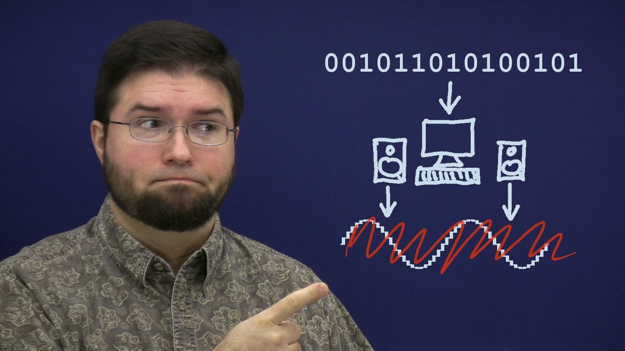
The experiment begins by digitizing the 1 kHz sine wave to 16-bit PCM at 44.1 kHz—identical to standard CD audio format. On the ThinkPad screen, the software visualization renders the digitized sine wave as a classic stair-step pattern, dedicating one horizontal block per sample. Yet when the signal emerges from the D/A converter and appears on the analog output scope, it is an identical, pristine, continuous sine wave with zero stepping.

To test whether the 1 kHz signal is merely so oversampled that steps are too fine to see, Monty increases the generator frequency toward the Nyquist frequency. At 15 kHz, the wave is captured with fewer than three samples per cycle, causing the digital stair-step drawing on the laptop screen to look crude and distorted. On the analog oscilloscope, however, the output remains a clean sine wave. Stepping the frequency up through 16 kHz, 17 kHz, 18 kHz, 19 kHz, and finally to 20 kHz—the absolute upper limit of human hearing—the analog output scope continues to trace an uncorrupted, perfectly smooth sine wave with no level drop-off or jagged edges.

- **Digitization parameters:** 16-bit linear PCM at a 44.1 kHz sample rate. - **Waveform fidelity:** At 20 kHz (fewer than 2.25 samples per cycle), the reconstructed analog output displays zero jaggedness, rounding, or amplitude attenuation.

[05:58](https://www.youtube.com/watch?v=cIQ9IXSUzuM&t=358s) Discrete-Time Sampling vs. Continuous Stair Steps

Monty asks where the stair steps went, revealing it is a trick question: “So where'd the stair steps go? Don't answer; it's a trick question: they were never there.” A stair-step signal is a continuous-time function that maintains an explicit, defined value at every single instant between changes. A digital sampled signal, by contrast, is strictly discrete-time. It possesses values only at instantaneous sample points and is completely undefined at every instant in between. A discrete-time signal is properly represented mathematically as a lollipop graph, not a staircase.

According to the Nyquist-Shannon sampling theorem, when a continuous signal is band-limited to below half the sampling rate (the Nyquist frequency), there is exactly one continuous curve that can pass through all of those discrete sample points. While someone could hand-draw alternative paths connecting the points, any path differing in the slightest degree from the original must incorporate frequencies at or above Nyquist, thereby violating the band-limiting criterion. The original input waveform is the sole valid mathematical solution.

Monty identifies two primary reasons why the stair-step misconception persists: 1. **Zero-Order Hold stages:** Simple digital-to-analog converters often hold an instantaneous voltage level until the next sample arrival as an intermediate step (a zero-order hold). While textbooks and diagrams often show this stepped intermediate stage, it is not a finished conversion and never reaches the final output unchanged. 2. **The "Fat Bits" visualization habit:** Engineers draw stair steps for digital samples much like image editors render pixels as little square boxes ("fat bits"). Pixels are mathematically points sampling a continuous two-dimensional space without volume or shape; rendering them as tiny squares is merely an editing convenience because viewing infinitely small points is impractical.

[08:45](https://www.youtube.com/watch?v=cIQ9IXSUzuM&t=525s) Bit Depth, Quantization, and Tape Hiss

Monty demonstrates that bit depth has no bearing on waveform smoothness. To prove this, he routes the same sine wave through a second channel quantized with dither down to a coarse 8 bits. Observed on the analog oscilloscope, Channel 2 displays a smooth, uninterrupted sine wave rather than a jagged, stepped signal. The only visual difference is the presence of slight trace fuzz, indicating an elevated noise floor.

Quantization affects signal-to-noise ratio rather than signal geometry. Monty explains the distinction: “When we digitize a signal, first we sample it; the sampling step is perfect, it loses nothing. But then we quantize it, and quantization adds noise.” The number of bits determines only the depth of that noise floor.

When Monty isolates Channel 2's noise by applying a notch filter to strip out the fundamental sine wave and raising the monitor gain, the audible result is identical to steady analog tape hiss. When using Gaussian dither, the quantization noise is mathematically equivalent to magnetic tape noise. This equivalence allows the noise floor of magnetic tape formats to be stated directly in bits: - **Standard compact cassettes:** Peak performance reached roughly 9 bits of dynamic range under pristine conditions, but 5 to 6 bits was typical for home consumer decks and mixtapes. - **Professional studio open-reel tape:** State-of-the-art studio reel-to-reel machines using advanced noise reduction systems (such as Dolby SR) barely attained 13 bits of effective resolution. - **The "DDD" CD marker:** The historical "DDD" label on early compact discs was considered an elite audiophile achievement because purely digital recording and mastering bypassed the severe 13-bit ceiling of tape.

[11:39](https://www.youtube.com/watch?v=cIQ9IXSUzuM&t=699s) The Mechanism and Purpose of Dither

Addressing why he specifically refers to quantizing *with dither*, Monty defines the alternative: simple truncation or rounding. In basic quantization, the converter simply selects the nearest discrete digital amplitude level to the incoming analog voltage. While mathematically straightforward, the rounding errors that result correlate directly with the input waveform. This correlation generates harmonically related distortion and unnatural, program-dependent artifacts rather than benign white background noise.

Dither solves this issue by introducing a small, carefully tailored noise signal during quantization. Rather than masking or burying distortion under an added layer of sound, dither randomizes the quantization intervals, completely decoupling quantization error from the input signal. In doing so, it replaces harmonically correlated distortion with an entirely benign, predictable, stationary noise floor of chosen characteristics.

[12:23](https://www.youtube.com/watch?v=cIQ9IXSUzuM&t=743s) Dither: Converting Harmonic Distortion into Linear Noise

Because the analog hardware signal generator introduces too much inherent noise for a delicate quantization test, Monty switches to generating a mathematically synthesized, pristine sine wave on his ThinkPad. Quantizing this pure tone to 8 bits with dither turned on reveals a clean sine wave on both the digital waveform display and the analog oscilloscope. Once the sweeping analog spectrum analyzer catches up, both the digital and vintage analog spectral displays show a sharp, pristine frequency spike resting above a completely uniform, flat noise floor.

```mermaid flowchart TD accTitle: Quantization with and without Dither accDescr: Diagram contrasting how dither converts correlated harmonic distortion into uncorrelated flat noise, and preserves sub-bit signals.

subgraph DitherON["With Dither Enabled"] A1["Quantization to 8 bits"] --> B1["Noise randomized and decorrelated"] B1 --> C1["Flat, uniform noise floor"] C1 --> D1["Signals < 0.5 LSB preserved perfectly"] end

subgraph DitherOFF["Without Dither (Truncation)"] A2["Quantization to 8 bits"] --> B2["Quantization error correlates to signal"] B2 --> C2["Harmonic distortion peaks rise above noise"] C2 --> D2["Signals < 0.5 LSB quantize to absolute zero"] end ```

The moment dithering is switched off, the behavior changes completely. The quantization noise that dither had spread into an innocuous, broadband hiss collapses and concentrates into jagged harmonic distortion spikes. Although the baseline noise floor technically drops lower, the distortion becomes non-zero, with harmonic peaks protruding significantly higher than the dither noise ever reached. At 8 bits, this distortion is visibly prominent, whereas at 16 bits, undithered harmonic distortion drops to levels so low as to be completely inaudible in ordinary listening. As Monty observes regarding audio processing: “Still we can use dither to eliminate it completely if we so choose.”

Dither also completely rescues low-amplitude signals from disappearing. Without dither, the absolute level of quantization distortion remains roughly constant regardless of input amplitude; however, once the signal level drops below half a bit, every sample quantizes to zero, creating total signal loss. As Monty puts it, “In a sense everything quantizing to zero is just 100% distortion.” Re-enabling dither instantly resurrects a tone measuring only one-quarter of a bit, rendering it clearly discernible above the flat noise floor.

- **Test Signal**: Pure sine wave generated mathematically on an IBM ThinkPad, quantized down to 8 bits. - **Spectrum Behavior**: Dither creates a flat, uniform noise floor; turning dither off creates discrete harmonic distortion spikes. - **Sub-bit Performance**: A 0.25-bit (one-quarter LSB) sine wave is completely eliminated by truncation, but fully preserved and recoverable when dither is active.

---

[14:08](https://www.youtube.com/watch?v=cIQ9IXSUzuM&t=848s) Noise Shaping and Dither Power Trade-offs

Because dither is an artificial noise added intentionally, its spectral shape does not have to remain white or flat. Human hearing is acutely sensitive to mid-range frequencies between 2 kHz and 4 kHz, making background hiss in that band particularly intrusive. By employing noise shaping, the energy of the dithering noise is shifted out of the ear's most sensitive mid-range and pushed into the highest audible frequencies where human hearing is far less perceptive. While 16-bit dither noise is ordinarily far too faint to hear, boosting the monitor gain enormously makes the difference obvious, demonstrating how noise shaping effectively vanishes into the background compared to unshaped noise.

Total dithered quantization noise possesses a higher overall root-mean-square power than raw undithered quantization error, which can be seen fluttering on a VU meter during passages of near-silence. Dither is not merely a binary toggle; engineers can reduce dither power to strike a calculated balance between a lower noise floor and minor harmonic distortion. Modulating the amplitude of an input signal demonstrates this interaction: at full dither power, the noise floor remains rock-steady, uniform, and completely uncorrelated with the input signal. As the dither power is dialed back, the modulating input begins to audibly modulate the noise floor itself, producing signal-dependent noise chatter. Noise shaping offers an added benefit here, requiring somewhat less dither power before the input signal begins to audibly modulate the output noise.

Monty steps back to place the entire dither debate into practical engineering perspective. All of these subtle adjustments involve artifacts and noise floors that sit 100 dB or more below full scale. If the Compact Disc standard had frozen at the original 14-bit proposal from early digital development, aggressive dithering would have been vital; at 16 bits, it operates largely as an insurance policy providing a few extra decibels of dynamic range. Monty emphasizes that creative priorities should remain paramount, remarking, “The simple fact is though no one ever ruined a great recording by not dithering the final Master.”

- **Ear Sensitivity Range**: 2 kHz to 4 kHz is the most sensitive band for human hearing, making it the primary region to clear via noise shaping. - **Noise Power vs. Perception**: Shaped dither contains higher total energy than flat truncation noise, yet sounds markedly quieter due to psychoacoustics. - **Dynamic Floor Context**: At 16 bits, dithering effects occur 100 dB below full-scale signal peaks.

---

[17:23](https://www.youtube.com/watch?v=cIQ9IXSUzuM&t=1043s) Square Waves, Band Limiting, and the Gibbs Phenomenon

Moving past simple sine waves, Monty feeds a 1 kHz square wave from the signal generator into the ADC to examine complex waveforms. When viewed on the oscilloscope, the input is a sharp, two-level square wave, but the analog output oscilloscope reveals distinct ripples flanking every sudden level transition. A mathematical square wave is defined as a fundamental frequency summed with an infinite series of odd harmonics. However, real-world digital audio systems do not possess infinite bandwidth; an anti-aliasing filter sharply truncates all energy above 20 kHz.

```mermaid flowchart LR accTitle: Gibbs Effect in Band-Limited Audio accDescr: Flow showing how sharp anti-aliasing removes odd harmonics to create Gibbs ripples, which do not worsen on subsequent filtering passes.

A["Analog 1 kHz Square Wave (Infinite Odd Harmonics)"] --> B["Anti-Aliasing Filter (Cuts off at 20 kHz)"] B --> C["Band-Limited Square Wave (Exhibits Gibbs Ripples)"] C --> D["Second Filter Pass (Same 20 kHz cutoff)"] D --> E["Identical Waveform (Only slight phase/fractional delay)"] ```

Slicing away all harmonics above 20 kHz inevitably transforms the square wave into a band-limited wave containing Gibbs phenomenon ripples around the transitions. A widespread myth asserts that these ripples are nasty distortion artifacts continuously introduced by anti-aliasing and reconstruction filters, implying that each filter pass will compound the ringing. To test this, Monty patches the already-filtered signal through the sharp filter a second time. Outside of introducing a fractional-cycle propagation delay, the waveform does not change at all. As Monty summarizes: “A second pass can't remove frequencies that we already removed.”

Gibbs ripples are not active filter defects; they are the fundamental mathematical definition of a band-limited signal. Even if a user draws a synthetic square wave in digital audio software that appears perfectly rectangular because its transitions line up cleanly with individual sample points, that clean appearance is an illusion created by "connecting the dots." Beneath those samples, the unique band-limited analog signal represented by those points still contains the exact same Gibbs ripples.

- **Harmonic Composition**: A square wave consists strictly of odd harmonics ($f, 3f, 5f, 7f, \dots$) decreasing in amplitude. - **Filter Cutoff**: The ADC's anti-aliasing filter removes all harmonic energy above 20 kHz. - **Gibbs Phenomenon**: Ringing at edges occurs naturally whenever a continuous spectrum is truncated while non-zero energy remains. - **Multi-pass Filter Test**: Sending a band-limited signal through the identical low-pass filter a second time produces zero additional ripple.

---

[20:53](https://www.youtube.com/watch?v=cIQ9IXSUzuM&t=1253s) Timing Precision Between Samples

Another widespread misconception about digital audio is that its timing precision is constrained by the sample period—meaning an event, fast transient, or impulse cannot occur between sample points without being altered or lost. This misconception stems directly from viewing digital audio as stair-steps or discrete connected points rather than instantaneous values of a continuous, band-limited function.

Monty demonstrates that an analog signal's timing is infinitely variable. By shifting the phase of the input square wave, the rising edge can be positioned anywhere between two adjacent sample points. The digital converter does not force the transient onto the nearest sample, nor does the signal disappear or distort. The digital samples faithfully encode the fractional position, and the digital-to-analog converter reconstructs the rising edge at the exact sub-sample timing location with absolute precision. As Monty concludes: “We most certainly can for example put the rising edge of our band limited Square wave anywhere we want between samples it's represented perfectly and it's reconstructed perfectly.”

- **Common Myth**: Digital audio has a timing resolution limited to $1 / \text{sample rate}$ (e.g., $1 / 44,100 \text{ s} \approx 22.7\,\mu\text{s}$). - **Reality**: Because signals are band-limited, sample values encode phase and timing information continuously across sub-sample intervals.

---

[22:05](https://www.youtube.com/watch?v=cIQ9IXSUzuM&t=1325s) Sins of Omission and Resources for Further Hacking

Reflecting on the scope of the demonstrations, Monty acknowledges that covering A/D and D/A conversion, dither, sampling theory, and band-limiting only scratches the surface, admitting humorously that his “sins of omission are greater this time around.” Rather than presenting the video as the final word, he frames it as a launchpad for curious engineers to perform their own experiments. He notes that while the demonstrations were crafted to be straightforward and clear, genuine understanding often comes when you crack a device open to see what falls out.

All source code, including the custom GTK push-button test applications used to drive the demonstrations, is freely published on Xiph.org for anyone wishing to inspect or alter the code. For those encountering unexpected behaviors or seeking deeper theoretical rigor, Monty recommends Wikipedia for casual study, as well as formal university curricula. Specifically, he highlights MIT OpenCourseWare's electrical engineering modules—6.003 and 6.007, focusing on signals and systems—alongside the open-source multimedia community at Xiph.org. Noting that he has finally run out of coffee, he signs off with a cheerful “happy hacking” before the video closes with an outtake musical track.

- **Available Code**: Interactive demonstration software and test utilities are hosted open-source at Xiph.org. - **Academic References**: MIT OpenCourseWare courses 6.003 and 6.007 (Signals and Systems). - **Closing Philosophy**: Hands-on experimentation and breaking systems open is the best path to mastering signal theory.

## Notable quotes > [08:45](https://www.youtube.com/watch?v=cIQ9IXSUzuM&t=525s) When we digitize a signal, first we sample it; the sampling step is perfect, it loses nothing. But then we quantize it, and quantization adds noise. — Monty Montgomery

> [14:08](https://www.youtube.com/watch?v=cIQ9IXSUzuM&t=848s) The simple fact is though no one ever ruined a great recording by not dithering the final Master. — Monty Montgomery

> [02:43](https://www.youtube.com/watch?v=cIQ9IXSUzuM&t=163s) Just because we can measure an improvement doesn't mean we can hear it — Monty Montgomery

## Mentioned Monty Montgomery, Xiph.org, HP 3325, Tektronix 2246, HP 3585, Edirol, IBM ThinkPad, Dolby SR, MIT OpenCourseWare, GTK, FL Studio

## Video description Original Video: http://xiph.org/video/vid2.shtml

Why you don't need 24 Bit 192 kHz listening formats - https://people.xiph.org/~xiphmont/demo/neil-young.html

More videos in this series: http://xiph.org/video/

Get the software - https://wiki.xiph.org/Videos/Digital_Show_and_Tell

Monty at Xiph presents a well thought out and explained, real-time demonstrations of sampling, quantization, bit-depth, and dither on real audio equipment using both modern digital analysis and vintage analog bench equipment.

This video has been reproduced with permission of Monty @ xipg.org and in accordance with Attribution-ShareAlike 3.0 http://creativecommons.org/licenses/by-sa/3.0/

Further reading: Audio Myths & DAW Wars - http://www.image-line.com/support/FLHelp/html/app_audio.htm

This is a video about the digital vs analog audio quality debate. It explains, with examples, why analog audio within the accepted limits of human hearing (20 Hz to 20 kHz) can be reproduced with perfect fidelity using a 44.1 kHz 16 Bit digital signal.

[Source](https://www.youtube.com/watch?v=cIQ9IXSUzuM)

中文简报

数模与模数转换 | 数字音频实机演示与原理解析（xiph.org 的 Monty Montgomery） Monty Montgomery 利用老式模拟实验室设备，通过在“模拟-数字-模拟”回路中测试真实信号，打破了长期存在的数字音频迷思。他证实频带受限的离散采样点能重建出完全平滑、最高可达 20 kHz 的连续正弦波，从而驳斥了常见的“阶梯状”波形误解。该演示深入探讨了位深决定的是本底噪声而非几何分辨率，并展示了抖动（dither）如何消除谐波失真并保留小于单个比特的信号。Montgomery 还阐明了带限的本质以及方波上的吉布斯现象纹波，证明数字系统具备无限的亚采样点时间分辨率，而非受限于时间步长。数模转换不会产生阶梯状信号；根据奈奎斯特-香农采样定理，带限离散采样点只能还原出唯一一条在数学上完全连续的模拟曲线。 (5:58) 位深决定的是动态范围和本底噪声，而非波形的平滑度；16 位音频的表现超越了有效分辨率峰值仅接近 13 位的专业模拟开盘磁带系统。 (8:45) 在量化过程中加入抖动，能使量化误差与输入信号解耦，将谐波相关的失真替换为平坦、可预测的噪声，并能完整保留低于半个比特的信号。 (12:23) 数字系统的时间分辨率不受采样周期的限制；带限信号能忠实保留亚采样级的瞬态时序，并在采样点之间的任意位置精确重构边沿。 (20:53)

Reading summary

Through bench tests with vintage analog instruments, Monty Montgomery demonstrates that digital audio does not produce stair-stepped waveforms, proving that properly sampled and dithered digital signals reconstruct completely smooth, band-limited analog waveforms with continuous timing resolution. The Stair-Step Myth and Sampling Theorem (3:39) Digital audio workstations often visualize digitized audio as a staircase pattern, but Montgomery demonstrates that this representation is merely an editorial abstraction akin to displaying pixels as square fat bits. In reality, sampled audio is discrete-time data possessing values only at instantaneous sample points and remaining undefined in between. Under the Nyquist-Shannon sampling theorem, when an analog signal is band-limited below half the sample rate, exactly one continuous curve can pass through those sample points; any alternative path requires frequencies at or above the Nyquist cutoff. Routing a 16-bit, 44.1 kHz PCM signal through an Edirol USB interface and monitoring the digital-to-analog stage on an analog Tektronix oscilloscope proves this behavior across the spectrum. Even as the test sine wave is swept from 1 kHz up to 20 kHz—where fewer than 2.25 samples capture each full cycle—the analog oscilloscope displays a smooth, continuous sine wave with zero stepping, rounding, or amplitude loss. Montgomery notes that while zero-order hold circuits hold voltages between samples as an intermediate converter stage, that intermediate stepped state never reaches the final output unchanged. Bit Depth, Quantization, and Dither (8:45) Bit depth governs dynamic range and noise floor rather than waveform smoothness. Quantizing a sine wave down to 8 bits on an oscilloscope yields an uninterrupted, smooth sine wave whose only visual defect is slight trace fuzz representing elevated background noise. Montgomery notes that quantization with Gaussian dither is mathematically equivalent to analog tape noise: standard consumer cassettes provided roughly 5 to 6 bits of dynamic range (reaching 9 bits under ideal conditions), while professional studio reel-to-reel tape with Dolby SR achieved roughly 13 bits. Basic truncation or rounding introduces quantization errors that correlate directly with the input signal, producing audible harmonic distortion peaks. Adding dither—a minute, intentionally tailored noise signal—randomizes the quantization intervals and decouples the error from the input, transforming harmonic distortion spikes into a flat, benign noise floor. Furthermore, dither prevents low-amplitude signals from vanishing below the least significant bit (LSB): a 0.25-bit sine wave, which quantizes entirely to zero and suffers total loss under truncation, remains fully preserved and clearly recoverable once dither is applied. Noise Shaping and Audibility Thresholds (14:08) Because dither is synthetic noise, engineers can employ noise shaping to distribute its spectral energy away from the human ear's most sensitive range (2 kHz to 4 kHz) and into higher frequencies where hearing is far less perceptive. While shaped dither exhibits a higher overall root-mean-square power than undithered truncation error, it sounds markedly quieter in practice. Modulating an input signal's amplitude shows that decreasing dither power can lower baseline hiss, but doing so eventually allows the signal to modulate the noise floor into audible chatter. Montgomery frames dither optimization within practical bounds: at standard 16-bit CD resolution, dither and quantization artifacts sit 100 dB or more below full scale, operating primarily as a protective dynamic range buffer. While aggressive dithering would have been vital had the CD standard frozen at an early proposed 14-bit format, Montgomery emphasizes that creative execution outweighs marginal noise differences at 16 bits, remarking that no one ever ruined a great recording by failing to dither the final master. Band Limiting, Gibbs Ripples, and Timing (17:23) Testing a 1 kHz square wave reveals distinct ripples flanking transitions on the analog output scope. Montgomery clarifies that these Gibbs phenomenon ripples are not hardware defects or filter distortion, but the fundamental mathematical definition of a band-limited wave whose infinite odd harmonics have been truncated above 20 kHz. Passing the band-limited signal through an anti-aliasing filter a second time produces zero additional ripple or degradation, proving that filters do not compound ringing on previously band-limited material. Band limiting also disproves the common belief that digital timing precision is limited to the interval between samples (roughly 22.7 microseconds at 44.1 kHz). Shifting the phase of an analog square wave demonstrates that a rising transient can be positioned anywhere between two adjacent sample points. The digital samples encode this fractional sub-sample timing without distortion, and the converter reconstructs the edge at the exact temporal location with infinite continuous precision. Montgomery characterizes these demonstrations as an introductory foundation rather than an exhaustive study, making his custom GTK test utilities available on Xiph.org and directing students toward formal academic resources, such as MIT OpenCourseWare's signals and systems curriculum, for deeper study.

精炼阅读摘要

Xiph.org 的 Monty Montgomery 通过全模拟工作台测试指出，数字音频信号本质上并非阶梯波，在满足奈奎斯特–香农采样定理的带限条件下，数模转换能完美还原连续平滑的波形与无限精度的时间信息。阶梯波误区与采样定理 (3:39) 数字波形在图形软件中常被绘制成阶梯状或小方块，这仅是一种方便可视化的编辑惯例（类似于图像中的胖像素），或者源于数模转换器中间采用的零阶保持（Zero-Order Hold）步骤。Monty Montgomery 强调，阶梯波是一种在跳变之间具有持续确定值的连续时间函数，而离散时间采样信号仅在采样瞬时存在定义，其数学表示应为棒棒糖图而非台阶。根据奈奎斯特–香农采样定理，当连续信号带限制在采样率的一半（奈奎斯特频率）以下时，数学上存在且仅存在一条穿过这组离散采样点的连续曲线。实验表明，即使用 44.1 kHz/16 位对接近人耳听觉极限的 20 kHz 正弦波进行数字化（每个周期不足 2.25 个采样点），模拟示波器输出的波形依然是平滑连续的完整正弦波，不存在边缘锯齿、圆角或幅度衰减。位深度、量化与抖动的本质 (8:45) 位深度决定的是系统的本底噪声水平而非波形的平滑程度。将正弦波经过抖动（Dither）粗略量化至 8 位时，示波器上的波形依然保持平滑，仅呈现微弱的噪点加深。高斯抖动引入的量化噪声在数学上等同于磁带的连续本底白噪声；相比之下，普通家用盒式磁带的动态范围仅为 5 至 6 位（理想峰值约 9 位），顶尖的专业开盘机搭配降噪系统也仅能勉强达到 13 位分辨率。如果在量化时直接进行截断或舍入，舍入误差将直接与输入信号相关联，形成刺耳的谐波失真。抖动技术通过引入精心设计的微弱随机信号，将量化误差与输入信号完全解耦，将谐波失真转化为平坦无害的白噪声。更重要的是，抖动能完整保留低于半个最低有效位（0.5 LSB）的微弱信号：一个 0.25 位的正弦波在截断量化下会全部归零导致完全失真，但在启用抖动后能够被完整检出并还原。噪声整形与工程实践的权衡 (14:08) 由于人耳听觉在 2 kHz 至 4 kHz 的中频段最为敏感，工程师可以借助噪声整形（Noise Shaping）技术，将抖动噪声的能量推移至听觉不敏感的极高频区域。虽然带有整形的抖动在总能量（RMS 功率）上高于平坦噪声，但在心理声学层面听起来却更加安静。抖动并不是一种简单的二元开关，工程师可以微调抖动功率以权衡本底噪声与微量谐波失真。当抖动功率不足时，输入信号的振幅变化会调制输出噪声并产生噪声抖动杂音。然而 Montgomery 指出，在 16 位深度下，这些失真与噪声通常处于满量程 -100 dB 以下，对实际听音环境而言抖动主要是一种提供额外动态范围保险的技术，从工程现实来看，从未有优秀的最终母带仅因未添加抖动而被毁掉。吉布斯现象与样本间的时序精度 (17:23) 将 1 kHz 方波输入模数转换系统时，示波器输出的波形在跳变边缘会出现明显的纹波。由于严格的抗混叠滤波器会彻底滤除 20 kHz 以上的所有奇次谐波，这种连续谱被截断后必然出现的边缘震荡即为吉布斯现象（Gibbs Phenomenon）。实验中将带限信号再次通过相同的 20 kHz 低通滤波器，波形并未增加任何额外纹波，这证明该纹波是带限信号本身的数学属性，而非滤波硬件反复叠加的缺陷。针对数字音频时间分辨率受限于采样周期的误解，Montgomery 证实模拟信号的事件跳变完全可以发生于两个采样点之间的任意微小位置。模数转换器并不需要将边缘强行对齐到最近的采样时钟，离散样本序列天然编码了亚样本级别的相位与分数时钟信息，数模转换器能够在输出端以无限的分辨率精确重建该跳变位置。 Montgomery 总结认为，数字信号处理的基本原理可以通过模拟仪器直接验证，采样和量化的局限性完全受制于数学定理而非硬件缺陷；他建议对此存在疑虑的工程师借助 Xiph.org 的开源演示工具和高校公开课资源，通过亲手测试深入理解离散信号理论。

Detailed notes — zh

## Background 本视频由 FL Studio 频道于 2013 年 3 月 2 日发布在 YouTube 平台，内容经由 Xiph.Org 基金会的 Monty Montgomery 授权再分发。视频基于 Monty 撰写的科普文章，旨在通过真实音频设备演示采样、量化、位深度与抖动（Dither）的实际运作，以此回应数字与模拟音频质量的争论，阐明为何 16-bit / 44.1 kHz 的 CD 规格已能完美还原人耳听觉极限（20 Hz 至 20 kHz）内的模拟音频。 ## TL;DR Monty 利用 1970 至 1990 年代的复古纯模拟示波器与频谱仪搭建测试台，直观打破了“数字音频输出呈阶梯状”的流传迷思，证明在奈奎斯特极限定理下带限信号能够被绝对平滑且唯一地重构。他进一步阐明，位深度改变的并非波形平滑度而是本底噪声，并演示了抖动（Dither）如何将有害的量化谐波失真替换为无害白噪声，甚至能精准还原幅度低于 1 LSB 的微弱信号。最后，通过方波的吉布斯现象与连续移动上升沿的实验，Monty 证实了滤波器边缘振铃属于带限数学属性而非额外瑕疵，且数字音频的时间精度完全不受离散采样周期的限制。 ## Atmosphere & style 整场演示洋溢着浓厚的硬核极客气质与扎实的实验室手作风。Monty 操着沉稳而幽默的语调，一边避开镜头在老旧笨重但精密的模拟仪器旋钮间自如切换，一边用尖锐直白的论点层层剥开数字音频领域的流行流言。观看过程犹如置身于一间充满显像管绿光与风扇低鸣的工程工作台，随着波形在示波器上实时展现出颠覆直觉的完美正弦曲线，带给观众一种豁然开朗的智力愉悦感与对信号理论之美的纯粹震撼。 ## Bulletin - [03:39](https://www.youtube.com/watch?v=cIQ9IXSUzuM&t=219s) 数字信号转换回模拟信号时绝非阶梯状波形；根据采样定理，在带限前提下穿过离散采样点的连续信号是唯一的，数模转换输出的是完全平滑的正弦波。 - [08:45](https://www.youtube.com/watch?v=cIQ9IXSUzuM&t=525s) 数字位深度决定的是系统的本底噪声水平而非波形平滑度，8-bit 量化引入的高斯抖动噪声在物理和数学层面上与模拟磁带白噪声等价。 - [12:23](https://www.youtube.com/watch?v=cIQ9IXSUzuM&t=743s) 抖动（Dither）通过引入微量随机噪声消除量化误差与信号的相关性，将恶性谐波失真替换为平坦白噪声，甚至能精准还原幅度低于 0.5 LSB 的亚比特信号。 - [17:23](https://www.youtube.com/watch?v=cIQ9IXSUzuM&t=1043s) 方波在数模转换后边缘出现的振铃起伏属于吉布斯现象，是频域截断高于奈奎斯特频率谐波后的必然数学属性，而非滤波器引入的额外瑕疵。 - [20:53](https://www.youtube.com/watch?v=cIQ9IXSUzuM&t=1253s) 数字音频的时间精度不受限于采样周期，带限信号的瞬态跳变沿可以精准定位在任意两个离散采样点之间的任意微小位置。 ## Key takeaways - [03:39](https://www.youtube.com/watch?v=cIQ9IXSUzuM&t=219s) 数字波形本质上是离散时间信号，采样点之间在数学上并无定义，常见的阶梯状波形只是软件为了便于人眼观察而采用的类似“胖像素”的绘图方式。 - [03:39](https://www.youtube.com/watch?v=cIQ9IXSUzuM&t=219s) 在奈奎斯特极限内（如 CD 标准的 20 kHz），即便每个周期不足 3 个采样点，DAC 还原出的模拟波形依然毫无畸变且平滑完整。 - [03:39](https://www.youtube.com/watch?v=cIQ9IXSUzuM&t=219s) 穿过离散采样点的带限信号在数学上是唯一的，任何试图画出不同形状的曲线都会包含超出奈奎斯特极限的频率分量，从而违反带限前提。 - [08:45](https://www.youtube.com/watch?v=cIQ9IXSUzuM&t=525s) 数字化的第一步“采样”在理论上是完美的且不损失信息，而第二步“量化”则会向信号中引入量化噪声。 - [08:45](https://www.youtube.com/watch?v=cIQ9IXSUzuM&t=525s) 模拟磁带的动态范围可直接换算为数字位深度：普通盒式录音带极限仅相当于 9-bit（日常录制约 5-6 bit），顶级专业开盘机带降噪也仅勉强达到 13-bit。 - [12:23](https://www.youtube.com/watch?v=cIQ9IXSUzuM&t=743s) 直接进行四舍五入量化会导致量化误差与输入信号强相关，产生刺耳且电平远高于底噪的非线性谐波失真峰。 - [11:39](https://www.youtube.com/watch?v=cIQ9IXSUzuM&t=699s) 抖动不是掩盖量化噪声，而是通过在量化前注入特定随机噪声，将其主动替换为平坦且无害的恒定白噪声背景。 - [12:23](https://www.youtube.com/watch?v=cIQ9IXSUzuM&t=743s) 未加抖动时幅度低于半个比特（0.5 LSB）的信号会全部截断归零（100% 失真），而加入抖动后即使是 0.25 LSB 的微弱信号也能从底噪中被完整重建。 - [14:08](https://www.youtube.com/watch?v=cIQ9IXSUzuM&t=848s) 噪声整形（Noise Shaping）利用人耳等响度曲线特性，将抖动噪声能量从中频敏感区推向 15 kHz 以上的听觉迟钝高频区。 - [14:08](https://www.youtube.com/watch?v=cIQ9IXSUzuM&t=848s) 在 16 位音频规格下，有无抖动的感知差异在工程实践中极其微弱，没有工程师会仅仅因为母带未加抖动而毁掉优秀的录音作品。 - [17:23](https://www.youtube.com/watch?v=cIQ9IXSUzuM&t=1043s) 方波边缘的起伏振铃源于频域中高次奇次谐波被抗混叠滤波器陡峭截断，属于纯粹的数学吉布斯现象（Gibbs Effect）。 - [17:23](https://www.youtube.com/watch?v=cIQ9IXSUzuM&t=1043s) 吉布斯振铃不是抗混叠滤波器反复产生的多余人工痕迹；已带有限带振铃的信号再次通过同款陡峭滤波器时，波形形状与振铃程度不会恶化。 - [20:53](https://www.youtube.com/watch?v=cIQ9IXSUzuM&t=1253s) 瞬态冲击或快速上升沿无需与采样时钟完全对齐，只要满足带限条件，数字系统能完美重构采样点之间的任意微小时间变化。 ## Detailed walkthrough ### [00:03](https://www.youtube.com/watch?v=cIQ9IXSUzuM&t=3s) 数字音频的迷思与纯模拟测试台的搭建来自 Red Hat 与 Xiph.Org 基金会的 Monty Montgomery 介绍了制作本期视频的初衷。几个月前，他写过一篇探讨数字音频以及“为何 24-bit / 192 kHz 音乐下载没有意义”的科普文章。在文中，他顺带提到了一句话：数字波形并不是台阶状的，在将数字信号转换回模拟信号时，绝对不会输出阶梯状波形。然而，整篇文章中最引发公众轰动的正是这一句话。Monty 收到的所有读者邮件中，超过一半都在提问或争论基础数字信号的行为。为了彻底解开疑惑，他决定用一系列真实的物理设备现场演示数字信号的特性。为了排除对现代数字测试设备自身算法的怀疑，Monty 假设大家完全不了解数字信号的真实行为，因此本实验全程采用纯模拟实验室设备进行测量与观察。首先，信号源采用一台 1978 年生产的 HP 3325 模拟信号发生器。Monty 调侃道，这台老机器指标极好，只要你能忍受它的体积、庞大的吨位、功耗以及吵闹的风扇，在 eBay 上花略高于运费的价钱就能淘到一台。观测波形使用的是 1990 年代中期的 Tektronix 2246 模拟示波器——这是有史以来制造出的最优秀、最后的模拟示波器之一。观测频域则使用同一产品线的 HP 3585 模拟频谱分析仪。虽然这些仪器内部带有体积庞大而原始的微控制器，但从输入端到显像管屏幕的信号路径是 100% 纯模拟的。在数字链路部分，Monty 接入了一台十多年前的消费级 EDIROL UA-1D USB 音频接口。虽然现代转换器的平坦度、线性度、抖动（Jitter）和噪声表现可轻松优于它一个数量级，但“能测出性能提升并不意味着人耳能听得出差异”，十多年前的老音频接口在透明度上已经触及人类听觉的极限。音频接口连接到一台 ThinkPad 笔记本上实时显示数字波形与数字频谱，随后将数字信号原样送回转换器转为模拟信号，输出到右侧的示波器。整个链路布局为“自左向右”：模拟信号发生器 -> 模拟示波器/频谱仪（输入端） -> 计算机与转换器（数字采样） -> 模拟示波器（输出端）。 - HP 3325 发生器输出：1 kHz 正弦波，幅值为 1 V RMS（即 2.8 V 峰峰值）。 - HP 3585 频谱仪读数：基频与输入完全一致，附带微量底噪和二次谐波失真，最高谐波峰值位于基频以下约 -70 dB 处（对测试无实质影响）。 ```mermaid flowchart LR accTitle: 模拟与数字信号测试链路 accDescr: 展示从模拟信号生成、输入端监测，到数字采样与回放，最后在输出端进行模拟监测的完整流程架构图。 subgraph IN["输入端（纯模拟链路）"] GEN["HP 3325 信号发生器 (1978 年)"] SCOPE_IN["Tektronix 2246 模拟示波器"] SPEC_IN["HP 3585 模拟频谱分析仪"] end subgraph DIG["数字处理环节"] DAC_IN["EDIROL UA-1D ADC (16-bit / 44.1 kHz)"] PC["ThinkPad 笔记本 (数字波形与频谱显示)"] DAC_OUT["EDIROL UA-1D DAC"] end subgraph OUT["输出端（纯模拟链路）"] SCOPE_OUT["Tektronix 2246 输出模拟示波器"] end GEN --> SCOPE_IN GEN --> SPEC_IN GEN --> DAC_IN DAC_IN --> PC PC --> DAC_OUT DAC_OUT --> SCOPE_OUT ``` ### [03:39](https://www.youtube.com/watch?v=cIQ9IXSUzuM&t=219s) 阶梯状波形的错觉与奈奎斯特极限定理实测测试正式开始。输入端信号为 1 kHz 正弦波，ADC 以 CD 标准的 16-bit / 44.1 kHz PCM 进行数字化。在笔记本电脑的屏幕上，数字波形被绘制成典型的“台阶状”（每个采样点一个台阶）。然而，当观测经过 DAC 还原后的模拟输出示波器时，波形是一条平滑完美的正弦波，看不到任何阶梯。面对“1 kHz 频率过低、台阶被肉眼忽略或被平滑滤波掩盖”的可能质疑，Monty 直接将输入频率逼近奈奎斯特极限（Nyquist Limit，即 22.05 kHz 的采样上限）。当频率调高至 15 kHz 时，每个波形周期只剩下不到 3 个采样点，计算机屏幕上的数字波形显示得破碎而怪异；然而输出示波器上的模拟信号依旧是绝对平滑完美的正弦波。Monty 一边避让镜头，一边顺次将频率逐步拉高：16 kHz、17 kHz、18 kHz、19 kHz，最后一直攀升到人类听觉绝对极限的 20 kHz。即便在 20 kHz 下，输出的模拟波形依然毫无畸变、没有毛刺、没有锯齿，也没有任何幅度衰减。关于台阶究竟去了哪里，Monty 给出了解释：“Don't answer, it's a trick question: they were never there. Drawing a digital waveform as a stair-step was wrong to begin with.”（“别回答，这是个陷阱问题：台阶从来就不存在。把数字波形画成台阶状打从一开始就是错的。”）台阶是一种连续时间函数，它在任意时间点都有定义值；而采样信号属于离散时间信号，它仅在瞬时采样点上有确切数值，采样点之间在数学上根本不存在数值（Undefined）。离散时间信号在数学上应当用“棒棒糖图”（Lollipop Graph）来表示。 Monty 强调，在数学上存在一个非凡且绝非显而易见的定理：**穿过这些离散采样点的带限信号（Band-limited signal）是唯一的**。只要信号满足带限条件（频率低于奈奎斯特极限），输入信号就是还原后的唯一可能解。如果有人试图画出另一条穿过相同采样点但形状不同的曲线，该曲线必然包含大于或等于奈奎斯特频率的分量，从而破坏了带限前提，因而不是有效解。 - 误解成因一：部分数模转换器（尤其是最简单的 DAC 架构）在内部使用零阶保持器（Zero-order hold），把采样值向后延伸至下一个周期，产生中间态阶梯，但这不是最终输出的信号。 - 误解成因二：工程师为了绘图方便而使用了阶梯。这类似于图像处理软件中的“胖像素”（Fat Bits）放大视图：像素本质上也是二维函数空间的连续点采样，数学尺寸为零，但为了便于人眼观察和光标操作才被画成小方块。 ### [08:45](https://www.youtube.com/watch?v=cIQ9IXSUzuM&t=525s) 位深度的真正意义：量化噪声与磁带底噪的对比既然数字波形还原后都是绝对平滑的连续曲线，那么 8-bit、16-bit 和 24-bit 的位深度（Bit Depth）区别何在？Monty 明确指出，位深度并不改变波形的平滑度，而是直接决定了系统的底噪水平（Noise Floor）。 Monty 将同一个正弦波信号在第二通道中通过加抖（Dither）量化降低至 8-bit 输出。在示波器上观察，8-bit 信号还原出的模拟波形依旧是一条平滑完整的正弦波，没有变成折线，唯一肉眼可见的变化是波形线上多了一丝微弱的绒毛状噪声。切换到频谱分析仪后差异显而易见：正弦波的基频信号完全不受影响，但 8-bit 通道的本底噪声显著抬高。Monty 总结道：“When we digitize a signal, first we sample it; the sampling step is perfect, it loses nothing. But then we quantize it, and quantization adds noise.”（“当我们对信号进行数字化时，首先是采样；采样这一步是完美的，它不损失任何信息。但接下来我们要对其进行量化，而量化会引入噪声。”）为了让观众对量化噪声有直观认识，Monty 将正弦波音调滤除（Notch out）并放大增益，播放纯粹的 8-bit 量化噪声。声音听起来就像是老式模拟磁带的白噪声（Tape Hiss）。Monty 解释道，高斯抖动量化噪声在数学和物理层面上与磁带噪声完全等价。由此，模拟磁带的动态范围甚至可以直接换算为数字位深度来理解： - 普通盒式录音磁带（Compact Cassette）：在极佳理想条件下动态范围极限仅相当于 9-bit，日常随身听或家用录音机录制的磁带通常仅相当于 5 到 6-bit。 - 录音室顶级专业开盘机（Open-reel tape）：即便配备了先进的模拟降噪系统，动态范围也勉强只能达到 13-bit。 - 这也是为什么在早期 CD 唱片封套上标有“DDD”（全数字化录制、混音、母带制作）会成为顶级高保真录音的技术象征。 ### [11:39](https://www.youtube.com/watch?v=cIQ9IXSUzuM&t=699s) 什么是抖动（Dither）及其在量化中的作用视频最后引出了抖动（Dither）的核心机制。通常最直观的量化方式是四舍五入——选择距离原始模拟振幅最近的离散台阶。然而这种朴素的量化方案会导致量化误差与输入信号本身产生强相关性，在宏观上表现为刺耳的谐波失真或不规则失真。针对这种有害的量化失真，Monty 给出了抖动的定义及其运作机理：“Dither is specially constructed noise that substitutes for the noise produced by simple quantization; dither doesn't drown out or mask quantization noise, it actually replaces it with noise characteristics of our choosing.”（“抖动是一种特殊构造的噪声，用来替代简单量化所产生的噪声；抖动并不是去淹没或掩盖量化噪声，而是将其真正替换为我们所选定特性的噪声。”）通过在量化前注入这种微小的随机噪声，系统彻底消除了量化误差与输入信号的相关性，将恶性的量化失真转化成了平坦、无害的恒定背景白噪声。 ### [12:23](https://www.youtube.com/watch?v=cIQ9IXSUzuM&t=743s) 抖动（Dither）的作用：消除谐波失真与极低电平信号重建由于物理信号发生器自身的噪声过大，无法清晰展现抖动的细微作用，Monty 改在 ThinkPad 上生成一个数学上纯净的正弦波，并将其量化为 8 位（8-bit）。在开启抖动（Dithering）的情况下，波形显示器和输出示波器上呈现出平滑优美的正弦波；待模拟频谱分析仪刷新稳定后，两个频谱显示器上均显示出极其纯净的频率峰值，基底则是一层均匀平坦的本底噪声（Noise Floor）。紧接着，Monty 关闭了抖动功能。此时频谱形态骤变：原本被抖动平摊成平坦底噪的量化误差，瞬间堆积成了明显的谐波失真峰（Harmonic Distortion Peaks）。虽然看似本底噪声变低了，但失真水平却不再为零，且这些谐波失真峰的高度远高于此前抖动带来的噪声。Monty 指出，在 8 位精度下该效应被放大了，而“在 16 位下，即便没有抖动，谐波失真也会极低，完全听不见；但只要我们愿意，依然可以用抖动将其彻底消除”（“at 16 bits even without dither harmonic distortion is going to be so low as to be completely inaudible still we can use dither to eliminate it completely if we so choose”）。 Monty 进一步展示了信号幅度低于半个比特（1/2 LSB）时的极端情况。在未加抖动的情况下，无论输入幅度如何，量化失真的绝对水平大致恒定；但一旦信号微弱到不足半个比特，所有取样值便会全部被截断归零。从本质上说，全部归零就相当于 100% 的失真。随后 Monty 重新开启抖动，奇迹般地，那个幅度仅有 1/4 比特的正弦波信号立刻从平坦的底噪中重新显现并被精准还原。 ```mermaid flowchart TD accTitle: 开启与关闭抖动对量化结果的影响 accDescr: 对比开启抖动与关闭抖动的量化过程，说明抖动如何将谐波失真转化为平坦白噪声并保留亚比特信号 subgraph DitherON ["开启抖动 (Dither Enabled)"] A1["数学纯正弦波 (含 < 0.5 bit 微弱信号)"] --> B1["加入微量随机抖动噪声"] B1 --> C1["8-bit / 16-bit 量化"] C1 --> D1["频谱表现：单一纯净基波峰 + 平坦本底噪声 (无谐波失真)"] end subgraph DitherOFF ["关闭抖动 (Dither Disabled)"] A2["数学纯正弦波"] --> C2["直接量化截断"] C2 --> D2["量化误差形成相关性：产生谐波失真峰"] C2 --> D3["信号 < 0.5 bit 时：全部归零 (100% 失真)"] end ``` --- ### [14:08](https://www.youtube.com/watch?v=cIQ9IXSUzuM&t=848s) 噪声整形（Noise Shaping）与抖动功率的权衡底噪并不一定非要是平坦的白噪声。既然抖动本质上是人为主动加入的噪声，我们就可以自由设计其特性，选择最不刺耳、最难被察觉的噪声形式。人类听觉在 2 kHz 到 4 kHz 的中频区域最为敏感，背景噪声若出现在该频段会极其显眼。因此，可以通过噪声整形（Noise Shaping）技术，把抖动噪声从人耳敏感的中频区域“推”向听觉迟钝的高频甚至超高频区域。虽然 16 位下的抖动噪声在正常音量下微弱到根本听不见，但 Monty 将增益大幅度拉高，让观众直观听到了经过噪声整形后的高频沙沙声。从物理能量的角度看，加入抖动后的量化噪声总功率其实高于未加抖动的量化噪声，即便在听觉上它听起来更为安静，这一能量差异在近乎静音的片段中可以通过 VU 表清楚观察到。抖动也并非单纯的“开”或“关”，工程师可以调小抖动功率，在极微量的失真与更低的噪声之间寻找折中平衡。Monty 调制输入信号的幅度进行动态演示：在满功率抖动下，噪声平稳均匀、毫无特征，不受输入影响；随着抖动功率逐渐调低，输入的调制变化开始渗透进量化噪声的幅度和音色中。整形抖动（Shaped Dither）具有类似的规律，但其优势在于只需较低的抖动功率，即可维持噪声不受输入信号调制的稳定特性。尽管对抖动进行了如此详尽的解析，Monty 还是给出了客观务实的工程评价：这些讨论的差异实际上都发生在满幅（Full Scale）以下 100 dB 甚至更低的极微弱层级。如果当年红皮书 CD 规格沿用了最初规划的 14 位，抖动或许至关重要；但到了 16 位，其感知差异微乎其微。正如 Monty 所总结的：“但事实是，从来没有人因为没有对最终母带进行抖动处理而毁掉一首伟大的录音”（“The simple fact is though no one ever ruined a great recording by not dithering the final Master”）。 - 抖动的作用机制：将与信号强相关的非线性量化误差（谐波失真），解耦转化为与信号无关的良性白噪声。 - 动态范围延伸：抖动使得数字系统能够忠实解析并还原幅度远低于 1 LSB（如 0.25 LSB）的极微弱信号。 - 噪声整形核心：利用人耳等响度曲线（如在 2–4 kHz 极度敏感），把量化噪声的能量搬移至 15 kHz 以上的高频段。 - 工程定位：在 16 位音频处理中，抖动更像是一份附带的“保险”，用来换取额外的几分贝动态范围冗余。 --- ### [17:23](https://www.youtube.com/watch?v=cIQ9IXSUzuM&t=1043s) 方波、吉布斯现象（Gibbs Phenomenon）与抗混叠滤波器为了脱离单一频率的理想状态，Monty 将输入信号从正弦波切换为更复杂的 1 kHz 方波。输入示波器显示出直上直下的标准方波，而输出示波器还原出的波形在每个阶跃边缘都伴随着明显的起伏振铃。很多人直观地将方波理解为“前半周期为正、后半周期瞬间跃迁为负”的时域波形，但这无法解释输出端波形的形成机制。从频域来看，任何波形都是离散频率的正弦波叠加，方波正是由基波与无限个奇次谐波（Odd Harmonics）叠加而成的。现实系统不可能传输无限个谐波。由于系统中存在截止频率设定在 20 kHz 稍上方的陡峭抗混叠滤波器（Anti-aliasing Filter），信号被严格限制在奈奎斯特频带内（Band-limited）。这就意味着高于 20 kHz 的高次奇次谐波被直接切除，剩余有限次谐波叠加后的波形，恰好就是输出示波器上所见到的带有边缘振铃的波形。这种在频域非零能量处生硬截断而必然产生的时域振荡，被称为吉布斯现象（Gibbs Effect）。通常经验法则认为“滤波器的截止斜率越陡峭，产生的振铃起伏就越强”。为了澄清流传甚广的误解，Monty 进行了一项关键实验：将已经带有限带振铃的信号，原封不动地再次灌入那个极为陡峭的抗混叠滤波器中。结果显示，除了带来零点几个周期的微小时间延迟外，波形没有发生任何改变，振铃丝毫没有加剧。许多人误以为振铃是抗混叠或抗镜像滤波器额外引入的有害“人工瑕疵（Artifact）”，误以为信号每经过一次滤波器振铃就会恶化一次。Monty 纠正道，吉布斯效应绝非滤波器凭空添加的杂质，它本质上就是限带信号不可分割的数学属性；即便在数字端合成一个看似完美、采样点恰好落在拐角上的方波，其底层的连续时间物理信号依然包含完整的吉布斯振铃。 ```mermaid flowchart LR accTitle: 方波频域限制与吉布斯现象实验 accDescr: 展示方波经过抗混叠滤波后因谐波截断产生吉布斯效应，且二次滤波不会恶化波形 subgraph Input ["输入端 (理想方波)"] A["1 kHz 模拟方波"] --> B["频谱：基频 + 无限奇次谐波"] end subgraph Pass1 ["第一次通过抗混叠滤波器"] B --> C["陡峭低通滤波 (截断 > 20 kHz 能量)"] C --> D["时域吉布斯现象 (Gibbs Effect) 边缘起伏振铃"] end subgraph Pass2 ["第二次通过同款滤波器"] D --> E["再次经过 20 kHz 陡峭滤波器"] E --> F["输出波形无任何变化 (仅增加少许相移延迟)"] end ``` --- ### [20:53](https://www.youtube.com/watch?v=cIQ9IXSUzuM&t=1253s) 数字信号的时间精度与结语针对数字音频领域的另一个常见迷思——“数字信号的时间精度受限于采样率，无法表达落在两个采样点之间的事件”，Monty 进行了现场反驳。这种偏见常让人误以为快速冲击（Impulse）或瞬态上升沿（Fast Attack）必须精准对齐采样时刻，否则时间信息就会错乱甚至丢失。然而这一错误假设是建立在“台阶图”或“采样点连线”的虚假认知上的。真实物理世界中的信号是严格限带的，而根据采样定理，一系列瞬时采样点在频带限制下能够且只能唯一确定一条平滑的连续时间信号。 Monty 在软件中连续平移限带方波的上升沿，实机示波器证明：方波的跳变沿可以随心所欲地放置在任意两个采样点之间的任意微小位置，既不会变形，也不会丢失时间精度。重构滤波器将其天衣无缝、绝对精确地重构为原始连续波形。在视频尾声，Monty 总结道，这两集视频覆盖了广泛的内容，但对每个主题依然只是浅尝辄止。他坦言自己为了清晰展示核心概念省略了诸多工程细节，但这些严选的实验均可在真实工作台上完整复现。他鼓励工程师们打破沙盒：“但面对现实吧，有时候我们了解一个炫酷玩具的最佳方式，就是把它砸开，研究里面掉出来的所有零件，这完全没问题”（“but let's face it sometimes we learn the most about a spiffy toy by breaking it open and studying all the pieces that fall out and that's okay”）。Monty 提供了所有演示工具与控制程序的开源代码，并在结尾列举了深入进阶的学习途径。 - 采样时间精度的真谛：连续信号的时间分辨率并不被采样周期粗暴“量化”，采样点包含着重建两点之间任意连续时间位置的完整信息。 - 实验源码获取：用于本次实机演示的所有软件及按钮控制工具源代码均已公开发布在 xiph.org。 - 进阶学术资源推荐：维基百科适合快速查阅，严肃的信号理论研究可参考 MIT OpenCourseWare 上的 6.003（Signals and Systems）及 6.007 课程模块，亦可参与 xiph.org 社区交流。 - 极客式收尾：Monty 幽默地感叹自己的咖啡已经喝光，以一句标志性的“祝黑客/折腾愉快（Happy Hacking）”结束了整场数模转换的实机剖析。 ## Notable quotes > [03:39](https://www.youtube.com/watch?v=cIQ9IXSUzuM&t=219s) Don't answer, it's a trick question: they were never there. Drawing a digital waveform as a stair-step was wrong to begin with. — Monty Montgomery > [08:45](https://www.youtube.com/watch?v=cIQ9IXSUzuM&t=525s) When we digitize a signal, first we sample it; the sampling step is perfect, it loses nothing. But then we quantize it, and quantization adds noise. — Monty Montgomery > [11:39](https://www.youtube.com/watch?v=cIQ9IXSUzuM&t=699s) Dither is specially constructed noise that substitutes for the noise produced by simple quantization; dither doesn't drown out or mask quantization noise, it actually replaces it with noise characteristics of our choosing. — Monty Montgomery > [14:08](https://www.youtube.com/watch?v=cIQ9IXSUzuM&t=848s) The simple fact is though no one ever ruined a great recording by not dithering the final Master — Monty Montgomery > [12:23](https://www.youtube.com/watch?v=cIQ9IXSUzuM&t=743s) at 16 bits even without dither harmonic distortion is going to be so low as to be completely inaudible still we can use dither to eliminate it completely if we so choose — Monty Montgomery ## Mentioned Monty Montgomery, Red Hat, Xiph.Org 基金会, HP 3325, Tektronix 2246, HP 3585, EDIROL UA-1D, ThinkPad, MIT OpenCourseWare ## Video description Original Video: http://xiph.org/video/vid2.shtml Why you don't need 24 Bit 192 kHz listening formats - https://people.xiph.org/~xiphmont/demo/neil-young.html More videos in this series: http://xiph.org/video/ Get the software - https://wiki.xiph.org/Videos/Digital_Show_and_Tell Monty at Xiph presents a well thought out and explained, real-time demonstrations of sampling, quantization, bit-depth, and dither on real audio equipment using both modern digital analysis and vintage analog bench equipment. This video has been reproduced with permission of Monty @ xipg.org and in accordance with Attribution-ShareAlike 3.0 http://creativecommons.org/licenses/by-sa/3.0/ Further reading: Audio Myths & DAW Wars - http://www.image-line.com/support/FLHelp/html/app_audio.htm This is a video about the digital vs analog audio quality debate. It explains, with examples, why analog audio within the accepted limits of human hearing (20 Hz to 20 kHz) can be reproduced with perfect fidelity using a 44.1 kHz 16 Bit digital signal. [Source](https://www.youtube.com/watch?v=cIQ9IXSUzuM)

Source quotes

[3:39] Monty Montgomery: Don't answer, it's a trick question: they were never there. Drawing a digital waveform as a stair-step was wrong to begin with. [8:45] Monty Montgomery: When we digitize a signal, first we sample it; the sampling step is perfect, it loses nothing. But then we quantize it, and quantization adds noise. [11:39] Monty Montgomery: Dither is specially constructed noise that substitutes for the noise produced by simple quantization; dither doesn't drown out or mask quantization noise, it actually replaces it with noise characteristics of our choosing. [14:08] Monty Montgomery: The simple fact is though no one ever ruined a great recording by not dithering the final Master [12:23] Monty Montgomery: at 16 bits even without dither harmonic distortion is going to be so low as to be completely inaudible still we can use dither to eliminate it completely if we so choose

Source quotes

[8:45] Monty Montgomery: When we digitize a signal, first we sample it; the sampling step is perfect, it loses nothing. But then we quantize it, and quantization adds noise. [14:08] Monty Montgomery: The simple fact is though no one ever ruined a great recording by not dithering the final Master. [2:43] Monty Montgomery: Just because we can measure an improvement doesn't mean we can hear it

Original transcript

[0:03] [Music] [0:08] hi I'm Monty Montgomery from red hat and [0:10] z.org a few months ago I wrote an [0:12] article on digital audio and why 24bit [0:15] 192 khz music downloads don't make sense [0:18] in the article I mentioned almost in [0:21] passing that a digital waveform is not a [0:22] stair step and you certainly don't get a [0:25] stair step when you convert from digital [0:27] back to [0:28] analog of everything in the entire [0:31] article that was the number one thing [0:33] people wrote about in fact more than [0:35] half the mail I got was questions and [0:37] comments about basic Digital Signal [0:39] Behavior since there's interest let's [0:41] take a little time to play with some [0:43] simple digital [0:48] signals pretend for a moment that we [0:51] have no idea how digital signals really [0:54] behave in that case it doesn't make [0:56] sense for us to use digital test [0:57] equipment either fortunately for this [1:00] exercise there's still plenty of working [1:01] analog lab equipment out there first up [1:05] we need a signal generator to provide us [1:06] with analog input signals in this case [1:09] an HP 3325 from 1978 it's still a pretty [1:13] good generator so if you don't mind the [1:15] size the weight the power consumption [1:17] and the noisy fan you can find them on [1:19] eBay occasionally for only slightly more [1:22] than you'll pay for [1:24] shipping next we'll observe our analog [1:26] waveforms on analog oscilloscopes like [1:29] this tectronics 2246 from the mid 990s [1:32] one of the last and very best analog [1:33] Scopes ever made every home lab should [1:36] have [1:37] one and finally inspect the frequency [1:40] spectrum of our signals using an analog [1:42] Spectrum analyzer this HP 3585 from the [1:45] same product line as the signal [1:47] generator like the other equipment here [1:49] it has a rudimentary and hilariously [1:51] large microcontroller but the signal [1:53] path from input to what you see on the [1:56] screen is completely analog all of this [1:59] equipment is vintage but aside from its [2:01] raw tonnage the specs are still quite [2:03] good at the moment we have our signal [2:06] generator set to Output a nice 1 khz [2:09] sinewave at 1V RMS we see the sine wave [2:14] on the oscilloscope can verify that it [2:16] is indeed 1 [2:18] khz at 1V RMS which is 2.8 vs Peak to [2:23] Peak and that matches the measurement on [2:25] the Spectrum analyzer as well the [2:27] analyzer also shows some low-l white [2:29] noise and just a bit of harmonic [2:31] Distortion with the highest peak about [2:34] 70 DB or so below the fundamental now [2:37] this doesn't matter at all in our demos [2:39] but I wanted to point it out now just in [2:41] case you didn't notice it till [2:43] later now we Dro digital sampling in the [2:47] middle for the conversion we'll use a [2:50] boring consumer grade EIC usb1 audio [2:53] device it's also more than 10 years old [2:55] at this point and it's getting [2:57] obsolete a recent converter can easily [3:00] have an order of magnitude better specs [3:03] a flatness linearity Jitter noise [3:06] Behavior everything you may not have [3:08] noticed just because we can measure an [3:11] improvement doesn't mean we can hear it [3:13] and even these old consumer grade boxes [3:16] were already at the edge of Ideal [3:19] transparency the EIC connects to my [3:22] ThinkPad which displays a digital [3:24] waveform and Spectrum for comparison [3:26] then the ThinkPad sends the digital [3:28] signal right back out to the EIC for [3:30] reconversion to analog and observation [3:32] on the output Scopes input to Output [3:34] left to [3:39] right okay it's go time we begin by [3:42] converting an analog signal to digital [3:44] and then right back to analog again with [3:46] no other steps the signal generator is [3:48] set to produce a 1 khz sine wave just [3:51] like [3:52] before we can see our analog sine wave [3:55] on our input side oscilloscope we [3:57] digitize our signal to 16bit PCM at 44.1 [4:01] khz same as on a CD the spectrum of the [4:04] digitized signal matches what we saw [4:06] earlier and what we see now on the [4:09] analog Spectrum analyzer aside from its [4:12] high impedance input being just a smidge [4:14] nois here for [4:17] now the waveform display shows our [4:19] digitized sine wave as a stair step [4:22] pattern one step for each sample and [4:24] when we look at the output signal that's [4:26] been converted from digital back to [4:28] analog we see it's exactly like the [4:31] original sine wave no stair [4:33] steps okay 1 khz is still a fairly low [4:36] frequency maybe the stair steps are just [4:38] hard to see or they're being smoothed [4:40] away fair enough let's choose a higher [4:42] frequency something close to nist say 15 [4:48] khz now the sine wave is represented by [4:51] less than three samples per cycle and [4:54] the digital waveform looks pretty awful [4:56] well looks can be deceiving the analog [4:58] output [5:01] is still a perfect sine wave exactly [5:04] like the [5:06] original let's keep going [5:08] up let's see if I can do this without [5:11] blocking any [5:16] cameras 16 [5:22] khz 17 [5:27] KZ 18 khz [5:33] 19 [5:39] khz 20 [5:48] khz welcome to the upper limits of human [5:51] hearing the output waveform is still [5:54] perfect no Jagged edges no drop off no [5:57] stair [5:58] steps so where' the stair steps go don't [6:02] answer it's a trick question they were [6:03] never there drawing a digital waveform [6:05] as a stair [6:08] step was wrong to begin with why a [6:12] stairstep is a continuous time function [6:14] it's Jagged and it's piecewise but it [6:16] has a defined value at every point in [6:19] time a sampled signal is entirely [6:21] different it's discrete time it's only [6:24] got a value right at each instantaneous [6:26] sample point and it's undefined there is [6:29] no value at all everywhere in between a [6:32] discrete time signal is properly drawn [6:34] as a lollipop [6:39] graph the continuous analog counterpart [6:41] of a digital signal passes smoothly [6:44] through each sample point and that's [6:46] just as true for high frequencies as it [6:48] is for low now the interesting and not [6:51] at all obvious B is there's only one [6:54] band limited signal that passes exactly [6:56] through each sample point it's a unique [6:58] solution so if if you sample a band [7:00] limited signal and then convert it back [7:03] the original input is also the only [7:05] possible output and before you say oh I [7:08] can draw a different signal that passes [7:09] through those points well yes you can [7:16] but if it differs even minutely from the [7:20] original it contains frequency content [7:22] at or Beyond Nyquist breaks the band [7:25] limiting requirement and isn't a valid [7:27] solution so how did everyone get [7:29] confused and start thinking of digital [7:31] signals as stairsteps I can think of two [7:33] good reasons first it's easy enough to [7:36] convert a sampled signal to a true stair [7:38] step just extend each sample value [7:40] forward until the next sample period [7:42] This is called a zero order hold and [7:44] it's an important part of how some [7:46] digital to analog converters work [7:48] especially the simplest ones so anyone [7:51] who looks up digital to analog converter [7:53] or digital to analog conversion is [7:55] probably going to see a diagram of a [7:57] stairstep waveform somewhere but that's [8:00] not a finished conversion and it's not [8:03] the signal that comes out second and [8:05] this is probably the more likely reason [8:07] Engineers who supposedly know better [8:09] like me draw stairsteps even though [8:12] they're technically wrong it's sort of [8:14] like a one-dimensional version of fat [8:16] bits in an image editor pixels aren't [8:18] squares either they're samples of a [8:20] two-dimensional function space and so [8:22] they're also conceptually infinitely [8:25] small points practically it's a real [8:27] pain in the ass to see or manipulate [8:29] infinitely small anything so big squares [8:31] it is digital stairstep drawings are [8:34] exactly the same thing it's just a [8:36] convenient drawing the stair steps [8:38] aren't really [8:45] there when we convert a digital signal [8:47] back to analog the result is also smooth [8:50] regardless the bit depth 24 bits or 16 [8:52] bits or eight bits it doesn't matter so [8:56] does that mean that the digital bit [8:57] depth makes no difference at all of [8:59] course [9:01] not Channel 2 here is the same sine wave [9:04] input but we quantize with dther down to [9:07] 8 Bits on the scope we still see a nice [9:12] smooth sine wave on channel 2 look very [9:15] close and you'll also see a bit more [9:17] noise that's a clue if we look at the [9:20] Spectrum of the [9:22] signal aha our sine wave is still there [9:25] unaffected but the noise level of the [9:27] 8bit signal on the second Channel [9:31] is much [9:32] higher and that's the difference the [9:35] number of bits makes that's it when we [9:38] digitize a signal first we sample it the [9:40] sampling step is perfect it loses [9:42] nothing but then we quantize it and [9:44] quantization adds [9:47] noise the number of bits determines how [9:49] much noise and so the level of the noise [9:51] floor [10:00] what does this dithered quantization [10:02] noise sound like let's listen to our [10:04] 8-bit sine [10:11] wave that may have been hard to hear [10:14] anything but the tongue let's listen to [10:16] Just the noise after we Notch out the [10:18] sine wave and then bring the gain up a [10:20] bit because the noise is quiet [10:32] those of you who have used analog [10:34] recording equipment may have just [10:35] thought to yourselves my goodness that [10:38] sounds like tape hiss well it doesn't [10:40] just sound like tape hiss it acts like [10:42] it too and if we use a gaussian dither [10:45] then it's mathematically equivalent in [10:46] every way it is tape hiss intuitively [10:50] that means that we can measure tape hiss [10:52] and thus the noise floor of magnetic [10:53] audio tape in bits instead of decb in [10:56] order to put things in a digital [10:58] perspective [10:59] compact [11:02] cassettes for those of you who are old [11:04] enough to remember them could reach as [11:06] deep as nine bits in perfect conditions [11:09] though 5 to six bits was more typical [11:11] especially if it was a recording made on [11:13] a tape deck that's right your mixtes [11:15] were only about 6 bits deep if you were [11:19] lucky the very best professional open [11:21] reel tape used in studios could barely [11:24] hit any guesses 13 bits with Advanced [11:28] noise reduction and that's why seeing [11:30] DDD on a compact disc used to be such a [11:33] big high-end [11:37] [Music] [11:39] deal I keep saying that I'm quantizing [11:42] with dither so what is dither exactly [11:44] and more importantly what does it do the [11:48] simple way to quantize a signal is to [11:49] choose the digital amplitude value [11:52] closest to the original analog amplitude [11:54] obvious right unfortunately the exact [11:57] noise you get from this simple [11:58] quantization SCH scheme depends somewhat [12:01] on the input signal so we may get noise [12:03] that's inconsistent or causes Distortion [12:06] or is undesirable in some other way [12:09] dither is specially constructed noise [12:11] that substitutes for the noise produced [12:13] by simple quantization dither doesn't [12:15] drown out or mask quantization noise it [12:18] actually replaces it with noise [12:21] characteristics of our choosing that [12:23] aren't influenced by the input let's [12:25] watch what dether does the signal [12:28] generator has too much noise for this [12:29] test so we'll produce a mathematically [12:32] perfect sine wave on the ThinkPad and [12:34] quantize it to 8 Bits with [12:37] dithering we see a nice sine wave on the [12:40] waveform display and output scope [12:45] and once the analog Spectrum analyzer [12:48] catches [12:49] up a clean frequency Peak with a uniform [12:52] noise [12:55] floor on both spectral displays just [12:58] like for again this is with dither now I [13:03] turn dithering [13:04] off the quantization noise that dithered [13:07] spread out into a nice flat noise floor [13:10] piles up into harmonic Distortion Peaks [13:12] the noise floor is lower but the level [13:14] of distortion becomes nonzero and the [13:16] Distortion Peaks sit higher than the [13:18] dithering noise did at 8 Bits this [13:20] effect is exaggerated at 16 [13:23] bits even without dither harmonic [13:26] Distortion is going to be so low as to [13:28] be completely inaudible still we can use [13:31] dither to eliminate it [13:34] completely if we so [13:36] choose turning the dither off again for [13:38] a [13:39] moment you'll notice that the absolute [13:42] level of distortion from unded [13:43] quantization stays approximately [13:46] constant regardless of the input [13:48] amplitude but when the signal level [13:50] drops below half a bit everything [13:52] quantizes to zero in a sense everything [13:55] quantizing to zero is just 100% [13:58] distortion dither eliminates this [14:00] Distortion too we reenable dither and [14:03] there's our signal back at 1/4 bit with [14:07] our nice flat noise [14:08] floor the noise floor doesn't have to be [14:10] flat dither is noise of our choosing so [14:13] let's choose a noise as inoffensive and [14:15] difficult to notice as [14:17] possible our hearing is most sensitive [14:19] in the mid-range from 2 khz to 4 khz so [14:22] that's where background noise is going [14:24] to be the most obvious we can shape [14:26] dithering noise away from sensitive [14:28] frequency to where hearing is less [14:30] sensitive usually the highest [14:33] frequencies 16bit dithering noise is [14:35] normally much too quiet to hear at all [14:37] but let's listen to our noise shaping [14:39] example again with the gain brought way [14:55] up lastly dithered quantization noise is [14:58] higher power overall than unied [15:00] quantization noise even when it sounds [15:03] quieter and you can see that on a Vu [15:05] meter during passages of near silence [15:08] the dither isn't only an on or off [15:10] choice we can reduce the Di's power to [15:12] balance less noise against a bit of [15:15] distortion to minimize the overall [15:18] effect we'll also modulate the input [15:21] signal like [15:26] this to show how a varying input affects [15:28] the quantization noise at full dithering [15:31] power the noise is uniform constant and [15:33] featureless just like we [15:40] expect as we reduce the dither power the [15:43] input increasingly affects the amplitude [15:45] and the character of the quantization [15:47] noise [16:10] shaped [16:11] dither behaves similarly but noise [16:14] shaping lends one more nice advantage to [16:16] make a long story short it can use a [16:19] somewhat lower dither power before the [16:20] input has as much effect on the output [16:49] despite all the time I just spent on [16:51] dither we're talking about differences [16:53] that start 100 DB and more below full [16:55] scale maybe if the CD had been 14 bits [16:58] at originally designed dither might be [17:00] more important maybe at 16 bits really [17:04] it's mostly a wash you can think of [17:06] dither as an insurance policy that gives [17:09] several extra decb of dynamic range just [17:12] in case the simple fact is though no one [17:15] ever ruined a great recording by not [17:17] dithering the final [17:19] [Music] [17:23] Master we've been using sine waves [17:26] they're the obvious choice when what we [17:27] want to see is a systems Behavior at a [17:30] given isolated frequency now let's look [17:32] at something a bit more complex what [17:34] should we expect to happen when I change [17:36] the input to a square [17:41] wave the input scope confirms our 1 Kilz [17:45] Square wave the output scope [17:48] shows exactly what it [17:50] should what is a square wave really well [17:55] we can say it's a waveform that's some [17:57] positive value for half a cycle and then [17:59] transitions instantaneously to a [18:01] negative value for the other half but [18:03] that doesn't really tell us anything [18:04] useful about how this input becomes this [18:09] output then we remember that any [18:12] waveform is also the sum of discreete [18:14] frequencies and a square wave is a [18:16] particularly simple sum a fundamental [18:19] and an infinite series of odd harmonics [18:22] sum them all up you get a square [18:25] wave at first glance that doesn't seem [18:28] very useful either you have to sum up an [18:30] infinite number of harmonics to get the [18:32] answer ah but we don't have an infinite [18:34] number of [18:36] harmonics we're using a quite sharp [18:38] anti-aliasing filter that cuts off right [18:41] above 20 khz so our signal is band [18:43] limited which means we get [18:51] this and that's exactly what we see on [18:54] the output scope the Rippling you see [18:57] around sharp edges in a band limited [18:59] signal is called the Gibbs effect it [19:01] happens whenever you slice off part of [19:03] the frequency domain in the middle of [19:05] non-zero energy the usual roll of thumb [19:08] you'll hear is the sharper the cut off [19:10] the stronger the Rippling which is [19:11] approximately true but we have to be [19:13] careful how we think about it for [19:15] example what would you expect our quite [19:18] sharp anti-aliasing filter to do if I [19:20] run our signal through it a second time [19:34] aside from adding a few fractional [19:36] cycles of delay the answer [19:39] is nothing at all the signal is already [19:42] band limited band limiting it again [19:45] doesn't do anything a second pass can't [19:48] remove frequencies that we already [19:51] removed and that's important people tend [19:54] to think of the ripples as a kind of [19:55] artifact that's added by anti-aliasing [19:58] and anti- Imaging filters implying that [20:00] the ripples get worse each time the [20:02] signal passes through we can see in this [20:04] case that didn't happen so was it really [20:07] the filter that added the ripples the [20:08] first time through no not really it's a [20:11] subtle distinction but Gibs effect [20:13] ripples aren't added by filters they're [20:15] just part of what a bandlimited signal [20:18] is even if we synthetically construct [20:21] what looks like a perfect digital Square [20:23] Wave It's still limited to the channel [20:25] bandwidth remember the stair step [20:27] representation is misle [20:29] what we really have here are [20:31] instantaneous sample points and only one [20:33] band limited signal fits those points [20:36] all we did when we drew our apparently [20:38] perfect square wave was line up the [20:41] sample points just right so it appeared [20:44] that there were no ripples if we played [20:46] connect the dots but the original band [20:48] limited signal complete with ripples was [20:51] still [20:53] there and that leads us to one more [20:55] important point you've probably heard [20:57] that the timing proced ision of a [20:59] digital signal is limited by its sample [21:01] rate put in another way that digital [21:03] signals can't represent anything that [21:05] falls between the samples implying that [21:09] impulses or fast attacks have to align [21:11] exactly with a sample or the timing gets [21:14] mangled or they just disappear at this [21:17] point we can easily see why that's wrong [21:21] again our input signals are band limited [21:24] and digital signals are samples not [21:26] stair steps not connected [21:30] dots we most certainly can for [21:35] example put the rising edge of our band [21:38] limited Square wave anywhere we want [21:40] between samples it's represented [21:46] perfectly and it's reconstructed [21:49] perfectly [21:57] [Music] [22:03] [Applause] [22:05] just like in the previous episode we've [22:06] covered a broad range of topics and yet [22:09] barely scratched the surface of each one [22:11] if anything my sins of omission are [22:12] greater this time around but this is a [22:14] good stopping point or maybe a good [22:17] starting point dig deeper experiment I [22:19] chose my demos very carefully to be [22:22] simple and give clear results you can [22:24] reproduce every one of them on your own [22:25] if you like but let's face it sometimes [22:28] we learn the most about a spiffy toy by [22:30] breaking it open and studying all the [22:31] pieces that fall out and that's okay [22:33] we're Engineers play with the demo [22:36] parameters hack up the code set up [22:38] alternate experiments the source code [22:40] for everything including the little push [22:41] button demo application is up at z.org [22:44] in the course of experimentation you're [22:46] likely to run into something that you [22:48] didn't expect and can't explain don't [22:50] worry my earlier snark aside wikkipedia [22:53] is fantastic for exactly this kind of [22:55] casual research and if you're really [22:58] serious about understanding signals [22:59] several universities have Advanced [23:01] Materials online such as the 63 and 67 [23:06] signals and systems modules at MIT open [23:08] courseware and of course there's always [23:10] the community here at z.org [23:12] digging deeper or not I am out of coffee [23:15] so until next time happy [23:18] hacking set [23:21] it I've said [23:25] everything it makes no sense to [23:29] day it all sounds awfully strange [23:38] [Music]