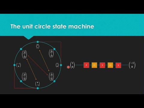
Quantum computation is formulated through linear algebra, modeling qubits as normalized two-dimensional state vectors whose superpositions can be transformed using reversible unitary gates. (4:23)
The Deutsch oracle problem provides the foundational proof of quantum speedup, evaluating whether a black-box function is constant or variable in a single query compared to two queries classically. (33:09)
Quantum entanglement permits instantaneous non-local coordination faster than light, while Bell's theorem and causality ensure that faster-than-light communication remains strictly impossible. (61:45)
Practical fault tolerance demands significant hardware redundancy, requiring an estimated 100 to 200 physical qubits to construct a single reliable, error-corrected logical qubit. (74:45)
Detailed notes
## Background
Published on YouTube by Microsoft Research on May 14, 2018, this technical lecture strips away hand-wavy pop-science analogies to explain quantum computing through a computer science framework. The presentation walks through linear algebra foundations, qubit mechanics, and quantum logic gates, culminating in algorithmic solutions like the Deutsch oracle problem and live software and hardware demonstrations in Q# and IBM Quantum.
## TL;DR
The lecture builds a rigorous foundation for quantum computation using state machines, basis vectors, and unitary reversible matrices rather than esoteric physics metaphors. After establishing how qubits, superposition, and quantum gates function mathematically, the speaker details how the Deutsch oracle problem achieves quantum speedup via phase kickback and interference in a single query. The talk extends into multi-qubit entanglement, Bell's theorem, and the mechanics of quantum teleportation while explaining error-correction scaling bottlenecks. It concludes with an end-to-end demonstration running the Deutsch algorithm in Q# alongside empirical measurement data from a physical IBM dilution refrigerator processor.
## Atmosphere & style
The presentation carries an energetic, demystifying, and intellectually grounded tone, blending dry humor with crisp linear algebra on the whiteboard. By treating quantum strangeness as straightforward matrix operations rather than mystical pop-science phenomena, the speaker fosters an engaging, accessible classroom dynamic. Watching it feels like a refreshing conceptual breakthrough, turning what is often perceived as an impenetrable physics topic into an intuitive and solvable programming model.
## Bulletin
- [04:23](https://www.youtube.com/watch?v=F_Riqjdh2oM&t=263s) Quantum computation is formulated through linear algebra, modeling qubits as normalized two-dimensional state vectors whose superpositions can be transformed using reversible unitary gates.
- [33:09](https://www.youtube.com/watch?v=F_Riqjdh2oM&t=1989s) The Deutsch oracle problem provides the foundational proof of quantum speedup, evaluating whether a black-box function is constant or variable in a single query compared to two queries classically.
- [01:01:45](https://www.youtube.com/watch?v=F_Riqjdh2oM&t=3705s) Quantum entanglement permits instantaneous non-local coordination faster than light, while Bell's theorem and causality ensure that faster-than-light communication remains strictly impossible.
- [01:14:45](https://www.youtube.com/watch?v=F_Riqjdh2oM&t=4485s) Practical fault tolerance demands significant hardware redundancy, requiring an estimated 100 to 200 physical qubits to construct a single reliable, error-corrected logical qubit.
## Key takeaways
- [00:04](https://www.youtube.com/watch?v=F_Riqjdh2oM&t=4s) Quantum computing can be completely understood through computer science abstractions and linear algebra, avoiding hand-wavy physical metaphors.
- [04:23](https://www.youtube.com/watch?v=F_Riqjdh2oM&t=263s) Classical bits map to two-dimensional orthogonal basis vectors |0⟩ and |1⟩, with operations represented as matrix multiplications.
- [09:38](https://www.youtube.com/watch?v=F_Riqjdh2oM&t=578s) Quantum computation relies strictly on reversible operations, which bypass the thermodynamic energy dissipation defined by the Landauer limit.
- [10:43](https://www.youtube.com/watch?v=F_Riqjdh2oM&t=643s) Combining multi-bit or multi-qubit systems via tensor products creates an exponential state space of dimension 2^n.
- [16:33](https://www.youtube.com/watch?v=F_Riqjdh2oM&t=993s) A qubit exists in a genuine simultaneous superposition of states with complex amplitudes until measurement forces an irreversible probabilistic collapse.
- [27:23](https://www.youtube.com/watch?v=F_Riqjdh2oM&t=1643s) The Hadamard gate acts as its own inverse, enabling quantum algorithms to enter superposition and deterministically exit it without destructive intermediate measurement.
- [33:09](https://www.youtube.com/watch?v=F_Riqjdh2oM&t=1989s) The Deutsch oracle demonstrates quantum advantage by classifying a function as constant or balanced in one query using phase kickback on an ancilla qubit.
- [53:23](https://www.youtube.com/watch?v=F_Riqjdh2oM&t=3203s) The progression from Deutsch's algorithm to the Deutsch-Jozsa and Simon's algorithms directly enabled Shor's algorithm for exponential integer factorization.
- [57:57](https://www.youtube.com/watch?v=F_Riqjdh2oM&t=3477s) Quantum entanglement represents composite states that mathematically cannot be decomposed into tensor products of individual qubit states.
- [01:01:45](https://www.youtube.com/watch?v=F_Riqjdh2oM&t=3705s) Entanglement enables faster-than-light state coordination, but Bell's theorem and the impossibility of forced local outcomes prevent faster-than-light communication.
- [01:08:26](https://www.youtube.com/watch?v=F_Riqjdh2oM&t=4106s) The no-cloning theorem dictates that unknown quantum states cannot be duplicated, allowing quantum teleportation only as a destructive state transfer requiring two classical bits.
- [01:14:45](https://www.youtube.com/watch?v=F_Riqjdh2oM&t=4485s) Simulating quantum systems on classical computers requires exponential memory scaling as 2^N complex amplitudes across the entangled state space.
- [01:16:30](https://www.youtube.com/watch?v=F_Riqjdh2oM&t=4590s) Skeptics like mathematician Gil Kalai argue that exponential scaling of hardware noise and decoherence might fundamentally prevent scalable quantum computation.
- [01:27:06](https://www.youtube.com/watch?v=F_Riqjdh2oM&t=5226s) Live execution of Bell state circuits on physical IBM hardware demonstrates real entanglement alongside residual noise from thermal effects and gate infidelity.
## Detailed walkthrough
### [00:04](https://www.youtube.com/watch?v=F_Riqjdh2oM&t=4s) Introduction: A Computer Science Perspective on Quantum Mechanics
The speaker welcomes attendees to the talk, playfully noting that it falls on Valentine's Day: “Happy Valentine's Day. We will learn about this most romantic of all subjects, Quantum Computing.” The session is explicitly designed for computer scientists rather than physicists. The speaker clarifies right at the outset that there will be virtually no physics covered—no discussions of the Double-Slit Experiment or Heisenberg's Uncertainty Principle.
Instead, the session frames quantum computing around a familiar computer science abstraction: a state machine. The plan for the session is to introduce this computational model, run a quantum algorithm demonstrating how it surpasses classical computation, and conclude with practical demonstrations, including a program running in Q#, Microsoft's quantum programming language. The focus is specifically on the gate quantum computation model, where bits are routed through logic gates that apply transformations, directly paralleling classical digital logic. The speaker contrasts this with the quantum annealing model utilized by D-Wave, pointing out that while some speculate annealing and gate-based quantum computing might be computationally equivalent, that question remains open, and the rest of the presentation will concentrate strictly on gate-based models.
[01:11](https://www.youtube.com/watch?v=F_Riqjdh2oM&t=71s) Motivations: Supremacy, Impactful Algorithms, and Intellect
To motivate why computer scientists should invest time into quantum computing, the speaker lays out three core drivers:
```mermaid
flowchart TD
accTitle: Motivations for Learning Quantum Computing
accDescr: Three primary drivers motivating quantum computing research: commercial viability, practical algorithms, and intellectual curiosity.
subgraph M2["2. Powerful Algorithmic Applications"]
C["Shor's Algorithm: Factor RSA"]
D["Grover's: Search Unordered List in O(√N)"]
E["Simulating Quantum Systems: Drug Design & N-Fixation"]
end
subgraph M3["3. Intellectual Curiosity"]
F["Defies Classical Mental Models"]
G["Requires Math Instead of Flawed Analogies"]
end
M1 --> M2 --> M3
```
1. **Quantum Supremacy and Industry Momentum:** Quantum supremacy—running a real-world task on a physical quantum computer faster in real time than on any classical computer—is anticipated within the very year of the talk (2018), with Google announcing ambitions to demonstrate it. Major industry players like Microsoft, Google, Intel, and IBM are actively pouring billions of dollars into development.
2. **Transformative Algorithmic Applications:**
- *Shor's Algorithm:* The landmark discovery that put quantum computing on the economic map by showing RSA encryption can be efficiently factored, carrying profound implications for global financial systems.
- *Unordered Database Search:* While classical search over an unsorted collection of $N$ items fundamentally requires checking each element in $O(N)$ operations, a quantum search can locate the item in $O(\sqrt{N})$ queries.
- *Quantum Simulation:* Regarded by the speaker as having the greatest likelihood of changing everyday human life, quantum machines offer exponential speedups in modeling quantum-mechanical interactions. This has massive ramifications for molecular biology, drug discovery, and catalyst design—specifically nitrogen fixation, a hallmark application in Microsoft's quantum research narrative.
3. **Intellectual Challenge and Linguistic Limits:** The speaker's personal motivation stems from pure intellectual fascination. Seasoned engineers can look at almost any classical software or mechanical apparatus and construct a rough mental model of how it operates. Quantum computers, however, thoroughly defy that intuition: “Like how can a quantum computer outperform classical computation? It doesn't make any sense.” The speaker argues philosophically that human everyday language evolved entirely inside a classical realm and simply lacks the descriptive vocabulary for quantum behavior. Consequently, popular-science metaphors inevitably ring hollow. The only medium that accurately describes the quantum domain without deception is mathematics, citing theoretical physicist David Mermin's famous quip: “Shut up and calculate.”
[04:23](https://www.youtube.com/watch?v=F_Riqjdh2oM&t=263s) Agenda and Representing Bits as Linear Algebra
The talk maps out a clean four-stage curriculum:
1. Representing basic classical computation through linear algebra (vectors, matrices, matrix multiplication).
2. Generalizing those linear algebraic tools to understand qubits, superpositions, and quantum logic gates.
3. Tackling the Deutsch oracle problem—the simplest concrete scenario where a quantum algorithm demonstrably beats classical logic.
4. Exploring bonus phenomena—quantum entanglement and quantum teleportation—followed by live code demos in Q#.
The speaker begins the linear algebra foundation by mapping binary bit states to standard two-dimensional basis column vectors:
- A classical state of $0$ is mapped to $\begin{bmatrix} 1 \\ 0 \end{bmatrix}$.
- A classical state of $1$ is mapped to $\begin{bmatrix} 0 \\ 1 \end{bmatrix}$.
These are also expressed using Dirac vector notation (ket notation) as $|0\rangle$ and $|1\rangle$. A simple conceptual trick for remembering this encoding is to view the vector as a zero-indexed array: having a value of $1$ at index position 0 denotes the state 0, whereas having a value of $1$ at index position 1 represents the state 1.
[05:51](https://www.youtube.com/watch?v=F_Riqjdh2oM&t=351s) Matrix Multiplication Review and Single-Bit Operations
The speaker runs through a rapid review of matrix-vector multiplication. When multiplying a $2 \times 2$ matrix by a $2 \times 1$ column vector:
$$\begin{bmatrix} a & b \\ c & d \end{bmatrix} \begin{bmatrix} x \\ y \end{bmatrix} = \begin{bmatrix} ax + by \\ cx + dy \end{bmatrix}$$
The same principle extends naturally to higher dimensions (such as $3 \times 3$ matrices acting on three-element vectors). The identity matrix $I$ (often designated simply as $\mathbf{1}$) contains ones exclusively along the main diagonal and zeros everywhere else, acting as a multiplicative identity ($I \mathbf{v} = \mathbf{v}$). The speaker shares a helpful mental shortcut for permutation-style matrices often seen in quantum circuits: if a matrix resembles the identity but has its middle two rows swapped, multiplying a vector by that matrix directly swaps the middle two elements of the resulting vector.
Turning to computation, the speaker quizzes the audience on the total number of single-bit operations. While attendees initially volunteer multi-bit logic gates like AND, OR, and XOR, the audience quickly identifies the four single-input, single-output Boolean functions on a single bit:
- **Identity ($f(x) = x$):** Leaves the bit unchanged; mapped to the $2 \times 2$ identity matrix $\begin{bmatrix} 1 & 0 \\ 0 & 1 \end{bmatrix}$.
- **Negation ($f(x) = \text{NOT } x$):** Inverts the bit; mapped to $\begin{bmatrix} 0 & 1 \\ 1 & 0 \end{bmatrix}$.
- **Constant-0 ($f(x) = 0$):** Forces the output to 0 regardless of input; mapped to $\begin{bmatrix} 1 & 1 \\ 0 & 0 \end{bmatrix}$.
- **Constant-1 ($f(x) = 1$):** Forces the output to 1 regardless of input; mapped to $\begin{bmatrix} 0 & 0 \\ 1 & 1 \end{bmatrix}$.
Multiplying these matrices by the $|0\rangle$ and $|1\rangle$ basis vectors directly yields the expected bit outcomes.
The speaker connects these single-bit matrices to the concept of reversible computing—a concept popularized in science fiction works such as Charles Stross's novel *Accelerando*. A computational operation is strictly reversible if knowledge of the operation and its resulting output allows one to unambiguously deduce the original input.
- **Permutations are Reversible:** Operations that merely reorder or flip states preserve state information. Both the Identity gate and the Negation (NOT) gate are fully reversible: if an output of $1$ emerges from a NOT gate, the input is guaranteed to have been $0$.
- **Erasing is Irreversible:** Operations that overwrite states destroy information. Constant-0 and Constant-1 are non-reversible; if a Constant-1 gate outputs a $1$, it is impossible to determine whether the original input was a $0$ or a $1$. In the speaker's words: “It's not reversible. It erases information.”
[09:38](https://www.youtube.com/watch?v=F_Riqjdh2oM&t=578s) Reversible Computing and the Landauer Limit
The speaker explains that quantum computers rely exclusively on reversible operations. Out of the classical operations previously introduced, the only ones relevant to quantum computing are negation (the NOT gate) and the identity operation, though the speaker jokes that identity is merely “the same as doing nothing.” A further rule of quantum computers is that their operations are self-inverting: applying the exact same operation twice restores the original input state.
Venturing briefly into a “pop science” aside, the speaker brings up the Landauer limit (colloquially mentioned alongside von Neumann), which physicists calculate as the theoretical minimum amount of energy required to perform an irreversible computational step, such as erasing a bit. Reversible computing offers the tantalizing theoretical possibility of bypassing that thermodynamic dissipation barrier entirely. While modern processors consume millions of times more energy than this theoretical threshold, the speaker quips, “Now, currently, processors needs millions of times more energy than the Von Neumann [Landauer] Limit but, you know, 5,000 years from now, who knows? Pretty nifty.”
- Quantum computers strictly evaluate operations that are reversible and self-inverting ($A \cdot A = I$).
- Non-reversible operations inherently dissipate energy according to fundamental thermodynamic physical limits.
- Modern hardware operates far above this theoretical limit, but reversible paradigms present a path toward unprecedented energy efficiency.
---
[10:43](https://www.youtube.com/watch?v=F_Riqjdh2oM&t=643s) Multibit Systems and the Tensor Product
To represent multiple bits at once, linear algebra uses the tensor product ($\otimes$), a concept often skipped in introductory classes but straightforward to execute. Taking the tensor product of two vectors involves taking the second vector and tiling copies of it scaled by each individual element of the first vector. For example, if vector $X$ has entries $x_0, x_1$ and vector $Y$ has entries $y_0, y_1$, the resulting vector is $[x_0 y_0, \, x_0 y_1, \, x_1 y_0, \, x_1 y_1]^T$. With numeric vectors like $[1, 2]^T \otimes [3, 4]^T$, this produces $[1 \cdot 3, 1 \cdot 4, 2 \cdot 3, 2 \cdot 4]^T = [3, 4, 6, 8]^T$.
When applied to the standard basis vectors representing classical bits ($0$ as $[1, 0]^T$ and $1$ as $[0, 1]^T$), the resulting product vector always contains a single $1$ and all other entries as $0$. The single non-zero entry corresponds to the decimal index of the binary state:
- $|00\rangle = [1, 0]^T \otimes [1, 0]^T = [1, 0, 0, 0]^T$ (index 0)
- $|01\rangle = [1, 0]^T \otimes [0, 1]^T = [0, 1, 0, 0]^T$ (index 1)
- $|10\rangle = [0, 1]^T \otimes [1, 0]^T = [0, 0, 1, 0]^T$ (index 2)
- $|11\rangle = [0, 1]^T \otimes [0, 1]^T = [0, 0, 0, 1]^T$ (index 3)
Tensing three bits together yields an 8-element vector (for instance, $|100\rangle$, representing decimal 4, places a $1$ at index 4). The speaker promises not to tensor three bits together frequently because these vectors grow exponentially: an $n$-bit state requires a vector of dimension $2^n$. The speaker emphasizes: “Here, we see a sort of whisper of the power of quantum computing in this exponential term but hold that thought, we'll get back to it.”
```mermaid
flowchart TD
accTitle: Two-Bit State Representation via Tensor Product
accDescr: Diagram illustrating how two single-bit vectors combine via a tensor product into a four-dimensional product state vector.
subgraph Operation["Kronecker / Tensor Product"]
TP["Tensor Product (⊗)"]
end
subgraph ProductState["Combined 2ⁿ State Vector"]
Out["[x0·y0, x0·y1, x1·y0, x1·y1]ᵀ<br/>Dimension: 2² = 4"]
end
A --> TP
B --> TP
TP --> Out
```
---
[13:06](https://www.youtube.com/watch?v=F_Riqjdh2oM&t=786s) The CNOT Gate as the Building Block of Reversible Logic
The speaker introduces the Controlled-NOT (CNOT) gate, a fundamental operation in both reversible and quantum computing. Operating on a pair of bits, CNOT designates one as the control bit and the other as the target bit. If the control bit is $1$, the target bit is inverted; if the control bit is $0$, the target bit remains untouched. The control bit is never altered. Setting the most significant bit as the control and the least significant bit as the target yields the mappings:
- $00 \rightarrow 00$
- $01 \rightarrow 01$
- $10 \rightarrow 11$
- $11 \rightarrow 10$
Walking step-by-step through the matrix multiplication, the speaker applies this matrix to the product states for $10$ and $11$, demonstrating that multiplying the vector by the matrix precisely replicates the expected bit-flip behavior. An audience member asks whether factoring combined product states back into individual bit vectors is always possible or practical for larger vectors. The speaker answers that it is practical, but adds, “Not always possible, which we'll get into that when we get into quantum entanglement, basically, but good question.”
The speaker draws an analogy between classical CPUs and reversible circuits: while classical computing builds everything out of NAND gates, CNOT serves as the analogous core building block for reversible systems. However, CNOT alone is not universal; constructing every conceivable reversible logical function requires an additional primitive such as the three-bit Toffoli gate, though the speaker notes that the Toffoli gate will not be needed for this presentation.
---
[16:33](https://www.youtube.com/watch?v=F_Riqjdh2oM&t=993s) Transition to Qubits, Superposition, and Measurement
Summarizing the classical linear algebra framework, the speaker recaps that bits are two-dimensional basis vectors ($[1, 0]^T$ and $[0, 1]^T$), gates are matrices, multi-bit systems are formed via tensor products, and CNOT acts as a primary building block. With this foundation in place, the speaker transitions to quantum computing with a reveal: classical bits (cbits) have been qubits all along, merely restricted to special cases.
A qubit is defined generally as a two-element column vector $[a, b]^T$, where $a$ and $b$ are complex numbers, though for this lecture the speaker keeps things accessible by restricting them entirely to real numbers. The state must satisfy the normalization constraint:
$$a^2 + b^2 = 1$$
Under this rule, classical states $[1, 0]^T$ and $[0, 1]^T$ naturally fit because $1^2 + 0^2 = 1$. The speaker walks through other valid qubit states:
- $\left[\frac{1}{\sqrt{2}}, \frac{1}{\sqrt{2}}\right]^T$, because $\left(\frac{1}{\sqrt{2}}\right)^2 + \left(\frac{1}{\sqrt{2}}\right)^2 = \frac{1}{2} + \frac{1}{2} = 1$.
- $\left[\frac{1}{2}, \frac{\sqrt{3}}{2}\right]^T$, because $\left(\frac{1}{2}\right)^2 + \left(\frac{\sqrt{3}}{2}\right)^2 = \frac{1}{4} + \frac{3}{4} = 1$.
- Negative values such as $[-1, 0]^T$ or $\left[\frac{1}{\sqrt{2}}, -\frac{1}{\sqrt{2}}\right]^T$, because squaring a negative yields a positive number.
When a qubit is not purely $[1, 0]^T$ or $[0, 1]^T$, it is in a *superposition* of both states simultaneously—the technical underpinning of popular metaphors like Schrödinger’s cat being alive and dead. Being in superposition allows a system to “kind of compute with the values of both zero and one at the same time,” hinting once again at quantum speedup.
To retrieve data from a quantum computation, the qubit must pass through a measurement gate, causing its superposition to collapse probabilistically into standard classical states:
- The state collapses to $0$ with probability $a^2$.
- The state collapses to $1$ with probability $b^2$.
For the state $\left[\frac{1}{\sqrt{2}}, \frac{1}{\sqrt{2}}\right]^T$, measurement results in a 50% chance of collapsing to $0$ and a 50% chance of collapsing to $1$, behaving like an ideal fair coin-flip. In contrast, measuring a classical bit like $[1, 0]^T$ has a 100% probability ($1^2 = 1$) of collapsing to $0$.
[20:01](https://www.youtube.com/watch?v=F_Riqjdh2oM&t=1201s) Physical Intuition: Polarization and Qubit Measurement
The speaker wraps up the discussion of single-qubit measurement probabilities by noting that a state like $[0, 1]^T$ has a 100 percent chance of collapsing into $1$, making measurement idempotent. To ground these mathematical vectors in reality, the speaker offers an everyday physical analogy: polarized sunglasses. Light polarization is fundamentally a quantum phenomenon where photons oscillate in specific orientations, such as horizontal or vertical. Polarized lenses are manufactured with microscopic gratings oriented along a single axis, allowing only light aligned with that specific angle to pass through while blocking the rest.
In quantum computing terms, a photon polarized along one axis can represent a $0$, while a photon polarized perpendicularly represents a $1$. A qubit in superposition can be thought of as a photon oriented at an intermediate angle, effectively embodying both polarizations at once. When attempting to measure such a photon, an experimenter fires it at a polarizing filter: it either makes it through or is absorbed, collapsing its state definitively into a $0$ or a $1$. The speaker cautions the audience not to take the hardware analogy too far, explaining that while optical polarization provides clean mental scaffolding, practical implementations avoid it: “Of course, modern, we found that photons actually make very, very poor qubits, they tend to collapse too easily.”
- Horizontal and vertical photon polarizations map directly to classical basis states $|0\rangle$ and $|1\rangle$.
- Physical measurement acts like a polarization grating, forcing an ambiguous state to collapse upon observation.
- Free-flying photons are notoriously fragile qubits because ambient physical interactions trigger unwanted decoherence and state collapse.
[21:18](https://www.youtube.com/watch?v=F_Riqjdh2oM&t=1278s) Multiple Qubits and the Tensor Product
Moving from individual qubits to multi-qubit registers, the speaker demonstrates that the mathematical framework mirrors classical bit combinations using the tensor product. When two independent qubits are tensored together, the fundamental identity requiring the sum of squared amplitudes to equal one is strictly maintained. For example, taking two balanced qubits—each representing a 50 percent coin flip with amplitude $1/\sqrt{2}$ for both states—and calculating their tensor product yields a single four-dimensional state vector where every entry is $1/2$. Squaring each component produces $(1/2)^2 = 1/4$, and summing the four components yields $1/4 + 1/4 + 1/4 + 1/4 = 1$.
```mermaid
flowchart LR
accTitle: Two-Qubit Tensor Product and Measurement
accDescr: Diagram showing two superposition qubits combined via tensor product into a four-state vector and collapsing to a single state upon measurement.
subgraph Inputs["Individual Qubits"]
Q0["Qubit 0: [1/√2, 1/√2]"]
Q1["Qubit 1: [1/√2, 1/√2]"]
end
subgraph Product["Tensor State"]
TP["4-Vector: [1/2, 1/2, 1/2, 1/2]ᵀ"]
end
subgraph Measurement["Measurement Outcomes"]
M["Equal 25% collapse chance:
|00⟩, |01⟩, |10⟩, or |11⟩"]
end
Q0 --> TP
Q1 --> TP
TP --> M
```
Reading this four-vector corresponds directly to measurement probabilities: observing the two-qubit system yields an equal 25 percent chance of collapsing into $|00\rangle$, $|01\rangle$, $|10\rangle$, or $|11\rangle$. An attendee asks whether, after measurement, only a single $1$ remains in the resulting state vector or if multiple ones could appear simultaneously. The speaker confirms that measurement leaves exactly one entry set to $1$ and all other entries set to $0$: “There could not be two ones because that would actually violate our $a^2 + b^2 = 1$ constraint.” The collapsed vector can then be factored cleanly back into individual classical bits, establishing a baseline for multi-qubit systems before entangling operations are introduced.
- Tensoring two 50/50 superposition qubits yields a 4-vector with uniform amplitudes of $1/2$.
- Each basis state in a two-qubit system has an amplitude whose square gives the probability of collapsing to that specific two-bit combination.
- Measurement collapses the entire multi-qubit state into a single one-hot basis vector, ensuring total probability never exceeds unity.
[23:27](https://www.youtube.com/watch?v=F_Riqjdh2oM&t=1407s) Quantum Gates and the Hadamard Transformation
Having established how multi-qubit states are formed, the speaker turns to how quantum states are manipulated. Just as in classical computing, operations are implemented via matrix multiplication, and familiar classical gates like negation carry over directly. If an asymmetric qubit with a 25 percent probability of collapsing to $0$ and a 75 percent probability of collapsing to $1$ is passed through a bit-flip operator, the probabilities invert to 75 percent for $0$ and 25 percent for $1$. Physical quantum logic gates act as precision laboratory devices that interact gently with qubits: they exert enough influence to transform probability amplitudes without triggering decoherence or premature collapse.
The most critical operator introduced is the Hadamard gate, which creates equal superpositions from pure classical inputs. The Hadamard matrix consists of $1/\sqrt{2}$ in every entry, save for the bottom-right corner, which holds $-1/\sqrt{2}$. Applying the Hadamard gate to $|0\rangle$ yields $[1/\sqrt{2}, 1/\sqrt{2}]^T$, while applying it to $|1\rangle$ yields $[1/\sqrt{2}, -1/\sqrt{2}]^T$. When the speaker quizzes the room on why the bottom-right element must be negative, an attendee hesitates over matrix dimensions. The speaker clarifies the underlying requirement: “Well, the answer basically has to be reversible.” Without the negative sign, inputs of both $0$ and $1$ would produce identical output vectors, destroying reversibility and violating the unitary laws of quantum mechanics.
- The Hadamard matrix is defined as $\frac{1}{\sqrt{2}} \begin{bmatrix} 1 & 1 \\ 1 & -1 \end{bmatrix}$.
- Applying Hadamard to $|0\rangle$ produces $[1/\sqrt{2}, 1/\sqrt{2}]^T$; applying it to $|1\rangle$ produces $[1/\sqrt{2}, -1/\sqrt{2}]^T$.
- The negative entry in the matrix is mandatory to keep the operation reversible and avoid mapping different inputs to identical outputs.
[25:39](https://www.youtube.com/watch?v=F_Riqjdh2oM&t=1539s) The Nature of Superposition and Quantum Phase
An attendee asks for clarification regarding what superposition truly means, prompting the speaker to confront a widespread misconception. Superposition does not mean a qubit possesses a secret, pre-existing value of $0$ or $1$ that observers simply have not uncovered yet. Instead, the particle genuinely exists in both states at the same time until an external observation forces a collapse: “This doesn't mean the qubit is secretly zero or secretly one, and we don't know; it means it's actually in both at the same time, this is just quantum weirdness.” At subatomic scales, physical systems do not possess definite, classical properties until they interact with a measurement apparatus.
This leads another audience member to ask why the Hadamard gate produces two seemingly different superposition states—one with a positive lower component and one with a negative lower component—if both represent a 50/50 probability of collapsing to $0$ or $1$. The speaker emphasizes the critical distinction between classical observation and the internal quantum realm. From a classical observer's viewpoint after measurement, both states appear identical because squaring either $1/\sqrt{2}$ or $-1/\sqrt{2}$ yields an identical 50 percent probability. However, inside the unobserved quantum computer, the minus sign represents a distinct phase difference:
> “Has a sense that it used to be one? Not really, it just ends up in this state, which is different within the quantum realm than this state. These are two different states... Both when you measure it and convert it into the classical world come down with a 50-50 chance. Yes. But they are different, and they have different computational properties.”
- Superposition is not classical ignorance or hidden variables; the qubit objectively occupies both states simultaneously.
- Amplitudes of $1/\sqrt{2}$ and $-1/\sqrt{2}$ result in identical measurement probabilities of 50 percent when squared.
- The negative amplitude stores quantum phase information that persists and drives interference effects as long as no measurement takes place.
[27:23](https://www.youtube.com/watch?v=F_Riqjdh2oM&t=1643s) Leaving Superposition Without Measurement and Algorithm Structure
The speaker reveals a surprising mathematical property of the Hadamard gate: it is its own inverse ($H = H^\dagger = H^{-1}$). Multiplying the Hadamard matrix by the positive superposition state $[1/\sqrt{2}, 1/\sqrt{2}]^T$ transforms it directly back into a classical $0$, while multiplying it by $[1/\sqrt{2}, -1/\sqrt{2}]^T$ yields a classical $1$. This provides a mechanism for transitioning out of superposition back into definitive classical values without relying on destructive, probabilistic measurement.
```mermaid
flowchart LR
accTitle: Canonical Quantum Algorithm Architecture
accDescr: Pipeline showing classical bits converted to superposition, processed with quantum operators, and transformed back to deterministic classical bits.
CIn["Classical Bits: |0⟩, |1⟩"] --> HIn["Hadamard Gates (Create Superposition)"]
HIn --> QOps["Quantum Processing (Interference & Phase Shifts)"]
QOps --> HOut["Hadamard / Unitary Unrolling"]
HOut --> COut["Deterministic Classical Output"]
```
This self-inverting property establishes the canonical architecture of quantum algorithms. A computation begins with well-defined classical bits, uses Hadamard gates to inject them into superposition, performs phase manipulations and quantum interference across the state space, and finally collapses the states back down using complementary gates: “We can start with our classical bit values, we put them into superposition, do a bunch of quantum stuff to them, and at the end if we're clever, we can transition them to zero or one so that our whole computation was deterministic.” The speaker notes that while some algorithms, such as Shor's algorithm, are inherently probabilistic and only succeed around 50 percent of the time per run, other algorithms achieve fully deterministic results. When an attendee asks how basic arithmetic like $2 + 2$ is structured, the speaker clarifies that while any classical computation can run on a quantum system by restricting values to classical zeros and ones, standard addition achieves no quantum speedup and is a waste of quantum hardware.
- The Hadamard operation is self-inverting: applying it twice sequentially returns the system to its original classical basis state.
- Structured interference allows quantum algorithms to output deterministic answers rather than random measurement samples.
- Classical algorithms can execute natively on quantum computers, but quantum advantage only emerges on problems suited to interference and superposition.
[29:18](https://www.youtube.com/watch?v=F_Riqjdh2oM&t=1758s) The Unit Circle State Machine
To help software engineers and computer scientists build an intuitive model of qubit operations, the speaker maps single-qubit states onto the familiar unit circle ($x^2 + y^2 = 1$) from high school trigonometry. In this geometric mapping, the top entry of a state vector corresponds to the x-coordinate, while the bottom entry corresponds to the y-coordinate. The classical basis state $|0\rangle$, represented by vector $[1, 0]^T$, sits on the horizontal X-axis at position $(1, 0)$. The classical basis state $|1\rangle$, represented by $[0, 1]^T$, sits on the vertical Y-axis at position $(0, 1)$.
“And this is the bit flip operator, it defines transitions around this unit circle.” Passing states through the bit-flip matrix causes geometric reflections across the axes: $[1, 0]^T$ flips to $[0, 1]^T$, and $[0, -1]^T$ flips to $[-1, 0]^T$. However, when the bit-flip operator is applied to the diagonal superposition states, its behavior shifts. For the symmetric state $[1/\sqrt{2}, 1/\sqrt{2}]^T$, swapping coordinates leaves the vector unchanged. For states with opposing signs, such as $[1/\sqrt{2}, -1/\sqrt{2}]^T$, the operator drives a transition directly across the unit circle, a geometric shift that quantum algorithms leverage to execute selective phase inversions.
- The unit circle provides a geometric state-machine visualization where $|0\rangle = (1, 0)$ and $|1\rangle = (0, 1)$.
- The bit-flip (Pauli-X) operator rotates and reflects coordinates along the unit circle, exchanging classical basis states.
- Balanced superposition vectors lie along diagonal axes, where bit flips either leave the state invariant or reflect it across the origin.
[30:33](https://www.youtube.com/watch?v=F_Riqjdh2oM&t=1833s) Visualizing Gates on the Unit Circle and Quantum Circuits
The geometric representation of single-qubit operations provides an intuitive state machine model without requiring continuous matrix multiplication. The bit-flip operator ($X$) and the Hadamard gate ($H$) act as transitions across the unit circle. While real numbers restrict the geometry to a circle, moving to complex numbers expands this structure into the three-dimensional Bloch sphere. Using the circle model, a sequence of gates can be traced visually: starting at state $\begin{bmatrix}1 \\ 0\end{bmatrix}$ (state $|0\rangle$), applying an $X$ gate flips it to $\begin{bmatrix}0 \\ 1\end{bmatrix}$ ($|1\rangle$), followed by a Hadamard gate into superposition $\begin{bmatrix}1/\sqrt{2} \\ -1/\sqrt{2}\end{bmatrix}$, then another $X$ gate, another Hadamard, and a final $X$ gate, stepping around the circle to return to a basis state.
```mermaid
flowchart LR
accTitle: Single Qubit Gate Sequence
accDescr: Sequence of bit flip and Hadamard gates operating reversibly on a qubit state.
subgraph Circuit["Quantum Circuit Traversal"]
direction LR
qIn["|0>"] --> X1["X"]
X1 --> H1["H"]
H1 --> X2["X"]
X2 --> H2["H"]
H2 --> X3["X"]
X3 --> qOut["|1>"]
end
```
The speaker notes that these operations are entirely reversible, meaning reversing the gate sequence traces the exact path backward: “It's nice to know that additional dimension is always available to us if we want to make our computation even more powerful.” This state-machine perspective grounds the core rules established so far: classical bits are special cases of qubits; qubits are normalized 2-vectors satisfying $a^2 + b^2 = 1$; measurement probabilistically collapses superpositions; multi-qubit systems are formed via tensor products; and operations are unitary matrices that preserve vector lengths.
- Real amplitudes restrict quantum state vectors to the perimeter of the 2D unit circle.
- Full complex amplitudes generalize the unit circle to the Bloch sphere.
- Quantum circuit notation depicts qubits flowing left to right along horizontal wires while passing through gate blocks.
---
[33:09](https://www.youtube.com/watch?v=F_Riqjdh2oM&t=1989s) The Deutsch Oracle: Identifying Functions vs. Determining Function Types
To demonstrate where quantum computers gain an advantage over classical hardware, the speaker introduces the Deutsch oracle problem, first proposed by David Deutsch around 1983. In this setup, a user is handed a black box implementing an unknown function on a single bit. There are four possible single-bit functions: constant zero (`set zero`), constant one (`set one`), identity, and bit flip (`negation`). To determine exactly which of the four functions is hidden inside, a classical machine must test both $0$ and $1$, requiring two queries. When the speaker asks how many queries a quantum computer needs to pinpoint the exact function, the audience guesses one, but the speaker corrects them: it still takes two queries.
The speaker emphasizes this limitation to dispel a widespread myth: “I say this to illustrate an important point, which is quantum computers, they don't really compute with all values simultaneously.” Because any readout collapses the qubit into a single classical bit, one bit of measurement cannot supply the two bits of entropy needed to differentiate among four possibilities. However, the problem changes if the goal is only to classify whether the function is **constant** (constant zero, constant one) or **variable** (identity, bit flip). Classically, one query still yields ambiguous results—evaluating $f(0) = 0$ could mean the function is either constant zero or identity, necessitating a second evaluation of $f(1)$. A quantum computer, by contrast, can exploit superposition to determine whether the function is constant or variable in a single query.
---
[35:42](https://www.youtube.com/watch?v=F_Riqjdh2oM&t=2142s) Rewiring Black Boxes for Reversible Quantum Evaluation
Implementing arbitrary single-bit functions on a quantum computer immediately runs into the constraint of reversibility. Constant functions map both inputs ($0$ and $1$) to the same output, discarding information and violating the requirement that quantum operators be unitary and invertible: “They're not reversible, how are we going to write these non-reversible functions on a reversible computer?”
```mermaid
flowchart LR
accTitle: Reversible Oracle Black Box
accDescr: Quantum black box with input wire passing through unchanged and output wire receiving f(x).
subgraph Oracle["Reversible Oracle Black Box"]
direction LR
inX["|x> (Input)"] --> passX["|x> (Unchanged)"]
inY["|0> (Ancilla)"] --> outY["|f(x)> (Result)"]
end
```
To resolve this, quantum algorithms use a standard construction: adding an extra ancilla qubit wire. Instead of a single wire passing through the black box, two wires are used:
1. **Input wire ($x$):** Carries the input state through the transformation completely unchanged, preserving the history so the operation remains mathematically reversible.
2. **Output wire ($y$):** Initialized to state $|0\rangle$, this wire is modified inside the box so that the function value $f(x)$ is written directly onto it.
An audience member expresses confusion about why the output wire must be initialized to $|0\rangle$ and fed in simultaneously if it is labeled an output. The speaker clarifies that in quantum circuit diagrams, all participating qubits span the full duration of the circuit; the circuit assumes the helper wire arrives as $|0\rangle$ so the internal gates can reliably write $f(x)$ to it. Another audience member asks whether multiple boxes could be chained in series by feeding the $f(x)$ output into the input of a subsequent stage, prompting the speaker to acknowledge that cascading stages in series is another valid structural approach.
[40:19](https://www.youtube.com/watch?v=F_Riqjdh2oM&t=2419s) Constructing a Reversible Two-Qubit Black Box
The discussion begins with an audience member attempting to conceptualize how the black box works across multiple stages—specifically whether the upper-right output $f(x)$ feeds directly into the next stage as input. The speaker confirms that while the standard convention assumes the black box receives zero on the auxiliary wire, that assumption can be intentionally broken: “So, the working of black box assumes that the output input is zero, but we can break that assumption and be tricky.” By feeding an alternate value into that wire, one can extract extra information from the system, which forms the exact crux of the quantum speedup they are building toward.
The speaker acknowledges that this material represents a major intellectual hurdle: “I swear, this is the most difficult part conceptually of this entire presentation.” Rather than rushing past the abstraction, the speaker offers to walk through each of the four possible single-bit functions ($f(x) = 0$, $f(x) = 1$, identity $f(x) = x$, and negation $f(x) = \neg x$) one by one. For constant zero, $x$ enters and leaves on the lower wire unchanged, while the upper-right output wire must always yield zero. Assuming zero enters on the upper wire, the resulting circuit requires no gates whatsoever—it is simply two straight, uninterrupted wires. For constant one, assuming a zero input on the auxiliary line, the output must always be one, which is implemented simply by placing an $X$ (bit-flip) gate on the upper wire.
When an audience member asks whether the two wires could be more intuitively labeled as “computations and its spare” rather than “output” and “input,” the speaker agrees that alternative naming like compute bit and spare bit can help alleviate confusion about having an input wire that doubles as an output wire.
```mermaid
flowchart LR
accTitle: Two-Qubit Oracle Function Encodings
accDescr: Circuit wiring showing how the four single-bit functions are represented reversibly with an input wire and a spare output wire.
subgraph Const0["Constant 0"]
direction LR
c0_in["|0> (spare)"] --> c0_out["|0>"]
c0_x["|x> (input)"] --> c0_xout["|x>"]
end
subgraph Const1["Constant 1"]
direction LR
c1_in["|0> (spare)"] --> c1_x["[ X ]"] --> c1_out["|1>"]
c1_x_in["|x> (input)"] --> c1_xout["|x>"]
end
subgraph Ident["Identity f(x)=x"]
direction LR
id_in["|0> (spare)"] --> id_t["Target (+)"] --> id_out["|x>"]
id_x["|x> (input)"] --> id_c["Control (•)"] --> id_xout["|x>"]
end
subgraph Neg["Negation f(x)=NOT x"]
direction LR
ng_in["|0> (spare)"] --> ng_t["Target (+)"] --> ng_x["[ X ]"] --> ng_out["|NOT x>"]
ng_x["|x> (input)"] --> ng_c["Control (•)"] --> ng_xout["|x>"]
end
```
[43:21](https://www.youtube.com/watch?v=F_Riqjdh2oM&t=2601s) Reversibility, Physical Constraints, and Balanced Functions
An audience member prompts a deeper question: why do we need this two-wire architecture to perform reversible computation in the first place? The speaker contrasts this setup with an ordinary one-wire gate that attempts to map any incoming state unconditionally to zero. Such an operation would correspond to a non-invertible matrix containing rows of ones and zeros, which is mathematically invalid in quantum computing. The speaker stresses that this constraint is not an arbitrary rule of linear algebra: “All this math and stuff I'm showing you, it's not like special it's just, we found that it corresponds to the semantics and workings of a quantum system, and so it's a nice way to reason about it basically.” Because nature prohibits non-unitary, irreversible physical processes, an extra wire is mandatory to preserve information and keep the matrix unitary.
With a two-qubit model, every black box transforms into a four-by-four reversible matrix operating on a product state. The speaker moves to the balanced functions, starting with the identity function, $f(x) = x$. To implement identity, the circuit uses a Controlled-NOT (CNOT) gate where the input wire serves as the control and the spare output wire serves as the target. If a $0$ enters on the input, the target remains unchanged at $0$; if a $1$ enters, the control activates, flipping the target wire to $1$.
To implement negation, $f(x) = \neg x$, an audience member suggests hard-setting the control bit or applying two controlled-NOTs. The speaker clarifies the simpler design: one starts with the identity circuit (a CNOT gate) and follows it with a standard $X$ gate on the output wire. Flipping the resulting bit yields $\neg x$. With all four functions cleanly represented by reversible operations, the foundation for the quantum oracle is complete.
- A single-wire operator mapping all inputs to zero requires a non-reversible matrix such as $\begin{bmatrix}1 & 1 \\ 0 & 0\end{bmatrix}$, which cannot physically exist as a quantum gate.
- The two-qubit architecture ensures every operation can be represented by a valid $4 \times 4$ unitary matrix.
- **Identity function ($f(x) = x$):** Input controls the output via a CNOT gate.
- **Negation function ($f(x) = \neg x$):** CNOT gate followed by an $X$ gate on the output line.
[47:08](https://www.youtube.com/watch?v=F_Riqjdh2oM&t=2828s) The Deutsch Algorithm Workflow and Constant Functions
Having mapped out all four functions, the speaker unveils the full quantum circuit that solves the Deutsch oracle problem in a single query. Rather than supplying $|0\rangle$ to the auxiliary line, the algorithm breaks the default convention. Both the input and output qubits are initialized to $|0\rangle$, then flipped to $|1\rangle$ using $X$ gates. Next, both qubits pass through Hadamard ($H$) gates, placing them into an equal superposition. These prepared states are fed into the black-box function, followed by post-processing where both qubits pass through Hadamard gates once more before final measurement. The speaker makes a bold guarantee: “And I claim, and I will show it to you that if the black-box function is constant the system will be in state one-one after measurement.” Conversely, if the function is variable (balanced), the measurement will always read $|01\rangle$.
```mermaid
flowchart LR
accTitle: Deutsch Algorithm Circuit Architecture
accDescr: Step-by-step pipeline of the Deutsch algorithm from initialization and preprocessing to oracle evaluation, post-processing, and measurement.
The speaker traces the vector states on the unit circle to prove why constant functions always yield $|11\rangle$. Preprocessing moves each qubit from $|0\rangle$ to $|1\rangle$ via the $X$ gate, and then down to the bottom-right of the unit circle, $[1/\sqrt{2}, -1/\sqrt{2}]^T$ (the $|-\rangle$ state), via the Hadamard gate.
- For **constant zero**, the black box contains no gates, leaving the qubits in their preprocessed state; the post-processing Hadamard gate simply reverses the superposition, bringing both qubits back to $|1\rangle$, yielding a final measurement of $|11\rangle$.
- For **constant one**, the black box applies an $X$ gate to the output qubit. On the unit circle, applying a bit flip to the $|-\rangle$ state reflects it across the circle; applying the subsequent post-processing Hadamard gate rotates it to $[0, -1]^T$.
When an audience member asks why this results in a measurement of $1$, the speaker explains the Born rule: measuring a state with amplitude $-1$ yields an outcome of $1$ with $100\%$ probability because $(-1)^2 = 1$. With the input wire measuring $1$ and the output wire measuring $1$, constant one also produces $|11\rangle$, confirming two out of two constant cases.
[50:27](https://www.youtube.com/watch?v=F_Riqjdh2oM&t=3027s) The Variable Case and the CNOT Phase Kickback
The walkthrough reaches its most intriguing technical step: evaluating the balanced identity function using the CNOT gate. The speaker warns the audience to prepare for something counterintuitive: “This is going to get a bit weird but this is how we do identity remember?” Under classical logic, a CNOT gate treats the control qubit as read-only and modifies only the target qubit. In this quantum setting, however, the target qubit is in the superposition state $|-\rangle$, which causes the green state vector on the unit circle for the *input* (control) qubit to flip upwards instead.
The speaker highlights the apparent paradox before delving into the formal algebra: the control qubit is the only qubit whose state appears modified, despite CNOT conventionally being defined to leave control lines untouched. When this transformed control qubit subsequently passes through the post-processing Hadamard gate, it lands squarely in state $|0\rangle$. Meanwhile, the output qubit collapses to $|1\rangle$, producing an aggregate measurement of $|01\rangle$. This distinct signature cleanly separates variable functions from constant functions in exactly one evaluation. The speaker then begins writing out the underlying linear algebra, applying the CNOT matrix directly to the joint tensor state composed of $1/\sqrt{2}$ and $-1/\sqrt{2}$ amplitudes to demonstrate how phase kickback produces this effect mathematically.
[51:29](https://www.youtube.com/watch?v=F_Riqjdh2oM&t=3089s) Completing the Deutsch Oracle: The Variable Cases
To finish evaluating the Deutsch oracle problem, the speaker walks through the linear algebra for the variable functions. Taking the two individual qubits in superposition—each represented as $\begin{bmatrix} \frac{1}{\sqrt{2}} \\ -\frac{1}{\sqrt{2}} \end{bmatrix}$—their tensor product produces a composite state vector. Factoring out a scalar of $\frac{1}{2}$ to keep the vector readable, the state vector has entries $[1, -1, -1, 1]^T$. When the familiar CNOT matrix acts upon this joint state vector, it exchanges the bottom two rows.
```mermaid
flowchart LR
accTitle: CNOT Gate Action on Superposed Input State
accDescr: Flowchart showing the transformation of the superposed input state through the CNOT gate into an unflipped output bit and a phase-flipped input bit.
subgraph Inputs["Input State"]
direction TB
InA["Input Qubit: |->"]
InB["Target Qubit: |->"]
end
subgraph Operation["Oracle Operation"]
CNOT["CNOT Gate"]
end
subgraph Outputs["Output State"]
direction TB
OutA["Input Qubit: |+> (Sign flipped)"]
OutB["Target Qubit: |-> (Unchanged)"]
end
Inputs --> CNOT
CNOT --> Outputs
```
Factoring the resulting vector back into individual qubit states reveals a striking effect: the target or least significant bit remains completely unchanged at $\begin{bmatrix} \frac{1}{\sqrt{2}} \\ -\frac{1}{\sqrt{2}} \end{bmatrix}$, whereas the input bit, which started as $\begin{bmatrix} \frac{1}{\sqrt{2}} \\ -\frac{1}{\sqrt{2}} \end{bmatrix}$, transforms into $\begin{bmatrix} \frac{1}{\sqrt{2}} \\ \frac{1}{\sqrt{2}} \end{bmatrix}$. Although the slide visualizer cannot fully animate the continuous transition, the mathematical state vector confirms the arrow's movement. Measuring this variable state yields `01`, confirming the third case.
Finally, the fourth function—negation—consists of a CNOT gate followed by a bit flip. The bit flip drives the state across the unit circle, and the Hadamard post-processing operation rotates it straight down. Measuring the qubits yields `01`, achieving a perfect four-for-four demonstration. As the speaker celebrates, “Single query, outperformed classical computation, pretty nuts, right?”
- The CNOT gate acts on the superposed product state by flipping the bottom two rows of the joint four-element state vector.
- In the variable cases, the phase kickback alters the input qubit while leaving the target output qubit unaltered.
- Across all four functions (constant zero, constant one, identity, and negation), the quantum circuit identifies the function class in exactly one oracle query.
---
[53:23](https://www.youtube.com/watch?v=F_Riqjdh2oM&t=3203s) The Core Intuition and the Road to Shor's Algorithm
With classical computing demonstrably beaten, the speaker addresses the underlying intuition behind why the quantum algorithm succeeds. Within each category (constant or variable), the functions differ only by a single negation gate. In quantum mechanics, applying a bit-flip (negation) gate to a superposed state neutralizes its effect. By neutralizing the differences within each functional family while simultaneously magnifying the structural difference between families—namely, whether an entangling CNOT gate is present—the quantum circuit cleanly separates constant functions from variable ones.
While deciding a one-bit function may seem contrived, the algorithm laid the groundwork for modern quantum complexity. In the 1990s, computer scientists generalized the problem to the Deutsch–Jozsa algorithm, where a function accepts $n$ input bits ($2^n$ possible inputs) and is guaranteed to be either constant or balanced (splitting outputs equally between 0 and 1). A classical computer would have to test $2^{n-1} + 1$ queries in the worst case to determine this property deterministically, whereas a quantum computer resolves it in a single query. Building upon this, Daniel Simon developed Simon's periodicity problem for black-box functions. When Peter Shor examined Simon's work, he recognized that periodic hidden structures could be exploited to factor large integers exponentially faster, giving birth to Shor's algorithm and igniting the entire quantum computing discipline.
> “And that's a powerful thing about quantum computing which is that you can change the action of various logic gates by putting yourself in superposition in different sorts of states and stuff.” — Speaker
- The Deutsch oracle operates by neutralizing intra-category bit flips and amplifying inter-category entangling gates (CNOT).
- The generalized $n$-bit variant (Deutsch–Jozsa) achieves an exponential speedup by determining whether a function is constant or balanced in a single evaluation.
- The theoretical sequence progressed from the Deutsch oracle to the Deutsch–Jozsa algorithm, to Simon's periodicity problem, directly inspiring Shor's polynomial-time factoring algorithm.
---
[56:11](https://www.youtube.com/watch?v=F_Riqjdh2oM&t=3371s) Practical Applications and Decision Problems
An audience member asks about a Microsoft article claiming that quantum computers can reduce tasks that take billions of years into runs that take only a week, asking whether the Deutsch problem relates to that scale of speedup. The speaker confirms that this is precisely what exponential speedup achieves: an 80-bit function space ($2^{80}$ evaluations) would demand billions of years of sequential classical execution, whereas an exponential quantum algorithm collapses that runtime down to mere days or a single query.
Another attendee asks in what realistic context identifying whether a function is constant or variable actually matters. The speaker explains that advanced quantum algorithms translate high-value computational challenges into structural function properties. In Shor's algorithm, for instance, factoring an integer reduces to determining the period or order of a modular arithmetic function. As the speaker clarifies in response to a follow-up query, these problems are framed fundamentally as decision problems, and classical theoretical computer science has long established that decision procedures can be systematically adapted into general search and optimization solutions.
> “So you can construct a lot of problems in terms of does this function have a certain property or not, which you can find efficiently on a quantum computer.” — Speaker
---
[57:57](https://www.youtube.com/watch?v=F_Riqjdh2oM&t=3477s) Bonus Topic: The Pure Linear Algebra of Entanglement
The speaker transitions into the bonus topics—quantum entanglement and quantum teleportation—promising that attendees will no longer need to rely on hand-wavy pop-science metaphors because they now command the foundational linear algebra. The speaker refers back to an earlier audience question regarding whether any composite multi-qubit product state can always be factored back into independent individual qubit states. When a joint state cannot be decomposed into individual tensor factors, the qubits are entangled.
```mermaid
flowchart TD
accTitle: System of Equations Proving Entanglement
accDescr: Proof tree showing that factoring the Bell state into independent single-qubit states yields a contradiction.
State["Bell State: [1/√2, 0, 0, 1/√2]^T"] --> Equations["Assume factors (A, B) ⊗ (C, D)<br/>AC = 1/√2<br/>AD = 0<br/>BC = 0<br/>BD = 1/√2"]
Equations --> TestA["If AD = 0, then A = 0 or D = 0"]
TestA --> Branch1["If A = 0, then AC = 0 (Contradicts AC = 1/√2)"]
TestA --> Branch2["If D = 0, then BD = 0 (Contradicts BD = 1/√2)"]
Branch1 --> Contradiction["No Mathematical Solution"]
Branch2 --> Contradiction
Contradiction --> Conclusion["State is strictly unfactorable: Entangled"]
```
To prove this, consider the state vector $[\frac{1}{\sqrt{2}}, 0, 0, \frac{1}{\sqrt{2}}]^T$. If this state could be factored, there would exist two single-qubit vectors $\begin{bmatrix} A \\ B \end{bmatrix}$ and $\begin{bmatrix} C \\ D \end{bmatrix}$ whose tensor product equals this vector, yielding four simultaneous equations:
1. $A \cdot C = \frac{1}{\sqrt{2}}$
2. $A \cdot D = 0$
3. $B \cdot C = 0$
4. $B \cdot D = \frac{1}{\sqrt{2}}$
If $A \cdot D = 0$, then either $A = 0$ or $D = 0$. However, if $A = 0$, then $A \cdot C$ must equal $0$, contradicting equation (1). If $D = 0$, then $B \cdot D$ must equal $0$, contradicting equation (4). Thus, no solution exists. The qubits have no individual state values whatsoever; their properties exist solely in relation to each other. When measured, there is a 50% probability of collapsing to $|00\rangle$ and a 50% probability of collapsing to $|11\rangle$.
> “When we cannot do that, that means that the qbits are entangled.” — Speaker
- An entangled state is mathematically defined as a joint vector in Hilbert space that cannot be decomposed into a tensor product of single-qubit states.
- The Bell state $[\frac{1}{\sqrt{2}}, 0, 0, \frac{1}{\sqrt{2}}]^T$ yields a system of equations with a direct algebraic contradiction ($A \neq 0$ and $D \neq 0$, yet $AD = 0$).
- Entangled qubits possess no independent individual state values prior to measurement.
---
[01:00:03](https://www.youtube.com/watch?v=F_Riqjdh2oM&t=3603s) Creating Entanglement and Its Physical Realities
Generating an entangled pair in a physical system requires only two quantum logic gates: a Hadamard gate followed by a CNOT gate. Starting with two qubits initialized to $|00\rangle$, passing the first (most significant) qubit through a Hadamard gate places it into an equal superposition:
Applying the standard $4 \times 4$ CNOT matrix (with the first qubit serving as the control and the second as the target) directly transforms this product state into $[\frac{1}{\sqrt{2}}, 0, 0, \frac{1}{\sqrt{2}}]^T$, the unfactorable entangled state.
```mermaid
flowchart LR
accTitle: Two-Gate Entanglement Circuit
accDescr: Circuit showing Qubit 0 going through a Hadamard gate into the control of a CNOT gate, entangling it with Qubit 1.
subgraph Inputs["Inputs"]
Q0["|0>"]
Q1["|0>"]
end
subgraph Circuit["Entangling Circuit"]
H["Hadamard (H)"]
CNOT{{"CNOT"}}
end
subgraph Outputs["Entangled Bell State"]
Bell["(|00> + |11>) / √2"]
end
Q0 --> H
H -->|Control| CNOT
Q1 -->|Target| CNOT
CNOT --> Bell
```
The physical implications of this state are extraordinary. Measuring one qubit instantaneously collapses the state of the other qubit into the matching outcome across arbitrary spatial separations. The speaker highlights real-world experiments validating this non-local behavior: a contemporary Chinese satellite mission entangled photon pairs on Earth, beamed one half to an orbiting space satellite, and verified matching measurement correlations across space.
Furthermore, a landmark 2013 experiment synchronized atomic clocks at separated locations to measure entangled pairs within a time window so narrow that any physical signal traveling at light speed would have taken over 10,000 times longer to bridge the distance. The collapse does not propagate via electromagnetic radiation or any classical medium; it acts instantaneously.
> “It happens across huge distances. It happens faster than light, it is instantaneous.” — Speaker
- Entangling two initialized $|0\rangle$ qubits requires only a Hadamard gate on the control qubit followed by a CNOT gate targeting the second qubit.
- Micius satellite experiments conducted by Chinese researchers demonstrated entanglement distribution between ground stations and space.
- Precision experiments using synchronized atomic clocks have demonstrated that quantum state collapse correlations occur at least 10,000 times faster than the speed of light, ruling out classical radiative communication.
[01:01:45](https://www.youtube.com/watch?v=F_Riqjdh2oM&t=3705s) Hidden Variables, Bell’s Theorem, and Faster-Than-Light Coordination
The speaker anticipates a common, intuitive reaction from anyone encountering quantum entanglement: the assumption that when qubits become entangled, they simply coordinate their outcomes beforehand. This explanation is known as hidden variable theory. However, just as a qubit in superposition is not secretly a zero or secretly a one, but genuinely both at once, an entangled pair has not predetermined its state in advance. The speaker references physicist John Bell, who proved mathematically that hidden variable theory is untenable because it leads to bizarre contradictions with observed physical phenomena. As the speaker explains:
> “This is just the state, this is how the universe works.”
This fundamental reality of quantum mechanics—that particles coordinate faster than light—immediately triggers objections about the cosmic speed limit. Albert Einstein was deeply distressed by the apparent abandonment of physical locality. However, modern physics resolves this apparent contradiction through a crucial distinction: quantum mechanics allows faster-than-light coordination, but it strictly forbids faster-than-light communication. If two entangled qubits are separated to opposite sides of the universe and one is collapsed, the person measuring it only discovers that the other will yield an identical result when measured; no usable information or message can be transmitted across that distance.
```mermaid
flowchart LR
accTitle: Entangled Qubits Separation
accDescr: Qubits A and B are entangled, separated, and measured independently with coordinated outcomes but no communication.
subgraph S1["Entanglement"]
E["Entangle Qubits A & B"]
end
subgraph S2["Separation across Universe"]
QA["Qubit A (Local)"]
QB["Qubit B (Remote)"]
end
subgraph S3["Measurement"]
MA["Measure Qubit A<br/>(Collapses to 0 or 1)"]
MB["Measure Qubit B<br/>(Yields identical result)"]
end
E --> QA
E --> QB
QA --> MA
QB --> MB
MA -.->|"Instant coordination<br/>(No data transfer)"| MB
```
- Hidden variable theory claims particles carry predetermined outcomes, but Bell's theorem proved this cannot match quantum reality.
- Locality is broken in quantum mechanics, yet the universal speed of light remains an unbreakable limit for conveying classical information.
- Faster-than-light coordination is physically demonstrated, but faster-than-light communication is impossible.
---
[01:03:15](https://www.youtube.com/watch?v=F_Riqjdh2oM&t=3795s) The Limits of Language, Causality, and the EPR Paradox
An audience member immediately presses on the distinction between coordination and communication, asking whether coordination inherently requires communication. The speaker acknowledges the limitations of everyday English, pointing out that communication carries a strict technical definition: transmitting an intentional bit of information from one party to another. Outside of the rigorous mathematics, verbal metaphors break down:
> “Anything I try and tell you is fundamentally a lie, except for the math.”
When an attendee asks whether an unmeasured qubit can sit uncollapsed until it is read, the speaker confirms that measuring one collapses the entire entangled system instantly. Another listener asks if one could run a local computation to detect whether a qubit is already collapsed without collapsing it oneself, thereby enabling faster-than-light signaling. The speaker explains that any operation attempting to determine if a qubit is in superposition collapses it on the spot. In response to a request for intuitive explanations, an audience member quips “Shut up and do the math,” echoing the famous physics adage, which the speaker affirms.
Addressing concerns about causality, the speaker emphasizes that because no signal or arbitrary bit can be transmitted, causality remains intact across reference frames:
> “All we can know is, we have generated the same random numbers basically, yeah.”
The speaker firmly rejects the idea of "pre-coordination," insisting that qubits decide their value only upon measurement. To illustrate the history of these ideas, the speaker recounts the story of the EPR paradox, formulated by Albert Einstein, Boris Podolsky, and Nathan Rosen. Einstein coined the phrase “spooky action at a distance” to argue that quantum mechanics was incomplete or absurd, yet later experiments—such as those conducted in 2013 over vast distances—proved that this strange non-locality is precisely how nature operates.
- You cannot probe a qubit to see if it is already collapsed without inadvertently causing it to collapse yourself.
- Causality is preserved because an observer cannot manipulate their own measurement to force a specific outcome onto the distant entangled partner.
- The EPR paradox was originally formulated to discredit quantum mechanics by showing its conclusions were absurd, but experimental physics ultimately vindicated quantum mechanics instead.
---
[01:08:26](https://www.youtube.com/watch?v=F_Riqjdh2oM&t=4106s) Validating Probabilities and Introducing Quantum Teleportation
An audience member questions the empirical validity of assigning probabilities before measurement: once an outcome is observed, isn't calling the prior state a 50% probability just an act of rationalization after the fact? The speaker clarifies that repeated trials yield a strict 50/50 statistical distribution across pairs, and promises to demonstrate this live on a real quantum computer later in the talk. The physical amplitude squared translates mathematically into the classical probability of measuring a zero or a one.
Moving to the practical purpose of entanglement, the speaker introduces quantum teleportation, warning the audience that popular science articles usually present “complete trash” explanations that make no sense. Quantum teleportation does not transport physical matter; instead, it utilizes an entangled pair of qubits as a conduit across space and time to transfer the exact quantum state of an arbitrary qubit from one location to another. The speaker stresses a fundamental law governing this process:
> “You can transfer qubit states so you can cut and paste them, but you cannot copy them, you cannot copy and paste a qubit state, you cannot clone it.”
- The no-cloning theorem states that an unknown quantum state cannot be replicated or cloned; it can only be moved via quantum teleportation, effectively acting as a cut-and-paste operation rather than copy-and-paste.
- Quantum teleportation uses entangled pairs as an informational bridge to reconstruct an arbitrary qubit state elsewhere.
- Real quantum computers empirically confirm the probabilistic predictions by generating a consistent 50% distribution across runs.
[01:11:05](https://www.youtube.com/watch?v=F_Riqjdh2oM&t=4265s) Quantum Teleportation and the No-Cloning Theorem
The speaker begins by touching on the fundamental constraint known as the no-cloning theorem. While it is straightforward to prove—simply by demonstrating that any cloning operation cannot be reversible or unitary (its own inverse)—the speaker skips the formal proof to focus on its operational implications. The core takeaway is that quantum teleportation does not provide faster-than-light communication, despite leveraging the seemingly instantaneous properties of quantum entanglement. To complete the teleportation protocol, sender Alice must transmit two classical bits of information over an ordinary channel to receiver Bob.
```mermaid
flowchart TD
accTitle: Quantum Teleportation Protocol
accDescr: Circuit flow showing entanglement, Bell-state measurement by Alice, transmission of two classical bits, and conditional corrections by Bob to reconstruct the teleported state.
subgraph Source ["State Preparation"]
T["State to Teleport: |ψ⟩"]
EPR["Entangled Pair: (|00⟩ + |11⟩) / √2"]
end
subgraph AliceOps ["Alice's Station"]
Entangle["Entangle |ψ⟩ with Alice's EPR half"]
HGate["Apply Hadamard (H) to |ψ⟩"]
Measure["Measure both qubits -> 2 classical bits"]
end
subgraph Transmission ["Classical Channel"]
Bits["Transmit 2 Classical Bits (Speed of Light)"]
end
subgraph BobOps ["Bob's Station"]
ApplyOps{"Apply Corrections to Bob's EPR half"}
XGate["Apply Bit Flip (X) if first bit = 1"]
ZGate["Apply Phase Flip (Z) if second bit = 1"]
TargetState["Reconstructed State: |ψ⟩"]
end
To explain the mechanics, the speaker walks through the circuit layout. Alice holds a generic qubit state $|\psi\rangle$ that she wishes to teleport, alongside one half of a pre-entangled pair (labeled qubits $A$ and $B$, both originally initialized to $|0\rangle$). Bob holds the matching half. Alice first entangles her original qubit $|\psi\rangle$ with her EPR half, creating an unfactorizable three-qubit entangled system. She then sends her original qubit through a Hadamard gate and measures both qubits in her possession. This measurement collapses her qubits and produces two classical bits.
Those two measurement bits dictate Bob’s corrective actions on his separated qubit. Depending on the measurement outcomes, Bob must conditionally apply an $X$ gate (a bit-flip gate) and/or a $Z$ gate (a phase-flip gate, introduced here with its diagonal matrix containing $1$ and $-1$). If Alice measures zeroes for both bits, Bob does not need to apply any gates at all. Once these conditional gates are applied, Bob's qubit magically assumes the exact state $|\psi\rangle$ that Alice wanted to send.
Addressing the obvious question of why this protocol is useful if an entangled qubit must be given to Bob in the first place, the speaker explains that pairs of entangled qubits (known as EPR pairs) can be generated in bulk beforehand:
> “So, what you can do is you can pre-entangle a whole bunch of qubits a few billion qubits or something. And then you ship them by mail they're called EPR halves.”
Once Alice and Bob have an established repository of these EPR halves, Alice can teleport arbitrary quantum states on demand over classical communication channels. Each transmission consumes an entangled pair, making entanglement an expendable, non-renewable resource in the process.
- The no-cloning theorem guarantees that an unknown quantum state cannot be copied, only transferred via state destruction on the sender's side.
- Teleportation requires sending two classical bits, strictly respecting the cosmic speed limit of light.
- Bob utilizes the phase-flip ($Z$) gate and bit-flip ($X$) gate based on Alice’s two classical measurement outcomes to reconstruct the state.
[01:14:45](https://www.youtube.com/watch?v=F_Riqjdh2oM&t=4485s) Classical Simulation Bottlenecks and Topics for Further Study
The speaker pauses to clarify an important consequence of quantum mechanics for computer scientists: why simulating a quantum computer classically incurs an exponential memory overhead. When $N$ qubits become entangled, they cannot be factored into isolated individual states. Instead, the simulation must store and manipulate the entire state vector across the full tensor product space, which scales as $2^N$ complex amplitudes:
> “And that is why, it takes exponential memory to simulate a quantum computer on a classical computer.”
Turning to areas for further study, the speaker outlines several milestone quantum algorithms and concepts. These include the generalized Deutsch-Jozsa algorithm (the $n$-bit extension of the single-bit problem), Simon's periodicity problem, Shor’s factoring algorithm, Grover’s database search algorithm, and quantum key distribution (QKD). In addition, physical hardware considerations like quantum error correction are emphasized. Because quantum systems are so fragile that stray environmental noise like a cosmic ray can derail a computation, massive redundancy is required:
- Theoretically, it requires a minimum of five physical qubits to construct one error-corrected logical qubit.
- In practical implementations, building a single fully fault-tolerant logical qubit is estimated to require between 100 and 200 physical qubits.
- Because of these overheads, public announcements touting 30 or 50 physical qubits (such as contemporary announcements from Google) translate to only a tiny handful of reliable, high-quality logical qubits.
[01:16:30](https://www.youtube.com/watch?v=F_Riqjdh2oM&t=4590s) Literature and Foundational Skepticism: Gil Kalai’s Argument
Moving to recommended reading, the speaker highlights two prominent texts alongside Microsoft's software documentation:
- *Quantum Computing for Computer Scientists* by Noson S. Yanofsky and Mirco A. Mannucci: The speaker's favorite text, praised for writing out explicit vector and matrix representations of operations.
- *Quantum Computer Science: An Introduction* by David Mermin (famously associated with the phrase “shut up and calculate”): Described as a challenging, fast-paced textbook that relies heavily on symbolic algebraic manipulations rather than step-by-step matrix expansions.
- *Quantum Computing: A Gentle Introduction* by Eleanor Rieffel and Wolfgang Polak (available in the Microsoft library).
- The documentation for the Microsoft Quantum Development Kit, which details Q# and the local quantum simulator.
The speaker introduces a note of healthy skepticism, citing an article published in *Quanta Magazine* profiling Israeli mathematician Gil Kalai. Kalai argues that physically scalable quantum computers are fundamentally impossible to build because error and environmental noise scale exponentially with the size and entanglement of the qubit register, causing computations to collapse before completion. The speaker admits that if this pessimistic assessment proves true, it would feel personally and cosmetically heartbreaking, but remarks:
> “But anyway, you can't argue with the universe and yeah you can read that article for some skepticism.”
[01:18:38](https://www.youtube.com/watch?v=F_Riqjdh2oM&t=4718s) Demonstrating the Deutsch Oracle Problem in Q#
Transitioning to practical code demonstrations, the speaker opens Visual Studio to demonstrate a program written in Q# (Microsoft’s domain-specific quantum language patterned syntactically after F#). The goal is to solve the Deutsch oracle problem using the single-query quantum protocol. The core operation, `IsBlackBoxConstant`, takes a black-box oracle operation as an argument and returns a classical boolean value indicating whether the function is constant (`true`) or balanced/variable (`false`).
The Q# implementation faithfully mirrors the linear algebra discussed earlier:
1. Allocates two qubits: an input qubit and an auxiliary output qubit.
2. Initializes both qubits to $|0\rangle$, applies an $X$ gate to the output qubit to place it into $|1\rangle$, and applies Hadamard ($H$) gates to both qubits to create the uniform superposition.
3. Invokes the black-box operation with the entangled superposition.
4. Applies a final Hadamard gate to the input qubit.
5. Measures the input qubit; observing $|0\rangle$ indicates a constant function, whereas $|1\rangle$ signifies a variable function.
The speaker runs four test black-box operations through a classical driver program: `ConstantZero` (which performs no operation on the target), `ConstantOne` (which unconditionally flips the target qubit), `Identity` (implemented via a `CNOT` where input controls output), and `Negation` (which applies `CNOT` followed by an $X$ gate). Running the driver on the Microsoft Quantum Simulator produces the exact theoretical results:
- `IsConstantZero`: True
- `IsConstantOne`: True
- `Identity`: False
- `Negation`: False
Having demonstrated the code successfully on a simulated engine, the speaker shifts to the final live demo of the session: executing real entanglement code on physical quantum hardware via the cloud-accessible IBM Quantum Experience platform.
[01:20:49](https://www.youtube.com/watch?v=F_Riqjdh2oM&t=4849s) Live Entanglement Demo on IBM's 5-Qubit Quantum Computer
To move beyond abstract mathematical representations, the speaker transitions to a live demonstration on IBM's cloud-accessible five-qubit quantum processor. The interface allows users to construct a quantum circuit diagram by dragging and dropping quantum logic gates onto qubit tracks and submitting the job to physical hardware. Setting up an entangled Bell state requires applying a Hadamard gate to an initial qubit to place it into an equal superposition, followed by a controlled-NOT (CNOT) gate targeting an adjacent qubit. However, real-world hardware imposes physical topology constraints; because not every physical qubit is coupled to every other, CNOT operations can only be executed across specific physical interconnects. After a brief trial to find a valid physical pair on the five-qubit layout, the speaker successfully places the CNOT gate and adds measurement gates to both qubits to read out the final states.
```mermaid
flowchart LR
accTitle: Two-Qubit Entanglement Circuit
accDescr: Circuit diagram showing Hadamard and CNOT gates producing an entangled Bell pair followed by measurement.
subgraph Initialization ["Qubit Inputs"]
q0["|0⟩ (q0)"]
q1["|0⟩ (q1)"]
end
subgraph Circuit ["Entanglement Operations"]
H["Hadamard (H)"]
CNOT{{"CNOT Gate"}}
end
subgraph Readout ["Measurement"]
m0[/"Measure q0"/]
m1[/"Measure q1"/]
out["Readout: |00⟩ and |11⟩"]
end
q0 --> H
H -->|"Control"| CNOT
q1 -->|"Target"| CNOT
CNOT --> m0
CNOT --> m1
m0 --> out
m1 --> out
```
Under ideal mathematical conditions, measuring this entangled pair should exclusively produce outcomes of $|00\rangle$ or $|11\rangle$ with equal fifty percent probability. Rather than relying solely on pre-computed cached runs, the speaker opts to dispatch a live execution job directly to IBM's queue. While setting the job in motion, the speaker evokes the physical reality of the machine hosting the computation, noting: “And you can imagine right now deep at IBM Research Lab nestled within a dilution refrigerator operating at slightly above absolute zero, we have real qubits being entangled and measured thousands of times for our entertainment.” The execution enters the pending queue, prompting the speaker to open the floor to audience questions while waiting for the physical measurements to return.
[01:22:53](https://www.youtube.com/watch?v=F_Riqjdh2oM&t=4973s) Lasers to Space and the Looming Exponential Noise Barrier
During the pause, an attendee asks about a previously mentioned Chinese satellite experiment involving entangled photons sent into orbit, expressing surprise that quantum states could be maintained long enough given how fragile and short-lived qubits are. The speaker clarifies that state storage remains a severe engineering bottleneck, but the researchers circumvented long-term storage limitations by actively transmitting one half of an entangled Einstein-Podolsky-Rosen (EPR) pair through free-space laser beams directly to the satellite to achieve quantum teleportation.
Another audience member brings up skeptical mathematical arguments regarding quantum scalability, specifically referencing claims that environmental noise and error rates will compound exponentially as system size increases, and asks whether topological quantum computing can overcome this barrier. The speaker acknowledges that while Microsoft's topological approach aims to offer far superior physical protection against decoherence compared to the superconducting circuits used by IBM, every architecture must still contend with noise scaling. The speaker stresses that the field is on the verge of confronting this fundamental theoretical challenge:
> “And so the next couple of years are really sort of make or break for quantum computing because we'll now have the ability to create computers which run into this exponential term if it exists, if it exists.”
- The speaker notes that experimental efforts—including Google's near-term push toward quantum supremacy—will soon reveal whether noise inherently derails quantum scaling or whether fault-tolerant architectures can survive.
- The Chinese quantum satellite experiment (Micius) used laser channels to send entangled photon halves to space to perform orbital quantum teleportation without relying on long-term physical qubit memory.
[01:24:56](https://www.youtube.com/watch?v=F_Riqjdh2oM&t=5096s) Google, D-Wave, and Quantum Optimization Paradigms
As the IBM job remains pending in the cloud queue, an audience member asks what Google specifically uses quantum computing for, and whether their efforts are purely experimental. The speaker explains that Google has not publicly announced production applications for their gate-model systems, maintaining a primarily research-driven posture. The conversation pivots to D-Wave Systems, the Canadian quantum company known for quantum annealing. The speaker addresses the frequent industry debate surrounding D-Wave, pointing out that while skeptics have often criticized the company as “scammy and not really quantum,” it actually operates on a different quantum paradigm centered on optimization rather than universal gate-based logic.
The speaker shares an anecdote about their manager experimenting with D-Wave's simulator to model graph routing problems:
- Problem graphs are encoded into an energy landscape where finding the lowest-energy ground state corresponds to identifying the least-cost path across a network, akin to open shortest path first routing protocols.
- When an attendee asks whether classical algorithms have already surpassed D-Wave's hardware on optimization tasks, the speaker observes that the two approaches remain roughly comparable, largely because the explosion of machine learning research has drastically accelerated classical optimization techniques for navigating complex mathematical surfaces and locating global extrema.
[01:27:06](https://www.youtube.com/watch?v=F_Riqjdh2oM&t=5226s) Real-World Entanglement Results and Final Remarks
With the live execution still stuck in IBM's remote queue, the speaker brings up the cached dataset from an identical run on the physical processor to inspect the empirical distribution. The readout reveals dominant probability peaks at $|00\rangle$ and $|11\rangle$, accompanied by faint residual bars at $|01\rangle$ and $|10\rangle$. The speaker explains that while a purely theoretical model predicts strictly zero probability for the mismatched states, imperfect gate fidelities and environmental noise in physical dilution refrigerators introduce a tangible error rate. Despite this noise floor, the clear concentration in $|00\rangle$ and $|11\rangle$ serves as experimental proof that physical quantum entanglement has taken place.
Bringing the lecture to a close, the speaker thanks the audience and demystifies the subject, encouraging attendees to continue exploring quantum computation from a rigorous, linear-algebraic computer science perspective:
> “This isn't like mad genius science.”
> “This is very accessible science.”
## Notable quotes
> [01:08:26](https://www.youtube.com/watch?v=F_Riqjdh2oM&t=4106s) Anything I try and tell you is fundamentally a lie, except for the math. — Speaker
> [01:08:26](https://www.youtube.com/watch?v=F_Riqjdh2oM&t=4106s) You can transfer qubit states so you can cut and paste them, but you cannot copy them, you cannot copy and paste a qubit state, you cannot clone it. — Speaker
## Mentioned
Microsoft Research, Microsoft, Google, Intel, IBM, D-Wave Systems, Shor's Algorithm, Grover's Algorithm, David Mermin, Charles Stross, Accelerando, Rolf Landauer, John von Neumann, Q#, Microsoft Quantum Development Kit, Microsoft Quantum Simulator, Visual Studio, David Deutsch, Deutsch–Jozsa algorithm, Daniel Simon, John Bell, Albert Einstein, Boris Podolsky, Nathan Rosen, Micius, EPR Paradox, Gil Kalai, Noson S. Yanofsky, Mirco A. Mannucci, Eleanor Rieffel, Wolfgang Polak, Quanta Magazine, IBM Quantum Experience, IBM Research Lab
## Video description
This talk discards hand-wavy pop-science metaphors and answers a simple question: from a computer science perspective, how can a quantum computer outperform a classical computer? Attendees will learn the following:
- Representing computation with basic linear algebra (matrices and vectors)
- The computational workings of qbits, superposition, and quantum logic gates
- Solving the Deutsch oracle problem: the simplest problem where a quantum computer outperforms classical methods
- Bonus topics: quantum entanglement and teleportation
The talk concludes with a live demonstration of quantum entanglement on a real-world quantum computer, and a demo of the Deutsch oracle problem implemented in Q# with the Microsoft Quantum Development Kit. This talk assumes no prerequisite knowledge, although comfort with basic linear algebra (matrices, vectors, matrix multiplication) will ease understanding.
See more at https://www.microsoft.com/en-us/research/video/quantum-computing-computer-scientists/
Presenting quantum computing through the lens of theoretical computer science rather than physics, the speaker frames quantum machines as linear-algebraic state machines governed by reversible operations. Under this framework, quantum algorithms achieve computational advantages through superposition and phase interference, though their physical realization remains constrained by hardware noise and substantial error-correction overhead.
State Machine Foundations and Reversible Logic (4:23)
Classical digital logic maps directly to two-dimensional basis vectors, where state 0 is represented as [1, 0]ᵀ and state 1 as [0, 1]ᵀ. Qubits generalize these basis states into column vectors [a, b]ᵀ subject to the normalization constraint a² + b² = 1, representing probability amplitudes that collapse upon measurement. Multi-qubit systems scale exponentially through the tensor product, requiring a 2ⁿ-dimensional vector to describe an n-qubit register. Single-qubit transformations can be visualized geometrically as rotations and reflections along the unit circle, where classical basis states sit at coordinates (1, 0) and (0, 1).
Unlike conventional computing, quantum operations must be strictly unitary, reversible, and self-inverting. Irreversible classical operations like bit erasure overwrite data and dissipate energy at or above the theoretical thermodynamic Landauer limit. Quantum circuits preserve state information through invertible matrices such as the Hadamard gate, which creates uniform superpositions, and the Controlled-NOT (CNOT) gate, which flips a target qubit conditionally without altering the control qubit in classical settings.
Algorithmic Speedups Through Phase Kickback (33:09)
The speaker uses the Deutsch oracle problem—classifying an unknown single-bit function as constant or variable (balanced)—to demonstrate a concrete quantum speedup. While a classical deterministic algorithm strictly requires two queries to evaluate both inputs, the quantum Deutsch algorithm resolves the function type in a single query. Because constant functions map distinct inputs to identical outputs, quantum implementations must introduce an auxiliary ancilla wire to preserve information and maintain physical reversibility.
Rather than evaluating all inputs simultaneously in parallel, the algorithm relies on quantum interference. By preparing both the input and ancilla qubits in superposition using Hadamard gates, the CNOT gate causes a counterintuitive 'phase kickback' where the control qubit flips phase while the target qubit remains unchanged. This phase distinction allows a final Hadamard transformation to deterministically output |01⟩ for variable functions and |11⟩ for constant functions. The speaker notes that this foundational concept generalized into the Deutsch–Jozsa algorithm and inspired Peter Shor's algorithm for polynomial-time integer factorization.
Entanglement Mechanics and the No-Cloning Theorem (57:57)
Entanglement occurs when a composite multi-qubit state vector cannot be mathematically factored back into isolated, individual qubit tensor products. In the Bell state [1/√2, 0, 0, 1/√2]ᵀ—synthesized using only a Hadamard gate followed by a CNOT gate—measuring one qubit instantaneously collapses the second qubit across arbitrary distances. Citing John Bell's theorem, the speaker emphasizes that this behavior cannot be explained by pre-coordinated local hidden variables; quantum particles exist in genuine superpositions until observed.
The speaker stresses a strict distinction between physical coordination and communication: entangled collapses cannot transmit arbitrary messages faster than light, leaving relativistic causality intact. Furthermore, the no-cloning theorem proves that unknown quantum states cannot be duplicated. Quantum teleportation circumvents this by transferring a state destructively—effectively cutting and pasting rather than copying—which requires transmitting two classical bits over conventional channels at sub-luminal speeds to complete the state reconstruction.
Decoherence Barriers and Physical Overhead (74:45)
Simulating an N-qubit quantum system on a classical computer requires tracking 2ᴺ complex amplitudes, creating an exponential memory bottleneck. In physical systems, however, quantum states are exceptionally fragile and vulnerable to environmental noise. While theoretical error-correction models establish a minimum of five physical qubits per fault-tolerant logical qubit, the speaker notes that practical implementations are estimated to require between 100 and 200 physical qubits for each stable logical qubit.
During a cloud execution on IBM's five-qubit processor, the speaker demonstrated entanglement by reading out dominant |00⟩ and |11⟩ measurement distributions alongside residual error states caused by thermal noise and imperfect gate fidelity. Highlighting skepticism from mathematician Gil Kalai, the speaker notes the unresolved theoretical concern that environmental noise might compound exponentially with register size, potentially preventing physical quantum systems from scaling into practical computational supremacy.
The presentation demystifies quantum computing by treating it as an accessible extension of linear algebra and state-machine theory rather than an incomprehensible physical paradox. Nonetheless, the speaker cautions that whether gate-model quantum computers can successfully overcome exponential noise scaling and error-correction overheads to outperform modern classical optimization remains an unresolved question facing the industry.
[68:26] Speaker: Anything I try and tell you is fundamentally a lie, except for the math.
[68:26] Speaker: You can transfer qubit states so you can cut and paste them, but you cannot copy them, you cannot copy and paste a qubit state, you cannot clone it.
Original transcript
[0:04] >> Welcome to Quantum Computing
for Computer Scientists.
[0:08] Happy Valentine's Day.
[0:10] We will learn about
this most romantic of
[0:12] all subjects, Quantum Computing.
[0:14] This is a talk aimed
at Computer Scientists.
[0:18] We will not go over very much,
[0:19] if any, physics
during this talk.
[0:21] We won't go like
for the Double-Slit
[0:22] Experiment or
Uncertainty Principle.
[0:23] We're not learning
about any of that.
[0:26] We're going to cover
the Computation Model
[0:28] which you'll all be finding,
[0:30] fairly intuitive I think,
is a state machine.
[0:32] And we will run
a Quantum Algorithm on it,
[0:35] show that it outperforms
a classical Computation Model,
[0:38] and then we'll end
with some demos,
[0:40] including a running program
[0:42] in Q-sharp, Microsoft's
quantum language.
[0:45] This is the Gate Quantum
Computation Model.
[0:47] It looks a lot
like the classical
[0:49] Computation Model
where you have bits,
[0:50] and you send them
through the logic gates,
[0:52] and transformations
are applied to them.
[0:53] There's another
Computation Model called
[0:57] the Quantum Annealing Model
[0:59] which is used by D-Wave,
if you've heard of that.
[1:01] That's something
different from what
[1:04] we'll be going over but
[1:05] people think they
might be equivalent.
[1:07] The jury is still out on that.
[1:08] Anyway, I'm sure you'll
have a great time.
[1:11] So, I'm sure all of you have
[1:13] your reasons for being
here but here are
[1:15] three reasons I've come
up with if you need some
[1:18] additional convincing
[1:19] why you should learn
Quantum Computing.
[1:21] The first is that
quantum supremacy is
[1:23] expected this year,
this very year.
[1:25] Quantum supremacy means we have
[1:28] a real problem running on
[1:30] a real quantum computer
which in real-time,
[1:32] runs faster than
the same problem
[1:33] on a classical computer.
[1:34] So, Google has announced
[1:36] they think they'll
do it this year.
[1:37] If they do, it's
a really big thing.
[1:39] So, it might be in
your future. Who knows?
[1:41] Five, 10 years, we
could all be running
[1:44] some really tricky problems
on quantum computers.
[1:47] So, we have lots
of large companies,
[1:49] Microsoft, Google, Intel, IBM,
[1:51] they're all investing
billions of dollars
[1:52] in quantum computer
developments.
[1:54] There are lots of
really exciting applications.
[1:57] This is the one that everyone's
[1:58] heard about, Shor's algorithm.
[1:59] When this paper came out,
it lit the world on fire.
[2:02] People were like, "Wow,
quantum computers could
[2:03] actually have real
economic impact."
[2:05] We could factor RSA,
[2:08] and undermine our
global financial system,
[2:10] which is pretty cool.
[2:11] Here's one that
programmers will I
[2:13] think appreciate which is
[2:15] we can search an unordered list
in square root N time.
[2:18] So, you think for
an unordered list,
[2:19] you have to check
every element. That's ON.
[2:21] You can just get
a nice speed-up,
[2:23] just square root n queries
on a quantum computer,
[2:25] which is pretty, pretty
nifty, generally useful.
[2:28] And here's the one
which, I think,
[2:29] probably is the best probability
of changing the world.
[2:32] Sorry, Programmers scroll and
[2:34] search probably won't
[inaudible] too much.
[2:36] Which is, we might
be able to have
[2:38] an exponential speed-up in
[2:39] simulating quantum
mechanical systems.
[2:41] So, things like drug design,
[2:45] if you simulate like
biological molecules
[2:47] interacting, things like that,
[2:49] it could massively speed
[2:50] up a lot of our
biological research,
[2:52] and everyone talks about
nitrogen fixation for this.
[2:56] That's like part of
the main Microsoft sales pitch.
[2:59] But this is the one
[3:00] that actually motivated
me, the bottom one,
[3:02] which it's, I think,
[3:03] from talking to couple of
you before the presentation,
[3:05] we can also motivate you.
[3:06] It's intellectually
interesting, and it's
[3:09] interesting because it's just
[3:10] kind of outside my intuition.
[3:12] Like I think all of us, at
this point in our careers,
[3:14] can basically look at any
digital or mechanical system,
[3:17] and have like a ballpark idea
of how it works, right?
[3:20] But if you look at
a quantum computer,
[3:21] like how can a quantum computer
[3:23] outperform classical
computation?
[3:24] It doesn't make any sense.
[3:25] Like there's no way
[3:26] I could even start to
guess how it would work.
[3:28] And so, I really
wanted to learn it.
[3:31] And I think there's a reason
for this, and this is
[3:32] kind of getting
a bit philosophical.
[3:34] But our language,
[3:36] our informal
language that we use
[3:38] developed in
very classical world.
[3:39] It is simply not equipped to
deal with the quantum world,
[3:43] and this is why
any pop science article
[3:44] you've read on
quantum phenomena,
[3:47] it doesn't really ring true.
[3:49] All the metaphors,
they don't really make
[3:51] sense because we're trying to
[3:53] express it in
this language which
[3:54] is developed in
the classical world.
[3:55] We need to learn
[3:56] a new language which is
the language of mathematics,
[3:59] and that is the only thing
which will actually let us
[4:01] understand quantum mechanics is
[4:02] to learn it mathematically.
[4:04] All metaphors and analogies
will lead you astray.
[4:06] There's a famous quote
here by a physicist
[4:09] named David Mermin which
is "Shut up and calculate",
[4:13] with regard to
quantum mechanics.
[4:15] So, some grad students,
[4:16] maybe they lean back
in their chair and
[4:17] they're like, "Oh, what
does this all mean?"
[4:18] Shut up and calculate.
Just trust the math.
[4:20] Math is the only thing which
will not lead you astray.
[4:23] Okay, here's how this
presentation will break down.
[4:26] First, we're going
to learn how to
[4:29] represent computation using
super basic linear algebra,
[4:31] matrices, vectors,
matrix multiplication.
[4:34] Then we will generalize
that to learn about Qubits,
[4:38] superposition, and
quantum logic gates.
[4:40] And finally, we will use
all those tools we've developed
[4:44] to go over the simplest problem
[4:46] where quantum computer
outperforms a classical computer.
[4:48] This is called the
Deutsche Oracle problem.
[4:50] I mean, there are
a bunch of problems,
[4:50] but this is the simplest.
[4:52] And finally, it'll be almost
negligent to let you get out
[4:57] of here without learning
about Quantum Entanglement and
[4:59] Teleportation just because
with the tools we'll develop,
[5:01] they're so easy to understand.
[5:02] So, I'll have bonus topics,
[5:04] and then we'll have some demos.
[5:05] All right, let's get to it.
[5:07] You'll become very, very
familiar with these two vectors.
[5:12] This is how we
represent a 0 and a 1,
[5:15] the two values of one bit
in classical terms.
[5:18] So, the top one,
[5:20] it's just 1 over 0, and
the bottom one is just 0 over 1.
[5:24] You can also write them in that
[5:25] weird angle bracket thing.
[5:27] That's called
Dirac Vector Notation.
[5:30] So, you have a zero
in there. That means
[5:31] this is the value
of that vector.
[5:33] If you have trouble
remembering this,
[5:35] just think of it like
an array indexed from 0,
[5:39] and so, there's a
[5:41] 1 in the 0th index,
that means it's a zero.
[5:43] There's a 1 in the first index,
that means it's a 1.
[5:46] Okay, everyone's fine with this?
[5:48] You'll be very
familiar with this by
[5:49] the end of the presentation.
[5:51] We're going to go over
[5:54] matrix multiplication
really quickly.
[5:58] So, the way to
[6:01] think about
matrix multiplication,
[6:03] just to review for you.
[6:03] Most of you will have
gone over this in your
[6:05] Linear Algebra courses
the first or second day.
[6:08] So, if we have a matrix
multiplied by a vector,
[6:10] you kind of take
this horizontal row,
[6:12] and then flip it,
and multiply it
[6:14] point-wise with
these vector values.
[6:18] So, a times x, b times
[6:19] y, and that's how
you get the top one.
[6:20] And you do the same thing
in the bottom row.
[6:22] C times x, d times y,
[6:23] and you get a two vector.
[6:25] The same thing happens
with three-by-three matrix.
[6:28] A times x, b times y,
[6:31] c times z, and you
get this matrix.
[6:33] This vector, you can also
multiply matrices together.
[6:37] We won't really be
doing much of that.
[6:39] And there's a very
special matrix called
[6:42] the Identity Matrix which
has zeros everywhere,
[6:47] except for ones along
the main diagonal,
[6:49] and anything multiplied by
the Identity Matrix is itself.
[6:53] It's just like multiplying by 1.
[6:54] In fact, usually, you refer to
[6:55] the Identity Matrix
by the symbol 1.
[6:58] Now thankfully, for simplicity,
[7:00] a lot of the matrices we'll be
[7:01] using look a lot like this.
[7:02] They're mostly 0s
with just some 1s,
[7:04] and you can notice, it's
a nice rule of thumb,
[7:06] that relative to
the identity matrix,
[7:08] this matrix has the middle
two rows flipped, okay?
[7:12] And that's actually
the action it
[7:14] has on anything it multiplies.
[7:16] So, it flips
the middle two rows.
[7:18] It's a nice sort
of rule of thumb
[7:20] to remember how
matrix multiplication works.
[7:24] Does anyone have
any trouble with this?
[7:25] Because you really need to know
[7:27] this in order to go ahead.
[7:29] You got to know it. Okay, great.
[7:32] Operations are actually, I'd
like to make this a quiz.
[7:35] Can anyone tell me what are
[7:37] the four operations on
one bit? There's four of them.
[7:43] >>One bit.
[7:45] >>One bit.
[7:46] >>AND, OR, exclusive-or.
[7:47] >> That's around two bits.
[7:50] >>Not identity.
[7:51] >>Identity not.
[7:52] >>Set to 0, set to 1.
[7:53] >>Set 0, set 1. There we go.
[7:55] Good. Yes. So, we have identity,
[7:57] just f of x equals x.
[8:00] Negation fx equals not
[8:02] x. Constant-0, it's
always set to 0.
[8:04] Constant-1, it's
always set to 1.
[8:05] You can see with a diagram
how it kind of looks, okay?
[8:09] And we can write
these as matrices.
[8:12] So, the identity is
just the Identity Matrix.
[8:16] This, remember, is
our symbol for zero.
[8:19] Identity multiplied by 0 is 0.
[8:21] Identity multiplied by 1 is 1.
[8:22] Here's negation. You flip
it from 0 to 1, and 1 to 0.
[8:28] Same thing for
constant-0, constant-1.
[8:31] So, I hope I've
convinced you we can
[8:33] represent very simple
functions at least,
[8:35] with matrices multiplied by
our 0 and 1 vectors, okay?
[8:41] And remember
these four functions
[8:44] because I will quiz
you later on them.
[8:45] They'll come back up. So, let's
[8:49] talk about Reversible Computing.
[8:50] Reversible Computing is
a neat sort of buzzword.
[8:52] It if you've read the popular
sci-fi book Accelerando,
[8:55] it talks about
Reversible Computing,
[8:58] and basically it means
that if I tell you
[9:00] the operation I did and
the output of that operation,
[9:03] you can always tell
the input of that operation,
[9:06] if the operation's reversible.
[9:08] So intuitively, operations
that just shuffle bits around,
[9:13] like permute them,
they are reversible.
[9:15] But operations that erase
[9:16] bits and then overwrite
them are not reversible.
[9:18] And in our previous slide,
[9:21] identity and negation are both
[9:23] reversible because I
say the output is one,
[9:26] and I put it through
the negation gate.
[9:28] That means the input was zero.
You can always tell that.
[9:30] But if I say the output was 1,
[9:32] and I put it through
the constant-1 operation,
[9:34] you can't tell
what the input was.
[9:35] It's not reversible.
It erases information.
[9:38] And the nice thing
about Quantum Computing,
[9:40] which you're going to remember,
[9:41] is that one of
[9:43] the computers only use
reversible operations.
[9:45] Those are the only ones
we care about.
[9:47] So, the only operation we
[9:48] actually care about on
this slide is really negation.
[9:50] Like also identity but it's
the same as doing nothing.
[9:53] A further fun fact about
chronic computers is
[9:58] they actually only use
[10:00] operations which are
their own inverses.
[10:02] So, not only are they
reversible but if you apply them
[10:04] twice you'll just get
back the same input value.
[10:07] And we're going
to go in a little,
[10:09] this is kind of like going
into pop science but whatever.
[10:12] There's something called
the Von Neumann Vander Limit,
[10:16] which is the smallest amount of
[10:18] energy physicists
have calculated
[10:21] is necessary for the simplest
possible calculation,
[10:24] which raises is non-reversible.
[10:27] And reversible computing might
[10:29] eventually lead us
go beyond that limit,
[10:31] more efficient than
that theoretical limit.
[10:34] Now, currently, processors needs
[10:36] millions of times more energy
[10:37] than the Von Neumann
Vander Limit but,
[10:39] you know, 5,000 years
from now, who knows?
[10:41] Pretty nifty. All right.
[10:43] This is something you
probably did not go over in
[10:46] linear algebra but don't worry
it's still pretty simple.
[10:49] It's called the tensor product.
[10:50] So if you have the tensor
product of two vectors,
[10:54] it's kind of like you take
the second vector and you
[10:57] tile it for each element
in the first vector.
[11:00] So, X0 gets its own copy
and X1 gets its own copy.
[11:04] And then, you multiply it
out so you get eventually X0,
[11:07] Y0, X0, Y1, et cetera.
[11:10] It's maybe easier to look
at this with real numbers.
[11:14] Here we have one times three,
[11:16] one times four, two times three,
[11:18] and two times four to get this.
[11:21] Here's how it looks
like with three vectors.
[11:25] You get this like giant array.
[11:27] Don't worry about it too much.
[11:28] And I'd like to point out
[11:30] that if we use R0 and one values
[11:32] you end up with a vector
[11:35] which has a one in
only a single position.
[11:37] Okay. Does anyone have
[11:39] any real trouble
with this concept?
[11:40] If I gave you
two vectors you could
[11:42] probably calculate
the tensor product.
[11:44] It's not entirely
difficult. All right.
[11:47] But, the final point
animate leads
[11:49] into how do we represent
multiple classical bits?
[11:53] And we represent them
by their tensor product.
[11:55] So, 00 remember we tensor,
this is a zero symbol.
[11:59] 0 tensor with 0 is this,
[12:01] product state, we call it,
[12:03] 01 is this product state
10 is this product state,
[12:07] like 0 times 1, 0,
[12:10] 0 time 0, 0, 1 time 1, 1.
[12:13] One times 0, 0. Okay. And 11
[12:16] is this product state
and similar
[12:18] to just a single bit
you can think of
[12:20] this is an index in
this vector array.
[12:23] So, this is 0. There's a one
[12:25] at the zero position.
This is one.
[12:27] There's value with
the first position
[12:30] coming from zero and,
[12:32] this is two value of
the second position,
[12:33] three value of
the third position.
[12:35] This is the only time
I will tenser
[12:38] three bits together thankfully,
because they us humus.
[12:41] They grow exponentially in
size but it works for this.
[12:44] So, four is 100 you have
01234 is where the one bit is.
[12:50] Okay. Yeah. So, we call
this the product state.
[12:52] We can always factor it out into
[12:54] its individual states and
[12:58] the product state of n bits
[12:59] is a vector of size
of two to the n. Here,
[13:01] we see a sort of whisper
[13:02] of the power of
quantum computing in
[13:03] this exponential term but
[13:05] hold that thought,
we'll get back to it.
[13:06] So, we're going to learn
a very important operation,
[13:12] very fundamental to
[13:13] reversible computing
and quantum computing
[13:14] is called CNOT or
conditional not.
[13:16] It operates on a pair of bits.
[13:18] You designate one bit,
[13:20] the control, bit the other bit
is the target bit.
[13:22] So, the control bit if it's
one it flips the target bit.
[13:26] If it's zero it
leaves the target bit
[13:27] alone and the control bit
is always left alone.
[13:30] So, if we have
the most significant bit
[13:33] of a 2-bit system as control,
[13:34] the least significant
bit is target,
[13:36] then 00 since this is
the most significant bit,
[13:41] it's the target bit, and just
goes to 00, 01 goes to 01.
[13:44] Now, 10, since
the control bit is
[13:47] one maps to 11 because
it flips the other bit,
[13:50] and 11 since it again flips,
[13:53] the target bit goes to 10.
[13:56] And this matrix, you can
actually kind of write it,
[13:59] you see there's a sort
of correspondence
[14:01] here we flip
the bottom two rows,
[14:03] which is the identity matrix,
[14:04] and this I claim
[14:06] which I will show in
the next couple slides,
[14:07] will change our product states
[14:10] according to
the semantics of CNOT.
[14:12] So, does everyone get
the semantics here?
[14:14] We have a control bit
and a target bit,
[14:15] control bit one, we flipped
the other bit. Pretty good?
[14:19] Now, this is a lot of math
[14:21] but don't panic we're
gonna go over step-by-step.
[14:24] If we apply the CNOT gate to 10,
[14:27] remember that this is
the control bits one,
[14:30] so we're going to
flip the other bits,
[14:30] so we expect it to go to 11.
[14:32] Now, let's expand this
out just step-by-step.
[14:34] So,10 corresponds to
this tensor product.
[14:37] This is the matrix
from the previous slide
[14:40] and we're applying it
to our product state.
[14:42] Remember, it's
just going to flip
[14:43] the bottom two rows so we
get to this product state,
[14:46] which when we factor it out,
[14:48] indeed gets us 11.
[14:51] Now, let's do it
with 11, same thing,
[14:55] we have our familiar matrix,
[14:57] multiply by this product state,
[14:58] we go to here, which
we factor into 10.
[15:00] So, I hope I've convinced
you at this point that we
[15:04] can use matrices to represent
[15:06] more interesting logical
operations than just a bit flip.
[15:09] Has anyone eventually, yes?
[15:11] >> Is that factoring always
[15:13] possible or practical
for larger vectors?
[15:15] >> It is practical, yes.
[15:19] Not always possible,
[15:21] which we'll get into
[15:23] that when we get into
quantum entanglement,
[15:24] basically, but good question.
[15:28] So, this is fine for everyone?
[15:33] Nobody's lost in
the gigantic equations here?
[15:36] Okay. We're gonna go over
10 then, or sorry, 00.
[15:40] So, the control bit 0
[15:41] that means we're going to leave
[15:42] the other bit alone, right?
[15:43] And we see that indeed
[15:46] this is what we do
and same with for 01.
[15:49] Okay. So, everyone, well,
[15:53] maybe familiar with
how classical computers
[15:55] are like real CPU's
[15:56] there they're all
built on the, sort of,
[15:57] NAND gate, like everything is
fundamentally built on NAND
[16:00] and CNOT is kind of
[16:02] the analogous NAND for
reversible computing.
[16:05] It's like a really basic thing
that is used to build
[16:08] up larger and more complicated
logical statements.
[16:11] So, I'm sure if I
gave you a task,
[16:13] like build some more complicated
[16:15] logical formula with CNOT,
[16:17] you'd probably be able
to do it at this point,
[16:18] you just like stick
them all together
[16:19] and eventually comes out.
[16:22] I will note that it's
not actually universal.
[16:25] You can't make every logical
function with the CNOT gate.
[16:27] You need something
called a Toffoli Gate,
[16:29] but we won't see that
in this presentation.
[16:33] And we've learned everything
we need to know about how to
[16:36] use linear algebra to represent
classical computation,
[16:40] and we can now go on
to quantum computing.
[16:42] So, to recap, we
[16:43] learned that we can
represent classical bits
[16:45] in vector form is 10
for 0 and 01 for 1.
[16:48] We can represent
operations on bits
[16:51] by multiplications
on their bit vectors.
[16:54] We know that quantum
computers only use
[16:56] reversible operations and in
[16:58] fact the operations
are their own
[16:59] inverses and multibit states,
[17:01] we write is the tensor product
of our single bit states.
[17:04] Finally, learned
about CNOT which is
[17:07] a very fundamental gate
[17:09] in reversible computing
and quantum computing.
[17:12] So, everyone's
following along so far?
[17:15] This is pretty simple,
right? And it's not that bad.
[17:18] Okay. Let's make
the jump, qbits.
[17:22] And I will surprise
you, we've been learned
[17:24] using qbits all along actually.
[17:27] The cbits are just
special cases of qbits.
[17:32] And we represent
the qbit in general
[17:33] by a vector of two elements a,
[17:35] b where a and b are
complex numbers.
[17:38] Don't worry. We'll only use
[17:40] real numbers for
this presentation.
[17:41] We're keeping it simple.
[17:42] Only using real
numbers. And we have
[17:44] the constraint that
a squared plus b squared is one.
[17:48] So, (1,0) and (0,1) fit
this definition because
[17:50] one squared plus zero squared is
[17:52] one and zero squared plus
one squared is one, right?
[17:55] Now, here are
some example qbit values.
[17:58] This is one with which
you'll become very familiar.
[18:01] It is one over root
two, one over root two.
[18:03] Can anyone tell me what one
over root two squared is?
[18:06] >> One half.
[18:07] >> One half exactly.
[18:08] one half plus one half is
one. So, this is a qbit.
[18:11] What about one half and
root three over two?
[18:14] What's one half
squared? One quarter.
[18:16] So, one quarter plus
three quarters is one.
[18:19] Here's an interesting thing.
[18:21] We can actually use
negative numbers
[18:22] now because the negative number
[18:23] squared is a positive number.
[18:24] So, negative one squared is one.
[18:26] One plus zero is one.
And the same thing here,
[18:28] it's just the same
as this first matrix,
[18:30] but one of the values is
negative. Pretty neat.
[18:34] Not bad so far, right?
[18:37] Okay, but you might say
this is kind of like
[18:40] saying that a qbit has a value
which is not zero or one,
[18:44] but actually both zero
and one at the same time.
[18:47] This is called superposition.
[18:49] Everyone's probably heard of
[18:50] the Schrodinger's cat
being both alive and dead.
[18:53] That's just like a pop science
[18:55] the way of articulating
this concept sort of.
[18:58] And the interesting thing
[19:00] about a qbit being
in superposition,
[19:02] it means we can kind of,
[19:04] I want to really qualify
this kind of compute with
[19:07] the values of both zero
and one at the same time,
[19:10] which again is the sort of
[19:11] whisper of some
quantum speedup power.
[19:14] Okay? Now, how this works is,
[19:17] when we measure this qbit,
[19:19] it collapses to
our familiar values
[19:22] of zero and one with
some probability.
[19:25] And this is what we
usually do at the end of
[19:27] a quantum computation
to get the final result.
[19:29] We send it through
the measurement gate,
[19:30] we see what the result is.
[19:32] So, how the
probability works is,
[19:35] if you have a value (a, b),
[19:36] it collapses to zero
with probability
[19:38] a squared mand one with
probability b squared.
[19:41] So, if we look at
[19:44] our familiar qbit from previous
slide, one over root two,
[19:46] one over root two, it has
[19:48] a one half chance of
collapsing to zero,
[19:50] and one half chance of
collapsing into one.
[19:52] It's like a coin-flip. Now, if
[19:54] we just measure
our classical qbit,
[19:56] our classical cbits the (1,0)
[19:59] has a 100 percent chance
of collapsing to zero,
[20:01] and (0, 1) has a 100 percent
chance collapse into one.
[20:04] So, it's sort of item
put in that way.
[20:07] And I found it useful here to
[20:10] give people sort of physical
[20:11] intuition about
what we're doing,
[20:12] what bit is or a qbit is.
[20:15] If you've heard of polarization,
[20:17] you've probably bought
fancy sunglasses,
[20:19] says that they're polarized.
[20:20] So, polarization is actually
sort of quantum phenomenon.
[20:23] You can be polarized like
this way or this way,
[20:26] and your glasses will only
be polarized a certain
[20:29] way so only let light
[20:31] polarized in this way
through basically.
[20:33] It turns out that qbits,
[20:35] you can think of this, yeah,
[20:38] a photon being polarized
this way is a zero,
[20:40] and photon being polarized
this way is a one.
[20:42] Superposition means it's
actually like both, right?
[20:45] So, it could actually go
through both gradients.
[20:48] And then if you measure it,
[20:49] and a way to measure
it is just to
[20:50] fire it through grating and
see whether it goes through,
[20:53] then you can collapse
it to zero or one.
[20:55] So, that's our intuition
[20:57] pinning this to
a physical concept.
[21:00] Of course, modern, we
[21:01] found that photons
actually make very,
[21:02] very poor qbits, they tend
to collapse to easily.
[21:05] So, we don't use those, but
you can maybe think of that.
[21:08] Does anyone have
any confusion here, really,
[21:11] about how this measurement
[21:13] process collapse
probability works?
[21:16] Okay, great.
[21:18] We will learn about
multiple qbits.
[21:20] The same is multiple cbits.
[21:22] We represent them by
the tensor product.
[21:24] Why is it doing that?
[21:27] Okay, hold on, laser pointer.
[21:34] Okay, there we go.
Nope, that's not.
[21:38] Okay. So, if we have two qbits,
and we multiply them,
[21:43] the sum of squares identity
actually is maintained.
[21:49] And so, if we consider
[21:51] our perfectly balanced 50
percent coin-flip qbit.
[21:54] And we tensor with
another coin-flip qbit,
[21:57] we get this four vector with
[21:59] one half in every single column,
[22:01] and one half squared is
of course, one-quarter.
[22:03] So, one-quarter plus one-quarter
[22:05] plus one-quarter plus
one-quarter is one.
[22:06] This maintains the property.
[22:08] And the way to read this is
[22:10] when you measure
these two qbits,
[22:12] it has a one-quarter chance
of collapsing to (0,
[22:14] 0), (0, 1), (1, 0), and (1,1).
[22:16] This is sort of the probability
of when you measure it,
[22:20] finding a one there,
[22:22] and zero everywhere else.
[22:23] So, we could find,
[22:25] it's a one-quarter probability
of finding one in
[22:27] this position and
all zeroes everywhere else.
[22:29] Does that make sense
for multiple qbits?
[22:32] Okay great.
[22:34] You guys are just trucking
along and no problem.
[22:36] Should be super easy. Yes?
[22:38] >> I have a question.
[22:39] >> Absolutely.
[22:40] >> So, there's only
going to be one,
[22:43] one left in the vector?
[22:45] >> Yes.
[22:45] >> There couldn't be two ones?
[22:47] >> There could not two ones
[22:48] because that would
actually violate
[22:49] our a squared plus b squared
equals one constraint.
[22:52] >> Okay.
[22:52] >> But yeah, after measurement
there'll only be one,
[22:56] one here in this in four vector,
[22:59] which we can then factor
into two bits actually.
[23:01] Okay. Yes?
[23:03] >> You also find collapsing
for that longer vector?
[23:06] >> Yeah, yeah.
[23:08] So, if you measure
these two qbits at once,
[23:11] you can think of this product
state vector is collapsing.
[23:15] And then that's
just the probability of
[23:18] finding a one here and
a zero everywhere else.
[23:20] It'll become useful in
the future when we can't
[23:23] actually factor out the product
state, but that's anyway.
[23:27] Okay. How about
operations on qbits?
[23:30] We have these qbits, how do
we actually manipulate them?
[23:32] The same way we do with
the classical bits.
[23:34] And all the matrix
operators we've
[23:37] learned also work with qbits.
[23:39] So, for example, negation.
[23:42] If we have our qbit that has
[23:43] a 25 percent chance
of collapsing to zero,
[23:45] 75 percent chance
collapse into one,
[23:47] if we run it through
the bit flip operator,
[23:49] now it has a 75 percent chance
of collapse into zero,
[23:51] and 25 percent chance
of collapse into one.
[23:53] So, we can manipulate
these probabilities actually
[23:55] called amplitudes with gates.
[23:57] And you can think of gates,
[23:59] they correspond to some
device scientists have created
[24:02] which is like manipulate
the qbits with a gentle touch.
[24:05] Not enough to collapse them,
[24:06] but enough to
change their state.
[24:08] So, pretty neat.
[24:11] And there are also a couple
important matrix operators,
[24:15] which we haven't learned
yet because they only
[24:16] really make sense in
the quantum context.
[24:18] Okay, all right. We're good.
[24:23] Then the most important one
is the Hadamard gate.
[24:26] And what it does is, it
takes a zero or one qbit,
[24:30] and it takes it to
the coin-flip state
[24:32] where it's in exactly
equal superposition.
[24:35] The matrix looks like this.
[24:36] It as one over root two in
[24:38] every single entry except
[24:39] for a negative in
the bottom right corner.
[24:41] So, if you multiply
that by this,
[24:43] you get one over root
two, one over root two.
[24:45] If you multiply this by one,
[24:47] we get one over root two,
negative one over two.
[24:49] Pretty neat. So, this is how we
[24:50] actually get into superposition.
[24:52] We use the Hadamard device,
[24:53] which scientists have developed,
[24:56] and we can make much use of.
[25:00] So, quiz time.
[25:03] Can anyone tell me why
we need a negative one in
[25:05] the bottom right corner?
[25:07] Why do we need
a negative sign here?
[25:11] >> It's like a matrix
on bigger provision.
[25:20] I don't know exactly why,
[25:23] but it is too big.
[25:24] >> Well, the answer basically
has to be reversible.
[25:29] So, if we didn't have
this negative number here,
[25:31] then both zero and one
would map to the same value,
[25:33] and it would not be reversible.
[25:34] So, we need this negative sign.
Yes, correct. Okay.
[25:39] >> Question.
[25:40] >> Yes?
[25:41] >> Review of superposition,
[25:43] what does that mean exactly?
[25:45] >> Superposition, yeah.
[25:46] So, superposition
means that a qbit is
[25:49] in both states zero and
one at the same time.
[25:52] >> Okay.
[25:53] >> And I want to be really
clear about something here.
[25:56] This doesn't mean
the qbit is secretly
[25:58] zero or secretly one,
and we don't know.
[26:00] It means it's actually
in both at the same time,
[26:03] this is just quantum weirdness.
[26:06] This is just like what
happens at the very,
[26:08] very small level of our world,
[26:09] which is that things don't have
[26:10] definite values until
we measure them.
[26:13] >> Here you have (0,
[26:15] 1) in superposition
is one over root two,
[26:18] one over root two.
[26:19] And one and superposition
one over root two minus one.
[26:23] >> Yes.
[26:23] >> So, we seem to have
[26:24] different values but they're
[26:27] representing conceptually
the same thing.
[26:30] >> Right. So, this
[26:32] comes down to the distinction
[26:35] between the quantum
and classical world,.
[26:36] Which is that from
the classical perspective,
[26:39] these two qbits are the same.
[26:40] Both have 50 percent probability
[26:42] of collapsing to zero or one.
[26:43] But, if we stay within
the quantum realm,
[26:46] this sign information is
[26:48] preserved as long as
we don't measure it,
[26:50] and it can affect
our computations.
[26:52] >> So, it's got a 50-50 chance,
[26:56] but it has a sense that
it used to be a one?
[27:00] >> Has a sense that
it used to be one?
[27:03] Not really, it just
ends up in this state,
[27:06] which is different within
[27:07] the quantum realm
than this state.
[27:09] These are two different states.
[27:10] >> Okay.
[27:11] >> Yes.
[27:11] >> Both for the 50-50 chance.
[27:13] >> Yes, exactly. Both when you
[27:14] measure it and convert it into
[27:15] the classical world come
down with a 50-50 chance.
[27:18] Yes. But they are different,
[27:20] and they have different
computational properties.
[27:23] Okay. Now, I'm going
to show you something
[27:25] really cool about
the Hadamard gate,
[27:28] which actually takes us out of
[27:30] superposition into
the classical bits.
[27:33] This should be unsurprising.
[27:34] Everything is
its own inverse, right?
[27:36] If we just apply the Hadamard
gate to our value here,
[27:41] our coin-flip
value, we get zero.
[27:43] And for this one, we get one.
[27:45] So, this suggests to us
a quantum computation structure.
[27:51] We can start with
our classical bit values.
[27:53] We put them into superposition,
[27:55] do a bunch of
quantum stuff to them,
[27:56] and at the end if we're clever,
[27:58] we can transition
them to zero or one
[28:00] so that our whole computation
was deterministic.
[28:03] Pretty neat, right? Okay. Now, I
[28:07] should say that not all
algorithms work this way.
[28:09] There are algorithms
like Shor's algorithm,
[28:11] which only gives
the right answer
[28:12] of 50 percent of the time.
[28:13] You can't be clever and
[28:15] always get the right answers,
just not doable.
[28:18] But the one, the problem
we will look at does
[28:20] give this
deterministic property.
[28:23] So, does anyone have
trouble with this concept?
[28:28] We transition out
of superposition
[28:30] without measurement,
pretty interesting.
[28:31] >> Can you go over
this transition from
[28:33] a classical computation to
[28:36] quantum and then
converting it back?
[28:38] >> Yes.
[28:38] >> That's correct.
Let's say two plus two,
[28:40] how would that look like in?
[28:42] >> How-?
[28:43] >> Just the simplest
type of math.
[28:46] >> The simplest type of math.
[28:48] What we're going to go
over that basically,
[28:50] we're going to go
over a problem.
[28:52] There are certain problems
where computers
[28:55] are better than classical.
Addition is not one of them.
[28:59] It works the exact
same way in both.
[29:02] It should also be said that
all classical computation
[29:05] can be done on
a quantum computer,
[29:07] all you do is just restrict
[29:08] all the values to zero and one,
[29:09] and it works, but it's
[29:11] kind of a waste because
you can also use
[29:13] all the extra values
that we found.
[29:18] Okay, and we've actually
[29:20] sort of define
a state machine here,
[29:22] which I am sure many
of you will appreciate
[29:23] if you're software engineers
or computer scientists.
[29:26] This is the unit circle which
[29:30] many of you will remember from
[29:31] high school trigonometry, right?
[29:33] It's a circle of radius
one around the origin.
[29:36] Here's the X axis,
[29:39] this is the Y axis.
[29:40] You can think of
the top value is the value of
[29:45] the x-value and
the bottom one is the y-value
[29:47] so our zero value
is at position one,
[29:51] zero which is along the X axis.
[29:53] Our one value is position zero,
[29:54] one which is along the Y axis.
[29:56] And this is
the bit flip operator,
[29:58] it defines transitions
around this unit circle.
[30:02] So zero goes to one,
one goes to zero,
[30:05] zero negative one
goes to negative one,
[30:08] zero which when
you collapse them,
[30:10] this is zero, this is
one, and vice versa.
[30:13] And if we look at the
[30:15] superposition values, here's
something interesting.
[30:18] The bit flip operator
[30:20] really kind of has
no effect on them.
[30:22] For this one, if you
flip it upside down
[30:24] it's stays itself same
with this over here.
[30:27] This one's kind of interesting
and that it transitions
[30:30] you all the way
across the unit circle
[30:31] and we'll make use of that.
[30:33] But yeah, this is pretty much
[30:36] the full action of the bit
[30:37] flip operator on
the unit circle.
[30:39] I should mention here that if we
[30:40] were using complex numbers,
[30:41] this would actually be a sphere.
[30:43] Much more difficult to sort
of intuitively graphically
[30:47] represent so we're sticking with
[30:48] real numbers, they
suit us just fine.
[30:51] But it's nice to know that
additional dimension is always
[30:54] available to us if we want to
[30:55] make our computation
even more powerful.
[30:56] And then here's the action
of the Hadamard gate,
[30:58] which we saw in
the past couple slides.
[31:00] It takes us from
zero to one over two,
[31:02] one over two, one, two,
[31:04] one over two negative
one over two,
[31:05] and kind of symmetrically,
[31:07] it also works in
this way over here.
[31:09] So, we have a nice state machine
that we've developed and
[31:12] now we can start running
things on the state machine.
[31:14] Very nice intuitive
sort of representation,
[31:15] you don't need to do matrix
multiplication all the time.
[31:18] Everyone kind of gets this?
[31:21] Okay, great. So here's
[31:24] an example of something we
[31:25] could run through
the state machine.
[31:27] Here, I'm introducing
something called
[31:29] quantum circuit notation.
[31:31] You can think of
the cubit traveling along
[31:33] this line has these
operations applied to it,
[31:36] is it goes through the boxes.
[31:37] So X is bit flip,
[31:39] H is Haddamard, and then
so we go a bit flip,
[31:41] Haddamard, and
bit flip, Haddamard,
[31:42] bit flip and if
we start out here,
[31:45] we go bit flip, Haddamard,
[31:48] bit flip, Haddamard, bit flip.
[31:50] So we start off at one,
[31:51] zero and get to zero,
[31:53] one, we got to cross the circle.
[31:54] And note, this is
reversible so we can
[31:56] also go this way and get back.
[31:58] So this is kind of how we'll
[32:00] be doing all of our computations
like this basically,
[32:06] just hopping around
the unit circle.
[32:09] It's pretty simple,
pretty intuitive, right?
[32:10] It's just a state machine.
[32:12] We use this in classical
computing all the time.
[32:15] Just has a bit of
weird rules with
[32:17] the claps and whatever
but don't worry.
[32:19] Okay, now we have everything we
[32:22] need to learn
the simplest problem
[32:23] where a quantum computer
[32:24] outperforms
a classical computer.
[32:26] We learn that Cbits are
just a special case of Qbits,
[32:28] and Qbits are two vectors of
[32:30] complex numbers such that
[32:31] a squared plus b
squared equals one.
[32:33] Within the Qbits is going
to be in superposition,
[32:35] they're probabilistically
collapsed
[32:37] to Cbits by measurement.
[32:38] Multi-Qbits systems we
learned are tensor products of
[32:41] single Qbit systems
same as with Cbits.
[32:43] Matrices, again, represent
operations on Qbits,
[32:47] and we learn about
the Hadamard gate,
[32:48] very important which takes
[32:49] our zero and one bits to
superposition and back.
[32:52] And finally, we learned
[32:54] that we can think of Qbits
in their operations is
[32:56] forming the state machine
on the unit circle or
[32:58] unit sphere if we're
using complex numbers.
[33:00] It's actually called
the bloch sphere,
[33:01] if you want to look that up
for the full complex numbers,
[33:06] but unit circle,
just fine for us.
[33:09] Okay, so we're gonna
[33:12] learn about something
called the Deutsch oracle.
[33:14] This is originally proposed
by David Deutsch in,
[33:18] was it like 83 or
something like that?
[33:21] And the problem is this.
[33:22] Imagine I show up at
[33:23] your doorstep and I
give you a package,
[33:25] the package is
just this black box,
[33:27] it's just horribly present.
[33:29] It's a black box which
has a function on one bit.
[33:32] There's one of
those four functions
[33:33] on one bit, do you
remember what those are?
[33:34] I said I would ask you
about them. Set zero,
[33:39] set one, identity, indication.
[33:40] Exactly. So one of
those four functions,
[33:42] I don't tell you which one
is inside this black box.
[33:45] There's a wire going in and
a wire going out so you can
[33:47] send in values see
where it goes out,
[33:49] but you can actually look
inside the black box, okay?
[33:53] So how many queries
[33:56] on a classical computer
would it take to figure out
[33:58] which function is inside
the black box? Two, exactly.
[34:03] You send in zero,
see what comes out,
[34:05] you send in one,
see what comes out.
[34:07] So that will uniquely
identify which function it is.
[34:10] Now, how many queries
do you think it
[34:11] takes on a quantum computer.
[34:13] You're wrong, it's two.
[34:16] I say this to illustrate
an important point,
[34:21] which is quantum computers,
[34:22] they don't really compute
with all value simultaneously.
[34:26] At the end of
the day, you collapse
[34:28] your Qbit to a single bit
of information,
[34:30] and a single bit of
information is not enough to
[34:32] uniquely identify one of
four functions, right?
[34:35] You need two bits at least So
[34:37] this actually takes two queries
on a quantum computer.
[34:40] Well I'm not too
exciting so far.
[34:42] Now, what if instead
[34:45] of not wanting to know
which function it is,
[34:47] we just want to know
whether the function
[34:48] is constant or variable.
[34:50] The constant functions are,
[34:51] constant zero, constant one,
[34:52] they're always mapped to
0, always mapped to one.
[34:54] The variable functions
our identity and negation.
[34:57] So how many queries would this
[35:00] take on a classical computer?
[35:01] >> Two.
[35:03] >> Two. You put in zero,
[35:06] if you get zero you
don't know whether
[35:07] it's identity or constant zero.
[35:09] If you get one, you don't
know whether it's bit
[35:10] flip or constant one,
[35:12] symmetrically with
one, so it always takes
[35:14] two queries on
a classical computer.
[35:16] Even though there
are two categories,
[35:18] so really we only
need a single bit
[35:20] of information to tell us
which category it's in.
[35:22] But how many queries
[35:25] do you think it takes
on a quantum computer?
[35:27] I kind of burned you last time
so maybe you're a bit shy.
[35:30] >>I'm going for a one.
[35:31] One, you are correct.
[35:33] We can do this in a single query
on a quantum computer.
[35:36] We can tell whether
its constants or variable.
[35:38] This like undeniably outperforms
[35:40] a classical computer and
we're going to learn how.
[35:42] Okay, we do with the magic
of superposition.
[35:46] But first we have to define
[35:48] which each of
those four functions
[35:51] look like on a quantum computer.
[35:52] We have an instant
obvious problem
[35:54] with the constant functions.
[35:55] Can anyone tell me what it is?
[35:56] >> Not reversible.
[35:57] >> They're not reversible,
[35:59] how are we going to write
[36:00] these non-reversible functions
on a reversible computer?
[36:03] This is actually a really common
[36:04] problem in quantum computation.
[36:06] You really often
have to deal with
[36:08] non-reversible functions if you
[36:09] have to write them in
an irreversible way,
[36:11] and the hack we do is this.
[36:13] So originally we
had this, right.
[36:15] We add an input and an output,
[36:16] a single wire going through.
[36:17] And we just imagine
that you put in
[36:20] the value and you
get the function
[36:21] applied to that value, right?
[36:23] But the hack that you always
do on quantum computers
[36:25] is you add an
additional output Qbit.
[36:28] So you actually have two Qbits.
[36:30] We have to rewire our black box.
[36:32] So you have your input
Qbit, which is unchanged,
[36:34] and then the value of
the function on the input
[36:36] Qbit is written to
the output Qbit.
[36:39] Does everyone kind of get this.
[36:42] I think this the thing
that people have
[36:43] the most trouble with,
this is necessity.
[36:46] The reason we have to do this,
[36:47] is so we can write
non-reversible
[36:49] functions in a reversible way.
[36:50] And the way you do that is to
[36:53] have a separate input
and output qubit.
[36:56] So when you see
larger quantum computations,
[36:59] instead of having all the bits
[37:01] go in and have transformations
[37:02] applied to them and
then being measured.
[37:03] You usually have
a separate set of output bits,
[37:06] so the input bits go in,
[37:08] they have their value sort of
written to the output bits,
[37:10] and you measure the output bits.
[37:11] This is a very standard way
of doing quantum computation.
[37:16] So does anyone have
any trouble with this?
[37:18] This is a very difficult
concept. So, yes?
[37:19] >> I didn't get it.
[37:21] >> Okay.
[37:24] So, do you understand
this model basically,
[37:26] this is what we have now, okay?
[37:28] So we need to rewire it
[37:30] so there are two wires
going through the box now.
[37:35] And one of those wires
we call the input wire,
[37:38] one of those wires we
call the output wire.
[37:40] We assume the output wires just
[37:42] initialize to zero,right?
It's always zero.
[37:44] Now our input wire is what we
actually give our input in.
[37:47] Like it'd be like zero or
one or whatever value
[37:49] you want to give
input to the function.
[37:51] So, it goes to the box,
it's just unchanged.
[37:54] We don't touch the value
of the input wire,
[37:57] but we calculate
the function in here,
[38:00] on this input and then we write
[38:02] its value to
the output wire, okay?
[38:07] >> Black box?
[38:08] >> Yes, we are
rewiring the black box.
[38:12] We have to rewire
the black box in
[38:13] order for the black box
to really work.
[38:15] So the black box I gave
you has to be rewired. Yes.
[38:18] >> Did you use the first input,
[38:21] which is the output of zero?
[38:22] >> Did I use the first input?
[38:25] >> Yeah, because one of them
was kind of identity, right?
[38:28] You put the X out, and
then it was the F or X.
[38:31] >> One of them was
X and the other was
[38:34] >> You need the X out.
[38:38] >> Say we only have this,
[38:41] right? This is
the old way of doing it.
[38:42] We can't have a non-reversible
function in here, right?
[38:47] For it to be on
the quantum field.
[38:48] >> No, that I get, right?
[38:49] >> Okay, yes.
[38:49] >> Because when that thing
is on the right side,
[38:51] you have two going
in, two going out.
[38:53] >> Yes, two going in,
two going out, yes.
[38:54] >> I get why two going out.
[38:56] >> Yes.
[38:56] >> I don't get why we have
that zero is also going in,
[38:59] It doesn't seem that
you're actually using
[39:01] it to produce any of the others.
[39:03] >> You're correct,
it's just we need.
[39:05] >> Symmetry?
[39:07] >> Not really symmetry,
[39:09] it's just like how we would
write the quantum circuit,
[39:12] we would need
two qubits in general.
[39:15] So, you're correct that
[39:18] this algorithm value
isn't really used.
[39:19] >> Is it like we
don't care a pen off?
[39:22] >> No, we do want it to
be zero because the way
[39:26] that we write
the circuit assumes that
[39:28] this value coming in
is always zero. Yes.
[39:31] >> Why is it ingoing
output wire called output.
[39:35] >> What?
[39:36] Yeah. So, this is
kind of weird that
[39:39] the output of the input
is called input.
[39:42] But, we basically only really
look at this value here,
[39:46] is the basic idea.
[39:48] This is like the real output.
[39:49] The input will
always be unchanged.
[39:52] >> Question. So if I have
[39:53] multis two black
boxes in series,
[39:57] the upper input which
you have labeled Alvap.
[40:03] >> That's smart,
that's a good one.
[40:05] >> And the second stage
would be the F of
[40:08] X output of the first stage?
[40:10] >> Okay, so you're
saying if you had
[40:13] these in series
rather than sort of in
[40:15] parallel to what we're doing
is that what you'resaying?
[40:17] >> Yeah I want to
do two operations
[40:19] one and then another one.
[40:21] And the black box is
doing some operation.
[40:25] >> The black box is
doing some operation.
[40:27] You can have as many
operations as you want
[40:29] in here inside
this black box basically.
[40:31] >> True, but I'm trying to
[40:33] conceptually
understand whether I
[40:36] would take the F of X is
the output upper right.
[40:39] And that will be the input.
[40:41] >> The input, the next one.
[40:43] >> Absolutely and in fact I
[40:45] said that this black-box
assumes this value is zero,
[40:48] this isn't maybe throw
in a bit much of you,
[40:49] but actually we can break
that assumption and send it
[40:53] some other value which maybe
[40:55] will get us more information
[40:56] which is in fact
what we'll be doing.
[40:58] So, the working of black box
[41:01] assumes that the
output input is zero,
[41:05] but we can break
that assumption and be tricky.
[41:07] >> My way of
thinking was I didn't
[41:09] have any other value
for the first stage,
[41:12] but for subsequent inputs
I do have one.
[41:16] So I could use it if I want?
[41:17] >> Yeah you could, yeah and you
[41:19] might get some interesting
values which actually well.
[41:21] Okay I swear, this is
[41:23] the most difficult part
[41:24] conceptually of
this entire presentation.
[41:26] So if anyone has any trouble
with it please let me know.
[41:29] Ask any questions you can spend
[41:30] as longer time on
this as we want. Yes
[41:32] >> As we go ahead, is there
[41:34] some additional clarifications
because I didn't get it.
[41:37] >> Okay. Well we'll
go over all each of
[41:40] the four functions in this way,
so maybe that will help.
[41:43] So, for example, constant
zero, here's how it would look.
[41:48] X goes in, X goes
out it's unchanged.
[41:51] Now, the output is always
going to be zero, right?
[41:54] That's just what
the constant zero does.
[41:56] So we always want this value
[41:58] in the upper right to be zero.
[42:00] If we assume zero goes in,
[42:01] this is our circuit diagram,
[42:03] neither of the two wires make
any modifications, right?
[42:07] It's a straight wire.
[42:10] Does that sort of makes sense?
[42:13] We will see the next slide,
[42:15] what about for constant one?
[42:17] We want one to go
out here, right?
[42:20] This is our function
output value.
[42:23] And we assume zero
is the input here.
[42:24] All we do is we do
a bit flip right here,
[42:28] and that gets us
the semantics we want.
[42:31] Is anyone having any trouble
with this so far?
[42:34] I swear this is
the most difficult part.
[42:37] So if you get this
you're golden. Yeah.
[42:39] >> So these labels
output, input,
[42:42] would you call them something
[42:43] like computations and its spare?
[42:44] >> Sure yeah, you could.
[42:47] You can call it the
compute and the spare fit.
[42:49] Yeah, that also
works.They might reduce
[42:52] some confusion about there being
[42:54] an open output and input output.
[42:57] >>Why is it called output?
[43:00] >> Why is it called output?
[43:03] We call this the upper
qubit because it's
[43:04] just the place that we write
the output of the function.
[43:09] But we could call
it like compute
[43:13] and spare or something like
that, like he suggested.
[43:15] Like this would be
the spare sort of bit that we
[43:18] write the function number 2. Yes
[43:21] >> We need this to do
a reversible computation,
[43:23] right why is this?
[43:26] >> Reversible?
[43:27] >> Can we compare
the reversibility of
[43:29] this likewise the right
one reversible one?
[43:31] >> Absolutely, okay.
[43:32] So let's consider this one
right here, right?
[43:37] We have our black box with
[43:40] a single wire and
[43:42] say we want to do
the bit flip operator.
[43:44] So, that would just be.
[43:46] Sorry not with
bit flip operator,
[43:48] a bit flip operator
is reversible.
[43:49] So we want to do
the constant zero operator.
[43:53] We always want to
map this to zero.
[43:54] So you need some operation right
[43:56] here, that would
map this to zero.
[43:58] But it'll be the matrix
[44:01] 1100 but this is
[44:04] not a valid operator
in a quantum computer,
[44:07] because it's not reversible.
[44:09] So, does that kinda makes sense?
[44:12] It's just we can't construct
a device which does this.
[44:14] It's just not permitted
by physical reality.
[44:17] All this math and
stuff I'm showing you,
[44:19] it's not like special it's just,
[44:20] we found that it corresponds to
[44:23] the semantics and workings
of a quantum system,
[44:25] and so it's a nice way to
reason about it basically.
[44:29] Okay. Of course if we
[44:32] want to write constant
zero here with
[44:36] their two inputs are
[44:40] the two wire model it
would just be blank, right?
[44:44] Or if we want to do this is
[44:49] constant one always maps to
[44:51] one we saw that this
has an X gate here.
[44:54] And this is reversible, right?
[44:57] Okay. So we managed to write
[45:00] a non-reversible function
in a reversible way.
[45:01] If you've got
this congratulations,
[45:04] this is the trickiest part.
[45:05] It took me awhile to
figure out why we needed to
[45:07] do this staring at the textbook.
[45:08] Does anyone have
any confusion here?
[45:11] Okay. So remember constants
zero is just blank.
[45:16] Constant one has
a single X gate. Yes.
[45:19] >> There's a point
you always end up with
[45:20] a four by four reversible matrix
[45:22] by doing this in black box?
[45:25] >> Yes. Black box
is always a four by
[45:27] four reversible
matrix applied to
[45:28] a product state, you're correct.
[45:30] Although we will be not going
[45:32] into the math in that way
we'll just be using
[45:33] the state machine to look at it,
[45:36] but the math is very easy
for you to do it yourself.
[45:39] Okay. So let's look at
identity this is a bit more
[45:42] complicated this is
the CNOT gate, okay?
[45:46] Where this is the control,
and this is the target.
[45:51] So we'll end up with,
[45:53] so input again is unchanged.
[45:55] We want output we
assume it zero we
[45:57] want to end up with
a value X, right?
[45:59] So if zero is sent in here,
[46:02] then this is the control bit,
[46:04] so the target bit is
just left unchanged,
[46:06] right? So zero comes out.
[46:08] If one is here, one is sent in,
[46:10] and the control bits
one so we flip thright?
[46:14] Is bit, and we end up with one.
[46:16] Does this make sense?
This is kind of
[46:19] tricky it is a big step up
in complexity of our circuit,
[46:21] but everyone's fine with this?
[46:23] Wow okay. Can anyone guess
how will do negation?
[46:31] >> You can hardset
the control bit to one.
[46:35] >> How can we hardset
control bit to one?
[46:39] >> Two controlled NOTS. They're.
[46:41] >> Not two controlled NOTS,
[46:45] we just have an X gate there.
[46:49] So, up to here it's
equivalent to identity, right?
[46:52] And then we just
[46:53] flip the output bit
and then we got NOT X.
[46:57] So, those are
the four circuit values.
[47:00] Okay. Everyone's good so far?
[47:05] Everyone knows how we
write our four functions?
[47:08] Are you ready to
see how we solve
[47:11] it on a quantum
computer? We use this.
[47:14] So, we're going to
break the assumption
[47:16] that this value goes into
the black-box as zero.
[47:20] We put, first, we initialize
[47:22] both in putting up
a qubits to zero.
[47:25] We bit flip them so
now they're both one.
[47:28] We put them through the
Hadamard gate to put them into
[47:31] equal superposition then we
send them into the black-box.
[47:34] One of those four
circuits is applied.
[47:37] Then we do the post-processing,
[47:38] we send them through
the Hadamard gate again
[47:40] and we measure them.
This is measurement.
[47:42] And I claim, and I will
show it to you that if
[47:46] the black-box function
is constant
[47:47] the system will be in state
one-one after measurement.
[47:50] Like this will have value
one, this will have value one.
[47:53] We're using input as the most
significant bit by the way.
[47:55] And if the black-box function is
[47:58] variable and the system
[47:59] will be in state zero-one
after measurements.
[48:01] So this will be zero,
this will be one.
[48:03] And we will know whether
the function is constant or
[48:05] variable in a single query.
[48:07] Pretty nifty, right? I'm going
to show you how it's done.
[48:10] First the preprocessing.
[48:13] Remember, we start
with zero then
[48:15] we'd been flipped both in
the Hadamard gate both.
[48:17] So we start here, bit flip
takes us up to here,
[48:21] Hadamard gate down here.
[48:22] So this is the value that
is sent into the black-box.
[48:25] Just remember it's in
[48:26] the bottom right
on the unit circle.
[48:27] This is the value
right before we send
[48:29] it through one of
those four circuits.
[48:31] Okay? Now, let's look
at how we do constant-0.
[48:35] So constant-0 remember,
it's just blank on
[48:37] both and the post-processing
is a single Hadamard gate.
[48:41] So since no gates are
applied they stay in
[48:43] this bottom right value,
[48:46] and since the Hadamard gate is
[48:48] applied as part of
the post-processing,
[48:50] we flipped back up here.
[48:52] When we measure this,
this is one-one.
[48:55] Remember I said
the value would be
[48:57] one-one if it were
a constant function.
[48:59] So we're one for one, okay?
[49:02] Seem okay so far? All right.
[49:05] Let's add a bit flip
[49:08] because we're going to
go over constant-one now.
[49:10] So this is the other
constant function.
[49:12] Now remember, if
we do a bit flip in
[49:16] this state we flip across
the unit circle over here,
[49:21] and the Hadamard gate
[49:24] then takes us down to here,
zero and negative one.
[49:27] When we measure it
we again get one-one.
[49:31] Okay? So we're two for two.
[49:34] Not bad, right? Okay. Things
get a bit more complicated.
[49:37] Does anyone have any trouble
with this so far?
[49:39] And then, yes?
[49:40] >> I just didn't get like
why it turns out to one-one?
[49:47] >> Why it works out to one-one?
[49:48] >> Yes.
[49:48] >>That's a good question.
Okay. So we're up here, right?
[49:51] If we measure this
then what value do we
[49:54] get? This is just one.
[49:56] Remember, this is
the value of the one bit.
[50:00] So if you measure
one, we get one.
[50:02] Yes. Now down here,
[50:04] if we measure this we also get
[50:07] one because negative one
squared is one.
[50:09] So is 100% probability
of collapsing to one.
[50:13] And so, we can say
this is one-one.
[50:17] This is like
the most significant bit
[50:18] and this is the least
significant bit.
[50:20] So we end up with one-one.
[50:22] Does that answer your question?
[50:23] >> Yeah.
[50:23] >> Okay. Great. All right.
[50:27] Let's go on to something more
complicated, which is CNOT.
[50:31] This is going to get a bit weird
[50:32] but this is how we
do identity remember?
[50:34] The input bit is
the control bit,
[50:36] the output bit is
the target bit.
[50:38] And don't panic,
[50:41] I'm going to show you why
this is on the next slide.
[50:43] But the action of
CNOT is to take
[50:46] our input qubit up to here.
[50:49] That's the green line. This
is weird for two reasons.
[50:53] One is that the CNOT
[50:55] is supposed to leave
the control bit unchanged.
[50:57] Right? But here this is
the only thing that control bit,
[50:59] like the qubit it's
the only thing that's changed.
[51:02] And, this sort of
action is a bit odd,
[51:04] but don't worry I'm going
to show you the math,
[51:06] the reason why this
works on the next slide.
[51:08] But just for now,
[51:10] so we flip from here up to here,
[51:12] and then when we do
the Hadamard gate
[51:15] to post-process we
end up in state zero.
[51:18] So zero-one, pretty neat.
[51:22] Okay, here's how the math works.
[51:23] We're applying the CNOT gate
[51:26] to the state one over root two,
[51:28] negative one over root two,
[51:29] and one over a two, negative one
over root two, right?
[51:32] When we tensor these together,
[51:33] we get this ridiculous matrix
which I'm going to
[51:35] factor out one-half,
just to make it readable.
[51:38] So, we have the matrix one,
[51:39] or a spectra is at 1-1-1,1.
[51:41] Right? Now, we remember
[51:44] this familiar matrix
from the CNOT slide.
[51:46] When we apply this matrix
to this vector we get this.
[51:51] Right? We flip
the bottom two rows.
[51:53] Now, when we factor this,
[51:56] remember the products
that we can
[51:58] factor it into
the individual state,
[52:00] we get this tensor product.
[52:02] If you ignore everything
in the middle and just
[52:04] compare our start values
to our end values,
[52:07] this is the output or
least significant bit.
[52:11] This is unchanged.
[52:13] Right? This is
still one 1/2 -1/2.
[52:15] The input bit which
started out as
[52:17] 1/2 -1/2 ends up as
1/ 2 1 over root two.
[52:21] This is just the action
of the gate.
[52:23] So this is kind
of a limitation of
[52:25] our visualizer that
we can't really show
[52:27] the state transition
but I hope I've
[52:30] convinced you that this arrow
is in fact what happens.
[52:33] Does anyone have
any questions about this?
[52:36] Okay so we're three
for three right.
[52:39] I said the measure value
would be zero-one,
[52:44] if it were a
variable function and
[52:47] indeed it is as I said.
[52:49] So for three-three.Three
for three.
[52:50] Let's go over the very last one
which is negation.
[52:54] It's a CNOT and then a bit flip.
[52:57] Right? Let's see how that works.
[52:59] Again we have this arrow.
[53:01] Taking us up to here and
[53:03] the bit flip takes us
across the unit circle
[53:05] and we do the Hadamard
[53:06] post-processing to
get us down to here.
[53:09] When we measure these,
we get zero-one.
[53:12] Four for four, huh?
[53:15] Single query, outperformed
[53:16] classical computation,
pretty nuts, right?
[53:19] Pretty nuts. Okay, so we did it.
[53:23] We now, we have outperformed
classical computing.
[53:26] Classical computing
is in the dust.
[53:27] It's done, it's dead.
[53:28] So we might think like,
[53:30] yeah I see how the math works
and what's the intuition?
[53:32] I'm going to tell
you the intuition.
[53:34] The intuition is the difference
[53:37] within the categories was
a single negation gate.
[53:41] So if we go back to here,
[53:46] so we have constant
zero and constant one.
[53:50] The only difference
between them is
[53:51] a single negation gate.
[53:52] When you apply negation gate
in a superposed state,
[53:56] it doesn't really
have any effect.
[53:58] Right? So we kind of
[53:59] neutralize the effect
of the negation gate.
[54:02] So we neutralize
the difference within
[54:04] the categories and
then we magnify
[54:07] the difference between
the categories which is that
[54:10] the variable functions
have a CNOT
[54:11] and the constant
functions do not.
[54:13] So we magnify the effect of
[54:14] the CNOT and minimize
the effect of the negation.
[54:18] And that's a
powerful thing about
[54:21] quantum computing which
is that you can change
[54:25] the action of
various logic gates
[54:28] by putting yourself in
[54:29] superposition in different sorts
of states and stuff.
[54:32] So that's pretty
neat. And this problem
[54:35] you may say like,
"Okay well yeah.
[54:37] Great. Whatever."
It's really contrived.
[54:39] When do I ever do
this in real life?
[54:41] That's a good
question and it was
[54:44] contrived back when
it was announced,
[54:47] I think was 1993, but
then a generalized version of
[54:51] this function was found
[54:53] which it takes n bits as
input, not a single bit.
[54:56] And the n bits either all
map to the same value, sorry,
[55:00] like that's two to
the n possible values,
[55:02] they all map to the same value
[55:03] or they equally
map to zero or one.
[55:06] They're constant or
balanced it's called.
[55:07] And so it's kind of just
generalized version of this.
[55:10] It turns out we can still
solve that on a single query.
[55:13] Exponential speedup, huh?
[55:16] Exponential speedup.
[55:18] A single query versus on
[55:19] a classical computer you
have to try all two to
[55:21] the n values before you know
[55:24] whether it is constant
or variable. Pretty nuts.
[55:27] Okay? Then there's a variant
[55:29] of that problem building
[55:31] everyone's kinda like
building on top of each other,
[55:33] it's called Simon's
periodicity problem.
[55:35] It's again you have
like a black box and
[55:37] you're trying to figure
out some properties of
[55:38] the function and
then once that came
[55:40] around Shor he looked at
this and he's like, "Oh!
[55:44] We can use this to
factor large integers."
[55:46] And so he came up with
Shores algorithm and
[55:48] that's when the whole field
really caught fire.
[55:50] So I hope I've
convinced you that well
[55:52] this individual problem is
[55:53] kind of contrived
and not that useful,
[55:55] it's the base, like
the foundation of
[55:58] some very interesting
computational properties.
[56:00] Did that make sense?
[56:02] Anyone have any questions?
[56:05] You're all like
convinced that we
[56:07] just crushed a classical
computer right here? Yes?
[56:11] >>On the Microsoft site
[56:13] there's an article where
the girl was saying,
[56:16] with quantum computers
you can take programs that
[56:21] take billions of years to run
[56:22] and run them in
a week. Is this...
[56:25] [Croostalk].
[56:25] >>This could be
that. I mean yeah.
[56:26] We have an exponential speedup.
[56:29] If you have like, I don't know.
[56:30] What it would take something
like a billion years to run?
[56:32] Like if you have
an 80 bit function,
[56:35] like to the power of 80 versus
like a single query that's
[56:38] probably a billion years
versus a week
[56:40] something like that. So.
[56:42] >> A question. So I
understand speedup but this is
[56:46] the speedup in answering
this question from
[56:48] the output coming
to get the input.
[56:51] Right? Whether the function
was a constant function or.
[56:54] >>Yes.
[56:55] >> Right? But in
[56:56] what context is
that question unimportant?
[57:00] >>Great question. Why do
[57:01] we care about
this sort of thing?
[57:02] So for example in
Shor's algorithm you
[57:05] can construct a question like
[57:07] does this integer have
[57:09] a certain factor in
structure basically?
[57:12] And you can tell a property
like whether it has
[57:15] that property or not basically
which will allow you to,
[57:18] and if it does have
that property you
[57:19] can factor it pretty much.
[57:22] It's very very hand-waverly
[57:25] explaining how
Shor's algorithm works.
[57:27] So you can construct
a lot of problems in terms
[57:30] of does this function have
a certain property or not,
[57:34] which you can find
efficiently on
[57:36] a quantum computer. I hope, Yes?
[57:38] >> Do you mean
this decision helps?
[57:41] >> Mainly decision problems.
[57:44] Although, as we know from
theoretical computer science,
[57:46] decision problems can be
usually be turned into
[57:50] like generally
finding the answer
[57:52] to problems and vice versa.
[57:54] So, yeah.
[57:57] Okay, pretty good so far.
[58:00] To recap the whole presentation,
[58:02] we learned how to model
classical computation with
[58:04] basic linear algebra,
we learned about qbits,
[58:06] superposition, and
the Hadamard gate,
[58:08] and finally we learned about
the Deutsch Oracle problem,
[58:09] where quantum outperforms
classical, pretty nifty?
[58:12] Okay, now the bonus topics.
[58:14] With all the tools we have
[58:16] these will be a breeze for you.
[58:18] You'll never have to read
some pop science articles on
[58:22] quantum entanglement
and like try
[58:24] and muddle through there
a horrible metaphor.
[58:26] You'll actually know
the math, all right?
[58:28] You'll know the math,
that is incredible.
[58:30] And we'll go on quantum
teleportation, which is super,
[58:32] super nifty like
it is mind-blowing.
[58:36] Okay, quantum entanglement.
[58:38] You asked a great question,
[58:39] a very impressing question
earlier which is,
[58:41] "Can we always factor
[58:43] the product state
into the qbit state?"
[58:46] When we cannot do that,
[58:48] that means that
the qbits are entangled.
[58:52] For example this state,
[58:53] if we have qbits in this state
which is one over, two,
[58:57] 001 over root two,
[58:59] if we try and
factor this, we can.
[59:01] So let's try and factor this.
[59:02] If we can factor it,
[59:04] we should be able to write it as
[59:05] a tensor product of
two matrices, right?
[59:07] Where A times C is
one over root two,
[59:09] A times D is zero,
[59:10] B times C is zero,
[59:11] and B times D is
one over root two.
[59:13] So we have this set
of equations right?
[59:15] Now, A times D equals zero that
[59:18] means A or D has to equal zero.
[59:20] If A equals zero then
[59:22] AC will be equal
zero and it doesn't,
[59:23] so A cannot equal zero.
[59:25] If D equals zero then BD would
equal zero but it doesn't,
[59:28] so D cannot equal zero.
[59:29] So the only solution is there is
[59:31] no solution. We
cannot factor this.
[59:34] This is an percent
unfactorable state.
[59:35] And what this means is we
cannot separate these qbits.
[59:40] They have no individual value,
[59:42] their value only make sense
[59:44] together, they're
called entangled.
[59:46] And the way we might
think of this is
[59:48] that if we measure this state,
[59:51] it has a 50 percent chance
of collapsing to zero,
[59:53] zero and 50 percent chance
of collapsing to one,one,
[59:56] so the qbits are
coordinating, right?
[59:58] Does anyone have
any confusion with
[60:00] this sort of mathematical
representation?
[60:03] Okay, let's talk
about what it means.
[60:05] Well, let's not talk
about what it means
[60:07] yet, you might be like, "Well,
[60:08] Andrew I can sling
any old value into
[60:10] the vector how do you
actually entangled
[60:11] qbits?" It's really simple.
[60:13] If we have two qbits,
[60:15] we just put one qbit through
[60:16] the Hadamard gate to
put in superposition,
[60:18] and then that qbit is
the control bit in C naught.
[60:21] Two gates, that's all we need.
[60:22] Here's how it works
mathematically.
[60:24] We started with zero zero,
[60:25] we put the most significant bit
in superposition, right?
[60:29] And then here's our familiar
matrix, seen our matrix.
[60:32] If we apply it to
the product state, we get this.
[60:35] This is the state from
the previous slide.
[60:37] So really simple
to entangle qbits.
[60:41] Okay? What does this mean?
[60:43] I mean they seem
to be coordinating,
[60:46] or like communicating,
or something
[60:48] in some way, these two qbits.
[60:49] And if you measure one qbit,
[60:52] it collapses the other
in coordinated state.
[60:54] Now the weird thing,
[60:56] here's how we're going do
really weird stuff here, okay?
[60:59] This happens across
huge distances.
[61:02] China just this year,
[61:04] managed to do this between
[61:06] Earth and a satellite in space.
[61:08] They entangled qbits, put
one half on the satellite,
[61:12] it was launched into space.
[61:13] When they measure them,
they're the same value.
[61:16] It happens across
huge distances.
[61:18] It happens faster than
light, it is instantaneous.
[61:23] A 2013 experiment
entangled qbits,
[61:26] moved them very far apart,
[61:27] synchronizing with
an atomic clock,
[61:30] they measured them
very close together.
[61:31] So close together and time
that it would have taken
[61:34] like 10,000 times longer
to travel between them.
[61:37] So they aren't communicating
with any sort of
[61:39] radiation anything
like that, okay?
[61:42] They are instantaneous,
it's faster than light.
[61:45] And you might be like "Well,
[61:47] it's pretty obvious
what's going on here.
[61:49] When the qbits were entangled,
[61:50] they just decided ahead of
[61:51] time what they're
gonna do, right?"
[61:53] Well I got to
explain everything,
[61:54] but that's called
hidden variable theory,
[61:56] this is hidden variable theory.
[61:57] It's the same reason that
when a qbits in superposition,
[62:00] it isn't secretly zero,
[62:01] or secretly one, it's
both, it's the same thing.
[62:04] Hidden variable
theory, we're not
[62:05] going to over the proof
why it doesn't work,
[62:07] but basically here's
this guy named John Bell,
[62:09] and he showed that if hidden
variable theory were true,
[62:12] it had some really
weird implications,
[62:14] and therefore it's unattainable.
[62:17] This is just the state, this
is how the universe works.
[62:20] They coordinate
faster than light,
[62:22] they just do and that's nice.
[62:24] And you might be like, "Well,
[62:26] I've been told
my entire life there's
[62:27] a universal speed limit,
the speed of light, right?
[62:29] Like what's up with that?
[62:30] We can't just chuck it all out."
[62:32] And this is in fact a big source
[62:33] of consternation to Einstein,
[62:35] the idea that
locality wasn't true,
[62:39] and then it was discovered
[62:40] that there's a really
important qualifier.
[62:42] You can have faster-than-light
coordination,
[62:44] but you cannot have
faster-than-light communication,
[62:47] so information cannot be
communicated. So think about it.
[62:51] If I entangle two qbits,
I give you one,
[62:54] we go to opposite ends of
[62:55] the universe, if
I collapse mine,
[62:57] all I know is that
you collapse yours,
[62:59] and when you collapse yours,
you will see the same thing.
[63:02] That there's no information
[63:05] that can be communicated
there really.
[63:07] So, faster than
light coordination is okay,
[63:09] faster than like light
communication, not okay. Yes?
[63:15] >> Coordination does not
involve communication?
[63:17] >> It does in a way,
[63:20] but communication here is
[63:21] a technical term
which means like,
[63:23] I have a bit of information
that I can transfer
[63:26] to you, pretty much.
[63:29] So I use the term
coordination to try and
[63:31] give a name to something
which is not that,
[63:34] but still involves
like some kind
[63:35] of coordination I guess.
[63:38] Like I said, there is
a limitation of our language,
[63:41] all we can do is look at
the math and see what it does,
[63:44] and our language it was
not developed for this.
[63:47] Anything I try and tell you is
[63:48] fundamentally a lie,
except for the math.
[63:50] >> I have a question.
[63:51] >> Yes.
[63:52] >> So let's say I have
two entangled qbits.
[63:54] >> Yes.
[63:55] >> And I measure one
and I know its value.
[63:59] Does that mean
that the other one
[64:02] is could potentially
still not be measured,
[64:05] but when it is measured it
will have the same value?
[64:08] >> Right, when you measure one
[64:09] it instantly
collapses the other.
[64:11] >> I'm sorry, that was
my question earlier.
[64:12] >> Yeah, good question.
[64:14] I said that's
a simplification again of
[64:16] language but you can
think of it that way.
[64:18] Yes, sorry you had a question.
[64:21] >> So there's no way to tell
[64:22] that something has been
collapsed or not then.
[64:24] >> Excellent question. If you
[64:25] could tell whether something's
been collapsed or not,
[64:27] you could measure one and
use that as synchronization,
[64:29] faster than light
synchronization, right?
[64:31] Yeah you can't. The process of
[64:34] telling whether something is in
[64:35] superposition or not
would just collapse it.
[64:37] >> It seems like you will
be able to tell through
[64:38] some of the sort of
quantum computation,
[64:40] like you do some computation
on that, they was collapsed,
[64:42] they would only be
this state and if
[64:44] it wasn't it would sometimes
do this, sometimes do that.
[64:46] >> You would think so, but
in fact it is not the case.
[64:49] >> I believe you I was
just creating imaginations,
[64:53] is there any intuational ways
about the case?
[64:56] >> Is there intu can I say intu?
[64:57] >> Shut up and do the math?
[65:06] >> Shut up and calculate,
[65:08] that's a good like a way out.
[65:09] I'm not sure I can't
say it intuitively,
[65:12] I can say that if you do put
[65:14] a pencil and paper
it, try it yourself,
[65:17] try and come with
[65:18] some sequence of
operations you can do on
[65:19] the other qbit
which would reveal
[65:22] it as having being collapsed
or not then maybe but, yes.
[65:26] >> Doesn't this coordination
communication conversation
[65:29] that we're having
violate causality or it doesn't?
[65:32] >> Yes, this is
the critical thing,
[65:33] it does not violate causality.
[65:34] If we could communicate then
it would violate causality,
[65:37] but since we coordinated
does not violate causality.
[65:39] >> But instead
what you said was,
[65:40] if you measure
the other one is going
[65:42] to be that as well, right?
[65:43] >> Yes.
[65:44] >> The act of measurement
is in your control, right?
[65:48] >> Yes.
[65:49] >> So how can that happen
on the other side of
[65:52] the qbit if you don't have
communication because that's.
[65:57] >> Well let's define
what communication is.
[65:59] Communication is I have a bit,
[66:00] either zero or one and I'm
[66:01] able to send it
to you in someway.
[66:03] >> Somehow yeah.
[66:04] >> Yes.
[66:04] >> The state that
is not collapsed,
[66:06] be communicated to
the other state,
[66:08] this is what I'm saying.
[66:10] >> Yeah I mean this
is a language problem.
[66:13] Qbits are like communicating but
[66:15] we can't get information
through them basically.
[66:18] You might be able to say that.
[66:20] I use that term coordinating
[66:21] to try and avoid this problem.
[66:23] Other times in literature
[66:24] you'll just see
the word correlated.
[66:26] Which tries to avoid
that whole problem.
[66:29] >> Coordination, it state
the word here when you are
[66:34] using it, it has an action
that you have performed.
[66:37] >> Yes, you control when
[66:39] you measure in qubits
it collapses the other.
[66:41] But there's no way
you can change
[66:43] causality in
that other qubits frame.
[66:46] Basically, there's no way
you can get information from
[66:48] your frame into that frame
[66:49] which would affect
their causality.
[66:50] All we can know is,
[66:52] we have generated
[66:54] the same random numbers
basically, yeah.
[66:56] >> It's kind of like
pre-coordination so these are.
[67:00] >> I want to avoid that,
pre-coordination is
[67:02] the qubits decided ahead of
time which is not the case.
[67:06] >> Until you measure.
[67:07] >> Yeah.
[67:08] >> Or until these.
[67:09] >> At the time they measure they
[67:11] decide whether they're going
[67:14] to zero or one and they somehow
[67:15] communicate that coordinate,
[67:16] correlate, whatever,
to the other qubits
[67:19] and it goes in the same. Yes.
[67:20] >> So, if you cannot communicate
[67:23] what's the practical
application of quantum?
[67:25] >> Great question.
We're going to get into
[67:26] quantum teleportation
on the very next slide.
[67:28] First, I want to tell
a funny story about this.
[67:31] So, you may have
[67:34] heard the phrase spooky
action at a distance.
[67:37] This is Einstein coin that
he was referring to this.
[67:40] So, Einstein,
Podolsky and Rosen are
[67:42] three physicists who actually
[67:45] came up with the idea
of quantum entanglement.
[67:46] They call it the EPR paradox,
[67:48] there like the workings of
[67:50] quantum mechanics
result in this.
[67:54] This is obviously
absurd therefore,
[67:56] quantum mechanics is garbage,
[67:57] was the basic argument.
[67:59] But then the experiments came
out and they're like nope,
[68:02] this is how it works,
[68:05] the universe is in fact absurd,
[68:07] locality is broken
and so it's kind of
[68:12] funny that a deep
pair of paradox
[68:14] is originally designed to
discredit quantum mechanics,
[68:17] it turned out to be the actual
[68:19] way that the universe works,
[68:20] I think it's
a great little story.
[68:22] Okay. Any other questions
about entanglement, yes.
[68:26] >> Let's say the same
problem, the qubits.
[68:29] >> Yes.
[68:29] >> If we say that
[68:32] this has a certain probability
[68:34] collapsing to zero
collapsing to one,
[68:36] and then we observe that
it collapses to one.
[68:38] >> Yes.
[68:39] >> How can we justify that
our presumption that it had
[68:43] a probability of collapsing
to zero was valid?
[68:47] >> Excellent question.
[68:50] The answer is used a whole bunch
of times and you see
[68:52] that you get a 50 percent
distribution of values.
[68:53] >> Exactly they won't be
occurring at the same time.
[68:57] >> Experimentally, we know
[68:59] that they occur
at the same time.
[69:00] With the 2013 experiment.
[69:02] It entangled qubits took
them far apart it used.
[69:05] >> No, I mean the same qubits.
[69:08] >> Yes.
[69:10] >> It happened at time X.
[69:12] >> Yes.
[69:12] >> And now you take
another pair of qubits
[69:15] and this is another pair of
[69:17] qubits but not
necessarily the same ones.
[69:19] >> Yes.
[69:19] >> So, until it
happened at that time,
[69:22] that space or whatever,
[69:25] you can't really tell that
[69:27] this was happening
with probability.
[69:30] >> One half.
[69:31] >> Yes.
[69:32] >> You're questioning, okay so,
[69:33] they could have
decided ahead of time
[69:34] for example maybe or.
[69:36] >> Yeah, or probably
the language of probability
[69:39] itself is not active.
[69:44] >> It works. Probability
works I mean,
[69:47] it's just the amplitude
squared gives
[69:51] you the classical
probability of it
[69:52] collapsing on
zero or one I guess.
[69:55] I'm not a 100 percent sure
what you're driving at, so.
[69:59] >> So, The question is once
observed then we rationalize.
[70:04] >> Once observed then
we rationalize, yes.
[70:06] And then if we do the experiment
[70:07] a whole bunch of times we
[70:09] see that it's about
a 50 percent chance
[70:10] of them both being
zero or both being one.
[70:12] Which in fact, I will
show that to you live on
[70:14] a quantum computer
that we do that, okay.
[70:17] All right, let's move on
[70:19] teleportation This is
the actual use which you
[70:23] asked about and you've
[70:25] probably read about
quantum teleportation
[70:27] again in pop science articles.
[70:28] Needless to say, their
explanation was complete trash,
[70:32] made no sense at all,
but now it will make
[70:34] sense to you, okay?
[70:35] It's the process by
[70:37] which we take
an arbitrary qubit state,
[70:39] and transfer it across space
and time somewhere else.
[70:43] So, you use entangled
qubits as a sort of
[70:47] bridge to send a qubit
from one place to another.
[70:52] And here's a very
important thing
[70:55] it's called the
no-cloning theorem.
[70:57] You can transfer qubit states
[70:59] so you can cut and paste them,
[71:00] but you cannot copy them,
[71:02] you cannot copy and
[71:04] paste a qubit state,
you cannot clone it.
[71:05] This is called the
no-cloning theorem.
[71:07] It's actually pretty simple
to prove you just show that
[71:11] any off-such operation would not
[71:12] be reversible or
its own inverse,
[71:14] but we're not going
to go do that.
[71:16] And, here's an
important thing, the
[71:18] teleportation despite using a
[71:20] faster than light phenomenon
of entanglement,
[71:23] is not itself the whole protocol
[71:24] is not itself faster than light
[71:26] for communication because you
[71:28] actually must exchange
two classical bits.
[71:30] So, if I'm teleporting
my qubit to you in addition,
[71:33] to us having
an entangled qubit pair,
[71:35] I also have to send you
two bits of information
[71:37] and we'll show why that
is in the next slide.
[71:39] So, everyone kind of
conceptually grasp
[71:41] the purpose of
quantum teleportation?
[71:44] Okay. So, here's what
the circuit looks like.
[71:48] We're not going to go
over the math, there
[71:50] are appendices to
this slide deck
[71:52] which you can see
after the class to
[71:54] go over the math
but it gets a bit
[71:55] complicated so we're
not going to do it.
[71:57] So, we have the qubit
that we want to teleport
[72:00] here we call it T
and its value is phi,
[72:02] is just this generic qubit value
can be any value.
[72:05] And then, we have
[72:06] these two qubits A and
[72:07] B which are both
initialized to zero.
[72:09] Now, you will recall this
is the entanglement circuit.
[72:13] So these two qubits are
entangled, all right?
[72:16] Now after they're entangled,
[72:17] we'll say we have Alice and Bob.
[72:20] Alice wants to send her
entangled qubit to Bob.
[72:22] So, Alice has these two qubits,
[72:26] Bob has this qubit.
[72:28] And these two qubits
are entangled.
[72:31] So, the qubits are like
[72:33] these two qubits
are separated right
[72:34] after being
entangled, basically.
[72:36] Now, Alice then entangles
[72:40] her qubit she wants
[72:42] to teleport with
the other two qubits.
[72:44] So it's a three qubit
entangled system.
[72:46] If you were to write out
[72:47] the product state you
wouldn't be able to factor
[72:48] it into three qubits.
[72:51] Then she puts this qubit
through the hadamard gate.
[72:55] Finally, Alice measures
both qubits in her possession,
[72:59] and this results in
two classical bits.
[73:03] These are the two bits that
Alice has to send to Bob,
[73:07] and the measurement result of
[73:09] this bit determines whether Bob
[73:11] has to run his qubit through
an X or bit flip gate.
[73:16] And the measurement result of
[73:18] this qubit to controls whether
Bob has to run this qubit
[73:21] through a new type
of gate which we
[73:23] haven't seen before
is called the phase
[73:24] flip gate or Z and this is
what the matrix looks like.
[73:29] And basically, once Bob has
[73:32] applied those two gates
or neither gate,
[73:35] if both of these end up been
[73:36] zero Bob doesn't have
to apply anything,
[73:38] he'll end up somewhat magically
[73:40] with Alice's qubit value
she wants to teleport.
[73:44] Pretty nifty. And you might
be like while we already
[73:48] exchanging a qubit here
why do we even care
[73:51] like we're obviously just
giving a qubit to Bob,
[73:54] can't Alice just give
her a qubit right there?
[73:57] So, what you can do is you can
[74:00] pre-entangle a whole bunch of
[74:03] qubits a few billion
qubits or something.
[74:05] And then you ship them by mail
they're called EPR halves.
[74:09] You ship them by mail or
something so Alice and Bob
[74:12] have a big repository of
these entangled qubits,
[74:15] and then anytime Alice
wants to send to a qubit to
[74:17] Bob she can just use up
one of the EPR pairs.
[74:20] And at that point,
[74:23] that EPR pair has been collapsed
[74:26] can no longer be used so
it's non-renewable resource.
[74:29] But Alice can just send
[74:31] as many qubits as she
wants over to Bob.
[74:33] Okay? Now, you might be saying,
[74:35] "Well I don't really get this."
[74:37] The math is in the appendix if
[74:38] you really want to go see it.
[74:39] It gets pretty complicated,
[74:41] but I think I did
an okay job of explaining it.
[74:45] Okay, you might be like "Okay."
[74:50] Oh by the way, I forgot to
say, really important thing.
[74:55] You may have heard
that we can simulate
[74:57] quantum computers on
a classical computer
[74:58] but it takes exponential
slowdown or exponential memory.
[75:01] This is the reason,
if two qubits
[75:05] become entangled you have to
[75:06] keep their full
product state around.
[75:09] So, if N qubit with
become entangled
[75:11] you have a vector of size
[75:12] two to the N you have
to keep in memory.
[75:14] And that is why, it takes
[75:16] exponential memory to simulate
[75:18] a quantum computer on
a classical computer.
[75:21] Pretty nifty, okay.
[75:22] So maybe you're like,
[75:24] "Okay this is all pretty
[75:24] interesting, further
learning goals."
[75:26] You can learn the
Deutsch-Jozsa algorithm that's
[75:28] the one with N bits
that I talked about,
[75:30] and also Simon's periodicity
problem which is another,
[75:33] I figured out some property
about this function.
[75:35] We're not going to talk about
the complexity stuff but
[75:37] anyway you can also learn
[75:38] Shor's algorithm,
Grover's algorithm,
[75:40] Quantum cryptographic
key exchange,
[75:41] that one's actually
pretty simple
[75:42] I recommend looking at that.
[75:44] You can learn how
they're actually
[75:46] implemented in physical terms,
[75:47] if you care about that.
[75:49] An important thing quantum
error correction since
[75:51] these systems are so small
like a spare cosmic gray could
[75:54] just come out of
nowhere and just wreck
[75:56] your entire computation you
[75:57] need very very stringent
error Correction Schemes.
[76:01] So, I think
theoretically it takes
[76:04] five physical qubits for
[76:06] a single logical qubit like
we've been operating that.
[76:08] In practice, is looking
more like we'll need one
[76:10] or two hundred to get a qubit
[76:12] of 100 percent probability
[76:15] like we've been
using pretty much.
[76:17] So that's something
to keep in mind.
[76:18] When we see Google's
coming out with
[76:20] a 30 qubit computer that
[76:21] maybe doesn't mean
as much as we'd hope.
[76:24] We've made only guys like
[76:27] two or three really
high-quality qubits.
[76:29] And also quantum programming
language design which
[76:31] I will go over
because I'll show you
[76:34] a Q sharp example but anyway,
recommended textbooks.
[76:40] This one is
my absolute favorite,
[76:41] has the same title,
[76:42] has the name of the talk,
[76:43] Quantum Computing for
Computer Scientists.
[76:45] This algorithm is by
our friend David Mermin,
[76:47] the shut up and calculate guy.
[76:49] It is a meat grinder of
[76:51] a textbook but I started
out with this one.
[76:53] It was horrifying,
it was just like,
[76:55] but it skips a lot
of steps basically.
[76:58] It's more symbolic manipulation.
[76:59] You won't see as many
vectors and matrices.
[77:01] I like to write
out the vectors and
[77:03] matrices to see what's
going on which gets
[77:05] really unwieldy when
you're writing out like
[77:07] a 64 by 64 vector or matrix.
[77:10] But I like to have
both of these.
[77:13] So, I'll use this to fill
in the gaps with this.
[77:15] This has more interesting sides,
stuff like that.
[77:18] This is also in the MS library.
[77:19] There's another one called
[77:21] Quantum Computing
Gentle Interaction,
[77:22] also in the MS library.
[77:23] I've heard mixed reviews or
[77:24] semi decent reviews of it. I
haven't looked at it myself.
[77:27] There is also Mix of
Quantum Development kit.
[77:30] They have the docs.
[77:31] They're actually
pretty nice thing called
[77:32] the Quantum Computing Simulator
and Q Sharp as we'll see.
[77:35] Now, I said I would
end the talk on
[77:37] some skepticism which
there's an article,
[77:41] came out I think was
[77:42] Quantum Magazine pretty
prominent recently,
[77:44] interview with
a mathematician who believes
[77:48] that physically realizable
[77:49] quantum computers cannot exist.
[77:52] His basic argument simplifying
is that the amount of
[77:56] noise in the system grows
[77:57] exponentially with
the number of qubits.
[78:00] So we cannot get a really
large qubit system because
[78:04] our computation will
just keep collapsing
[78:08] in the middle of it and
[78:09] it's just like
an exponential term.
[78:11] And so, I'll be very
sad if this happened.
[78:16] I'd feel like the universe
is against me.
[78:18] It'd be really,
it'd be very sad if
[78:20] we could not realize
the benefits of
[78:22] Quantum Computing,
like cosmetically sad.
[78:26] But anyway, you can't argue with
[78:28] the universe and yeah
[78:30] you can read that article
for some skepticism.
[78:32] I think his name is Gil Kali,
is the mathematician.
[78:36] There's some appendices but
[78:38] I'm going to do some demos now.
[78:40] Okay, the first demo is
[78:43] just the Doge Oracle
problem in Q sharp.
[78:45] So Q sharp is based on F-Sharp
[78:47] and we have this function
I've written,
[78:51] IsBlackBoxConstant.
[78:53] You've taken a black box
and they tell
[78:55] you whether it's constant.
[78:57] Oh, gosh, sorry.
Here, of course.
[79:00] Okay. We have our function
IsBlackBoxConstant
[79:04] where it takes in
a black box and it just
[79:06] returns the Bool. Is
it constant or not?
[79:08] And it just uses
this same protocol we went over.
[79:11] It allocates two qubits,
[79:13] calls one input one
output, clears them,
[79:15] sets them both to zero,
does the preprocessing,
[79:17] flips them, puts them
through the Hadamard gate.
[79:19] Then it sends them
into the black box.
[79:22] Afterward, it again
put some through
[79:24] the Hadamard gate
and then it measures
[79:27] both of them and again if
the input results is one,
[79:31] then it's constant
otherwise its variable.
[79:34] Okay? We have our black boxes
[79:37] defined here. So, ConstantZero.
[79:39] Again, remember it's nothing.
[79:41] For ConstantOne we
flip the output bit.
[79:44] For Identity we run
a CNOT gate with
[79:48] input control up it is target
[79:49] and Negation reducing
our next, okay?
[79:52] And we just have these,
[79:54] like IsZeroConstantZero I call.
[79:56] Is BlackBoxConstant
with ConstantZero?
[79:59] And then we have
our classical driver.
[80:01] Any quantum computation
will have a sort of
[80:03] classical computer to
tell it what to do,
[80:05] and so I ask
[80:08] for each of those four,
well, what's going on?
[80:10] And we can run it and it
runs on a simulator and we
[80:14] see the output,
IsConstantZero constant?
[80:20] True. ConstantOne constant?
[80:21] True. Identity constant?
[80:23] False. Negation constant?
[80:24] False. So there you go.
[80:26] Yeah we wrote the Doge article,
[80:28] ran it on a real
quantum simulator,
[80:30] you saw that it worked out.
[80:31] Okay, the final demo of
[80:33] the day and then I'll
let you get out of
[80:35] here is here we go.
[80:40] This is called the IBM
quantum experience.
[80:44] There is a real like
[80:46] world quantum computer
that IBM has built.
[80:49] It only has five qubits but
they just let you online
[80:53] just drag gates onto
[80:56] this quantum circuit diagram and
[80:57] run it on a real
quantum computer.
[80:58] So I thought it'd be pretty
nifty if we demonstrated
[81:01] entanglement live for
you on stage. Let's see.
[81:05] So, if you remember
the first thing we do
[81:07] is we drag a Hadamard gate onto
[81:10] one debt and then we use
the control not, oh no, okay.
[81:17] So, the way that
[81:18] quantum computers are
constructed you can only
[81:20] usually put CNOT between
[81:22] certain debts basically
it's just kind of,
[81:25] otherwise it's just
mechanically impossible to see.
[81:28] Can we do that? Nope, okay.
[81:31] How about, success.
[81:39] Okay, we did it.
[81:41] This is the CNOT gate.
[81:44] You can see varying
representations
[81:46] of it. It's like the opass.
[81:47] And I say we'll run it on
[81:51] a quantum computer, oh
right, measurement gates.
[81:54] I forgot. We need to add
[81:55] the two measurement
gates obviously.
[81:57] So we're measuring
[81:59] both these qubits
after entangling them.
[82:01] And what we expect is to
see them predominantly been
[82:03] 0-0 and 1-1 right?
Well, let's test it.
[82:07] We'll call it that and
[82:12] we can save the result from
[82:13] cache but I want to do
it live for you guys,
[82:16] so I'm going to run
a new execution.
[82:20] And you can imagine right
now deep at IBM Research Lab
[82:24] nestled within
a dilution refrigerator
[82:27] operating at slightly
above absolute zero,
[82:29] we have real qubits being
[82:31] entangled and
measured thousands of
[82:33] times for our entertainment.
That's pretty cool.
[82:37] >> It is.
[82:37] >> That's pretty cool.
[82:39] Okay, let's see if it's,
[82:41] oh here we go, we
got the results.
[82:44] And executions
it's pending, okay.
[82:50] So it might take
a couple minutes.
[82:52] We're going to see now.
[82:53] Does anyone have
any questions while we're
[82:54] waiting for this? Yes.
[82:56] >> I don't know what question.
[82:57] You said this experiment where
[82:58] this sentiment tangled qubit
to space and the satellite?
[83:00] >> Yes.
[83:00] >> Are we good at storing
like qubits for a long time?
[83:04] I'm really surprised
they were able to
[83:05] do that. I thought
they kind of...
[83:06] >> Yeah, yeah, that
was actually a lot.
[83:08] They will manage to send
the entangled qubit up
[83:11] file laser but, yes.
[83:13] >> Okay.
[83:14] >> I don't think
we're that good at
[83:15] storing qubits for awhile.
[83:16] I think they're
fairly short-lived.
[83:18] >> [inaudible]
[83:18] >> Yeah, they actually,
[83:22] this Chinese
satellite experiment,
[83:24] they teleported
a qubit up there.
[83:25] So they sent one EPR half up
by a laser and then they use
[83:29] that EPR half to teleport
[83:31] the qubit up there. Pretty cool.
[83:33] >> That's awesome.
[83:33] >> Yeah.
[83:34] >> So we can send
entangled qubits by laser?
[83:35] >> You can send entangled
qubits by laser, yes.
[83:38] >> Okay, that's even cool.
[83:39] >> Yeah. Let's see,
it's still not.
[83:46] Okay, that's fine. Anyway, yes.
[83:49] >> You mentioned that there's
[83:50] this new article by
[83:52] the mathematician that says
the noise has grown faster.
[83:55] >> Yes.
[83:55] >> What is the whole purpose of
[83:57] a topological quantum
computer resist that.
[84:00] >> Of course.
[84:01] Any corner computer will
have issues with noise.
[84:04] The topological quantum computer
[84:05] is supposed to be better than
[84:06] its IBM counterparts in
[84:09] terms of noise but it'll
still grow exponentially.
[84:15] Like it can still
be better but it
[84:16] still runs into
exponential barrier.
[84:18] And so the next couple of years
[84:20] are really sort of
make or break for
[84:21] quantum computing because
we'll now have the ability to
[84:26] create computers which run into
[84:28] this exponential term if
it exists, if it exists.
[84:31] And so we will see with
the next couple of years whether
[84:33] quantum computing is
really possible or not.
[84:36] It's nervous and it makes
me nervous but yeah,
[84:41] because we'll run into
[84:43] this limit probably
like this year.
[84:45] If Google does not
[84:46] manage to demonstrate
quantum supremacy
[84:48] it'll be a bit scary
I guess but yeah.
[84:52] Let's see, we don't have, I'm
just going to refresh this.
[84:56] >> Question.
[84:56] >> Yes.
[84:57] >> Do we know what Google
[84:58] uses Quantum theorem
for, like what?
[85:00] >> What they use it for?
[85:03] >> Yeah.
[85:04] >> I don't believe we do.
I think they just have...
[85:07] >> Is it experimental mostly?
[85:12] >> Actually no.
[85:14] They haven't announced
what they use it for.
[85:16] My manager is actually
playing around with
[85:18] the D-Wave simulator to...
[85:20] >> The Canadian company.
Is it the Canadian company?
[85:23] >> D-Wave is Canadian company.
[85:24] Yeah, everyone out there is
[85:26] like really scammy
and not really
[85:27] quantum but everyone
kind of believes
[85:28] that they're quantum but
it's a different paradigm.
[85:30] It's like optimization basically
[85:32] but it uses quantum computing.
[85:34] They have a simulator
you can use.
[85:36] My manager has been using it to
[85:38] kind of play around with
finding routes in a network.
[85:40] It has general applications like
[85:42] that. Well, this
is taking a lot.
[85:46] >> The data is publicly
available somewhere?
[85:48] >> Yeah, it's in the invitation
[85:50] and I think it'll
probably be posted
[85:52] on their resonant website
or posted online.
[85:59] >> So that application is like
[86:00] a requesters type
of application?
[86:02] >> Yeah, yeah, it's like...
[86:03] It's optimized.
[86:05] You're able to express
[86:08] the network graph
in terms that like
[86:10] an optimization result
would be like
[86:15] the least energy path
in terms of like
[86:17] the least cost path
through the graph sort of.
[86:20] That's different than
the way the [inaudible].
[86:22] >> Open Shortest Path.
[86:25] >> Come on, why isn't it going?
[86:27] Pending. I'll be
really sad if this
[86:30] doesn't finish in time. Oh well.
[86:34] >> So on D-Wave,
[86:35] how are presentations
centered you could do
[86:38] classically faster than
when they were doing.
[86:41] So, they've improved in that or?
[86:42] >> I don't know actually I
haven't looked into that.
[86:46] They're probably about
comparable I would say.
[86:48] Because given that
it's just like
[86:49] optimization and especially
with the explosion of
[86:52] machine learning there's been
[86:54] a lot of development in
making optimization better.
[86:56] Optimization is like you
have a surface and you're
[86:58] trying to find the highest point
or the lowest point.
[87:01] So there's been a lot of
research that goes into that.
[87:06] We'll just run it
from cache and okay.
[87:15] Here we go, okay. So here's
the results from cache.
[87:19] Unfortunately our real execution
didn't finish yet but.
[87:22] So we see that indeed
[87:25] they entangled some different
qubit than ours but we
[87:28] end up with 0-0 and 1-1 almost
[87:31] exclusively but then
there are some in
[87:32] the middle because of
the error rate, right?
[87:34] So this is on
a real quantum computer.
[87:35] We have some error rate where it
[87:36] doesn't exactly
work according to
[87:38] our model all the time
but pretty cool,
[87:40] these are entangled and they're
[87:41] measured and we have that.
[87:43] That's the
experimental data right
[87:44] there that entanglement
is a real thing.
[87:47] Yeah. Okay, that concludes
the presentation.
[87:52] Thank you very much. I hope you
[87:54] all feel as though you
followed the whole thing,
[87:57] no real confusion and
[87:59] feel that you could
keep on learning.
[88:01] This isn't like
mad genius science.
[88:03] This is very accessible science.
[88:05] So, thank you very much.