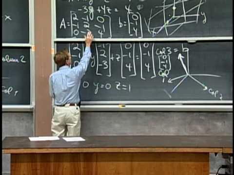
Strang Replaces Row Equations With Column Vectors to Test Solvability

斯特朗以列向量替代行方程以检验线性方程组的可解性 仅当矩阵的列保持独立并张成整个维数空间时，线性系统才能对任意右端项均有解，这使得矩阵乘法本质上是列向量的线性组合而非行点积。 吉尔伯特·斯特朗教授介绍了线性代数的核心问题：求解形如 $Ax = b$ 的线性方程组。他将相交直线与平面的常见行图像与更具基础性的列图像进行了对比，在列图像中，该系统被视作列向量的线性组合。利用2×2、3×3及更高维度的系统，斯特朗阐释了线性无关的列如何张成整个空间以确保对任意目标向量都有解，而相关或共面的列则会导致奇异、不可逆的矩阵。最后，他将矩阵-向量乘法重新定义为矩阵各列的线性组合，而不仅是行点积。 吉尔伯特·斯特朗开启了麻省理工学院的18.06线性代数课程，重点通过三个统一的视角——行图像、列图像和矩阵形式 Ax = b——来求解包含 n 个未知数的 n 个线性方程组。 (0:08) 斯特朗强调列图像是本课程最核心的概念，并将矩阵-向量乘法 Ax 定义为矩阵 A 各列的线性组合。 (8:39) 线性系统 Ax = b 对任意目标向量 b 均有解的充要条件是其列向量张成整个空间；共面或线性相关的列会将解限制在更低维的子空间中，从而导致矩阵成为奇异且不可逆的矩阵。 (27:48) 虽然通过行点积计算 Ax 可以得到相同的数值结果，但从列的角度看待乘法则阐明了任意维度下的几何可解性，并为高斯消元法奠定了概念基础。 (35:33)

In the opening lecture of MIT's 18.06 course, Gilbert Strang frames linear algebra around solving balanced systems of linear equations ($Ax = b$), contrasting the geometric limitations of the traditional row picture against the structural power of the column picture. Row Picture Versus Column Picture (4:20) A system of $n$ linear equations with $n$ unknowns can be analyzed through two distinct geometric perspectives. In the row picture, each equation represents a geometric locus—a line in two dimensions or a flat plane in three dimensions—and the solution corresponds to the common intersection point. While visualizing two lines meeting at $(1, 2)$ in the system $2x - y = 0$ and $-x + 2y = 3$ is intuitive, this perspective becomes visually cumbersome in three dimensions and impractical in higher dimensions. Linear Combinations as the Foundational Operation (8:39) The column picture groups coefficients by variable into column vectors, transforming the system into $x_1(\text{column 1}) + \dots + x_n(\text{column } n) = b$. Strang emphasizes that a linear combination—scaling vectors and adding them together—is the most fundamental operation in linear algebra. When computing the matrix-vector product $Ax$, viewing the operation as a linear combination of the columns of $A$ weighted by the components of $x$ reveals system solutions directly when $b$ aligns with known combinations of columns, unlike entry-by-entry row dot products. Column Independence and System Solvability (27:48) The question of whether $Ax = b$ can be solved for every vector $b$ hinges on whether the column vectors span the entire space. For a $3 \times 3$ matrix, if the three column vectors do not lie in a common plane, their linear combinations fill all of $\mathbb{R}^3$, making the matrix invertible and non-singular. However, if the columns are dependent—such as when the third column is the sum of the first two—their combinations remain confined to a two-dimensional plane, leaving any target vector $b$ outside that plane with no solution. Extending Column Geometry to Higher Dimensions (32:27) This geometric principle extends directly to higher dimensions where mental visualization fails. In a nine-equation system with nine unknowns, solving $Ax = b$ requires finding a linear combination of nine vectors in nine-dimensional space. While a random $9 \times 9$ matrix generated in software like MATLAB is virtually guaranteed to be independent and invertible, dependent columns—such as an identical eighth and ninth column—trap all possible combinations inside an eight-dimensional hyperplane, creating unreachable target vectors. While inspection and geometric intuition suffice for small, constructed examples, Strang concludes that arbitrary systems require a systematic algorithmic approach, previewing Gaussian elimination as the standard computational method.

麻省理工学院教授 Gilbert Strang 在 18.06 线性代数首讲中提出，求解 $n$ 元线性方程组 $Ax = b$ 是整门课程的核心任务；相较于直观展示几何交点的“行视图”（Row Picture），将方程组视为列向量线性组合的“列视图”（Column Picture）不仅是理解矩阵乘法的根本途径，更是判断系统在任意右侧向量下是否可解的基石。 行视图的几何直观与高维维数限制 (4:20) Strang 首先通过具体的方程组展开几何与代数表示。在二元系统 $2x - y = 0$ 与 $-x + 2y = 3$ 中，行视图将每个方程视为二维平面上的一条直线：第一条线穿过原点 $(0,0)$ 与点 $(1,2)$，第二条线穿过 $(-3,0)$ 与 $(1,2)$，两线交于唯一的解点 $(1,2)$。当系统扩展至三元系统（包含 $2x - y = 0$、$-x + 2y - z = -1$ 以及 $-3y + 4z = 4$）时，系数矩阵 $A$ 与未知向量 $x$、常数向量 $b = [0, -1, 4]^T$ 构成代数矩阵形式 $Ax = b$。此时每个方程在三维空间中代表一个平面，前两个平面相交成一条直线，第三个平面则与该直线相交于唯一的解点 $(0,0,1)$。 然而，Strang 指出行视图在高维空间中面临严重的直觉瓶颈。在二维平面中观察两条直线交点十分轻松，但在三维空间中辨识三个平面的相交位置已颇为吃力；一旦变量增加到四维甚至更高维度，几何超平面的相交在视觉上将完全无法呈现，迫使分析必须转向更具扩展性的代数与向量视角。 列视图与线性组合的核心地位 (8:39) Strang 将列视图列为整门课程最重要的切入点。在列视图下，二元系统被改写为列向量的线性组合：$x [2, -1]^T + y [-1, 2]^T = [0, 3]^T$。所谓线性组合，即对向量分别乘以标量系数并执行向量加法；在几何上，首个向量按比例缩放后首尾相接叠加第二个向量，最终精准到达目标向量 $b = [0, 3]^T$。由于这两个列向量指向不同方向，它们的所有可能线性组合能够铺满整个二维平面。 在三元系统中，方程同样表达为三个三维列向量以 $x, y, z$ 为权重的线性组合。当目标向量 $b$ 恰好等于第三个列向量 $[0, -1, 4]^T$ 时，无需计算即可通过直接观察得出解为 $(0, 0, 1)$；若将 $b$ 换为前两列之和 $[1, 1, -3]^T$，解立即变为 $(1, 1, 0)$。Strang 强调，在行视图中改变常数项 $b$ 会导致各个平面平移，而在列视图中，基础列向量始终保持固定，改变的仅仅是组合这些向量所需的系数权重。 向量相关性、空间填充与奇异性 (27:48) Strang 将方程组求解引向核心理论问题：“对于每一个右侧向量 $b$，方程 $Ax = b$ 是否都有解？”这在列视图中等价于询问“列向量的线性组合能否填满整个空间”。当矩阵的列向量能够张成完整的空间（如三维中的全部空间）时，该矩阵是非奇异且可逆的，对任意目标向量 $b$ 均存在解。 反之，若列向量之间存在依赖关系，系统便会退化。以三维为例，若第三个列向量恰好落在前两个列向量所张成的二维平面内（如第三列等于前两列相加），则三者所有线性组合都将被局限在该二维平面中；对于落在该平面外的任何向量 $b$，方程均无解，矩阵因而呈现奇异且不可逆的状态。将此逻辑推广至九维空间（9 个方程与 9 个未知数），如果在 MATLAB 中随机生成一个 $9 \times 9$ 矩阵，其各列几乎必然相互独立并填满九维空间；但若第九列与第八列完全相同，其组合将被限制在九维空间内的一个八维超平面上，导致绝大多数目标向量无法被到达。 矩阵乘向量的运算机制与消元展望 (35:33) 在建立了几何直觉后，Strang 重新审视了矩阵与向量乘法 $Ax$ 的代数本质。以 $2 \times 2$ 矩阵 $[[2, 5], [1, 3]]$ 乘以向量 $[1, 2]^T$ 为例，常规的行计算方式是分别计算矩阵每一行与向量的点积，即 $2(1) + 5(2) = 12$ 与 $1(1) + 3(2) = 7$。然而，Strang 极力主张采用列视角来理解该运算：$Ax$ 本质上是用向量的各个分量作为标量权重，对矩阵的各个列向量求线性组合，即 $1 [2, 1]^T + 2 [5, 3]^T = [12, 7]^T$。 列视角清晰地将矩阵运算与几何组合统一起来：如果输出目标向量为 $[12, 7]^T$，则解向量立即呈现为 $[1, 2]^T$。讲座最后指出，虽然精心构造的简单系统可以通过观察法一眼看穿，但在工程与科学计算的真实生产软件中，求解大型未知系统必须依赖系统化的通用算法。下一讲将从列组合的直观判断转向机械化计算，正式引入高斯消元法。 Strang 在首讲中确立了线性代数以列向量线性组合为基石的教学主线，论证了矩阵可逆性与列空间维度的紧密联系。尽管本讲依靠特例直观展示了几何意义与解的存在性，但对于非特定构造的通用线性方程组，如何程序化判定可解性并求出精确数值解，仍有待下一讲关于高斯消元法的系统展开。

## Background 本视频由 MIT OpenCourseWare 于 2009 年 5 月 7 日发布在 YouTube 平台上，内容为麻省理工学院数学系吉尔伯特·斯特朗（Gilbert Strang）教授在 2005 年春季主讲的 18.06 线性代数课程第一讲。根据页面简介，本讲主题为“线性方程组的几何学”（The Geometry of Linear Equations），课程配套资源及完整教学大纲均可通过 MIT 开放课程官网获取。 ## TL;DR 斯特朗教授在开篇指明，整门线性代数的核心任务是求解线性方程组 $Ax = b$。他通过二元和三元方程算例，对比了传统的“行图像”（直线或平面的空间相交）与更为根本的“列图像”（列向量的线性组合），并展示了矩阵乘向量本质上是对各列赋予权重的叠加过程。此外，他还引导学生从几何角度思考方程的可解性：当矩阵的列向量能够填满整个空间（非奇异、可逆）时，方程对任意常数向量均有解；而当列向量共面退化（奇异）时，则会导致系统失效。最后，教授将这种几何直觉拓展至九维高维空间，并为后续的标准算法——高斯消元法埋下伏笔。 ## Atmosphere & style 整堂课洋溢着经典的 MIT 实体课堂魅力，斯特朗教授举手投足间展现出大师级的亲和力与教学从容感。他的讲授不依赖复杂的幻灯片，而是通过粉笔在黑板上逐步勾勒向量与平面，期间还会幽默地自嘲“画功不如伦勃朗”，引得台下会心一笑。整堂课的节奏明快且极具启发性，教授不断通过提问引导学生跳出死记硬背的代数算式，转而建立对多维几何空间的直观想象，观感既生动亲切又发人深省。 ## Bulletin - [00:08](https://www.youtube.com/watch?v=ZK3O402wf1c&t=8s) 吉尔伯特·斯特朗教授开启 MIT 18.06 线性代数课程，指出线性代数的最根本问题是求解形如 Ax = b 的线性方程组，并对比了行图像、列图像与矩阵代数三种观察视角。 - [08:39](https://www.youtube.com/watch?v=ZK3O402wf1c&t=519s) 斯特朗强调矩阵与向量的乘积 Ax 本质上是矩阵各列的线性组合，并将列图像视为贯穿整门课程最根本的几何与代数操作。 - [27:48](https://www.youtube.com/watch?v=ZK3O402wf1c&t=1668s) 系统 Ax = b 对任意目标向量 b 是否有解，完全取决于矩阵各列的线性组合能否填满整个目标空间；列向量共面会导致矩阵奇异且不可逆。 - [32:25](https://www.youtube.com/watch?v=ZK3O402wf1c&t=1945s) 在高维空间（如 9×9 矩阵）中，随机选取的列向量极大概率保持线性无关，但若存在列相关性，组合将退化至低维超平面内，导致通用解法失效。 ## Key takeaways - [00:08](https://www.youtube.com/watch?v=ZK3O402wf1c&t=8s) 求解线性方程组是线性代数最根本的核心问题，课程主要从未知数与方程数相等的 n×n 标准系统展开。 - [00:08](https://www.youtube.com/watch?v=ZK3O402wf1c&t=8s) 观察线性方程组存在三种核心视角：行图像（直线或平面相交）、列图像（列向量线性组合）与矩阵代数形式 Ax = b。 - [02:17](https://www.youtube.com/watch?v=ZK3O402wf1c&t=137s) 在二维二元系统中，行图像表现为两条直线的交点，以此为基础建立对方程组解的几何直觉。 - [08:39](https://www.youtube.com/watch?v=ZK3O402wf1c&t=519s) 列图像将求解方程转化为寻找矩阵列向量的线性组合来合成右侧常数向量 b，该操作是整门课程的基石。 - [08:39](https://www.youtube.com/watch?v=ZK3O402wf1c&t=519s) 在优良的二维情况下，两个线性无关的列向量的所有可能线性组合能够填满整个二维平面。 - [15:19](https://www.youtube.com/watch?v=ZK3O402wf1c&t=919s) 在三维三元系统中，行图像对应三个平面两两相交并最终交于唯一解点，但高维下几何可视化难度急剧上升。 - [22:04](https://www.youtube.com/watch?v=ZK3O402wf1c&t=1324s) 相较于复杂的行图像交点，列图像通过列向量的加权叠加直观展现解的构成，在结构上更清晰稳定。 - [27:48](https://www.youtube.com/watch?v=ZK3O402wf1c&t=1668s) 方程组对任意常数项 b 均有解的充要几何条件，是矩阵所有列向量的线性组合能够张成并填满整个多维空间。 - [27:48](https://www.youtube.com/watch?v=ZK3O402wf1c&t=1668s) 能够覆盖全空间的矩阵被称为非奇异矩阵或可逆矩阵；若列向量共面，则组合被局限在子空间内，成为奇异且不可逆的情形。 - [31:28](https://www.youtube.com/watch?v=ZK3O402wf1c&t=1888s) 当列向量之间存在依赖关系（如第三列等于前两列之和）时，绝大多数外部向量 b 将不可达，方程组无解。 - [32:25](https://www.youtube.com/watch?v=ZK3O402wf1c&t=1945s) 对于 9×9 等高维系统，随机生成的矩阵在概率上几乎必然是非奇异且可逆的，而丢失维度的列组合只能局限在超平面内。 - [35:32](https://www.youtube.com/watch?v=ZK3O402wf1c&t=2132s) 计算矩阵乘向量 Ax 有两种方式：常规的按行与向量做点积，以及更具全局结构意义的按列进行线性组合。 ## Detailed walkthrough ### [00:08](https://www.youtube.com/watch?v=ZK3O402wf1c&t=8s) 课程介绍与线性方程组的引入 麻省理工学院（MIT）数学系教授吉尔伯特·斯特朗（Gilbert Strang）开启了 18.06 线性代数课程的第一讲。他开门见山地介绍了课程使用的教材《线性代数导论》（*Introduction to Linear Algebra*），并说明了包含过往练习题、MATLAB 代码和教学大纲的课程官方主页（`web.mit.edu/18.06`）。斯特朗明确指出，整门课程的核心在于解决最基础的问题：“线性代数最根本的问题，就是求解线性方程组。”（“The fundamental problem of linear algebra, which is to solve a system of linear equations.”）。本讲计划从最标准、最良好的情况入手，即未知数个数与方程个数相等的 $n \times n$ 情况。 为了剖析线性方程组，斯特朗提出了三种观察视角：第一种是大家最熟悉的“行图像”（Row picture），即一次看一个方程，在二维平面上表现为直线相交；第二种他特别打上星号强调，称其更为关键且学生可能初次接触的“列图像”（Column picture），即一次关注矩阵的一列；第三种则是纯粹的代数视角，即将方程组写成矩阵形式 $Ax = b$。斯特朗强调，整个学期的学习模式都将是先通过具体算例切入，再从中抽象出深层的数学结构。 - 课程编号：MIT 18.06（线性代数），主讲人：Gilbert Strang 教授 - 核心教材：《Introduction to Linear Algebra》 - 课程网址：`web.mit.edu/18.06` - 探讨前提：$n$ 个方程对应 $n$ 个未知数（$n \times n$ 线性系统） ```mermaid flowchart LR accTitle: 线性方程组的三种视角 accDescr: 展示求解线性方程组时的行图像、列图像和矩阵代数形式这三种不同的观察维度。 subgraph S1["观察视角"] direction TB R["行图像<br>(Row Picture)"] C["列图像<br>(Column Picture)"] M["矩阵形式<br>(Matrix Form)"] end System["线性方程组<br>Ax = b"] --> R System --> C System --> M ``` --- ### [02:17](https://www.youtube.com/watch?v=ZK3O402wf1c&t=137s) 矩阵代数形式与二元方程组的行图像 斯特朗给出了一个简单的二元一次方程组作为切入示例： $$2x - y = 0$$ $$-x + 2y = 3$$ 在画图之前，他便按捺不住先将其转换为矩阵代数形式 $Ax = b$。其中系数矩阵 $A$ 是一个两行两列的数阵，第一行为 $2$ 和 $-1$，第二行为 $-1$ 和 $2$；未知数向量 $x$ 包含分量 $x$ 与 $y$；等号右侧常数项则组成向量 $b = \begin{bmatrix} 0 \\ 3 \end{bmatrix}$。 紧接着，斯特朗绘制了该系统的“行图像”。在 $xy$ 平面上，第一行方程 $2x - y = 0$ 恒过原点 $(0,0)$，并且当 $x = 1$ 时 $y = 2$，连线便得到了该方程所代表的直线。对于第二行方程 $-x + 2y = 3$，由于右端项非零，该直线不过原点：当 $y = 0$ 时可求得 $x = -3$；当 $x = -1$ 时，代入可得 $y = 1$。将这两点相连得到第二条直线。两条直线的交点即为方程组的解。斯特朗验证道，点 $(1, 2)$ 完美契合两个方程：“如果 $x$ 等于 1，$y$ 等于 2，那么 $-1 + 4 = 3$，完全正确。”尽管这种几何图像学生早前已见过多次，但斯特朗特别声明，从 $n = 2$ 的行图像开始，是建立几何直觉不可或缺的第一步。 - 系数矩阵 $A$：$\begin{bmatrix} 2 & -1 \\ -1 & 2 \end{bmatrix}$ - 未知数向量 $x$：$\begin{bmatrix} x \\ y \end{bmatrix}$，常数向量 $b$：$\begin{bmatrix} 0 \\ 3 \end{bmatrix}$ - 行方程一：$2x - y = 0$（过点 $(0,0)$ 与 $(1,2)$ 的直线） - 行方程二：$-x + 2y = 3$（过点 $(-3,0)$ 与 $(-1,1)$ 的直线） - 几何交点（唯一解）：$x = 1,\ y = 2$ --- ### [08:39](https://www.youtube.com/watch?v=ZK3O402wf1c&t=519s) 列图像与列向量的线性组合 完成行图像后，斯特朗正式切入整堂课的核心要点——列图像（Column picture）。他将原方程组重新整理为向量相加的形式： $$x \begin{bmatrix} 2 \\ -1 \end{bmatrix} + y \begin{bmatrix} -1 \\ 2 \end{bmatrix} = \begin{bmatrix} 0 \\ 3 \end{bmatrix}$$ 斯特朗向全场强调这一视角的重大意义：“这被称为线性组合，它是全课程中最根本的操作。”（“This is called a linear combination. And it's the most fundamental operation in the whole course.”）。他指出，方程的本质就是寻找第一列向量 $\begin{bmatrix} 2 \\ -1 \end{bmatrix}$ 与第二列向量 $\begin{bmatrix} -1 \\ 2 \end{bmatrix}$ 的合适线性组合，以精确合成目标向量 $b = \begin{bmatrix} 0 \\ 3 \end{bmatrix}$。 在几何画板上，斯特朗绘制了这两个列向量：第一列向右 2、向下 1；第二列向左 1、向上 2。借助之前求得的解，他选择直接取“1 个第一列”加上“2 个第二列”。他以向量首尾相接的方式演示加法：从原点出发画出 1 个第一列，在其箭头末端接上第 1 个第二列（虚线向左 1、向上 2），再连续接上第 2 个第二列。最终箭头的终点准确落在了水平位移为 $0$、垂直高度为 $3$ 的位置，即向量 $\begin{bmatrix} 0 \\ 3 \end{bmatrix}$。 ```mermaid flowchart TD accTitle: 列向量线性组合过程 accDescr: 展示将第一列向量与两个第二列向量通过首尾相接方式合成为目标向量b的几何步骤。 Start["起点 (0, 0)"] -->|"1 × 列1: (2, -1)"| V1["(2, -1)"] V1 -->|"1 × 列2: (-1, 2)"| V2["(1, 1)"] V2 -->|"1 × 列2: (-1, 2)"| Target["目标向量 b: (0, 3)"] ``` 在展示完这一几何组合后，斯特朗抛出了一个将贯穿整个学期的核心议题：如果遍历所有的标量 $x$ 和 $y$，取遍这两个列向量的所有可能组合，会得到什么？他给出结论并提醒学生牢记：“这两个列向量的所有可能组合将填满整个二维平面。”（“The combinations of this and this would fill the whole plane.”）。这也意味着对于任意给定的右端项向量 $b$，该方程组在二维空间中都将能找到对应的解。 ### [15:19](https://www.youtube.com/watch?v=ZK3O402wf1c&t=919s) 拓展到三元一次方程组：行图像（平面相交） Gilbert Strang 教授将视角从简单的二元一次方程组扩展到了三元方程组。为了让学生直观地看清二维与三维的过渡，他在黑板上写下了一个具体的 $3 \times 3$ 线性方程组： $$\begin{aligned} 2x - y + 0z &= 0 \\ -x + 2y - z &= -1 \\ 0x - 3y + 4z &= 4 \end{aligned}$$ 教授将这组方程写成了紧凑的矩阵形式 $Ax = b$。矩阵 $A$ 的三行分别由系数提取而成：第一行为 $[2, -1, 0]$，第二行为 $[-1, 2, -1]$，第三行为 $[0, -3, 4]$；右侧常数向量 $b$ 则为 $[0, -1, 4]^T$。在着手求解之前，Strang 强调核心在于“理解这些方程，然后再去解它们”。理解的第一种途径是**行图像（row picture）**。在三维直角坐标系 $(x, y, z)$ 中，每一个线性方程的几何图形都是一个平面。 ```mermaid flowchart TD accTitle: Row picture of 3x3 system accDescr: Visualizing how three planes intersect in a 3D system to form a unique point solution. subgraph RowPicture["行图像（Row Picture）"] E1["方程 1: 平面 1"] E2["方程 2: 平面 2"] E3["方程 3: 平面 3"] Line["两平面相交成一条直线"] Point["三平面相交于一个解点 (x, y, z)"] E1 --> Line E2 --> Line Line --> Point E3 --> Point end ``` 为了画出第二号方程 $-x + 2y - z = -1$ 所代表的平面，Strang 在坐标轴上逐一寻找满足条件的点。由于原点 $(0,0,0)$ 代入并不成立，他试探出点 $(1,0,0)$，接着令 $x=0, y=0$ 得到 $(0,0,1)$，最后令 $x=0, z=0$ 算得 $y = -\frac{1}{2}$。三点确定一个平面，但由于在黑板上画立体图十分困难，Strang 自嘲道：“三点确定一个平面，但你们的授课老师可不是伦勃朗，画功在这里可是个弱项。”（“These three points determine a plane, but your lecturer is not Rembrandt and the art is going to be the weak point here.”）他勾勒出第一个方程和第二个方程的平面相交形成一条直线，而第三个方程的平面穿过这条直线，最终相交于唯一的一点。虽然行图像理论上很清晰，但随着维度上升，平面相交的空间图景变得极其模糊难辨，因此教授坦言自己更偏爱**列图像（column picture）**。 - 矩阵 $A$ 为三阶方阵： $$\begin{bmatrix} 2 & -1 & 0 \\ -1 & 2 & -1 \\ 0 & -3 & 4 \end{bmatrix}$$ - 右侧常数向量 $b = \begin{bmatrix} 0 \\ -1 \\ 4 \end{bmatrix}$ - 行图像的核心几何意义：每一个方程对应一个三维平面，前两个平面相交成一条直线，第三个平面与该直线交于一个确定解的点。 --- ### [22:04](https://www.youtube.com/watch?v=ZK3O402wf1c&t=1324s) 列图像：向量线性组合的视角 随后，Strang 将同一个问题转换为列图像。三元方程组被重新表达为三维列向量的线性组合： $$x \begin{bmatrix} 2 \\ -1 \\ 0 \end{bmatrix} + y \begin{bmatrix} -1 \\ 2 \\ -3 \end{bmatrix} + z \begin{bmatrix} 0 \\ -1 \\ 4 \end{bmatrix} = \begin{bmatrix} 0 \\ -1 \\ 4 \end{bmatrix}$$ 在这幅图景中，问题的本质演变为：我们要寻找怎样的标量组合系数 $x, y, z$，才能利用矩阵的三个列向量拼接出右侧的目标向量 $b$。Strang 指出，这道题目是自己为了演示而特意设计的：右侧向量 $b = [0, -1, 4]^T$ 恰好与矩阵的第三列一模一样。因此，答案一目了然：取 0 个第一列，0 个第二列，以及 1 个第三列。也就是说，解就是 $(x, y, z) = (0, 0, 1)$。这个解恰好对应了此前在行图像中由于画图困难而未能肉眼看出的“三面交点”。 ```mermaid flowchart LR accTitle: Column picture linear combination accDescr: Combining three column vectors with weights to produce vector b. subgraph Columns["矩阵 A 的三列"] C1["col 1: [2, -1, 0]ᵀ"] C2["col 2: [-1, 2, -3]ᵀ"] C3["col 3: [0, -1, 4]ᵀ"] end subgraph Combo["线性组合"] X["x = 0"] Y["y = 0"] Z["z = 1"] end Target["目标向量 b: [0, -1, 4]ᵀ"] C1 -.->|* 0| Combo C2 -.->|* 0| Combo C3 -->|* 1| Combo Combo --> Target ``` 针对更通用的情况，Strang 预告接下来的课程将系统讲解高斯消元法（elimination），这是所有大型科学计算软件求解线性方程组的核心基础算法。为了进一步巩固列图像的直观性，Strang 现场又换了一个特别设计的右端项：将第一列与第二列相加，得到新向量 $b' = [1, 1, -3]^T$。在新的方程组下，由于 $1 \cdot (\text{col 1}) + 1 \cdot (\text{col 2}) + 0 \cdot (\text{col 3}) = b'$，解直接跳变为了 $(1, 1, 0)$。在行图像中，这意味着换了三个全新的平面相交于新点；而在列图像中，基底列向量完全没有变，只是改变了它们线性叠加的权重。 --- ### [27:48](https://www.youtube.com/watch?v=ZK3O402wf1c&t=1668s) 核心思考：能否对任意右侧向量 $b$ 求解？ 在讨论完具体解后，Strang 引导全班转向本门课程最核心的宏观思考（big picture）：“我们能否对每一个右端项 $b$ 都求解这个方程组？”也就是说，方程 $Ax = b$ 是否对任意三维空间中的向量 $b$ 都有解？ 教授强调，代数问题“是否存在解”等价于几何语言：“这些列向量的所有可能线性组合，是否能够填满整个三维空间？”（“Do the linear combinations of the columns fill three dimensional space?”）。当矩阵 $A$ 乘以向量 $x$ 时，本质上就是在对 $A$ 的列进行线性组合。如果这些列向量的组合能够覆盖整个 $\mathbb{R}^3$ 空间，那么无论给定什么样的 $b$，我们都必定能找到对应的解 $x$。 ```mermaid flowchart TD accTitle: Solvability condition for Ax equals b accDescr: The conditions under which Ax = b is solvable for all b versus when it fails. Q{"列向量能否填满三维空间？"} Q -->|"是（良好情形）"| Good["非奇异矩阵 / 可逆矩阵"] Good --> Solvable["对任意 b，Ax = b 均有唯一解"] Q -->|"否（退化情形）"| Bad["三列向量共面（共面导致降维）"] Bad --> Plane["所有线性组合仅局限在一个二维平面上"] Plane --> Unsolvable["若 b 落在该平面外，则方程无解"] ``` 对于当前给出的矩阵 $A$，Strang 给出了肯定的回答：它的列向量确实能填满三维空间，因此它是一个“优良的矩阵（good matrix）”，在数学术语中被称为**非奇异矩阵（non-singular matrix）**或**可逆矩阵（invertible matrix）**。那么，事情在什么时候会变糟？Strang 引发学生思考：“如果这三个列向量全部落在同一个平面内，那么它们的线性组合也将被锁死在同一个平面里。”（“If these three columns all lie in the same plane, then their combinations will lie in that same plane.”）。一旦三个向量共面，它们就无法张成完整的三维空间；如果外部给定的向量 $b$ 恰好漂浮在该平面之外，线性组合便无论如何也无法触及它，消元法就会在此失效，方程组也将无解。这一几何直观为后续深入学习线性相关性与奇异矩阵埋下了关键伏笔。 ### [31:28](https://www.youtube.com/watch?v=ZK3O402wf1c&t=1888s) 线性相关与奇异矩阵：当列向量落在同一平面时 吉尔伯特·斯特朗（Gilbert Strang）教授深入探讨了线性方程组可能失效的退化情形。在三维空间中，如果第三个列向量恰好是第一列与第二列的和，整个方程组就会陷入麻烦。由于第三列完全落在了由前两个列向量张成的平面内，它并没有为我们带来任何全新的空间维度或方向。因此，这三个列向量无论怎么进行线性组合，其结果都只能被局限在这个二维平面内部。 当右端向量 $b$ 恰好落在这个平面上时，方程组尚有解可寻；但三维空间中绝大多数的 $b$ 都会漂浮在平面之外，因而是根本无法通过组合触达的。这种情形正是矩阵代数中的“奇异矩阵”（singular matrix），意味着该矩阵是不可逆的（not invertible），也无法保证对任意的 $b$ 都有解。正如斯特朗教授所断言的那样：“So that would be a singular case. The matrix would be not invertible. There would not be a solution for every b.” - 若第 3 列为第 1 列与第 2 列的和（$col_3 = col_1 + col_2$），则所有线性组合被限制在二维平面内。 - 只有落在该平面内的右端项 $b$ 才能求解；平面外的绝大部分 $b$ 均不可解。 - 该情况属于奇异情况（singular case），矩阵不可逆（not invertible）。 ```mermaid flowchart TD accTitle: 奇异矩阵与列向量线性组合 accDescr: 展示当列向量线性相关时，所有线性组合被局限在子空间内，导致外部向量不可达。 subgraph SingularMatrix["奇异矩阵 (退化情形)"] C1["列 1 (Column 1)"] C2["列 2 (Column 2)"] C3["列 3 = 列 1 + 列 2<br/>(无新维度)"] end subgraph Space["向量空间覆盖"] Plane["二维平面组合<br/>(无法填满整个三维空间)"] Solvable["平面内的 b<br/>(有解)"] Unsolvable["平面外的绝大多数 b<br/>(无解 / 不可达)"] end C1 --> Plane C2 --> Plane C3 --> Plane Plane --> Solvable Plane -.->|无法触达| Unsolvable ``` ### [32:25](https://www.youtube.com/watch?v=ZK3O402wf1c&t=1945s) 九维空间中的想象力与线性无关性 斯特朗教授带领学生尝试思考九维空间（9-dimensional space）的情形。对于含有九个方程和九个未知数的线性系统，矩阵由九个九维列向量构成，我们所做的依旧是寻找这九个向量的线性组合来命中目标向量 $b$。教授坦承自己也无法真正在脑海中将九维实体具象化，但他鼓励大家假装自己能看到，因为这就是线性代数的思维方式。 当我们提问“是否对每一个九维向量 $b$ 都能求解”时，答案完全取决于这九个列向量的性质。如果在 MATLAB 中输入 `rand` 随机生成一个 $9 \times 9$ 的矩阵，由于随机选取的列向量极大概率是线性无关的，教授打赌这必定是一个非奇异的、完美的、可逆的良好矩阵。但如果人为设计让第九列完全等于第八列，那么第九列就没有贡献任何新方向，所有线性组合便只能填满九维空间中的一个“八维超平面”（an eight-dimensional plane），绝大多数九维向量都将无法表示。斯特朗教授指出，习惯这种在高维空间中运算的思维正是该课程的核心：“That's really the central thought -- that you get kind of used to in linear algebra.” - $9 \times 9$ 系统对应 9 维空间中 9 个列向量的线性组合。 - 在 MATLAB 中调用随机指令生成的 $9 \times 9$ 矩阵几乎必然是非奇异（non-singular）且可逆的（invertible）。 - 若第 9 列与第 8 列相同，则缺失一个独立自由度，所有线性组合仅构成 9 维空间中的一个“8 维平面”，无法覆盖整个空间。 ### [35:32](https://www.youtube.com/watch?v=ZK3O402wf1c&t=2132s) 矩阵乘向量的本质：列的线性组合与行内积 斯特朗教授将之前的几何直觉落实为具体的代数符号，写下了核心方程 $Ax = b$。为了说明矩阵与向量的乘法运算，他构造了一个简单的 $2 \times 2$ 算例： $$\begin{bmatrix} 2 & 5 \\ 1 & 3 \end{bmatrix} \begin{bmatrix} 1 \\ 2 \end{bmatrix}$$ 教授特别强调了他最推崇的理解方式——“按列进行”（a column at a time）。按这种视角，矩阵乘以向量本质上是用向量的各个分量作为权重，对矩阵的各个列做线性组合，即 1 倍的第一列加上 2 倍的第二列： $$1 \begin{bmatrix} 2 \\ 1 \end{bmatrix} + 2 \begin{bmatrix} 5 \\ 3 \end{bmatrix} = \begin{bmatrix} 2 + 10 \\ 1 + 6 \end{bmatrix} = \begin{bmatrix} 12 \\ 7 \end{bmatrix}$$ 随后教授提到了另一种更为大家所熟知的方式——“按行进行”（a row at a time）。这种算法通过将矩阵的每一行看作行向量，与列向量 $x$ 做点积（dot product）：第一行计算为 $2 \times 1 + 5 \times 2 = 12$，第二行计算为 $1 \times 1 + 3 \times 2 = 7$。虽然两种方式计算结果完全相同，但教授郑重其事地强调了理解列组合的重要性：“A times x is a combination of the columns of A. That's how I hope you will think of A times x when we need it.”如果右端向量 $b$ 恰好是 $\begin{bmatrix} 12 \\ 7 \end{bmatrix}$，那么对应的解 $x$ 自然就是 $\begin{bmatrix} 1 \\ 2 \end{bmatrix}$。最后，教授预告下一节课将正式讲解利用消元法（elimination）系统化求解任意规模线性方程组的标准流程。 - 矩阵乘法 $Ax$ 的两种视角对比： - **按列看待（线性组合视角）**：$x$ 的各分量作为系数，对 $A$ 的各列进行线性组合。 - **按行看待（点积视角）**：用 $A$ 的每一行与向量 $x$ 分别做点积（dot product）。 - 若线性方程组为 $\begin{bmatrix} 2 & 5 \\ 1 & 3 \end{bmatrix} \begin{bmatrix} x_1 \\ x_2 \end{bmatrix} = \begin{bmatrix} 12 \\ 7 \end{bmatrix}$，其显而易见的解为 $x = \begin{bmatrix} 1 \\ 2 \end{bmatrix}$。 - 下堂课预告：引入消元法（elimination）系统化求解通用线性系统。 ## Notable quotes > [00:08](https://www.youtube.com/watch?v=ZK3O402wf1c&t=8s) 线性代数最根本的问题，就是求解线性方程组。 — 吉尔伯特·斯特朗 ## Mentioned Gilbert Strang, MIT, MATLAB, Introduction to Linear Algebra, 伦勃朗 ## Video description Lecture 1: The Geometry of Linear Equations. View the complete course at: http://ocw.mit.edu/18-06S05 License: Creative Commons BY-NC-SA More information at http://ocw.mit.edu/terms More courses at http://ocw.mit.edu [Source](https://www.youtube.com/watch?v=ZK3O402wf1c)

[0:08] 吉尔伯特·斯特朗: 线性代数最根本的问题，就是求解线性方程组。

[35:33] Gilbert Strang: A times x is a combination of the columns of A. [15:19] Gilbert Strang: The row picture was a cinch when we looked at two lines meeting. When we look at three planes meeting, it's not so clear and in four dimensions probably a little less clear.

[0:08] Hi. [0:09] This is the first lecture in MIT's course 18.06, [0:14] linear algebra, and I'm Gilbert Strang. [0:19] The text for the course is this book, [0:23] Introduction to Linear Algebra. [0:26] And the course web page, which has got a lot of exercises from [0:32] the past, MatLab codes, the syllabus for the course, [0:38] is web.mit.edu/18.06. [0:44] And this is the first lecture, lecture one. [0:49] So, and later we'll give the web address for viewing these, [0:55] videotapes. [0:57] Okay, so what's in the first lecture? [1:02] This is my plan. [1:05] The fundamental problem of linear algebra, [1:09] which is to solve a system of linear equations. [1:13] So let's start with a case when we [1:16] have some number of equations, say n equations and n unknowns. [1:21] So an equal number of equations and unknowns. [1:23] That's the normal, nice case. [1:26] And what I want to do is -- with examples, of course -- [1:31] to describe, first, what I call the Row picture. [1:37] That's the picture of one equation at a time. [1:40] It's the picture you've seen before in two [1:43] by two equations where lines meet. [1:46] So in a minute, you'll see lines meeting. [1:49] The second picture, I'll put a star [1:52] beside that, because that's such an important one. [1:55] And maybe new to you is the picture -- a column at a time. [2:01] And those are the rows and columns of a matrix. [2:05] So the third -- the algebra way to look at the problem is [2:08] the matrix form and using a matrix that I'll call A. [2:13] Okay, so can I do an example? [2:17] The whole semester will be examples and then see what's [2:23] going on with the example. [2:25] So, take an example. [2:27] Two equations, two unknowns. [2:30] So let me take 2x -y =0, let's say. [2:38] And -x 2y=3. [2:45] Okay. [2:46] let me -- I can even say right away -- [2:50] what's the matrix, that is, what's the coefficient matrix? [2:57] The matrix that involves these numbers -- [3:00] a matrix is just a rectangular array of numbers. [3:05] Here it's two rows and two columns, so 2 and -- [3:09] minus 1 in the first row minus 1 and 2 in the second row, [3:14] that's the matrix. [3:16] And the right-hand -- the, unknown -- [3:21] well, we've got two unknowns. [3:23] So we've got a vector, with two components, x and y, [3:27] and we've got two right-hand sides that go into a vector [3:31] 0 3. [3:32] I couldn't resist writing the matrix form, right -- [3:38] even before the pictures. [3:41] So I always will think of this as the matrix A, [3:45] the matrix of coefficients, then there's a vector of [3:49] unknowns. [3:50] Here we've only got two unknowns. [3:51] Later we'll have any number of unknowns. [3:54] And that vector of unknowns, well I'll often -- [3:57] I'll make that x -- [3:59] extra bold. [4:01] A and the right-hand side is also a vector [4:04] that I'll always call b. [4:08] So linear equations are A x equal b and the idea now [4:13] is to solve this particular example [4:16] and then step back to see the bigger picture. [4:20] Okay, what's the picture for this example, the Row picture? [4:24] Okay, so here comes the Row picture. [4:30] So that means I take one row at a time [4:32] and I'm drawing here the xy plane [4:38] and I'm going to plot all the points that [4:43] satisfy that first equation. [4:47] So I'm looking at all the points that satisfy 2x-y =0. [4:53] It's often good to start with which point on the horizontal [4:59] line -- on this horizontal line, y is zero. [5:02] The x axis has y as zero and that -- in this case, actually, [5:06] then x is zero. [5:07] So the point, the origin -- [5:11] the point with coordinates (0,0) is on the line. [5:16] It solves that equation. [5:18] Okay, tell me in -- well, I guess I have to tell you [5:22] another point that solves this same equation. [5:26] Let me suppose x is one, so I'll take x to be one. [5:32] Then y should be two, right? [5:34] So there's the point one two that also solves this equation. [5:40] And I could put in more points. [5:42] But, but let me put in all the points [5:45] at once, because they all lie on a straight line. [5:50] This is a linear equation and that word linear [5:53] got the letters [5:54] Okay, thanks. for line in it. [5:56] That's the equation -- this is the line that ... [5:59] of solutions to 2x-y=0 my first row, first equation. [6:08] So typically, maybe, x equal a half, y equal one will work. [6:14] And sure enough it does. [6:15] Okay, that's the first one. [6:17] Now the second one is not going to go through the origin. [6:22] It's always important. [6:24] Do we go through the origin or not? [6:26] In this case, yes, because there's a zero over there. [6:30] In this case we don't go through the origin, [6:32] because if x and y are zero, we don't get three. [6:36] So, let me again say suppose y is zero, [6:40] what x do we actually get? [6:42] If y is zero, then I get x is minus three. [6:48] So if y is zero, I go along minus three. [6:52] So there's one point on this second line. [6:56] Now let me say, well, suppose x is minus one -- [7:03] just to take another x. [7:05] If x is minus one, then this is a one [7:09] and I think y should be a one, because if x is minus one, [7:15] then I think y should be a one and we'll get that point. [7:19] Is that right? [7:20] If x is minus one, that's a one. [7:23] If y is a one, that's a two and the one [7:25] and the two make three and that point's on the equation. [7:28] Okay. [7:29] Now, I should just draw the line, right, [7:31] connecting those two points at -- [7:34] that will give me the whole line. [7:36] And if I've done this reasonably well, [7:40] I think it's going to happen to go through -- well, [7:42] not happen -- it was arranged to go through that point. [7:46] So I think that the second line is this one, [7:50] and this is the all-important point that lies on both lines. [7:56] Shall we just check that that point which [7:58] is the point x equal one and y was two, right? [8:03] That's the point there and that, I believe, [8:07] solves both equations. [8:10] Let's just check this. [8:11] If x is one, I have a minus one plus four equals three, okay. [8:18] Apologies for drawing this picture [8:21] that you've seen before. [8:25] But this -- seeing the row picture -- [8:29] first of all, for n equal 2, two equations and two unknowns, [8:33] it's the right place to start. [8:35] Okay. [8:36] So we've got the solution. [8:37] The point that lies on both lines. [8:39] Now can I come to the column picture? [8:43] Pay attention, this is the key point. [8:47] So the column picture. [8:49] I'm now going to look at the columns of the matrix. [8:53] I'm going to look at this part and this part. [8:56] I'm going to say that the x part is really x times -- [9:05] you see, I'm putting the two -- [9:06] I'm kind of getting the two equations at once -- [9:10] that part and then I have a y and in the first equation [9:15] it's multiplying a minus one and in the second equation a two, [9:19] and on the right-hand side, zero and three. [9:26] You see, the columns of the matrix, the columns of A [9:29] are here and the right-hand side b is there. [9:33] And now what is the equation asking for? [9:36] It's asking us to find -- somehow to combine that vector [9:42] and this one in the right amounts to get that one. [9:47] It's asking us to find the right linear combination -- [9:51] this is called a linear combination. [9:55] And it's the most fundamental operation in the whole course. [10:01] It's a linear combination of the columns. [10:06] That's what we're seeing on the left side. [10:09] Again, I don't want to write down a big definition. [10:13] You can see what it is. [10:15] There's column one, there's column two. [10:17] I multiply by some numbers and I add. [10:21] That's a combination -- a linear combination and I want to make [10:25] those numbers the right numbers to produce zero three. [10:30] Okay. [10:32] Now I want to draw a picture that, represents what this -- [10:37] this is algebra. [10:38] What's the geometry, what's the picture that goes with it? [10:41] Okay. [10:42] So again, these vectors have two components, [10:45] so I better draw a picture like that. [10:50] So can I put down these columns? [10:52] I'll draw these columns as they are, [10:55] and then I'll do a combination of them. [10:58] So the first column is over two and down one, right? [11:04] So there's the first column. [11:06] The first column. [11:07] Column one. [11:10] It's the vector two minus one. [11:13] The second column is -- [11:18] minus one is the first component and up two. [11:22] It's here. [11:24] There's column two. [11:27] So this, again, you see what its components are. [11:32] Its components are minus one, two. [11:35] Good. [11:36] That's this guy. [11:39] Now I have to take a combination. [11:43] What combination shall I take? [11:47] Why not the right combination, what the hell? [11:50] Okay. [11:51] So the combination I'm going to take [11:53] is the right one to produce zero three [11:57] and then we'll see it happen in the picture. [11:59] So the right combination is to take x as one of those [12:04] and two of these. [12:09] It's because we already know that that's the right x and y, [12:12] so why not take the correct combination here and see it [12:15] happen? [12:16] Okay, so how do I picture this linear combination? [12:21] So I start with this vector that's already here -- [12:25] so that's one of column one, that's one times column [12:28] one, right there. [12:30] And now I want to add on -- so I'm going to hook the next [12:33] vector onto the front of the arrow will start the next [12:38] vector and it will go this way. [12:40] So let's see, can I do it right? [12:44] If I added on one of these vectors, [12:46] it would go left one and up two, so we'd go left one and up two, [12:50] so it would probably get us to there. [12:52] Maybe I'll do dotted line for that. [12:54] Okay? [12:55] That's one of column two tucked onto the end, [12:59] but I wanted to tuck on two of column two. [13:03] So that -- the second one -- we'll go up left one and up two [13:07] also. [13:07] It'll probably end there. [13:09] And there's another one. [13:10] So what I've put in here is two of column two. [13:17] Added on. [13:19] And where did I end up? [13:23] What are the coordinates of this result? [13:28] What do I get when I take one of this plus two of that? [13:32] I do get that, of course. [13:34] There it is, x is zero, y is three, that's b. [13:38] That's the answer we wanted. [13:41] And how do I do it? [13:43] You see I do it just like the first component. [13:46] I have a two and a minus two that produces a zero, [13:50] and in the second component I have a minus one and a four, [13:54] they combine to give the three. [13:57] But look at this picture. [14:01] So here's our key picture. [14:03] I combine this column and this column to get this guy. [14:10] That was the b. [14:11] That's the zero three. [14:13] Okay. [14:14] So that idea of linear combination is crucial, [14:18] and also -- [14:21] do we want to think about this question? [14:25] Sure, why not. [14:26] What are all the combinations? [14:29] If I took -- can I go back to xs and ys? [14:35] This is a question for really -- [14:38] it's going to come up over and over, [14:41] but why don't we see it once now? [14:45] If I took all the xs and all the ys, all the combinations, [14:50] what would be all the results? [14:53] And, actually, the result would be [14:56] that I could get any right-hand side at all. [14:59] The combinations of this and this [15:02] would fill the whole plane. [15:06] You can tuck that away. [15:08] We'll, explore it further. [15:14] But this idea of what linear combination gives b and what do [15:19] all the linear combinations give, [15:21] what are all the possible, achievable right-hand sides be [15:25] -- that's going to be basic. [15:26] Okay. [15:27] Can I move to three equations and three unknowns? [15:31] Because it's easy to picture the two by two case. [15:38] Let me do a three by three example. [15:40] Okay, I'll sort of start it the same way, [15:43] say maybe 2x-y and maybe I'll take no zs as a zero and maybe [15:50] a -x 2y and maybe a -z as a -- oh, [15:55] let me make that a minus one and, just for variety let me [16:01] take, -3z, -3ys, I should keep the ys in that line, [16:09] and 4zs is, say, 4. [16:14] Okay. [16:16] That's three equations. [16:19] I'm in three dimensions, x, y, z. [16:22] And, I don't have a solution yet. [16:27] So I want to understand the equations and then solve them. [16:32] Okay. [16:32] So how do I you understand them? [16:35] The row picture one way. [16:37] The column picture is another very important way. [16:41] Just let's remember the matrix form, here, [16:43] because that's easy. [16:45] The matrix form -- what's our matrix A? [16:49] Our matrix A is this right-hand side, the two and the minus one [16:54] and the zero from the first row, the minus one and the two [16:58] and the minus one from the second row, [17:00] the zero, the minus three and the four from the third row. [17:08] So it's a three by three matrix. [17:11] Three equations, three unknowns. [17:12] And what's our right-hand side? [17:14] Of course, it's the vector, zero minus one, four. [17:20] Okay. [17:21] So that's the way, well, that's the short-hand to write out [17:26] the three equations. [17:28] But it's the picture that I'm looking for today. [17:31] Okay, so the row picture. [17:32] All right, so I'm in three dimensions, x, [17:38] find out when there isn't a solution. [17:42] y and z. [17:45] And I want to take those equations one at a time and ask [17:51] -- [17:51] and make a picture of all the points that satisfy -- [17:55] let's take equation number two. [17:57] If I make a picture of all the points that satisfy -- [18:00] all the x, y, z points that solve this equation -- [18:05] well, first of all, the origin is not one of them. [18:09] x, y, z -- it being 0, 0, 0 would not solve that equation. [18:14] So what are some points that do solve the equation? [18:17] Let's see, maybe if x is one, y and z could be zero. [18:23] That would work, right? [18:24] So there's one point. [18:26] I'm looking at this second equation, [18:29] here, just, to start with. [18:33] Let's see. [18:33] Also, I guess, if z could be one, [18:36] x and y could be zero, so that would just [18:38] go straight up that axis. [18:41] And, probably I'd want a third point here. [18:46] Let me take x to be zero, z to be zero, [18:55] then y would be minus a half, right? [19:00] So there's a third point, somewhere -- oh my -- okay. [19:06] Let's see. [19:07] I want to put in all the points that satisfy that equation. [19:13] Do you know what that bunch of points will be? [19:17] It's a plane. [19:19] If we have a linear equation, then, fortunately, [19:22] the graph of the thing, the plot of all the points that solve it [19:27] are a plane. [19:30] These three points determine a plane, [19:32] but your lecturer is not Rembrandt [19:37] and the art is going to be the weak point here. [19:43] So I'm just going to draw a plane, right? [19:46] There's a plane somewhere. [19:48] That's my plane. [19:50] That plane is all the points that solves this guy. [19:54] Then, what about this one? [19:59] Two x minus y plus zero z. [20:02] So z actually can be anything. [20:05] Again, it's going to be another plane. [20:08] Each row in a three by three problem [20:11] gives us a plane in three dimensions. [20:14] So this one is going to be some other plane -- [20:17] maybe I'll try to draw it like this. [20:20] And those two planes meet in a line. [20:25] So if I have two equations, just the first two [20:29] equations in three dimensions, those give me a line. [20:33] The line where those two planes meet. [20:35] And now, the third guy is a third plane. [20:42] And it goes somewhere. [20:49] Okay, those three things meet in a point. [20:51] Now I don't know where that point is, frankly. [20:55] But -- linear algebra will find it. [20:58] The main point is that the three planes, because they're not [21:05] parallel, they're not special. [21:08] They do meet in one point and that's the solution. [21:11] But, maybe you can see that this row picture is [21:16] getting a little hard to see. [21:19] The row picture was a cinch when we looked at two lines [21:24] meeting. [21:25] When we look at three planes meeting, [21:27] it's not so clear and in four dimensions probably [21:32] a little less clear. [21:34] So, can I quit on the row picture? [21:37] Or quit on the row picture before I've successfully [21:41] found the point where the three planes meet? [21:45] All I really want to see is that the row picture consists [21:51] of three planes and, if everything works right, [21:55] three planes meet in one point and that's a solution. [21:59] Now, you can tell I prefer the column picture. [22:04] Okay, so let me take the column picture. [22:06] That's x times -- [22:09] so there were two xs in the first equation minus one x is, [22:14] and no xs in the third. [22:16] It's just the first column of that. [22:19] And how many ys are there? [22:21] There's minus one in the first equations, two in the second [22:24] and maybe minus three in the third. [22:27] Just the second column of my matrix. [22:29] And z times no zs minus one zs and four zs. [22:37] And it's those three columns, right, [22:41] that I have to combine to produce the right-hand side, [22:46] which is zero minus one four. [22:52] Okay. [22:54] So what have we got on this left-hand side? [22:57] A linear combination. [22:59] It's a linear combination now of three vectors, [23:02] and they happen to be -- each one is a three dimensional [23:05] vector, so we want to know what combination of those three [23:10] vectors produces that one. [23:12] Shall I try to draw the column picture, then? [23:15] So, since these vectors have three components -- [23:18] so it's some multiple -- let me draw in the first column [23:21] as before -- [23:23] x is two and y is minus one. [23:27] Maybe there is the first column. [23:32] y -- the second column has maybe a minus one and a two and the y [23:38] is a minus three, somewhere, there possibly, column two. [23:44] And the third column has -- [23:46] no zero minus one four, so how shall I draw that? [23:52] So this was the first component. [23:57] The second component was a minus one. [23:59] Maybe up here. [24:01] That's column three, that's the column zero minus one and four. [24:08] This guy. [24:12] So, again, what's my problem? [24:15] What this equation is asking me to do [24:18] is to combine these three vectors [24:21] with a right combination to produce this one. [24:27] Well, you can see what the right combination is, because [24:33] in this special problem, specially chosen [24:38] by the lecturer, that right-hand side that I'm trying to get [24:42] is actually one of these columns. [24:45] So I know how to get that one. [24:46] So what's the solution? [24:48] What combination will work? [24:50] I just want one of these and none of these. [24:53] So x should be zero, y should be zero and z should [24:59] be one. [25:02] That's the combination. [25:04] One of those is obviously the right one. [25:07] Column three is actually the same [25:09] as b in this particular problem. [25:15] I made it work that way just so we [25:17] would get an answer, (0,0,1), so somehow that's [25:21] the point where those three planes met [25:25] and I couldn't see it before. [25:28] Of course, I won't always be able to see it from the column [25:31] picture, either. [25:33] It's the next lecture, actually, which is about elimination, [25:39] which is the systematic way that everybody -- [25:46] every bit of software, too -- [25:51] production, large-scale software would solve the equations. [25:56] So the lecture that's coming up. [25:59] If I was to add that to the syllabus, [26:02] will be about how to find x, y, z in all cases. [26:09] Can I just think again, though, about the big picture? [26:15] By the big picture I mean let's keep this same matrix [26:18] on the left but imagine that we have [26:21] a different right-hand side. [26:24] Oh, let me take a different right-hand side. [26:27] So I'll change that right-hand side [26:29] to something that actually is also pretty special. [26:34] Let me change it to -- [26:36] if I add those first two columns, [26:38] that would give me a one and a one and a minus three. [26:43] There's a very special right-hand side. [26:46] I just cooked it up by adding this one to this one. [26:51] Now, what's the solution with this new right-hand side? [26:54] The solution with this new right-hand side is clear. [26:58] took one of these and none of those. [27:04] So actually, it just changed around to this [27:08] when I took this new right-hand side. [27:11] Okay. [27:12] So in the row picture, I have three different planes, [27:19] three new planes meeting now at this point. [27:23] In the column picture, I have the same three columns, [27:27] but now I'm combining them to produce this guy, [27:30] and it turned out that column one plus column two which would [27:34] be somewhere -- there is the right column -- [27:38] one of this and one of this would give me the new b. [27:45] Okay. [27:45] So we squeezed in an extra example. [27:48] But now think about all bs, all right-hand sides. [27:55] Can I solve these equations for every right-hand side? [28:02] Can I ask that question? [28:04] So that's the algebra question. [28:07] Can I solve A x=b for every b? [28:11] Let me write that down. [28:13] Can I solve A x =b for every right-hand side b? [28:24] I mean, is there a solution? [28:26] And then, if there is, elimination [28:29] will give me a way to find it. [28:31] I really wanted to ask, is there a solution [28:34] for every right-hand side? [28:36] So now, can I put that in different words -- [28:40] in this linear combination words? [28:43] So in linear combination words, do the linear combinations [28:52] of the columns fill three dimensional space? [29:05] Every b means all the bs in three dimensional space. [29:12] Do you see that I'm just asking the same question [29:16] in different words? [29:19] Solving A x -- [29:21] A x -- that's very important. [29:25] A times x -- when I multiply a matrix by a vector, [29:31] I get a combination of the columns. [29:34] I'll write that down in a moment. [29:38] But in my column picture, that's really what I'm doing. [29:43] I'm taking linear combinations of these three columns [29:47] and I'm trying to find b. [29:50] And, actually, the answer for this matrix will be yes. [29:57] For this matrix A -- for these columns, the answer is yes. [30:04] This matrix -- that I chose for an example is a good matrix. [30:19] A non-singular matrix. [30:21] An invertible matrix. [30:23] Those will be the matrices that we like best. [30:26] There could be other -- [30:29] and we will see other matrices where the answer becomes, no -- [30:35] oh, actually, you can see when it would become no. [30:38] What could go wrong? find out -- because if elimination fails, [30:43] How could it go wrong that out of these -- [30:46] out of three columns and all their combinations -- [30:51] when would I not be able to produce some b off here? [30:58] When could it go wrong? [31:00] Do you see that the combinations -- [31:04] let me say when it goes wrong. [31:06] If these three columns all lie in the same plane, [31:12] then their combinations will lie in that same plane. [31:18] So then we're in trouble. [31:19] If the three columns of my matrix -- [31:23] if those three vectors happen to lie in the same plane -- [31:28] for example, if column three is just [31:31] the sum of column one and column two, I would be in trouble. [31:36] That would be a matrix A where the answer would be no, [31:40] because the combinations -- [31:44] if column three is in the same plane as column one and two, [31:48] I don't get anything new from that. [31:50] All the combinations are in the plane and only right-hand sides [31:54] b that I could get would be the ones in that plane. [32:00] So I could solve it for some right-hand sides, when [32:03] b is in the plane, but most right-hand sides [32:08] would be out of the plane and unreachable. [32:11] So that would be a singular case. [32:14] The matrix would be not invertible. [32:16] There would not be a solution for every b. [32:19] The answer would become no for that. [32:22] Okay. [32:25] I don't know -- [32:27] shall we take just a little shot at thinking [32:29] about nine dimensions? [32:34] Imagine that we have vectors with nine components. [32:41] Well, it's going to be hard to visualize those. [32:44] I don't pretend to do it. [32:46] But somehow, pretend you do. [32:51] Pretend we have -- if this was nine equations and nine [32:55] unknowns, then we would have nine columns, [32:59] and each one would be a vector in nine-dimensional space [33:02] and we would be looking at their linear combinations. [33:06] So we would be having the linear combinations [33:09] of nine vectors in nine-dimensional space, [33:12] and we would be trying to find the combination that hit [33:15] the correct right-hand side b. [33:18] And we might also ask the question can we always do it? [33:22] Can we get every right-hand side b? [33:25] And certainly it will depend on those nine columns. [33:29] Sometimes the answer will be yes -- [33:32] if I picked a random matrix, it would be yes, actually. [33:35] If I used MatLab and just used the random command, picked [33:39] out a nine by nine matrix, I guarantee it would be [33:44] good. [33:45] It would be non-singular, it would [33:47] be invertible, all beautiful. [33:49] But if I choose those columns so that they're not independent, [34:00] so that the ninth column is the same as the eighth column, [34:05] then it contributes nothing new and there [34:09] would be right-hand sides b that I couldn't get. [34:13] Can you sort of think about nine vectors [34:18] in nine-dimensional space an take their combinations? [34:22] That's really the central thought -- [34:26] that you get kind of used to in linear algebra. [34:30] Even though you can't really visualize it, [34:33] you sort of think you can after a while. [34:36] Those nine columns and all their combinations [34:40] may very well fill out the whole nine-dimensional space. [34:45] But if the ninth column happened to be the same as the eighth [34:48] column and gave nothing new, then probably what it would [34:51] fill out would be -- [34:55] I hesitate even to say this -- it would be a sort of a plane [35:03] -- [35:04] an eight dimensional plane inside nine-dimensional space. [35:10] And it's those eight dimensional planes [35:12] inside nine-dimensional space that we [35:16] have to work with eventually. [35:18] For now, let's stay with a nice case where the matrices work, [35:25] we can get every right-hand side b and here [35:29] we see how to do it with columns. [35:32] Okay. [35:33] There was one step which I realized [35:36] I was saying in words that I now want to write in letters. [35:41] Because I'm coming back to the matrix form of the equation, [35:45] so let me write it here. [35:49] The matrix form of my equation, of my system [35:54] is some matrix A times some vector x [35:57] equals some right-hand side b. [36:00] Okay. [36:01] So this is a multiplication. [36:03] A times x. [36:04] Matrix times vector, and I just want to say [36:07] how do you multiply a matrix by a vector? [36:11] Okay, so I'm just going to create a matrix -- [36:16] let me take two five one three -- [36:21] and let me take a vector x to be, say, 1and 2. [36:28] How do I multiply a matrix by a vector? [36:34] But just think a little bit about matrix notation [36:40] and how to do that in multiplication. [36:42] So let me say how I multiply a matrix by a vector. [36:45] Actually, there are two ways to do it. [36:47] Let me tell you my favorite way. [36:50] It's columns again. [36:52] It's a column at a time. [36:54] For me, this matrix multiplication [36:57] says I take one of that column and two of that column and add. [37:03] So this is the way I would think of it [37:06] is one of the first column and two of the second column [37:12] and let's just see what we get. [37:17] So in the first component I'm getting a two and a ten. [37:21] I'm getting a twelve there. [37:23] In the second component I'm getting a one and a six, [37:26] I'm getting a seven. [37:27] So that matrix times that vector is twelve seven. [37:35] Now, you could do that another way. [37:39] You could do it a row at a time. [37:40] And you would get this twelve -- and actually I pretty much did [37:43] it here -- [37:44] this way. [37:45] Two -- I could take that row times my vector. [37:48] This is the idea of a dot product. [37:53] This vector times this vector, two times one plus five times [37:58] two is the twelve. [38:00] This vector times this vector -- one times one plus three times [38:04] two is the seven. [38:06] So I can do it by rows, and in each row times [38:11] my x is what I'll later call a dot product. [38:16] But I also like to see it by columns. [38:19] I see this as a linear combination of a column. [38:22] So here's my point. [38:24] A times x is a combination of the columns of A. [38:36] That's how I hope you will think of A times x when we need [38:43] it. [38:44] Right now we've got -- with small ones, [38:47] we can always do it in different ways, but later, [38:51] think of it that way. [38:53] Okay. [38:54] So that's the picture for a two by two system. [39:02] And if the right-hand side B happened to be twelve seven, [39:05] then of course the correct solution would be one two. [39:12] Okay. [39:12] So let me come back next time to a systematic way, [39:17] using elimination, to find the solution, [39:23] if there is one, to a system of any size and