US Navy Resolves 25 Gunnery Variables Using Seven Mechanical Modules
Excelsior10000
Discrete arithmetic cannot track dynamic naval targets because stepwise calculations produce disruptive jumps, requiring mechanical integrators and resolvers to generate smooth, continuous gun orders.
AI-assisted summary of Mechanical Computer (All Parts) - Basic Mechanisms In Fire Control Computers — original source. Check the original for full context.
Source published:
Key ideas
- Naval fire control computers dynamically synthesize up to 25 simultaneous variables—including ship heading, target motion, wind, and shell ballistics—to calculate continuous, real-time gun train and elevation orders. (0:00)
- Mathematical function generation is mechanized through 2D cams for single-variable curves (reciprocals, squares, tangents) and 3D barrel cams that evaluate range and advance elevation simultaneously to solve super elevation. (10:14)
- The component solver mechanically plots ship velocity vectors using a slotted vector gear and spiral cam, driving orthogonal sliding racks to extract line-of-sight range rate and cross-line bearing rate. (22:23)
- Continuous integration is achieved using disc-type friction integrators, avoiding the discrete computational jumps of stepwise arithmetic by mechanically multiplying time against a variable range-rate ball carriage. (30:58)
Detailed notes
## Background Published on YouTube by Excelsior10000 on July 13, 2011, this presentation features a 1953 Navy training film detailing the mechanical mechanisms behind shipboard fire control computers. According to the video description, it illustrates how complex mathematical computation was solved elegantly using permanent mechanical hardware long before microprocessors became inexpensive and widespread.
## TL;DR The film explains how mechanical fire control computers process up to 25 continuous variables to instantly direct naval gunfire against moving targets. It walks through the fundamental mechanical components that perform mathematical operations, including shafts and gears for scale factors, 2D and 3D cams for ballistic tables and super elevation, and bevel gear differentials for algebraic summing. It then examines complex mechanisms such as component solvers for resolving ship velocity vectors, disc-type integrators for continuous rangekeeping over time, and rack-type multipliers that calculate products using the geometry of similar triangles.
## Atmosphere & style The presentation has the measured, earnest, and deeply methodical tone quintessential of classic mid-century military instructional films. With calm and steady narration guiding the viewer, the focus remains squarely on physical cutaways, moving linkages, and brass gears tracking across calibrated scales. Watching these intricate assemblies translate abstract differential equations and trigonometry into smooth, physical motion evokes a hypnotic sense of wonder at the ingenuity of pre-digital mechanical engineering.
## Bulletin - [00:00](https://www.youtube.com/watch?v=s1i-dnAH9Y4&t=0s) Naval fire control computers dynamically synthesize up to 25 simultaneous variables—including ship heading, target motion, wind, and shell ballistics—to calculate continuous, real-time gun train and elevation orders. - [10:14](https://www.youtube.com/watch?v=s1i-dnAH9Y4&t=614s) Mathematical function generation is mechanized through 2D cams for single-variable curves (reciprocals, squares, tangents) and 3D barrel cams that evaluate range and advance elevation simultaneously to solve super elevation. - [22:23](https://www.youtube.com/watch?v=s1i-dnAH9Y4&t=1343s) The component solver mechanically plots ship velocity vectors using a slotted vector gear and spiral cam, driving orthogonal sliding racks to extract line-of-sight range rate and cross-line bearing rate. - [30:58](https://www.youtube.com/watch?v=s1i-dnAH9Y4&t=1858s) Continuous integration is achieved using disc-type friction integrators, avoiding the discrete computational jumps of stepwise arithmetic by mechanically multiplying time against a variable range-rate ball carriage.
## Key takeaways - [00:00](https://www.youtube.com/watch?v=s1i-dnAH9Y4&t=0s) Fire control computers continuously solve naval gunnery equations by processing up to 25 separate variables into direct train and elevation orders for the ship's battery. - [02:14](https://www.youtube.com/watch?v=s1i-dnAH9Y4&t=134s) Rotating shafts serve as the primary computing medium, where rotational direction determines sign, racks translate rotary and linear motion, and gear trains perform constant multiplication and division. - [04:39](https://www.youtube.com/watch?v=s1i-dnAH9Y4&t=279s) Two-dimensional computing cams act as function generators, employing contoured edges or spiral grooves to calculate reciprocals, squares, tangents, and time of flight. - [10:14](https://www.youtube.com/watch?v=s1i-dnAH9Y4&t=614s) Three-dimensional barrel cams process two independent inputs at once, utilizing axial positioning and radial rotation to compute ballistic super elevation. - [12:37](https://www.youtube.com/watch?v=s1i-dnAH9Y4&t=757s) Bevel gear differentials continuously compute the algebraic sum of two quantities, featuring a balanced spider assembly and complete mechanical reversibility of inputs and outputs. - [14:48](https://www.youtube.com/watch?v=s1i-dnAH9Y4&t=888s) The kinematic principle of the differential dictates that the center pinion carriage moves by exactly half the algebraic sum of the opposing inputs, which is calibrated to true scale via gearing. - [19:42](https://www.youtube.com/watch?v=s1i-dnAH9Y4&t=1182s) Naval fire control geometry is inherently non-linear, requiring continuous measurement of range rate and bearing rate rather than static approximations. - [22:23](https://www.youtube.com/watch?v=s1i-dnAH9Y4&t=1343s) The component solver mechanically reconstructs the ship's velocity vector via a slotted vector gear and a spiral cam plate that positions a central pin. - [22:23](https://www.youtube.com/watch?v=s1i-dnAH9Y4&t=1343s) Perpendicular slotted racks in the component solver decompose the physical speed vector into orthogonal line-of-sight range rate and cross-line-of-sight bearing rate. - [28:08](https://www.youtube.com/watch?v=s1i-dnAH9Y4&t=1688s) Stepwise arithmetic approximations introduce discrete jumps that fail in combat, requiring continuous mechanical integration to determine present range smoothly over time. - [30:58](https://www.youtube.com/watch?v=s1i-dnAH9Y4&t=1858s) The disc-type integrator operates as an infinitely variable friction drive, combining a constant-speed motor disc (time) and a radially movable ball carriage (range rate) to drive an output roller. - [30:58](https://www.youtube.com/watch?v=s1i-dnAH9Y4&t=1858s) Frictional ball carriages provide intrinsic sign handling, reversing roller rotation when traversing across the center of the spinning disc to account for opening versus closing range. - [36:43](https://www.youtube.com/watch?v=s1i-dnAH9Y4&t=2203s) Rack-type multipliers continuously calculate the product of two fluctuating variables across all four mathematical quadrants, returning zero whenever either input reaches zero. - [39:38](https://www.youtube.com/watch?v=s1i-dnAH9Y4&t=2378s) Mechanical multiplication is governed by Euclidean similar right triangles, with the resulting geometric attenuation constant K permanently corrected by output gear ratios. - [41:21](https://www.youtube.com/watch?v=s1i-dnAH9Y4&t=2481s) Complex naval fire control machines are constructed from modular combinations of just seven basic computing mechanisms duplicated across interconnected mechanical networks.
## Detailed walkthrough ### [00:00](https://www.youtube.com/watch?v=s1i-dnAH9Y4&t=0s) Fire Control Computers and the Human Factor
Fire control computers are designed to solve complex naval gunnery problems instantly and continuously. An accurate fire control solution depends on many variables: own ship's course and speed, target range, target bearing, target course and speed, wind speed and direction, initial shell velocity, and additional environmental and ballistic factors—reaching a possible total of 25 separate variables. Because these factors occur simultaneously and are constantly fluctuating, the computer must dynamically process them to output real-time train and gun elevation orders directly to the ship's battery.
```mermaid flowchart TD accTitle: Fire Control Solution Flow accDescr: Diagram showing inputs into the fire control computer generating gun orders. subgraph Inputs ["Input Variables (up to 25)"] A["Director: Range & Bearing"] B["Own Ship: Course & Speed"] C["Environment & Ballistics: Wind, Shell Velocity"] D["Manual Inputs by Operators"] end subgraph Computer ["Fire Control Computer"] E["Mechanical Computing Mechanisms"] end subgraph Output ["Battery Orders"] F["Train & Elevation Orders"] end A --> E B --> E C --> E D --> E E --> F ```
These sophisticated machines rely fundamentally on human operators. Personnel man the gun director to feed target range and bearing into the computer, while other technicians set in complementary data at the computer consoles. As the narrator emphasizes: “Obviously, computer accuracy depends on the quality of the information it receives and that depends on the skill and understanding of the men.” Inside the housing lies an intricate assembly of basic mechanical mechanisms, many duplicated multiple times, that perform mathematical computations. Understanding the entire computer begins with mastering these fundamental building blocks.
- Up to 25 distinct factors can influence the fire control problem simultaneously. - Primary computer outputs are continuous train and elevation orders sent directly to the guns. - System precision relies on director crews and shipboard fire control technicians correctly inputting variables.
---
[02:14](https://www.youtube.com/watch?v=s1i-dnAH9Y4&t=134s) Shaft Values, Racks, and Gear Ratios
Throughout a mechanical computer, rotating shafts act as the primary medium for storing and transmitting values. A single shaft revolution is assigned an arbitrary numerical value, with rotation in one direction designated as positive and the opposite direction designated as negative. Using a calibrated rack and pinion, the basic properties of shaft values can be visually indexed against a scale. For instance, when a rack is geared such that one clockwise revolution corresponds to $+10$, an additional half-turn advances the value to $+15$, and a full second revolution brings the total to $+20$. Conversely, reversing rotation by a $1/5$ turn subtracts 2, leaving the value at 18; rotating two full turns in the negative direction subtracts 20, yielding a final value of $-2$.
```mermaid flowchart LR accTitle: Value Transmission and Scaling accDescr: Flowchart illustrating how shafts, racks, and gears store and scale values. A["Driving Shaft<br>(Assigned Value/Rev)"] -->|"Rack & Pinion"| B["Linear Movement<br>(or vice versa)"] A -->|"1:1 Gear Mesh"| C["Value Unchanged<br>(Direction Reversed)"] A -->|"2:1 Ratio Gears"| D["Multiplied / Divided<br>by Constant (e.g., 2x Speed)"] ```
In physical computing practice, racks and pinions serve as bi-directional translators: they either convert rotational shaft values into proportional linear displacements, or conversely take linear inputs from sliding components and drive them into rotary shafts. When values must move from one shaft to another, gears are employed. A 1:1 gear ratio keeps the numerical magnitude identical while reversing the direction of rotation. By altering gear tooth proportions, the computer multiplies or divides values by a constant factor; for example, a 2:1 gear ratio doubles the rotational speed, meaning one turn of the driving shaft causes two complete revolutions of the driven shaft.
- Shaft rotation direction designates sign (positive vs. negative). - Rack and pinion setups bridge rotary inputs to linear readouts or linear drives to rotary shafts. - Gear trains perform constant multiplication and division while altering rotational direction.
---
[04:39](https://www.youtube.com/watch?v=s1i-dnAH9Y4&t=279s) Two-Dimensional Computing Cams
While conventional cams convert steady rotation into irregular or intermittent mechanical movements, computing cams function as mathematical function generators. Every cam consists of a working surface—either an external contour edge or the interior walls of a cut groove—and a follower, which may be a roller, ball, or pin that tracks the surface. When generating a linear output proportional to a rotary input, the cam's radius changes along its circumference. For instance, if one complete shaft revolution represents a value of 10, the profile is cut so that an input displacement of 1 advances the follower one unit, an input of 2 displaces it two units, and an input of 4 shifts both shaft and follower scales identically to 4.
External edge cams are limited to a working range of less than one single revolution. When an operation requires multiple input turns, the working surface is cut into a continuous spiral groove, as seen in the constant lead cam where a pin follower rides within the tracks. In fire control operations, such a cam translates an input shaft's rotation representing own ship's speed into an exact linear follower displacement. Other mathematical functions are generated using the same principle:
- **Reciprocal Cam:** The follower output represents $1 / \text{input}$. Radial points are geometrically plotted along polar coordinates; where line 1 represents 1, line 2 is plotted at half that distance ($1/2$), line 3 at one-third ($1/3$), and so forth. A non-computing runout is provided at both ends of the machined groove to prevent jamming at boundary limits. - **Square Cam:** Delivers the square of an input value, accommodating both positive and negative mathematical inputs. - **Tangent Cam:** Functions as a trigonometric resolver, taking an input angle between $40^\circ$ and $70^\circ$ and translating it into the tangent of that angle. - **Time-of-Flight Cam:** A flat ballistic cam whose exterior contour takes target range as an input and drives a spring-loaded sector-type follower against an output gear to continuously compute ballistic time of flight.
---
[10:14](https://www.youtube.com/watch?v=s1i-dnAH9Y4&t=614s) Three-Dimensional Barrel Cams and Ballistics
A barrel cam—frequently referred to as a three-dimensional cam—evaluates two independent inputs simultaneously to calculate a single output value. Its physical working surface is shaped across an irregular three-dimensional barrel, tracked by an adjustable follower mechanism. A classic fire control task assigned to this device is calculating super elevation. Because gravity curves the trajectory of a projectile over distance, gun elevation must equal the sum of the target's advance elevation and this additional corrective super elevation angle.
The mathematical relationship is inherently non-linear. Super elevation increases non-proportionally as advance range increases, while simultaneously decreasing non-proportionally as the target's advance elevation rises. To resolve these intersecting curves:
```mermaid flowchart TD accTitle: Three-Dimensional Cam Computation accDescr: Shows how two separate inputs position a barrel cam to yield super elevation. subgraph Inputs ["Dual Computer Inputs"] R["Range Input<br>(Axial / Radial Positioning)"] E["Elevation Input<br>(Cross-Section Selection)"] end subgraph Cam ["3D Barrel Cam"] B["Infinite Array of Continuous<br>Cross-Sectional Cam Profiles"] end subgraph Output ["Single Ballistic Output"] SE["Super Elevation Output"] end R --> B E --> B B --> SE ```
To visualize the operation of a three-dimensional cam, one can first imagine a simple flat cam mapped for only one specific target elevation, where turning the cam to an advance range input delivers the required super elevation. The 3D barrel cam expands this concept: “To handle all elevations, the barrel contains an infinite number of such cams.” A cross-section taken across any slice of the barrel forms the unique ballistic curve for that specific advance elevation. The elevation input positions the follower at the correct axial cross-section, while the range input rotates the barrel, causing the follower to output the exact super elevation required.
- Gun elevation formula: $\text{Gun Elevation} = \text{Advance Elevation} + \text{Super Elevation}$. - Super elevation correlates positively with advance range and inversely with target advance elevation. - Axial translation and radial rotation allow instantaneous physical calculation of complex multi-variable ballistic tables.
---
[12:37](https://www.youtube.com/watch?v=s1i-dnAH9Y4&t=757s) The Bevel Gear Differential
Differentials serve as mechanical summing units designed “to obtain continuously the algebraic sum of two quantities.” As these two input values vary, the differential continuously delivers the resulting calculation, regardless of how fast the input shafts rotate. While several mechanical configurations exist, the bevel gear differential is the most widespread variant used in naval fire control computers.
```mermaid flowchart LR accTitle: Bevel Gear Differential Assembly accDescr: Structural schematic of the components within a bevel gear differential. subgraph SpiderAssembly ["Spider Assembly"] SS["Spider Shaft"] --- SG1["Spider Gear 1"] SS --- SG2["Spider Gear 2<br>(Balances Mechanism)"] end EG1["End Gear 1<br>(Input A)"] -->|"Meshes with"| SG1 EG2["End Gear 2<br>(Input B)"] -->|"Meshes with"| SG1 EG1 -->|"Meshes with"| SG2 EG2 -->|"Meshes with"| SG2 SS -->|"Output"| SP["Spider Spur Gear<br>(Half-Sum Output)"] ```
The bevel gear differential consists of two solidly connected cross-shafts forming the core structure known as the spider, which carries the rotating spider gears and spider shaft. Facing these are two opposite end gears. None of these four gears are keyed rigidly to the central driving shafts; each is mounted on independent bearings so it can turn freely. External mechanical connections to the rest of the computer are made via spur gears securely locked to each end gear and an additional spur gear locked to the spider shaft. Although the unit utilizes two opposing spider gears, only one is mathematically required to compute the algebraic sum; the second gear is included strictly to balance dynamic mechanical forces within the spinning mechanism.
- Spider assembly consists of cross-joined shafts carrying freely rotating bevel gears on bearings. - Input and output channels interface through locked external spur gears. - Two spider gears are installed for mechanical balance and symmetry, though one alone satisfies the mathematical equations.
---
[14:48](https://www.youtube.com/watch?v=s1i-dnAH9Y4&t=888s) Differential Principles via the Rack and Pinion Model
Counting and visualizing gear rotations in a three-dimensional bevel gear differential is difficult. To clarify the operating principles, the differential can be conceptualized as a single gear positioned between two opposing gears. Unrolling these end gears flat transforms the assembly into a straight pinion rolling between two parallel linear racks ($A$ and $B$). Mechanically, any of the three parts—rack $A$, rack $B$, or the central pinion carriage—can serve as the output while the other two components receive input motions.
When configuring racks $A$ and $B$ as inputs and the pinion center as the output, the displacement of the pinion's center is always equal to exactly one-half of the algebraic sum of the rack movements:
- If rack $A$ moves $+4\text{ in.}$ and rack $B$ moves $+2\text{ in.}$, their sum is $6\text{ in.}$; the pinion center moves $+3\text{ in.}$, or half the combined movement. - If rack $A$ is displaced to $+1\text{ in.}$ and rack $B$ to $+3\text{ in.}$, their sum is $4\text{ in.}$, placing the pinion center at $+2\text{ in.}$ - If rack $A$ moves negatively to $-4\text{ in.}$ while rack $B$ moves to $+2\text{ in.}$, the algebraic sum is $-2\text{ in.}$; the pinion center settles at $-1\text{ in.}$ from zero reference.
The narrator states the governing mechanical rule: “The change in the position of pinion center is always half the algebraic sum of the rack displacements.” To convert this mechanism into a true mathematical adder, scale calibrations are assigned to the racks, while the pinion scale is marked at half that pitch. With this adjustment, the pinion scale directly reads out the true algebraic sum: an input of $+3$ and $+1$ on the racks indicates $4$ on the pinion; $+1$ and $-2$ yields $-1$; and $+3$ paired with $-3$ returns the pinion exactly to zero. The full bevel gear differential functions on this identical kinematic relationship, replacing linear racks with endless rotating end gears and the traveling pinion with the rotating spider.
[18:22](https://www.youtube.com/watch?v=s1i-dnAH9Y4&t=1102s) Completing the Mechanical Differential
The demonstration concludes the assembly of the mechanical differential by detailing how motion is transferred through the center of the mechanism. As the spider gear moves along its circular path, that displacement is delivered directly as the rotation of the spider shaft. To achieve dynamic symmetry and smooth running, a second spider gear is placed opposite the first to balance the mechanism. The narrator emphasizes the inherent operational flexibility of the unit, noting: “It should be remembered that the output may be either one of the end gears or the spider shaft.” Whichever element is selected as the output, the remaining two elements become the mechanical inputs, allowing the device to perform both addition and subtraction depending on how it is geared into the broader computing network.
- Movement of the spider gear center along its circular orbit produces the rotational output of the spider shaft. - Adding an opposing second spider gear balances the assembly mechanically. - The unit is completely reversible in function: any single gear or shaft can serve as the output while the other two serve as inputs.
[19:42](https://www.youtube.com/watch?v=s1i-dnAH9Y4&t=1182s) The Fire Control Problem and Vector Decomposition
To grasp why mechanical computers require specialized computing units, the narrator shifts to the geometry of naval surface fire control. Even in the most elementary tactical scenario—where own ship maintains a constant course and speed against a completely stationary target—the geometric relationship between the two vessels is in perpetual flux. As the ship steams forward, both the range to the target and the relative target bearing change continuously. More critically, the rates of these changes are non-linear; equal intervals of time along a straight track do not yield equal increments of bearing or range.
To prove this point, four sequential ship positions (A, B, C, and D) separated by identical time intervals are compared. Between points A and B, the change in range is substantially greater than it is between points C and D, meaning range rate decreases as the ship draws abeam. Conversely, the change in target bearing between A and B is relatively small, but accelerates markedly between C and D. As the narrator stresses: “Solving the fire control problem requires continuous information of the existing rates of change.” Because course changes, speed adjustments, or target maneuvers compound these variations, gun orders cannot rely on static approximations.
```mermaid flowchart TD accTitle: Vector Decomposition of Ship Velocity accDescr: Ship speed vector is resolved into orthogonal line-of-sight and cross-line-of-sight components. subgraph Inputs["Ship Motion & Target Geometry"] V["Ship Speed Vector (Course & Speed)"] LOS["Line of Sight (LOS) Reference Line"] end subgraph Resolution["Component Solver Vector Decomposition"] RR["Parallel Component: Range Rate (along LOS)"] BR["Perpendicular Component: Bearing Rate (perp. to LOS)"] end V -->|"resolve along LOS"| RR V -->|"resolve perpendicular to LOS"| BR ```
The geometry resolves mathematically into a vector problem. Own ship's motion is defined by a speed vector whose length indicates speed and whose orientation indicates course relative to the line of sight to the target. Resolving this vector yields two critical orthogonal components: - **Range Rate:** The component aligned directly along the line of sight, representing the rate at which distance to the target closes or opens. - **Bearing Rate:** The component perpendicular to the line of sight, representing the angular velocity at which the target bearing swings.
[22:23](https://www.youtube.com/watch?v=s1i-dnAH9Y4&t=1343s) How the Component Solver Mechanizes Vectors
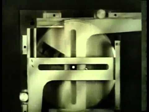
Providing uninterrupted, real-time fire control solutions requires the component solver—a precision mechanism that mechanically draws the vector diagram, resolves its right-angle components, and outputs those values as shaft rotations. The orientation of the speed vector is established by a vector gear containing a diametrical guide slot. The center line of the mechanism represents the optical line of sight to the target. When an input gear drives the vector gear, the angle of the slot rotates relative to the fixed center line, exactly reproducing the ship's heading relative to the line of sight.
To set the length of the vector, a spiral-grooved cam plate is mounted directly beneath the slotted vector gear and positioned by a dedicated speed input gear. A cam follower fitted with an upward-projecting pin rides in the spiral groove and passes through the slot of the vector gear above it, constraining the pin's travel strictly along the slot. When the ship's speed is zero, the spiral cam holds the pin precisely at the center axis of the gear. As higher speeds are introduced, the differential rotation between the cam and the slotted gear forces the pin outward along the slot. The narrator explains: “The distance from gear center to pin is the length of the speed vector.” At maximum rated speed, the pin reaches its extreme outward radius.
```mermaid flowchart LR accTitle: Component Solver Mechanism Flow accDescr: Mechanical inputs translate into physical rack displacements representing vector components. subgraph Inputs["Mechanical Inputs"] Course["Ship Course Input"] --> VG["Vector Gear Slot (Orientation)"] Speed["Ship Speed Input"] --> Cam["Spiral Cam (Radial Position)"] end subgraph Resolver["Pin & Crossed Slotted Racks"] VG & Cam --> Pin["Vector Pin (Position = Vector)"] Pin --> Rack1["Slotted Rack 1 (Range Rate)"] Pin --> Rack2["Slotted Rack 2 (Bearing Rate)"] end subgraph Outputs["Transmitted Quantities"] Rack1 --> OutRR["Range Rate Output Shaft"] Rack2 --> OutBR["Bearing Rate Output Shaft"] end ```
To decompose this physical vector into orthogonal components, the projecting pin extends upward through the intersecting slots of two perpendicular sliding racks: - **Range Rate Rack:** Slides parallel to the line of sight. As the pin tracks outward and turns, it pushes this rack an amount equal to the vector's projection along the line of sight. An output gear engaging the rack's teeth rotates proportionally, driving a shaft that delivers range rate to downstream computing elements. - **Bearing Rate Rack:** Constrained to slide perpendicularly to the line of sight, this rack measures the cross-line-of-sight component and rotates an independent output shaft representing bearing rate. - **Boundary Conditions:** When the ship steams directly down the line of sight, the bearing rate rack remains centered at zero displacement while the range rate rack displacement matches the full length of the speed vector; at zero speed, both racks remain centered at zero output.
[28:08](https://www.youtube.com/watch?v=s1i-dnAH9Y4&t=1688s) Continuous Integration and the Problem of Rangekeeping
Once rates of change are known, the computer must translate those rates into absolute position over time through integration. The film presents the disc-type integrator—one of several mechanical integrator designs used in naval fire control—and demonstrates its utility via rangekeeping. In basic rangekeeping against a stationary target where own ship steams along the line of sight, present range equals the algebraic sum of the initially measured range and the accumulated range change over time. If own ship closes the target, range change is negative and subtracts from initial range; if opening, it is positive and adds.
The narrator illustrates why manual or stepped arithmetic cannot handle this calculation: at a steady rate of 10 yards per second, range changes by 100 yards in 10 seconds, 200 yards in 20 seconds, and 300 yards in 30 seconds. In combat, however, range changes continuously rather than in ten-second leaps. Pointing out the failure of stepwise calculations, the narrator explains: “With ordinary arithmetic, you couldn't keep pace with this problem. And of more significance, the solution would be in a series of jumps. Range doesn't change this way. The integrator computes range change like this smoothly and continuously with the changing range.” The computed range change is fed directly into one input of a differential, while initial range is entered into the second input, yielding present range at the differential's output shaft.
- Present range is the algebraic sum of initial range and continuous range change. - Stepwise discrete calculation produces discontinuous "jumps" incompatible with fire control solutions. - The mechanical integrator generates a completely smooth, unbroken accumulation of range change across time.
[30:58](https://www.youtube.com/watch?v=s1i-dnAH9Y4&t=1858s) Anatomy and Operation of the Disc-Type Integrator
Lifting the cover off the physical disc integrator reveals its core operating assembly: a flat rotating disc, two precision steel balls held one above the other in a movable carriage, and an output roller resting atop the upper ball. Motion is governed by two distinct inputs. The first input is time, represented by the disc, which is driven by an electric motor at a rigorously constant rotational speed. The second input is range rate, supplied continuously by the component solver, which mechanically shifts the ball carriage radially across the face of the disc.
```mermaid flowchart TD accTitle: Disc Integrator Operating Chain accDescr: Motor and range rate inputs combine through frictional contact to produce range change. subgraph Inputs["Integrator Inputs"] Motor["Constant Speed Motor (Time: t)"] --> Disc["Rotating Disc"] RR["Range Rate Input (dr/dt)"] --> Carriage["Movable Ball Carriage (Radius: r)"] end subgraph Mechanism["Friction Drive"] Disc -->|"frictional drive"| Ball1["Lower Ball"] Ball1 --> Ball2["Upper Ball"] Carriage -.->|"sets radial position of"| Ball1 Ball2 -->|"drives"| Roller["Output Roller"] end subgraph Solution["Integration Output"] Roller --> Out["Revolutions = Accumulated Range Change"] Out --> Diff["Differential (+ Initial Range)"] Diff --> PR["Present Range"] end ```
Frictional contact between the spinning disc, the lower ball, the upper ball, and the roller drives the output shaft. The narrator compares this arrangement to an infinitely variable gear ratio: the circumferences of the roller and the intermediate idler balls remain fixed, but the circumferential track traced on the spinning disc varies according to how far the ball carriage is positioned from the disc center. Near the outer rim, the track circumference is large, causing the roller to spin at maximum speed. As the carriage is shifted inward, roller speed diminishes linearly until it reaches the exact center of the disc, where the disc track diameter is zero and roller rotation ceases entirely.
To illustrate the underlying mathematics: - Assume the disc turns at 1 revolution per second (displayed on a time counter). - Assume 1 revolution of the roller represents exactly 1 yard of range change (displayed on a range change counter). - An input range rate of 3 yards per second positions the ball carriage at a disc radius giving a 3:1 ratio, turning the roller at 3 revolutions per second and accumulating 3 yards each second.
Because range rates in tactical environments constantly fluctuate, the integrator treats the problem as an infinite series of instantaneous velocity increments, continuously integrating range rate with respect to time. Furthermore, the disc provides intrinsic algebraic sign handling. Positioning the balls on one side of center drives the roller forward (positive range rate, opening range), whereas shifting across center reverses the roller's direction (negative range rate, closing range). The narrator summarizes this operation: “Thus with any range rate high or low plus or minus the integrator continuously multiplies range rate by time and delivers range change which is the effective sum of all changes.”
[35:51](https://www.youtube.com/watch?v=s1i-dnAH9Y4&t=2151s) The Rack-Type Multiplier
The presentation transitions to mechanical multiplication, introducing devices engineered to compute the continuous product of two independent, continually varying inputs. As the narrator states: “Multipliers are mechanisms which can multiply two continuously changing values.” While different mechanical multiplier configurations exist, the film selects a rack-type multiplier to demonstrate the core geometric operating principles.
The assembly is built around two input racks, designated rack A and rack B, arranged at precise right angles to each other, alongside a designated output rack. Input rack A incorporates a slotted pivot arm that swings around a stationary base pin. Input rack B features its own longitudinal slot that links directly to the swinging pivot arm by means of a sliding connector termed the "multiplier pin." When either input rack shifts linearly in response to external data, it alters the angular attitude of the pivot arm and the position of the multiplier pin, beginning the geometric proportional linkage that yields the product of the two inputs.
[36:43](https://www.youtube.com/watch?v=s1i-dnAH9Y4&t=2203s) Operating the Mechanical Multiplier: Signed Values and Zero
The physical multiplier operates through a movable multiplier pin that engages directly with the slot of the output rack. As the two input racks shift their positions, they displace this pin and mechanically position the output rack. The baseline reference point occurs when the multiplier pin aligns perfectly with the stationary pin; at this exact alignment, both input racks and the output rack sit in their neutral zero positions. To clearly demonstrate the mathematical relationships at work, calibrated scales are positioned along each input rack and along the output rack, with positive values extending in one direction and negative values in the opposite direction.
The narrator walks through several arithmetic scenarios to illustrate how the linkage computes instantly across all quadrants. Setting an $A$ input of $+2$ alongside a $B$ input of $+3$ drives the output rack to exactly $+6$. Increasing both inputs to $+4$ pushes the output to $+16$. When the $A$ input remains fixed at $+4$ while the $B$ input drops to zero, the mechanism brings the output directly to zero. As the narrator emphasizes regarding null values, “When one input is zero, the output always is zero regardless of the other input value.”
The mechanism smoothly accommodates negative numbers without jamming or losing mechanical registration. Entering an input of $-3$ against $+4$ generates an output of $-12$, while pairing two negative inputs—such as $-2$ multiplied by $-4$—causes the mechanical geometry to invert signs properly, delivering an output of $+8$. The narrator highlights the elegance and speed of the hardware, observing, “It instantly delivers the product of any two input values even though the inputs are continuously changing.”
- **Input $A = +2$, Input $B = +3$**: Produces an output of $+6$. - **Input $A = +4$, Input $B = +4$**: Produces an output of $+16$. - **Input $A = +4$, Input $B = 0$**: Produces an output of $0$. - **Input $A = -3$, Input $B = +4$**: Produces an output of $-12$. - **Input $A = -2$, Input $B = -4$**: Produces an output of $+8$.
---
[39:38](https://www.youtube.com/watch?v=s1i-dnAH9Y4&t=2378s) Geometric Principles of the Multiplier: Similar Triangles and Scaling
The mathematical validity of the mechanism relies directly on Euclidean geometry. By establishing a baseline running through the stationary pin when the multiplier pin is centered over it, a fixed distance is measured along that line to the pivot pin. This baseline separation is designated as a constant, $K$. When input $A$ travels a distance $a$ and input $B$ travels a distance $b$, the resultant movement of the output rack is designated as distance $x$.
A line traced along the slot of the pivot arm cuts across these perpendicular displacements, creating two similar right-angled triangles whose corresponding sides remain strictly proportional. Because the ratio of the sides must match, the mathematical proportion is established as $x / b = a / K$. Multiplying both sides by the displacement $b$ yields the governing formula $x = (a \cdot b) / K$. As the narrator summarizes, “In other words, the output X equals the product of the two inputs divided by K, a constant.” Because distance $K$ is fixed for any given physical multiplier unit, its dividing effect is permanently normalized and compensated for through the gear ratios chosen for the input and output drives.
```mermaid flowchart LR accTitle: Geometric Multiplication via Similar Triangles accDescr: Diagram showing how inputs A and B relate through constant K to yield output X. subgraph Inputs ["Input Displacements"] A["Input A (Distance a)"] B["Input B (Distance b)"] end subgraph Geometry ["Similar Triangles Proportion"] Ratio["x / b = a / K"] KVal["Fixed Pivot Distance (K)"] end subgraph Output ["Mechanical Result"] X["Output x = (a * b) / K"] Gears["Output Gearing Compensates for 1/K"] end A --> Ratio B --> Ratio KVal --> Ratio Ratio --> X X --> Gears ```
- **Baseline Dimension ($K$)**: The fixed distance along the baseline between the stationary pin and the pivot pin. - **Similar Triangle Ratio**: Expressed geometrically as $x / b = a / K$. - **Output Formula**: Solved as $x = (a \cdot b) / K$, where the constant $1/K$ attenuation is eliminated by mechanical gear ratios.
---
[41:21](https://www.youtube.com/watch?v=s1i-dnAH9Y4&t=2481s) Series Conclusion: Modular Mechanisms in Fire Control Computing
The film concludes by reviewing the broader scope of the instructional series. Across the presentations, only seven fundamental computing mechanisms were introduced and analyzed. While the training spent only a modest amount of time examining each mechanism in isolation, this elemental breakdown provides the necessary conceptual foundation for understanding how physical hardware solves complex equations dynamically in naval warfare.
The narrator underscores the pedagogy behind mastering these components one by one, explaining: “Only seven mechanisms were described in parts one and two of this series and we have spent only a short time with each mechanism but it was enough to indicate how mechanisms are used for computing and how by studying the mechanisms separately you can gain much understanding of the instruments which solve the fire control problem.” Understanding these discrete components enables technicians and fire controlmen to comprehend the massive, interconnected electromechanical computers installed aboard naval combatants.
## Notable quotes > [00:00](https://www.youtube.com/watch?v=s1i-dnAH9Y4&t=0s) Obviously, computer accuracy depends on the quality of the information it receives and that depends on the skill and understanding of the men. — Narrator
> [19:42](https://www.youtube.com/watch?v=s1i-dnAH9Y4&t=1182s) Solving the fire control problem requires continuous information of the existing rates of change. — Narrator
## Mentioned Navy Ships, Excelsior10000
## Video description A 1953 training film for a mechanical fire control computer aboard Navy Ships. Amazing how problems of mathematical computation were solved so elegantly in "permanent" mechanical form, before microprocessors became inexpensive and commonplace.
[Source](https://www.youtube.com/watch?v=s1i-dnAH9Y4)