Dyalog APL Refactors Arthur Whitney's Solver to Crack 9x9 Sudoku

Dyalog

Precomputing the grid's contention map and passing it as an inner operand eliminates redundant calculations, allowing the breadth-first solver to resolve standard 9x9 puzzles instantly.

AI-assisted summary of A Sudoku Solver in APL — original source. Check the original for full context.

Source published: 2012-10-27

Key ideas

A Sudoku solver is constructed in APL based on an algorithm by Arthur Whitney, demonstrated incrementally starting with a 4×4 board before scaling to full 9×9 puzzles. (0:00)
Cell conflicts are modeled by joining row, column, and sub-box indices into coordinate triples, using outer product comparisons to generate a rank-4 boolean contention map (`cmap`). (1:17)
The solver employs a breadth-first search by identifying all empty cells (zeros) and folding a placement expansion function (`px`) over them across candidate board states. (6:33)
Precomputing the static contention map once at the top level and threading it down as an operand avoids thousands of redundant recalculations, enabling efficient solving of standard 9×9 puzzles. (8:01)

Detailed notes

## Background Published on YouTube by Dyalog on October 27, 2012, this video demonstrates the development of a Sudoku solver written in APL. Based on an algorithm by Arthur Whitney and presented by John Scholes, the description points viewers to experiment with the code at TryAPL.org and consult notes on the breadth-first search implementation.

## TL;DR The video walks through constructing an elegant Sudoku solver from first principles in APL, initially modeling the logic on a 4×4 grid before scaling to a standard 9×9 board. It establishes cell coordinates across rows, columns, and sub-boxes, then generates a boolean contention map to identify valid candidate numbers for any empty cell. By designing placement operators and folding them across the list of blank cells, the solver executes a breadth-first search to branch all legal boards until reaching a solution. Finally, the implementation is optimized by hoisting the repeated contention map calculation into a single precomputed operand passed down the call chain, allowing full 9×9 puzzles to be solved instantly.

## Atmosphere & style The presentation carries the calm, deliberate, and mesmerizing precision characteristic of classic APL demonstrations. John Scholes guides the viewer step by step through dense mathematical abstractions with a quiet, measured cadence, transforming complex array transformations into seemingly effortless one-liners. Watching it feels like observing a master craftsman at a digital workbench—intense, highly cerebral, and deeply satisfying as intricate grid logic crystallizes into a handful of glyphs.

## Bulletin - [00:00](https://www.youtube.com/watch?v=DmT80OseAGs&t=0s) A Sudoku solver is constructed in APL based on an algorithm by Arthur Whitney, demonstrated incrementally starting with a 4×4 board before scaling to full 9×9 puzzles. - [01:17](https://www.youtube.com/watch?v=DmT80OseAGs&t=77s) Cell conflicts are modeled by joining row, column, and sub-box indices into coordinate triples, using outer product comparisons to generate a rank-4 boolean contention map (`cmap`). - [06:33](https://www.youtube.com/watch?v=DmT80OseAGs&t=393s) The solver employs a breadth-first search by identifying all empty cells (zeros) and folding a placement expansion function (`px`) over them across candidate board states. - [08:01](https://www.youtube.com/watch?v=DmT80OseAGs&t=481s) Precomputing the static contention map once at the top level and threading it down as an operand avoids thousands of redundant recalculations, enabling efficient solving of standard 9×9 puzzles.

## Key takeaways - [00:00](https://www.youtube.com/watch?v=DmT80OseAGs&t=0s) Sudoku grid geometry is generalized using sub-box dimensions of 2 for a 4×4 board and 3 for a 9×9 board. - [00:00](https://www.youtube.com/watch?v=DmT80OseAGs&t=0s) Each cell on the board is represented by a coordinate triple comprising its row, column, and sub-box index. - [00:00](https://www.youtube.com/watch?v=DmT80OseAGs&t=0s) A helper function named `box` generates sub-grid identifiers by shaping indices and replicating elements across rows and columns. - [01:17](https://www.youtube.com/watch?v=DmT80OseAGs&t=77s) Contention between cells occurs whenever two cells share the same row, column, or sub-box index. - [01:17](https://www.youtube.com/watch?v=DmT80OseAGs&t=77s) An outer product comparison across all coordinate triples yields a rank-4 array that encloses into a grid of boolean contention masks (`cmap`). - [01:17](https://www.youtube.com/watch?v=DmT80OseAGs&t=77s) Candidate digits for any cell are determined by applying its contention mask to the puzzle and subtracting conflicting numbers from the universe of valid digits. - [01:17](https://www.youtube.com/watch?v=DmT80OseAGs&t=77s) Empty cells are identified by testing the puzzle matrix for zero values. - [02:47](https://www.youtube.com/watch?v=DmT80OseAGs&t=167s) A placement operator uses double-alpha (`⍺⍺`) addressing to insert digits into specific cell coordinates without altering the rest of the board. - [02:47](https://www.youtube.com/watch?v=DmT80OseAGs&t=167s) The function `pvec` generates a vector of next-state boards corresponding to each valid candidate digit for a target cell. - [06:33](https://www.youtube.com/watch?v=DmT80OseAGs&t=393s) Filtering indexed puzzle coordinates with the zero mask produces an ordered vector of all empty cell coordinates needing assignment. - [06:33](https://www.youtube.com/watch?v=DmT80OseAGs&t=393s) Folding the placement operator `px` over all empty cells executes a breadth-first search across all legal board completions. - [08:01](https://www.youtube.com/watch?v=DmT80OseAGs&t=481s) The initial naive implementation suffered from severe performance degradation because `cmap` was recomputed on every candidate check within the search tree. - [08:01](https://www.youtube.com/watch?v=DmT80OseAGs&t=481s) Refactoring the solver to compute `cmap` once at the top level and pass it through operators via operand syntax (`⍺⍺`) eliminates redundant recalculations. - [08:01](https://www.youtube.com/watch?v=DmT80OseAGs&t=481s) With the contention map precomputed, the concise APL solver scales directly to solve standard 9×9 Sudoku puzzles.

## Detailed walkthrough ### [00:00](https://www.youtube.com/watch?v=DmT80OseAGs&t=0s) Building Box Numbers and Row-Column-Box Coordinates

The construction of the Sudoku solver begins by formulating how grid coordinates and sub-grid "box" regions are identified. To demonstrate the mathematics cleanly before tackling a standard 9×9 grid, operations are demonstrated on a smaller 4×4 Sudoku puzzle. In a 9×9 grid, the boxes are 3×3, while in a 4×4 puzzle, the sub-boxes are 2×2. The narrator starts by defining a function to generate box indices using the indices of a 3-element vector, shaping omega to the power of two, reshaping into a 3-row, 3-column matrix, and replicating items across both rows and columns. This yields a helper named `box` that calculates the sub-grid box numbers for any cell.

To establish the coordinates across the board, the row and column indices of the 4×4 array are paired, and each cell coordinate is joined with its corresponding box number. Here, `box` computes the region identifier by taking the square root of the first item of omega (`Omega to the power a half`). Applying this across the entire grid produces a 3-element descriptor—row, column, and box number—for every individual cell in the puzzle.

```mermaid flowchart LR accTitle: Cell Coordinate Construction accDescr: Process of building row, column, and box coordinate triples for a Sudoku grid. subgraph Grid Setup A["Grid Dimensions"] --> B["Row & Column Indices"] A --> C["Sub-box Partitioning"] end subgraph Coordinate Assembly B --> D["Cell Coordinate Triple (Row, Col, Box)"] C --> D end ```

- In a 9×9 puzzle, the sub-box dimension is 3, whereas in a 4×4 puzzle, the sub-box dimension is 2. - The coordinate structure associates each cell with a 3-tuple `(Row, Column, Box)`.

---

[01:17](https://www.youtube.com/watch?v=DmT80OseAGs&t=77s) Calculating the Contention Map and Available Digits

With every cell indexed by its row, column, and box numbers, the next step is determining cell contention. Two cells cannot share the same value if they sit in the same row, column, or box. Comparing an individual cell's coordinate triple (such as `3 3 4`) itemwise with other cells reveals a conflict: “There is contention where one is a member of each cell.” By extending this logic across the entire board using an outer product comparison across all cells, the system produces a rank-4 array. Enclosing the first two axes reduces this structure to a 4×4 map containing 4×4 boolean contention matrices. This function is named `cmap` (contention map).

To demonstrate how the contention map operates, an example 4×4 puzzle is loaded with blank squares represented by zeros. Selecting a specific cell, such as the third row and second column (cell `3 2`), retrieves its corresponding contention mask. When this boolean mask is applied back to the puzzle, it extracts all numbers currently occupying the same row, column, or 2×2 box as that cell. Subtracting these conflicting values from the set of all possible numbers (1 to 4 for a 4×4 board) isolates the exact candidate numbers available to be legally placed into that cell.

- A cell conflicts with any other cell sharing an identical row, column, or box index. - Outer product comparison produces a rank-4 array, which encloses to a 4×4 grid of boolean contention masks. - Zeros represent empty squares in the board representations.

---

[02:47](https://www.youtube.com/watch?v=DmT80OseAGs&t=167s) Placing Digits and Generating Candidate Placements

Building on the candidate finder, the algorithm develops an operator to place a chosen candidate digit into a target cell. Using left and right operands, an inner operand receives the target coordinates (such as `3 2`), addressed via double-alpha (`⍺⍺`). Using a take operation based on puzzle dimensions combined with an additive assignment mask, the operator places a value into the board array without disturbing the remaining cells. For instance, testing the operator allows placing a value like `99` directly at cell `(1, 1)`.

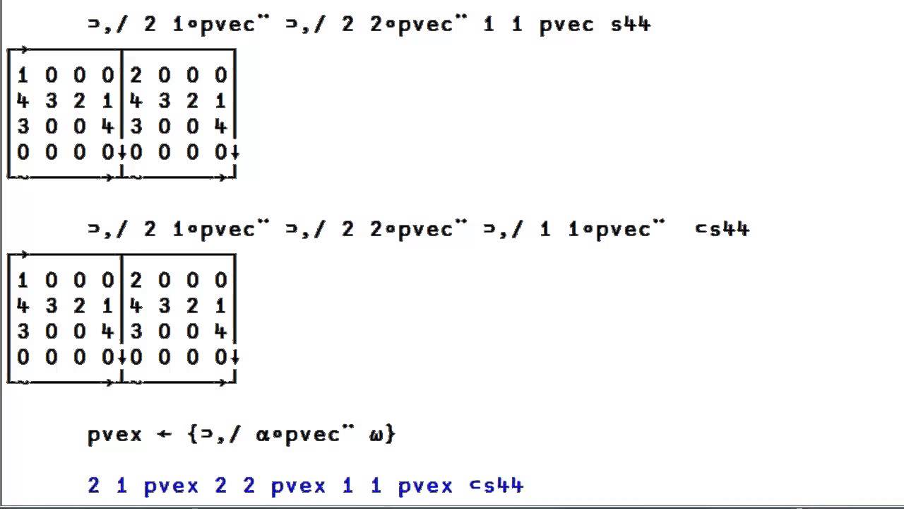
To advance board states during solving, the solver needs to generate all valid next-state boards for a specific cell. Given an empty cell at coordinates `(1, 1)`, the candidate function identifies which numbers can legally be played there. The placement function `pvec` is then mapped over each available candidate number, generating a vector of updated boards—one board for every candidate choice. Similarly, binding coordinates `(2, 2)` produces a series of board placements for that cell. This logic is abstracted into functions that take a cell coordinate, evaluate valid digits, and output the resulting list of populated board states.

- Target cell insertion is parameterized as an operator using double-alpha (`⍺⍺`) addressing. - Function `pvec` generates a vector of updated board configurations corresponding to each candidate digit for a single cell.

---

[06:33](https://www.youtube.com/watch?v=DmT80OseAGs&t=393s) Finding Empty Cells and Folding Over Placements

To systematically solve the whole puzzle, the solver must locate all unsolved cells and iteratively test valid placements across them. By inspecting the puzzle matrix, a boolean mask identifies all locations containing zeros. Multiplying this mask against the grid index matrix and filtering out zero entries isolates a vector containing the coordinates of every blank cell in the puzzle.

With the blank cells identified, the solver applies a reduction fold. A higher-order function, `px`, maps candidate placements for a cell across an entire list of candidate boards, expanding each current partial board into multiple new possibilities. Starting with the original unfilled board, folding `px` over the list of empty cells systematically branches through the possibilities: “Using all of the empty cells we have a solution vector for the puzzle s44.” For the sample 4×4 puzzle, this reduction succeeds in producing the completed solution vector.

```mermaid flowchart TD accTitle: Sudoku Breadth-First Expansion Flow accDescr: Flowchart showing how empty cells are extracted and folded over placements to generate solutions. subgraph Discovery A["Puzzle Matrix"] --> B["Detect Zero Cells"] B --> C["Vector of Empty Cell Coordinates"] end subgraph Expansion C --> D["Fold Placement Operator (px)"] D --> E["Branch Candidate Boards"] E --> F["Solution Vector"] end ```

- Blank cells are discovered by matching zero entries and compressing the index vector. - Folding the placement expansion over every empty cell performs a breadth-first search across all legal board completions.

---

[08:01](https://www.youtube.com/watch?v=DmT80OseAGs&t=481s) Optimizing Performance and Solving a 9x9 Sudoku

While the initial implementation correctly solves the 4×4 puzzle, the narrator highlights a significant architectural flaw: “However this coding is inefficient.” When `svec` folds `px` across empty cells, `px` calls `pvec` for every placement, `pvec` calls `avl` for every available number, and `avl` recalculates the exact same contention map (`cmap`) from scratch on every single invocation. Because the board geometry and cell relationships never change during the solve, recomputing the contention map thousands of times creates massive redundant overhead.

To fix this bottleneck, the code is refactored so that `svec` calculates `cmap` exactly once at the top level. The precomputed map is then passed down as an inner operand (`⍺⍺`) into `px`, forwarded as an inner operand (`⍺⍺`) into `pvec`, and finally received as `⍺⍺` inside `avl`. With this optimization in place, the algorithm avoids repeated grid analysis while retaining identical logic. The narrator applies the refined solver to a full 9×9 Sudoku puzzle, immediately producing the resolved grid. The presentation closes by displaying the concise, final APL code and encouraging viewers: “Try it for yourself at www.TryAPL.org.”

- Redundant calculation of `cmap` inside `avl` causes severe performance degradation during board search. - Precomputing `cmap` once in `svec` and passing it down via the operand syntax (`⍺⍺`) eliminates redundant work. - The completed solver operates seamlessly on standard 9×9 puzzles using Arthur Whitney's breadth-first search formulation.

## Mentioned APL, Arthur Whitney, Dyalog, Dyalog APL, John Scholes, Sudoku, The APL Challenge, The APL Forge, TryAPL.org

## Video description Development of a Sudoku solver in APL. You might want to hit pause now and again. Experiment for yourself at http://www.TryAPL.org. Notes on the algorithm: http://dfns.dyalog.com/n_sudoku_bfs.htm

Algorithm: Arthur Whitney Performance: John Scholes

--------------------

GET STARTED

Download the latest version of Dyalog: https://www.dyalog.com/downloads

TAKE PART IN OUR APL COMPETITIONS

THE APL CHALLENGE Learn APL and compete for one of three $100 prizes. Open to all experience levels. https://challenge.dyalog.com

THE APL FORGE Got a problem to solve or a library to share? Use Dyalog APL to build something great — and win £2,500 + an expenses-paid trip to present at a Dyalog user meeting. https://forge.dyalog.com

--------------------

[Source](https://www.youtube.com/watch?v=DmT80OseAGs)

中文简报

Dyalog APL重构Arthur Whitney求解器以破解9x9数独预先计算网格冲突图并将其作为内部操作数传递，消除了冗余计算，使广度优先求解器能够瞬间解出标准9x9数独谜题。该视频演示了如何在APL中从第一性原理构建一个优雅的数独求解器，最初在4×4网格上进行逻辑建模，随后扩展到标准9×9棋盘。它建立了跨行、列和小九宫格的单元格坐标，接着生成布尔冲突图以识别任意空格的有效候选数字。通过设计填数算子并将其折叠应用于空格列表，求解器执行广度优先搜索来分支所有合法棋盘，直至得出解决方案。最后，该实现通过将重复的冲突图计算提升为单个预先计算的操作数并沿调用链向下传递来完成优化，使得标准9×9谜题能够被瞬间解出。基于Arthur Whitney的算法在APL中构建了一个数独求解器，并以4×4棋盘为起点进行渐进式演示，随后扩展至完整9×9谜题。 (0:00) 通过将行、列和小九宫格索引合并为坐标三元组，并利用外积比较生成4阶布尔冲突图（`cmap`），以此对单元格冲突进行建模。 (1:17) 求解器采用广度优先搜索，通过识别所有空格（零值）并在候选棋盘状态中对其折叠应用填数扩展函数（`px`）。 (6:33) 在顶层预先计算一次静态冲突图并将其作为操作数向下传递，避免了数千次冗余重新计算，从而能够高效求解标准9×9谜题。 (8:01)

Reading summary

Dyalog presents an array-oriented Sudoku solver in APL that models board constraints geometrically and resolves puzzles via breadth-first reduction folding. The algorithm models grid conflict rules as boolean contention masks, dynamically generates candidate boards, and relies on operand passing to eliminate redundant computations. Grid Geometry and Boolean Contention Mapping (0:00) The solver models puzzle cells as coordinate triples containing a row index, a column index, and a sub-box identifier. For a 4×4 board, sub-boxes are 2×2, while a standard 9×9 grid uses 3×3 regions. The helper function box computes these sub-grid identifiers by taking the square root of the board dimension and replicating the resulting indices across rows and columns. Pairing row and column coordinates with their box numbers creates a distinct 3-tuple descriptor for every cell on the board. Contention between cells occurs whenever two positions share a row, column, or box index. By executing an itemwise outer product comparison across all cell descriptors, the program generates a rank-4 array that is enclosed into a grid of boolean contention masks named cmap. Applying an empty cell's mask to the board isolates all existing numbers in its row, column, and box. Subtracting those values from the set of all possible digits leaves the legal candidate values for that position. Candidate Placement and State Generation (2:47) Placing candidate numbers into target cells is implemented through an operator that receives target coordinates as an inner operand via double-alpha (⍺⍺) syntax. By combining grid-dimension take operations with an additive assignment mask, the operator inserts a digit into the specified coordinate without modifying any neighboring cells. To advance the puzzle state, the function pvec couples candidate lookup with placement execution. Given an empty cell coordinate, it retrieves all valid digits and maps the placement operator over each candidate value. This generates a vector of updated board configurations representing every legal single-cell branch from the current board. Breadth-First Solving via Reduction Folding (6:33) To process the entire board, the solver identifies unsolved squares by matching zero entries in the puzzle matrix. Compressing the grid index matrix against this zero mask produces a coordinate vector containing every blank cell that must be solved. The algorithm then uses a reduction fold to conduct a breadth-first search across all board states. The higher-order function px expands an existing list of candidate boards by mapping pvec over an empty cell's coordinates. Beginning with the initial partially filled board, folding px across the vector of blank coordinates systematically evaluates every branch, returning a vector of fully completed solutions. Performance Optimization via Operand Passing (8:01) Although functionally correct on sample 4×4 puzzles, the initial solver contained an architectural bottleneck: each evaluation of available digits recomputed the identical cmap contention map from scratch. Because the board's geometric constraints never change during search, repeating these calculations across thousands of search branches introduced significant redundant overhead. The implementation was refactored so that the top-level solving function computes cmap only once. The precalculated map is subsequently passed down as an inner operand (⍺⍺) through px, forwarded to pvec, and consumed by the candidate function. Eliminating repeated contention calculations enables Arthur Whitney's breadth-first formulation to execute efficiently on standard 9×9 Sudoku puzzles. The presentation highlights that expressive array operations can concisely solve combinatorial search problems, though practical performance hinges on avoiding repetitive geometry recalculations by passing immutable board structures down the call chain.

精炼阅读摘要

Dyalog 演示了基于 Arthur Whitney 算法架构的 APL 数独求解器实现，通过外积冲突映射与广度优先折叠搜索解决数独谜题。坐标结构与冲突掩码构建 (0:00) 求解器的数学建模首先建立网格单元的坐标标识体系。在标准 9×9 盘面中子宫格维度为 3×3，而在示例的 4×4 盘面中子宫格为 2×2。程序通过对维度开平方等数组变换生成区域编号，将每个单元格编码为包含行号、列号与子宫格号的三元组描述符。在数独规则中，凡处于相同行、列或宫格的两个单元格均存在数值互斥。系统借助外积比较全盘单元格的三元组信息，生成一个 4 阶数组，随后闭合前两个轴得到由布尔掩码构成的冲突图（cmap）。空单元格在盘面中以数字 0 占位。针对指定单元格提取其布尔冲突掩码并映射至当前盘面，即可过滤出同行、同列和同宫已出现的数字；从候选全集中剔除这些冲突数值后，便能准确确定该单元格的合法可填数字集。候选展开与广度优先分支搜索 (2:47) 在确定合法数字后，求解器构建算子将候选值填入目标坐标。算法利用左操作数与右操作数机制，通过双阿尔法（⍺⍺）语法绑定单元格坐标，结合盘面尺寸截取与加法赋值掩码完成填值而不破坏其他单元格状态。函数 pvec 针对目标单元格的每个有效候选数字分别生成更新后的盘面向量。全盘求解流程依赖对未填单元格的系统化搜寻。通过比对盘面矩阵中的 0 并压缩坐标矩阵，程序提取出全部待解空格坐标向量。高阶函数 px 进而将特定单元格的填值操作映射至整个候选盘面列表。以初始残局为起点，将 px 沿空格坐标列表进行折叠归约（fold reduction），算法以广度优先搜索的方式逐级展开分支，最终在 4×4 示例中求得完整的解向量。预计算优化与 9x9 盘面求解 (8:01) 演讲者指出初始实现存在显著的性能缺陷。在展开折叠过程中，外层函数逐步调用 px、pvec 与候选求解函数 avl，导致每次查询有效数字时均会重复从头计算冲突图 cmap。由于盘面的几何结构与单元格互斥关系在求解期间完全固定，成千上万次的重复运算带来了巨大的无谓开销。为消除性能瓶颈，代码经过重构由顶层函数 svec 一次性预先计算 cmap，再通过操作数语法（⍺⍺）层层向下传递至 px、pvec 以及底层的 avl。此项优化避免了冗余的几何分析并保留了纯粹的数组逻辑，使算法能够无缝扩展并即时求解标准的 9×9 完整数独题目。该程序展示了使用 APL 数组范式实现数独求解的简洁性，但其效率高度依赖顶层冲突图的预计算与操作数传递；演讲者建议读者在 TryAPL 在线平台测试该实现。

Detailed notes — zh

## Background 本视频由 Dyalog 于 2012 年 10 月 27 日发布在 YouTube 平台。视频简介说明该内容展示了使用 APL 语言开发数独求解器的过程，算法基于 Arthur Whitney 的设计并由 John Scholes 进行演示，同时鼓励观众在 TryAPL 网站上亲自动手实验。 ## TL;DR 视频首先通过行、列及宫（RCB）的三元几何结构，借助外积计算构建出数独盘面的冲突映射矩阵（cmap）。接着，演示了利用冲突掩码提取可用候选数字（avl），并结合数组重塑编写放置算子以生成衍生盘面分支（pvec）。随后，程序将所有空格坐标组成向量，使用规约折叠（fold / reduction）机制驱动广度优先搜索，自动淘汰无效分支并得出解答。最后，针对嵌套调用中重复计算冲突矩阵的性能瓶颈，通过将不变的几何结构提升至顶层并作为操作数透传重构代码，实现了能瞬间求解 9x9 标准数独的高性能简洁求解器。 ## Atmosphere & style 整个演示风格极其严谨、凝练而富有极客美感，没有多余的废话，完全以纯粹的代码推演和数据流变换为主导。解说语调沉着冷静，一步步将看似复杂的数独规则拆解为纯粹的高阶张量运算与折叠操作，展现出一种数学式的工整与优雅。随着逻辑从 4x4 玩具模型平滑推导至规约搜索，再到最后直面性能瓶颈进行精准重构，观众能直观感受到 APL 语言那种以极少字符迸发强大表达力的震撼与智力愉悦感。 ## Bulletin - [00:00](https://www.youtube.com/watch?v=DmT80OseAGs&t=0s) 本演示基于 Arthur Whitney 的广度优先搜索算法与 John Scholes 的实现，展示了如何在 APL 中纯函数式地构建数独求解器。 - [00:00](https://www.youtube.com/watch?v=DmT80OseAGs&t=0s) 算法利用数组外积将行、列、宫的三元属性（RCB）快速比对，为网格生成全局冲突映射矩阵（cmap）。 - [05:04](https://www.youtube.com/watch?v=DmT80OseAGs&t=304s) 求解核心将全部空格坐标与初始盘面结合，利用规约运算符（reduction / fold）从右向左逐级展开可能盘面，自然过滤掉无效分支。 - [08:01](https://www.youtube.com/watch?v=DmT80OseAGs&t=481s) 针对几何结构重复计算的性能瓶颈，通过将不变的冲突映射表作为操作数在顶层提升并向下透传，使 9x9 数独难题得以瞬间求解。 ## Key takeaways - [00:00](https://www.youtube.com/watch?v=DmT80OseAGs&t=0s) 使用向量索引、矩阵重塑与行列项复制构建 box 函数，用于快速计算数独中各单元格所属的宫编号。 - [00:40](https://www.youtube.com/watch?v=DmT80OseAGs&t=40s) 为单元格建立行、列、宫（RCB）三元属性，并通过开方操作适配不同规模的数独网格（如 4x4 与 9x9）。 - [01:25](https://www.youtube.com/watch?v=DmT80OseAGs&t=85s) 利用外积（outer product）对整个网格的 RCB 三元组进行逐项比较，只要行列宫有重合即判定为冲突，形成四阶布尔张量。 - [01:55](https://www.youtube.com/watch?v=DmT80OseAGs&t=115s) 沿前两个轴对冲突张量执行封闭（enclose），构建出每个单元格对应一张冲突掩码的映射矩阵 cmap。 - [02:17](https://www.youtube.com/watch?v=DmT80OseAGs&t=137s) 通过单元格坐标检索 cmap 掩码并与当前盘面相乘，结合差集运算从全集数字中剔除既有冲突值，即可算出可用候选数（avl）。 - [03:02](https://www.youtube.com/watch?v=DmT80OseAGs&t=182s) 定义双重 alpha 参数（⍺⍺）的位置放置算子，利用负索引截取与重塑技术将候选数字填入盘面指定位置。 - [04:00](https://www.youtube.com/watch?v=DmT80OseAGs&t=240s) 将 avl 计算出的候选数字映射至放置算子，生成可为单个空格衍生所有合法后续状态的放置向量（pvec）。 - [05:04](https://www.youtube.com/watch?v=DmT80OseAGs&t=304s) 提取盘面中所有值为 0 的单元格坐标，构成待填空格索引向量，作为状态展开的驱动序列。 - [06:00](https://www.youtube.com/watch?v=DmT80OseAGs&t=360s) 借助 APL 的规约运算符（fold /），将放置展开函数 px 沿空格坐标向量从右向左折叠，驱动广度优先搜索（BFS）层层派生分支。 - [07:10](https://www.youtube.com/watch?v=DmT80OseAGs&t=430s) 非法分支在多步迭代中因无法产生可用数字而自然夭折，遍历完全部空格后最终保留下来的即为合法解向量。 - [08:01](https://www.youtube.com/watch?v=DmT80OseAGs&t=481s) 初始实现中每个分支递归都会重复重新计算恒定的 cmap 几何结构，构成了严重的算力浪费和性能瓶颈。 - [08:30](https://www.youtube.com/watch?v=DmT80OseAGs&t=510s) 性能优化的核心是将不变的 cmap 计算提升（hoist）至顶层求解函数中，单次计算后作为内操作数（⍺⍺）向下逐层静态注入。 - [09:05](https://www.youtube.com/watch?v=DmT80OseAGs&t=545s) 经过操作数透传优化后，代码保持了相同的函数式语义，但消除了冗余高维计算，可瞬间求解 9x9 标准数独难题。 ## Detailed walkthrough ### [00:00](https://www.youtube.com/watch?v=DmT80OseAGs&t=0s) 构建数独宫格编号与冲突映射矩阵（Contention Map）演示从构建数独的几何结构开始。首先利用 3 向量索引构建函数，生成 $\omega^2$（即 $3^2=9$）的索引，再通过重塑（reshape）为 3 行 3 列的数字矩阵，结合行项复制（row item replication）和列项复制（column item replication），由此构造出名为 `box` 的函数，用于计算 $9 \times 9$ 数独谜题中各个单元格所属的宫编号（box number）。为了便于直观演示与理解，讲解转向一个更轻量级的 $4 \times 4$ 数独谜题。在 $4 \times 4$ 的场景中，系统的核心是为每个单元格赋予一组由“行索引、列索引、宫编号”构成的三元属性（Row-Column-Box, 简称 RCB）。通过对数组形状开方（$\omega^{0.5}$）并与行列索引拼接，每个单元格均生成对应的行、列、宫标记。接着，系统通过外积（outer product）对整个网格进行单元格间的三元组逐项比对：只要两个单元格在行、列或宫三者中有任意一项相同（即数值重合、存在包含关系），即判定它们之间存在冲突（contention）。对所得的四阶数组沿着前两个轴进行封闭（enclose），便生成了一个 $4 \times 4$ 的冲突映射矩阵，记为 `cmap`。每一个单元格位置都对应一张 $4 \times 4$ 的布尔冲突掩码（contention mask）。 ```mermaid flowchart LR accTitle: Contention Map Generation accDescr: Diagram illustrating how row, column, and box indices are processed into a contention map. subgraph S1["几何属性构建"] A["4x4 网格"] --> B["行/列索引"] A --> C["计算宫编号 (box)"] B & C --> D["RCB 组合三元组"] end subgraph S2["冲突矩阵计算"] D --> E["外积逐项比较<|cell_split|>outer product"] E --> F["高维数组封闭 (enclose)"] F --> G["冲突映射表 (cmap)"] end ``` ### [02:17](https://www.youtube.com/watch?v=DmT80OseAGs&t=137s) 查找可用数字与位置放置算子（Placement Operator）讲解引入了一个带空格的 $4 \times 4$ 数独矩阵（变量记为 `s44`），其中用数字 `0` 代表空白格子。通过查询该谜题的 `cmap`，可以精准提取指定单元格的冲突掩码。例如，选择第 3 行第 2 列（`3 2`）的单元格，提取该位置的掩码后，与数独当前盘面相乘筛选，即可得到与该格子处于同一行、同一列或同一宫的所有既有冲突数字。从全集数字 $1 \sim 4$ 中扣除这些冲突数字后，剩下的就是该单元格所有允许填入的可用数字（available numbers, 记为 `avl` 函数）。紧接着，讲解实现了一个放置算子（placement operator），用以将候选数值填入盘面的指定位置。该算子使用双重 $\alpha$（`⍺⍺`）接收单元格坐标（如 `3 2`），并利用负索引取值（negative take）与数组重塑技术，将新数值注入到原谜题数组中。例如，将数字 `99` 放入 `s44` 的 `1 1` 位置。将 `avl` 算出的可用候选数字与该放置算子结合，即可生成一个“放置向量”（placement vector, 记为 `pvec`）——它能为指定空格衍生出所有可能合法的后续盘面状态。 - “这里是一个用 0 表示空格的 4x4 数独谜题”：“here is a 4x4 Sudoko puzzle with zeros representing blank squares”。 - 空格可用数字计算逻辑：以目标单元格为索引查询 `cmap` 得到冲突掩码，提取盘面上对应的非零数字集合，再由全集向量做差集过滤（without the contention numbers）。 ### [05:04](https://www.youtube.com/watch?v=DmT80OseAGs&t=304s) 递归分支扩展与空格向量（Fold 与 Reduction）有了针对单个单元格生成后续盘面的机制后，下一步是将其串联以处理多个空格。如果对单元格 `(1, 1)` 执行放置向量生成，会得到若干新的中间盘面；对每一个新盘面，再针对下一个空位（例如 `(2, 2)` 或 `(2, 1)`）继续应用放置函数。通过右结合段的合理归纳（rationalizing the rightmost segment），这一连锁衍生过程被高度抽象为放置向量展开函数（`px`）。随后，讲解展示了 APL 极具表现力的一面：将一组待填空格坐标向量与初始谜题组合，通过规约（reduction / fold，即 `/`）运算符，从右向左依次应用 `px` 展开： - 提取谜题矩阵中数值为 `0` 的元素坐标，形成空白单元格索引向量。 - 将全部空白坐标组成向量，使用规约运算一次性对初始盘面进行广度优先分支迭代（BFS）。 - 当规约遍历完所有空格后，无效的分支自然死绝，最终直接输出了包含正确解的解答向量（solution vector）。 ```mermaid flowchart TD accTitle: Sudoku Solving Process via Fold accDescr: Pipeline of identifying empty cells and folding the placement expansion operator. A["输入盘面 s44"] --> B["筛选值为 0 的单元格"] B --> C["生成待填空格坐标向量"] C & A --> D["对空格向量执行规约 (fold /)"] subgraph BFS["广度优先分支搜索 (px / pvec)"] D --> E["为空格计算 avl 候选数"] E --> F["利用 placement 算子生成衍生分支盘面"] F --> G["对下一个空格继续映射展开"] end G --> H["输出解向量 (solution vector)"] ``` ### [08:01](https://www.youtube.com/watch?v=DmT80OseAGs&t=481s) 性能优化与 9x9 完整求解器呈现尽管上述纯函数式写法逻辑优美，但实现中存在严重的重复开销。讲述者明确指出了其效率瓶颈：“然而这种编码方式效率低下”：“however this coding is inefficient”。其深层原因在于调用链路：`svec` 将 `px` 折叠到所有空单元格上，`px` 对每个盘面状态调用 `pvec`，`pvec` 对每个可用数字调用 `avl`，而 `avl` 每次都在重复计算完全相同的 `cmap RCB`。由于数独的几何行列宫结构在整个求解过程中是恒定不变的，每次候选数检索都重新计算一次高维冲突图，造成了海量的算力浪费。为了彻底消除冗余计算，程序进行了关键性能重构： 1. 在顶层求解函数 `svec` 中，仅执行一次 `cmap RCB ⍴⍵` 计算。 2. 将计算好的冲突表作为左内操作数（inner operand `⍺⍺`）向下透传给 `pvec`。 3. `pvec` 再将其作为内操作数传递给 `avl`，由 `avl` 直接作为 `⍺⍺` 接收并消费。经过这层重构，算法保持了相同的逻辑语义，但执行效率大幅跃升。视频随后输入了一个完整的 $9 \times 9$ 标准数独难题，运行重构后的求解函数，瞬间输出解答向量。最后屏幕给出了最终优雅、凝练的完整 APL 代码，并提示观众可以前往 TryAPL 在线环境自行动手实验。 - 嵌套调用链关系：`svec` 规约折叠 `px` $\rightarrow$ `px` 遍历调用 `pvec` $\rightarrow$ `pvec` 遍历可用数调用 `avl` $\rightarrow$ `avl` 查询冲突掩码。 - 优化核心手段：计算提升（hoisting），将不变量从深层递归中移出，改由操作数（operands）机制逐级静态注入。 - 视频结尾邀请用户体验：“在 www.TryAPL.org 亲自动手试试吧”：“try it for yourself at www.TryAPL.org”。 ## Mentioned APL, Dyalog APL, Arthur Whitney, John Scholes, TryAPL ## Video description Development of a Sudoku solver in APL. You might want to hit pause now and again. Experiment for yourself at http://www.TryAPL.org. Notes on the algorithm: http://dfns.dyalog.com/n_sudoku_bfs.htm Algorithm: Arthur Whitney Performance: John Scholes -------------------- GET STARTED Download the latest version of Dyalog: https://www.dyalog.com/downloads TAKE PART IN OUR APL COMPETITIONS THE APL CHALLENGE Learn APL and compete for one of three $100 prizes. Open to all experience levels. https://challenge.dyalog.com THE APL FORGE Got a problem to solve or a library to share? Use Dyalog APL to build something great — and win £2,500 + an expenses-paid trip to present at a Dyalog user meeting. https://forge.dyalog.com -------------------- [Source](https://www.youtube.com/watch?v=DmT80OseAGs)

Original transcript

[0:00] the indices of a three [0:03] Vector a function for the indices of [0:05] Omega to the^ 2 where Omega is [0:09] three the three row three column reshape [0:13] of the [0:14] numbers the three row item [0:17] replication and a three column item [0:24] replication box denotes a [0:27] function for the Box numbers [0:31] of a 9x9 Sudoku puzzle we'll start with [0:34] a smaller 4x4 [0:38] puzzle the row column [0:41] indices of a 4x4 [0:47] array the join of each cell with its box [0:52] number where box takes the first item of [0:56] Omega to the power a half [1:04] row column box [1:05] numbers for each [1:08] cell row column box numbers for a 4x4 [1:17] puzzle itemwise [1:19] comparison with a cell containing [1:24] 334 there is contention where one is a [1:27] member of each cell [1:34] the outer product comparison with all [1:42] cells is a rank four [1:46] array enclosing the first two [1:51] axes the shape of the [1:57] shape produces a 4x4 map of 4x4 [2:01] contention [2:03] matrices C [2:06] map denotes a function for the [2:09] contention [2:10] map here's a contention [2:14] map for a 4x4 [2:17] puzzle here is a 4x4 Sudoko puzzle with [2:20] zeros representing blank [2:24] squares the shape of the [2:28] puzzle a contention [2:30] map for the [2:32] puzzle the third row second column left [2:37] argument cell [2:41] selection the cell item is the [2:44] contention [2:47] mask the puzzle [2:52] again numbers in contention with a cell [2:55] at 32 [3:01] all numbers 1 to [3:03] four without the contention [3:09] numbers numbers [3:14] available to cell [3:16] one1 in puzzle [3:25] s44 left and right function arguments [3:31] we can have a left inner [3:34] operand [3:37] 32 addressed by double [3:44] Alpha the negative 32 [3:48] take of [3:54] 88 the shape of the puzzle take [4:01] plus the puzzle [4:05] values denotes an [4:10] operator for Alpha at alpha alpha in [4:15] Omega [4:18] 99 at 1 [4:22] one in [4:26] s44 numbers available [4:30] at one one in [4:38] s44 each [4:41] number at cell one [4:46] one in [4:48] cell [4:53] s44 a placement vector [5:00] for cell 11 [5:01] one in [5:04] s44 here is a 22 bound [5:09] placement for [5:11] each the join of the [5:16] placements placements for cell [5:26] 21 rationalizing the rightmost segment [5:29] the [5:31] join of one one bound with [5:35] pvec applied to each item of the cell [5:43] s44 abstracting this as a vector of [5:54] placements we can rewrite the above [5:56] expression [6:09] or expressed as a [6:13] reduction of a three Vector of [6:24] cells joined with a cell [6:27] item the cell S4 [6:33] four including a further empty [6:39] cell here's the puzzle [6:45] s44 it's [6:50] shape a matrix of row column [6:55] indices a vector of indices [7:01] cells that are blank in [7:07] s44 a vector of [7:14] blanks the Z1 [7:16] replication of the index [7:21] Vector a vector of the empty [7:25] cells in s44 [7:42] using all of the empty [7:48] cells we have a solution [7:53] Vector for the puzzle s44 [8:01] however this coding is [8:07] inefficient svec folds PX over empty [8:14] cells PX applies PVE for each [8:22] placement pvec applies a AVL for each [8:25] available number [8:30] and [8:31] AVL calculates the same value for cmap [8:34] RCB each [8:40] time we'll calculate cmap RCB row Omega [8:46] just once in [8:47] svec and pass it as an inner upper and [8:51] alpha alpha to [8:54] pvec and inner [8:56] operand alpha alpha to AVL [9:01] and receive it as alpha [9:03] alpha in [9:09] AVL so the effect is the same now here [9:13] is a 9 by9 Sudoku [9:19] puzzle and its solution [9:24] vector and here is the final APL code [9:29] try it for yourself at [9:31] www. trl.org