Möbius Strip Mapping Proves Every Closed Loop Holds a Rectangle
Who cares about topology?   (Old version) — 3Blue1Brown

3Blue1Brown

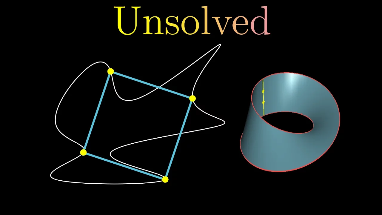
Because unordered point pairs on a loop form a Möbius strip that is topologically forced to self-intersect when anchored to a plane, every continuous closed loop is guaranteed to contain the vertices of a rectangle.

AI-assisted summary of Who cares about topology? (Old version) — original source. Check the original for full context.

Source published:

Key ideas

  • The inscribed square problem remains an open question in mathematics, asking whether every closed loop contains four points forming a square. (1:20)
  • By relaxing the condition to finding an inscribed rectangle, the question reduces to finding two distinct point pairs that share both an identical midpoint and equal separation distance. (1:20)
  • The configuration space of all unordered pairs of points on a 1D closed loop naturally forms a 2D Möbius strip, whose boundary corresponds to degenerate pairs of identical points. (11:38)
  • Mapping this Möbius strip into 3D space by midpoint and distance forces a self-intersection because its boundary lies flat in the plane, rigorously guaranteeing an inscribed rectangle. (14:39)

Detailed notes

## Background This video was published on YouTube by 3Blue1Brown (Grant Sanderson) on November 4, 2016. The description notes that this is an older version of the presentation and directs viewers to an updated release.

## TL;DR Addressing the common critique that introductory topology is reduced to playful novelties like twisting paper strips and morphing coffee mugs into donuts, Grant Sanderson illustrates the discipline's genuine problem-solving power using the inscribed rectangle problem. By weakening the unsolved inscribed square problem to rectangles, the challenge reduces to identifying two distinct pairs of points on an arbitrary closed loop that share both a midpoint and separation distance. Sanderson parameterizes all unordered pairs of points on the loop into an abstract configuration space, proving this space is topologically equivalent to a Möbius strip whose boundary corresponds to degenerate identical pairs. Mapping this strip into three-dimensional space anchors its single boundary to the flat loop, topologically compelling the surface to self-intersect and mathematically guaranteeing the existence of an inscribed rectangle.

## Atmosphere & style The presentation carries an intellectually vindicating and reflective tone, beginning with relatable skepticism toward shallow classroom parlor tricks before blooming into an elegant mathematical revelation. Sanderson's delivery is calm, clear, and deliberately paced, balancing intricate topological surgeries with lucid visual metaphors. Watching the argument unfold feels like witnessing a conceptual magic trick where seemingly esoteric shapes suddenly snap into place as indispensable machinery for a concrete geometric proof.

## Bulletin - [01:20](https://www.youtube.com/watch?v=AmgkSdhK4K8&t=80s) The inscribed square problem remains an open question in mathematics, asking whether every closed loop contains four points forming a square. - [01:20](https://www.youtube.com/watch?v=AmgkSdhK4K8&t=80s) By relaxing the condition to finding an inscribed rectangle, the question reduces to finding two distinct point pairs that share both an identical midpoint and equal separation distance. - [11:38](https://www.youtube.com/watch?v=AmgkSdhK4K8&t=698s) The configuration space of all unordered pairs of points on a 1D closed loop naturally forms a 2D Möbius strip, whose boundary corresponds to degenerate pairs of identical points. - [14:39](https://www.youtube.com/watch?v=AmgkSdhK4K8&t=879s) Mapping this Möbius strip into 3D space by midpoint and distance forces a self-intersection because its boundary lies flat in the plane, rigorously guaranteeing an inscribed rectangle.

## Key takeaways - [00:04](https://www.youtube.com/watch?v=AmgkSdhK4K8&t=4s) Traditional popular introductions to topology often focus on parlor tricks like paper Möbius strips or coffee mugs turning into donuts without demonstrating their problem-solving utility. - [01:20](https://www.youtube.com/watch?v=AmgkSdhK4K8&t=80s) The inscribed square problem asks whether any closed, continuous loop in space contains four vertices that form a square, a problem modern mathematics still cannot prove or disprove. - [01:20](https://www.youtube.com/watch?v=AmgkSdhK4K8&t=80s) Weakening the square problem to an inscribed rectangle allows mathematicians to search for two pairs of points sharing an identical midpoint and equal Euclidean distance. - [03:37](https://www.youtube.com/watch?v=AmgkSdhK4K8&t=217s) Evaluating pairs of points on a loop by plotting their midpoint on the xy-plane and their distance as vertical height sweeps out a continuous 2D surface in 3D space. - [03:37](https://www.youtube.com/watch?v=AmgkSdhK4K8&t=217s) A self-intersection or collision on this 3D surface guarantees that two distinct pairs share the same midpoint and distance, directly yielding an inscribed rectangle. - [05:51](https://www.youtube.com/watch?v=AmgkSdhK4K8&t=351s) The configuration space parameterizing ordered pairs of points on a closed loop is topologically equivalent to a torus. - [10:05](https://www.youtube.com/watch?v=AmgkSdhK4K8&t=605s) Because the distance and midpoint between two points are symmetric, ordered pairs would cause trivial collisions, necessitating a reduction to unordered pairs. - [10:05](https://www.youtube.com/watch?v=AmgkSdhK4K8&t=605s) Folding the torus coordinate square along the diagonal line y = x identifies pairs (x, y) with (y, x), leaving the diagonal crease as the degenerate pairs (x, x). - [11:38](https://www.youtube.com/watch?v=AmgkSdhK4K8&t=698s) Gluing the remaining boundary edges together requires a half-twist, proving that the space of unordered pairs on a loop is a Möbius strip. - [11:38](https://www.youtube.com/watch?v=AmgkSdhK4K8&t=698s) The single boundary edge of the Möbius strip consists entirely of degenerate pairs (x, x) where the distance between points is zero. - [13:08](https://www.youtube.com/watch?v=AmgkSdhK4K8&t=788s) When mapping the Möbius strip to 3D space using the midpoint-distance function, its boundary edge maps directly onto the original loop in the xy-plane. - [14:39](https://www.youtube.com/watch?v=AmgkSdhK4K8&t=879s) It is mathematically impossible to map a Möbius strip into 3D space with its boundary pinned to a 2D plane without the interior intersecting itself. - [14:39](https://www.youtube.com/watch?v=AmgkSdhK4K8&t=879s) The forced topological self-intersection of the Möbius strip provides the exact collision needed to prove every closed loop contains an inscribed rectangle. - [14:39](https://www.youtube.com/watch?v=AmgkSdhK4K8&t=879s) Abstract topological objects like the torus and Möbius strip are not mere mathematical curiosities, but essential configuration spaces that resolve concrete geometric problems.

## Detailed walkthrough ### [00:04](https://www.youtube.com/watch?v=AmgkSdhK4K8&t=4s) Why Topology Matters: Beyond Paper Strips and Donuts

Popular mathematical outreach often introduces topology to young students with tactile party tricks, yet these demonstrations frequently fail to convey what the discipline actually achieves. Reflecting on attending math talks and seminars as a kid, Grant Sanderson recalls how organizers consistently leaned on topology to spark enthusiasm, demonstrating objects like the Möbius strip by taking a strip of construction paper, giving it a half twist, and gluing the ends together. Students were prompted to trace a pencil along the paper to prove it had only one side, or were told the classic cliché that topologists cannot distinguish between a coffee mug and a donut because both share exactly one hole. Yet for a mathematically curious mind, these parlor tricks felt hollow. As Sanderson recalls thinking at the time, “How is this math?” and “How does any of this actually help to solve problems?”

The purpose and potency of topological reasoning remained elusive until encountering a concrete, unsolved question in geometry—the inscribed square problem—paired with an unexpectedly brilliant topological solution to its slightly relaxed counterpart. The elegant machinery used to resolve that problem reveals why mathematicians care about abstract shapes, continuous deformations, and high-dimensional surfaces. Rather than being an idle study of playdough geometry, topology provides structural invariants and spatial relationships that cut through seemingly intractable geometric questions.

[01:20](https://www.youtube.com/watch?v=AmgkSdhK4K8&t=80s) The Inscribed Square Problem and Weakening to Rectangles

The classic inscribed square problem begins with an arbitrary closed loop drawn in space—a path squiggled through space in any imaginable, convoluted manner that eventually terminates where it began. The challenge is deceptively simple to state: does every single closed loop contain four points that form the vertices of a square? For elementary geometries, the answer is trivially affirmative. A standard circle contains infinitely many inscribed squares, and an ellipse similarly accommodates inscribed squares without difficulty. The real crux of the problem lies in universality: does every possible closed loop, regardless of how jagged or pathological, possess at least one inscribed square? Describing the mystique of this open question, Sanderson remarks, “I mean, just the fact that this is unsolved is interesting, that the current tools of math can neither confirm nor deny that there's some loop with no inscribed square in it.”

```mermaid flowchart TD accTitle: Inscribed Rectangle Problem Reduction accDescr: Flowchart illustrating how finding an inscribed rectangle on a closed loop is reduced to finding collisions on a 3D surface.

subgraph LoopGeometry ["Loop & Point Pair Geometry"] A["Closed Loop in xy-Plane"] --> B["Select Two Pairs: AC and BD"] B --> C{"Do AC and BD share a midpoint<br/>AND have equal distance?"} end

subgraph GeometricCondition ["Rectangle Equivalence"] C -->|"Yes"| D["Points A, B, C, D<br/>form a Rectangle"] end

subgraph TopologicalEncoding ["3D Graph Encoding"] B --> E["Map Pair to 3D Point:<br/>(Midpoint, Distance)"] E --> F["Continuous Surface Hugs Loop"] F --> G["Self-Intersection / Collision<br/>(Two Pairs -> Same 3D Point)"] end

G -->|"Guarantees"| D ```

Because the square problem remains unproven, mathematicians look at a slightly weaker condition: finding an inscribed rectangle instead of a square. While still remarkably difficult, the rectangle version admits a breathtaking solution that Sanderson highlights as perhaps his favorite piece of mathematics. The breakthrough relies on reframing the question away from tracking four individual vertices to analyzing pairs of points. Any rectangle with vertices labeled $A$, $B$, $C$, and $D$ in cyclic order possesses two diagonals, $AC$ and $BD$. Elementary geometry dictates two fundamental properties for these diagonals: - The distance between $A$ and $C$ equals the distance between $B$ and $D$. - The midpoint of segment $AC$ coincides exactly with the midpoint of segment $BD$.

Crucially, this condition works in both directions. If two distinct pairs of points in space share an identical midpoint and have identical Euclidean lengths, the four endpoints are guaranteed to form a rectangle. Consequently, the challenge reduces to proving that every closed loop admits at least two distinct pairs of points possessing both a shared midpoint and the same separation distance.

[03:37](https://www.youtube.com/watch?v=AmgkSdhK4K8&t=217s) Mapping Point Pairs to a 3D Surface

To prove the existence of two pairs sharing both distance and midpoint, one can translate the geometry into a continuous function mapping pairs of points on the loop into single points in three-dimensional space. Picture the closed loop resting flat on the $xy$-plane. For any chosen pair of points on this loop, locate their midpoint $m$ on the $xy$-plane and measure the Euclidean distance $d$ between them. Then, plot a point in 3D space positioned at horizontal coordinate $m$ and elevated directly in the vertical $z$-direction by a height equal to $d$. Evaluating this function across all possible pairs of points sweeps out a continuous two-dimensional surface hovering above the plane.

This generated surface exhibits an intimate relationship with the underlying curve: - As two chosen points slide closer and closer together along the loop, their separation distance $d$ drops toward zero, driving the height of the plotted point down toward the plane. - Concurrently, their midpoint $m$ converges directly onto the boundary of the loop itself. - When the pair coincides into an identical point $(x, x)$, the distance is zero and the midpoint is $x$, meaning the plotted surface touches down right along the original loop.

Furthermore, this construction forms a continuous function; a minor nudge to either input point results in only a minor shift in the plotted 3D point without sudden jumps. The entire geometric existence question now hinges on whether this surface must cross itself. As Sanderson summarizes the objective, “Our goal, then, is to show that this function has a collision, that two distinct pairs of points each map to the same spot in 3D space.” If two distinct pairs produce the exact same 3D coordinate, they necessarily share the same horizontal midpoint and the same vertical height (distance), immediately yielding an inscribed rectangle.

[05:51](https://www.youtube.com/watch?v=AmgkSdhK4K8&t=351s) Constructing the Torus: The Space of Ordered Pairs

Proving that the 3D surface must intersect itself requires constructing an abstract configuration space that catalogs all possible pairs of points on the loop. In standard Cartesian geometry, pairs of real numbers are plotted on a 2D coordinate plane. By analogy, topologists look for a two-dimensional surface that naturally parameterizes every pair of points on a loop. A critical preliminary distinction must be made between ordered pairs and unordered pairs: - An **ordered pair** treats $(A, B)$ as distinct from $(B, A)$, preserving the concept of a "first" point. - An **unordered pair** treats $\{A, B\}$ as identical to $\{B, A\}$, caring solely about the selected points regardless of sequence.

While the ultimate proof requires unordered pairs, the conceptual stepping stone begins with ordered pairs. Start by cutting the closed loop at an arbitrary point and uncurling it into a straight line interval, scaled from $0$ to $1$. Every point on the original loop maps to a unique number in the interval $[0, 1]$, with the sole exception of the cut site, which corresponds simultaneously to both endpoints $0$ and $1$. By crossing this interval with a second $[0, 1]$ interval along a perpendicular axis, one forms a unit square $[0, 1] \times [0, 1]$. Every internal coordinate $(x, y)$ in this square represents an ordered pair of points on the original loop.

However, the perimeter of the square introduces ambiguity because $0$ and $1$ are physically the same point on the loop. Coordinates along the left edge $(0, y)$ represent the exact same loop pairs as coordinates along the right edge $(1, y)$. To restore a faithful one-to-one mapping, the left and right edges must be glued together in the same orientation, bending the square into a cylinder. By the same logic, the bottom edge $(x, 0)$ and top edge $(x, 1)$ represent identical second coordinates, requiring the top and bottom circular rims of the cylinder to be bent around and glued together. This two-stage gluing produces a torus—the surface of a donut. As Sanderson emphasizes, “The torus is to pair of points on the loop what the xy-plane is to pairs of points on the real number line.” Any slight movement on the torus corresponds to a smooth, slight adjustment of the point pair on the loop, establishing a continuous, bidirectional equivalence.

[10:05](https://www.youtube.com/watch?v=AmgkSdhK4K8&t=605s) Collapsing to Unordered Pairs: The Diagonal Fold

Although the torus elegantly parameterizes ordered pairs, it is too expansive for the rectangle problem. Because the midpoint and distance between $A$ and $B$ are identical to the midpoint and distance between $B$ and $A$, treating $(A, B)$ and $(B, A)$ as distinct inputs would produce a completely trivial collision on our 3D surface. As Sanderson puts it, “That's like saying you can always find a rectangle so long as you consider any pair of points to be a rectangle.”

To prevent such false positives, the parameter space must identify $(x, y)$ with $(y, x)$ as a single, unordered entity: - The coordinate $(0.2, 0.3)$ must be identified with $(0.3, 0.2)$. - The coordinate $(0.5, 0.7)$ must merge with $(0.7, 0.5)$. - In general, every coordinate $(x, y)$ must be identified with its reflection $(y, x)$.

Geometrically, identifying every point with its reflection across the line $y = x$ corresponds to folding the unit square in half along its main diagonal. This fold creates a triangle whose hypotenuse is the diagonal crease where $x = y$. This crease represents pairs of the form $(x, x)$—degenerate pairs where a point on the loop is paired with itself. In the visualization, Sanderson marks this crease as a prominent red line, noting that tracking this specific boundary will be essential for the remainder of the proof.

[11:38](https://www.youtube.com/watch?v=AmgkSdhK4K8&t=698s) Constructing the Möbius Strip from Unordered Pairs

To complete the space of unordered pairs on the loop, the remaining edges of the identification diagram must be glued together, specifically attaching the bottom edge to the right edge. Getting the orientation right is crucial here: points positioned toward the left of the bottom edge must glue to points toward the bottom of the right edge, while points toward the right of the bottom edge attach to points toward the top of the right edge. It feels counterintuitive and strange to visualize at first, warranting a pause to ponder how such a gluing can physically occur in space.

```mermaid flowchart TD accTitle: Gluing Unordered Pairs into a Möbius Strip accDescr: Steps showing how cutting and gluing the identification polygon results in a twisted Möbius strip with a boundary of degenerate pairs. subgraph CuttingAndGluing["Surgery on the Polygon"] A["Polygon representing pairs"] -->|"diagonal cut"| B["Cut pieces reoriented"] B -->|"glue original edges"| C["Rectangular strip"] C -->|"half-twist and glue cut edge"| D["Möbius Strip"] end subgraph BoundaryInterpretation["Geometric Meaning"] D --> E["Surface interior: distinct unordered pairs {x, y}"] D --> F["Red boundary edge: degenerate pairs (x, x)"] end ```

The clever trick to accomplish this is to make a diagonal cut across the shape, set it aside momentarily, glue the bottom and right edges together, and then reconnect the cut seam. Examining the arrow orientations on the resulting rectangular band reveals that reconnecting the cut ends cannot be done directly to form an ordinary cylinder. Instead, the band requires a half-twist before its ends can meet. Performing this operation in three-dimensional space produces a Möbius strip. Grant Sanderson highlights the beauty of this surprise:

> “The Möbius strip is to unordered pairs of points on the loop what the xy-plane is to pairs of real numbers.”

The red boundary edge running along the perimeter of the Möbius strip represents the degenerate pairs of the form $(x, x)$—instances where both selected points are identical.

- Unordered pairs of points on a 1D loop form a continuous two-dimensional manifold that is topologically a Möbius strip. - The single continuous boundary component (highlighted in red) consists strictly of pairs $(x, x)$ where the distance between the two points is zero. - This unexpected emergence of a Möbius strip demonstrates how abstract topological spaces naturally arise as configuration spaces of simple geometric objects.

---

[13:08](https://www.youtube.com/watch?v=AmgkSdhK4K8&t=788s) Mapping the Möbius Strip to 3D Space and the Boundary Condition

With a continuous, one-to-one correspondence established between unordered pairs of points on the loop and points across the Möbius strip, the inscribed rectangle problem can finally be addressed. The problem setup uses a special three-dimensional graph where the original loop sits flat on the $xy$-plane. For any pair of points on the loop, one finds their midpoint $m$ on the $xy$-plane and computes their Euclidean distance $d$. A point is then plotted in three-dimensional space at a height of exactly $d$ units directly above the midpoint $m$.

```mermaid flowchart LR accTitle: The Midpoint-Distance Mapping accDescr: Pipeline mapping pairs of points on a loop through the Möbius strip to a 3D surface. subgraph LoopDomain["Points on Loop"] P["Pair {x, y}"] end subgraph MobiusDomain["Möbius Strip"] M["Point on Möbius strip"] end subgraph Target3D["3D Space (z >= 0)"] S["Point (m, d):<br/>Midpoint m in xy-plane,<br/>Height d = dist(x, y)"] end P <--> M M --> S ```

Because of the continuous bijection between unordered pairs and points on the Möbius strip, this geometric construction defines a natural continuous map from the Möbius strip onto a surface in 3D space: take any point on the Möbius strip, identify the pair of points on the loop it represents, and evaluate the midpoint-and-distance function on that pair.

The boundary behavior of this mapping is the linchpin of the argument. As two points on the loop move closer together, their distance $d$ approaches zero, meaning the plotted point sinks toward the $xy$-plane directly above the loop itself. In the extreme case of pairs like $(x, x)$, the distance is zero and the midpoint is simply the point $x$ itself, placing the output directly on the loop. Consequently, when the Möbius strip is mapped into 3D space, its single boundary edge must be mapped directly onto the original closed loop sitting in the $xy$-plane.

- Input: an unordered pair $\{x, y\}$ from the loop. - Output: a point $(m_x, m_y, d)$ in $\mathbb{R}^3$, where $m = \frac{x+y}{2}$ and $d = \|x - y\|$. - Degenerate boundary pairs $(x, x)$ have $d = 0$ and $m = x$, anchoring the entire boundary of the Möbius strip seamlessly to the original loop in the plane $z = 0$.

---

[14:39](https://www.youtube.com/watch?v=AmgkSdhK4K8&t=879s) Self-Intersection and the Solution to the Inscribed Rectangle Problem

The topological crux of the proof comes down to a fundamental physical and mathematical constraint: you cannot take a Möbius strip and glue its boundary edge down onto a flat two-dimensional plane without forcing the interior of the strip to intersect itself. Because the boundary edge must match the loop in the $xy$-plane, the surface spanning that boundary must cross through itself somewhere in the space above.

> “Since points of the Möbius strip represent pairs of points on the loop, if the strip intersects itself during this mapping, it means that there are at least two distinct pairs of points that correspond to the same output on this surface, which means they share a midpoint and are the same distance apart, which in turn means that they form a rectangle.”

```mermaid flowchart TD accTitle: Topological Intersection Yields a Rectangle accDescr: Logical deduction showing how self-intersection of the Möbius strip guarantees an inscribed rectangle. A["Möbius boundary mapped to 2D loop"] --> B["Strip is topologically forced to self-intersect"] B --> C["Two distinct pairs map to identical (m, d)"] C --> D["Pairs share midpoint m and distance d"] D --> E["Four points form a rectangle on the loop"] ```

That single topological self-intersection resolves the entire inscribed rectangle problem. While the visual intuition that a Möbius strip must self-intersect when bounded by a planar curve seems clear, establishing it rigorously is precisely why the field of topology was developed. Sanderson notes that for students taking topology in the future, proving this rigorously is an illuminating exercise that clarifies why topologists construct technical definitions the way they do. He emphasizes that these shapes are far more than idle curiosities:

> “The reason for talking about the torus and the Möbius strip was not because we were playing around with construction paper, or because we were daydreaming about deforming a coffee mug.”

Rather, these surfaces emerge organically as the configuration spaces required to solve concrete, tangible geometry problems.

- A self-intersection point $(m, d)$ on the mapped surface represents two distinct unordered pairs, $\{A, B\}$ and $\{C, D\}$. - Both segments $AB$ and $CD$ have identical lengths ($d$) and bisect each other at the exact same midpoint ($m$). - Any two line segments that share a midpoint and have equal lengths define the diagonals of a rectangle, proving that the vertices $A, B, C, D$ lying on the loop form an inscribed rectangle.

## Notable quotes > [11:38](https://www.youtube.com/watch?v=AmgkSdhK4K8&t=698s) The Möbius strip is to unordered pairs of points on the loop what the xy-plane is to pairs of real numbers. — Grant Sanderson

## Mentioned Grant Sanderson, 3Blue1Brown, Möbius strip, Inscribed square problem, Inscribed rectangle problem, Torus

## Video description There’s now an updated version: https://youtu.be/IQqtsm-bBRU

[Source](https://www.youtube.com/watch?v=AmgkSdhK4K8)

中文简报

莫比乌斯带映射证明任意闭合回路必内接矩形 由于回路上的无序点对构成莫比乌斯带,且当该带锚定在平面上时在拓扑上必然发生自交,因此任意连续闭合回路必然包含矩形的顶点。 针对初等拓扑常被简化为扭转纸条、将咖啡杯形变为甜甜圈等趣味把戏的常见批评,格兰特·桑德森(Grant Sanderson)以“内接矩形问题”展示了该学科真正的解题实力。通过将尚未解决的“内接正方形问题”放宽为矩形,该难题便转化为在任意闭合回路上找出两对具有相同中点和相同距离的不同点对。桑德森将回路上所有无序点对参数化为一个抽象的构型空间,并证明该空间在拓扑上等价于莫比乌斯带,其边界对应于重合的退化点对。将这条莫比乌斯带映射到三维空间会将其唯一的边界锚定在平面的闭合回路上,从而在拓扑上迫使该曲面发生自交,在数学上严格保证了内接矩形的存在。 内接正方形问题仍是数学中未解决的开放性问题,即任意闭合回路是否都包含能构成正方形的四个点。 (1:20) 通过将条件放宽为寻找内接矩形,问题转化为寻找两对具有相同中点且距离相等的不同点对。 (1:20) 一维闭合回路上所有无序点对的构型空间自然形成一个二维莫比乌斯带,其边界对应于同一顶点的退化点对。 (11:38) 以中点和距离为参数将该莫比乌斯带映射到三维空间,由于其边界平躺在平面内,曲面被迫发生自交,从而严格保证了内接矩形的存在。 (14:39)

Reading summary

Grant Sanderson argues that topology is not merely an idle study of paper tricks and deformed coffee mugs, but a powerful mathematical framework whose abstract surfaces arise naturally to solve tangible geometric problems. Reframing Inscribed Rectangles as Point Pairs (1:20) The classic inscribed square problem asks whether every arbitrary closed loop in space contains four points that form the vertices of a square. While the square problem remains an open question that current mathematical tools can neither confirm nor deny, mathematicians study a relaxed version: proving every closed loop contains an inscribed rectangle. Sanderson explains that any rectangle $ABCD$ has diagonals $AC$ and $BD$ that share an identical midpoint and have equal Euclidean lengths, a condition that works in both directions. Consequently, the challenge reduces to proving that every closed loop admits at least two distinct pairs of points possessing both a shared midpoint and the same distance. Mapping Loop Pairs to a 3D Surface (3:37) To analyze these pairs, the geometry is translated into a continuous function mapping pairs of points on a loop lying in the $xy$-plane into three-dimensional coordinates. For any pair, its midpoint $m$ is plotted in the $xy$-plane with an elevation $z$ equal to the separation distance $d$ between the points. As the two points slide closer together, their separation drops to zero and the midpoint converges onto the loop boundary. When evaluated across all possible pairs, this continuous function sweeps out a surface in 3D space. The geometric existence question hinges on whether this function produces a collision: if two distinct pairs map to the exact same 3D coordinate, they share a midpoint and distance, immediately forming an inscribed rectangle. The Möbius Strip as an Unordered Configuration Space (10:05) Finding collisions requires constructing an abstract configuration space of all point pairs. Cutting the loop and parameterizing it as a unit square $[0, 1] \times [0, 1]$ initially forms a torus when opposite edges are glued, representing ordered pairs $(x, y)$. However, because midpoint and distance are symmetric, treating $(A, B)$ and $(B, A)$ as distinct inputs produces trivial collisions. Identifying each coordinate with its reflection $(y, x)$ corresponds to folding the square across its main diagonal, where the crease represents degenerate pairs $(x, x)$. Gluing the remaining edges together requires a half-twist, yielding a Möbius strip whose single continuous boundary represents these degenerate pairs where separation distance is zero. Topological Self-Intersection Solves the Problem (14:39) Mapping this Möbius strip into 3D space assigns every point to its corresponding midpoint and distance coordinates. Because degenerate pairs along the boundary have zero distance, the entire boundary of the Möbius strip is anchored directly to the original closed loop resting flat on the $xy$-plane. Mathematically, a Möbius strip cannot have its boundary glued flat onto a two-dimensional plane without forcing its interior to intersect itself. This unavoidable self-intersection means that at least two distinct unordered pairs of points map to the exact same 3D coordinate $(m, d)$, proving they share a midpoint and length and thereby guaranteeing an inscribed rectangle. While the relaxed rectangle problem is fully resolved through topological intersection, the original inscribed square problem remains unsolved. Sanderson notes that rigorous proofs of these self-intersections illustrate why formal topology was developed, showing that surfaces like the torus and Möbius strip function as vital configuration spaces rather than frivolous novelties.

精炼阅读摘要

Grant Sanderson指出,拓扑学常被科普简化为折纸条或将咖啡杯变形为甜甜圈的演示,但其本质是解决棘手几何难题的结构工具。通过将未解的“内接正方形问题”弱化为“内接矩形问题”,数学家利用拓扑配置空间与连续映射,证明了任意闭合回路都必然存在内接矩形。 内接正方形问题的弱化与对角线等价性 (1:20) 经典内接正方形问题探讨空间中任意一条闭合回路是否都包含四个能构成正方形顶点的点。圆和椭圆等规则几何图形显然满足该条件,但Sanderson指出,目前的数学工具既无法证实也无法证伪是否存在没有任何内接正方形的病态闭合曲线,该猜想至今仍未解决。为寻求突破,数学家转向解决其稍弱的形式——寻找内接矩形。 解决内接矩形问题的关键在于将追踪四个顶点的任务转化为分析两对点。若四边形四个顶点按顺序为A、B、C、D,则线段AC与BD构成其对角线。根据初等几何性质,四边形为矩形当且仅当其两条对角线长度相等且中点完全重合。这意味着寻找内接矩形等价于在曲线上寻找两对截然不同的点,使它们具备完全相同的中点与欧式距离。 三维中点高度映射与碰撞条件 (3:37) 为了在任意闭合曲线上找到符合条件的两对点,可将几何条件转化为三维空间中的连续函数。假设闭合回路平铺在xy平面上,针对曲线上任意选定的一对点,在xy平面标出它们的中点m,并测量两点间的欧式距离d。随后在三维空间中绘制一个点:其水平位置为m,垂直方向的高度z则等于距离d。遍历曲线上所有的点对,即可在平面上方生成一张连续的二维曲面。 当两个点在回路上逐渐靠近时,它们的间距d趋向于零,高度随之降向底面;当两点最终重合成同一点(x, x)时,间距为零且中点即为x本身,该曲面的边界因而直接贴合在xy平面的闭合回路上。若该三维曲面发生自相交(即产生“碰撞”),便意味着曲线上存在两个不同的点对映射到了同一个三维坐标(m, d),从而证明它们拥有相同的中点和相等的间距,必然构成内接矩形。 点对配置空间:从环面到莫比乌斯环 (5:51) 分析该曲面是否必然自交,需要为回路上的点对构建抽象的配置空间。若先分析有序点对,可将闭合回路剪开拉直为[0, 1]区间,两端点代表回路上的同一个剪切点。两个[0, 1]区间做笛卡尔积可形成单位正方形,内部每个坐标均对应一个有序点对。将正方形左右边缘同向粘合可得到圆柱体,再将上下圆环边缘同向粘合,便形成了一个环面。环面之于回路上的点对,正如xy平面之于实数对。 然而,有序点对会将(A, B)和(B, A)视为不同输入,但二者具有完全相同的中点和距离,这会导致无意义的虚假碰撞。为了排除假象,必须采用无序点对,将坐标(x, y)与其对称点(y, x)重合,这相当于把正方形沿对角线折叠成三角形。由于原正方形的边界仍需粘合,经过对折与方向适配,带子在连接前必须经过一次半扭转,其结果在拓扑结构上正是一个莫比乌斯环。莫比乌斯环唯一的连续边界正好对应所有距离为零的重合点对(x, x)。 拓扑自相交与内接矩形的存在性证明 (14:39) 将莫比乌斯环作为配置空间映射到三维空间时,该几何问题触碰到了深刻的拓扑学硬约束。根据前述高度映射关系,莫比乌斯环的唯一外围边界完全落在了xy平面的闭合回路上。拓扑学定理表明:在三维空间中,无法在不发生内部自相交的情况下,将莫比乌斯环的边界完全粘在一个二维平面闭合回路上。 由于边界被强制锚定在平面回路上,悬浮在平面上方的莫比乌斯环曲面必然会在某处穿过自身。曲面自交点意味着至少存在两个不同的无序点对{A, B}与{C, D}映射到了同一个三维点(m, d)。因此,线段AB与CD不仅长度相同,而且拥有共同的中点,这四点必然构成回路上的一个内接矩形。 Sanderson总结道,莫比乌斯环与环面并非手工纸条游戏或无意义的几何遐想,而是作为解决具体空间问题的配置空间自然涌现。尽管普遍的内接正方形问题在当前数学体系中仍悬而未决,但内接矩形问题的拓扑学证明展示了高维流形与连续形变工具如何能够穿透看似无从下手的经典几何难题。

Detailed notes — zh

## Background 本内容由著名数学科普频道 3Blue1Brown 于 2016 年 11 月 4 日发布在 YouTube 平台上。视频简介指出这是该主题的旧版视频,并附上了后续重新制作的更新版本链接。 ## TL;DR 视频从许多人在初次接触拓扑学时常有的困惑(“这到底算什么数学?它能解决什么实际问题?”)切入,聚焦于著名的未解之谜“内接正方形猜想”。随后,主讲人探讨了其弱化版本——内接矩形问题,并展示了一个极为精妙的拓扑学证明。通过将闭合回路上的有序点对映射为环面、无序点对映射为莫比乌斯带,主讲人证明了该曲面在特定三维映射下必然发生自相交,从而确凿证明了任意闭合回路上都必然存在内接矩形。最终,视频阐明了莫比乌斯带与环面并非脱离实际的几何玩具,而是解决具体难题时自然涌现的强大数学工具。 ## Atmosphere & style 整部视频洋溢着 3Blue1Brown 标志性的沉稳、优雅与极具启发性的叙事风格。主讲人 Grant Sanderson 的语调温和而充满感染力,引导观众从童年做手工折纸纸带的困惑出发,逐步抽丝剥茧,跨入高维抽象空间的壮丽景观。观看体验宛如经历一场层层递进的思维顿悟(Aha! moment)——当原本零散的几何点对最终不可思议地扭转缝合成一条莫比乌斯带并击破证明难题时,带给观众的是极致纯粹的数学美感与智力震撼。 ## Bulletin - [00:04](https://www.youtube.com/watch?v=AmgkSdhK4K8&t=4s) 内接正方形问题(在任意闭合回路上寻找四个能构成正方形的点)至今仍是未解之谜,但其弱化版本——内接矩形问题,可以通过拓扑学得到完美证明。 - [02:13](https://www.youtube.com/watch?v=AmgkSdhK4K8&t=133s) 证明内接矩形的关键在于将几何问题转化为拓扑自交问题:通过将回路上的点对映射到三维空间,寻找共享相同中点和距离的两个不同点对。 - [11:38](https://www.youtube.com/watch?v=AmgkSdhK4K8&t=698s) 闭合回路上的无序点对在拓扑上等价于莫比乌斯带,其边界对应于重合的点对 (x, x)。 - [13:08](https://www.youtube.com/watch?v=AmgkSdhK4K8&t=788s) 莫比乌斯带的特殊单侧扭转结构决定了其边界在贴合到二维平面时必然发生自相交,从而在几何上证明了任意闭合回路上必然存在内接矩形。 ## Key takeaways - [00:04](https://www.youtube.com/watch?v=AmgkSdhK4K8&t=4s) 许多人对拓扑学的初次印象停留在莫比乌斯带或“咖啡杯等同于甜甜圈”的趣味展示,这常让人困惑拓扑学在实际数学中如何解决具体问题。 - [00:04](https://www.youtube.com/watch?v=AmgkSdhK4K8&t=4s) 内接正方形问题探讨是否在任意闭合回路上都能找到四个点构成正方形,现有数学工具既不能证实也不能证伪这一命题。 - [02:13](https://www.youtube.com/watch?v=AmgkSdhK4K8&t=133s) 弱化版的“内接矩形问题”可以通过将关注点从单个点转向“点对”来寻找突破口。 - [02:13](https://www.youtube.com/watch?v=AmgkSdhK4K8&t=133s) 矩形的几何特征可转化为:两组对角顶点对必须共享同一个中点,且两点间的距离完全相等。 - [02:13](https://www.youtube.com/watch?v=AmgkSdhK4K8&t=133s) 通过定义一个三维映射函数(以两点中点为 xy 坐标,距离为 z 轴高度),内接矩形的存在性等价于证明该三维曲面存在自相交。 - [05:51](https://www.youtube.com/watch?v=AmgkSdhK4K8&t=351s) 回路上的有序点对可以通过将回路展开为 [0, 1] 区间,并构建一个单位正方形来参数化表示。 - [05:51](https://www.youtube.com/watch?v=AmgkSdhK4K8&t=351s) 将单位正方形的对边进行同向粘合,在拓扑上会自然形成一个环面(Torus),代表所有有序点对的空间。 - [10:05](https://www.youtube.com/watch?v=AmgkSdhK4K8&t=605s) 为了避免 (A, B) 和 (B, A) 被视为不同点对而产生平凡解,必须将空间过渡到无序点对。 - [10:05](https://www.youtube.com/watch?v=AmgkSdhK4K8&t=605s) 无序点对要求将正方形沿着主对角线 x=y 进行折叠,该对角线代表退化的点对 (x, x)。 - [11:38](https://www.youtube.com/watch?v=AmgkSdhK4K8&t=698s) 将折叠后的图形进行特定的定向黏合,在拓扑上会形成一个莫比乌斯带,其单侧红边对应所有重合的点对。 - [11:38](https://www.youtube.com/watch?v=AmgkSdhK4K8&t=698s) 莫比乌斯带之于回路上的无序点对,正如 xy 坐标平面之于实数对,是其天然的拓扑表示。 - [13:08](https://www.youtube.com/watch?v=AmgkSdhK4K8&t=788s) 当两点无限接近时,映射高度 d 趋于 0,这意味着莫比乌斯带的边界必须严丝合缝地映射到 xy 平面上的原始回路上。 - [13:08](https://www.youtube.com/watch?v=AmgkSdhK4K8&t=788s) 莫比乌斯带的单侧扭转结构决定了,在不发生自相交的情况下,无法将其边界黏合到二维平面上。 - [13:08](https://www.youtube.com/watch?v=AmgkSdhK4K8&t=788s) 这种被迫的自相交证明了存在两对不同的点,它们拥有相同的中点和距离,从而宣告内接矩形必然存在。 - [15:21](https://www.youtube.com/watch?v=AmgkSdhK4K8&t=921s) 拓扑学的真正价值在于它提供了一种自然理解点对空间等抽象几何结构的工具,用以解决具体的现实数学难题。 ## Detailed walkthrough ### [00:04](https://www.youtube.com/watch?v=AmgkSdhK4K8&t=4s) 拓扑学的真正意义与内接正方形猜想 作为一名热爱数学长大的学生,3Blue1Brown 的主讲人回顾了自己童年参加各种旨在激发青少年数学兴趣的讲座经历。在那些活动中,拓扑学几乎总是演讲者用来吸引大家想象力的首选题材:讲师们会拿出手工彩纸,将一条纸带扭转半圈后将两端粘贴起来,制作成莫比乌斯带(Möbius strip),并让孩子们在上面画线以证明这是一张“只有一面的曲面”;或者宣称在拓扑学家眼中,咖啡杯和甜甜圈本质上是一模一样的,因为它们都只有一个洞。然而,这类经典的展示往往会给听众留下一连串挥之不去的困惑:“How is this math? How does any of this actually help to solve problems?” 直到后来遇到了一个极其精妙且令人惊叹的数学问题及其解答,他才真正理解为什么数学家会如此在乎这些奇形怪状的几何形体及其拓扑性质。 这个问题源自著名的未解之谜——内接正方形问题(Inscribed square problem)。假设你在空间中任意绘制一条闭合回路(closed loop)——无论这条线条蜿蜒曲折得多离谱,只要它最终回到起点——核心问题是:我们是否总能在该闭合回路上找到四个点,恰好构成一个正方形?如果回路是一个完美的正圆,找到内接正方形易如反掌,实际上存在无穷多个;如果回路是椭圆,找出内接正方形也相对容易。然而,这一命题是否对任意闭合回路(无论其形状多么复杂疯狂)都普遍成立,至今仍是一个未解之谜。主讲人由衷感叹道:“I mean, just the fact that this is unsolved is interesting, that the current tools of math can neither confirm nor deny that there's some loop with no inscribed square in it.” 现有数学工具既不能证实也不能证伪是否存在某种完全无法画出内接正方形的回路。 ```mermaid flowchart TD accTitle: 矩形判定条件与回路映射逻辑 accDescr: 展示如何将矩形性质转化为点对的中点与距离匹配,并映射至三维曲面 subgraph Geometry["几何性质转化"] A["矩形 ABCD"] --> B["对角线 AC 与 BD"] B --> C["共享同一中点 m"] B --> D["两对点距离相等 d"] end subgraph Mapping["构造三维映射"] E["回路上的点对 (p1, p2)"] --> F["xy 平面上标出中点 m"] F --> G["在 z 轴抬高 d 单位: (m_x, m_y, d)"] end subgraph Goal["拓扑目标"] G --> H["连续生成三维曲面"] C & D --> I["曲面自相交 = 存在内接矩形"] H --> I end ``` ### [02:13](https://www.youtube.com/watch?v=AmgkSdhK4K8&t=133s) 弱化问题:内接矩形与三维曲面映射 面对极度棘手的正方形问题,数学家退而求其次,提出了一个稍弱的版本:任意闭合回路上是否总能找到四个点构成“内接矩形”?虽然条件放宽了,但这依然是一个极其困难的命题。然而,它却拥有一个绝妙的拓扑学证明,被主讲人誉为自己最喜欢的数学成果之一。解决该问题的关键在于思维的跃迁:不再孤立地盯住回路上的单个点,而是将目光转向“点对”(pairs of points)。 对于任意矩形 $ABCD$,对角顶点对 $AC$ 与对角顶点对 $BD$ 具备两项极其严格的共同特征:$A$ 到 $C$ 的距离等于 $B$ 到 $D$ 的距离,且 $AC$ 的中点与 $BD$ 的中点完全重合。更关键的是,这一几何特征充分必要——只要空间中存在两对独立的点 $AC$ 与 $BD$,满足“共享中点且间距相等”,这四个点就必然能构成一个矩形。因此,证明内接矩形的存在性,等价于证明:在任意闭合回路上,一定能找到两对互不相同的点,它们不仅共享同一个中点,而且两点间的距离完全相同。 为了捕获这一几何特征,主讲人构造了一个精妙的函数:将闭合回路平铺在三维空间的 $xy$ 平面上,对于回路上的任意一对点,设它们在 $xy$ 平面上的几何中点为 $m$,两点之间的空间距离为 $d$。接着,从平面中点 $m$ 垂直沿着 $z$ 轴正方向向上抬高 $d$ 个单位,绘制出点 $(m_x, m_y, d)$。当对回路上的所有点对都执行该操作时,这些点在三维空间中便织出了一张悬挂在平面的连续曲面: - 当两点相互逼近时,它们的欧几里得距离 $d$ 缩减为 0,导致曲面上的点高度持续降低;同时,它们的中点 $m$ 也无限贴近回路本身。 - 当两点完全重合(即输入为 $(x, x)$ 形式)时,距离 $d=0$,映射点精准地落在回路上的点 $x$ 处,使得整张三维曲面如同裙边一样严丝合缝地“紧抱”(hug)着底部的闭合回路。 - 该函数具备连续性(continuous):输入端点对的微小扰动只会带来三维输出点的微小位移,绝不会发生突变断裂。 - 寻找内接矩形的目标因此彻底转化为拓扑自交问题:“Our goal, then, is to show that this function has a collision, that two distinct pairs of points each map to the same spot in 3D space.” 只要能证明这张曲面必定会发生自相交(self-intersection),就意味着存在两个不同的点对具有相同的中点与距离,从而证明内接矩形必然存在。 ### [05:51](https://www.youtube.com/watch?v=AmgkSdhK4K8&t=351s) 参数化点对:从单位正方形到环面(Torus) 为了证明这张由回路点对生成的曲面必然自交,必须深入理解“回路上的所有点对”构成的拓扑空间。就像实数对 $(x, y)$ 能自然对应于二维平面直角坐标系一样,数学家需要寻找一个天然表示回路上所有点对的二维几何曲面。讨论点对时必须辨清两个概念:“有序点对”(ordered pairs,即把对 $(A, B)$ 与 $(B, A)$ 视作不同实体)和“无序点对”(unordered pairs,$(A, B)$ 与 $(B, A)$ 被视为完全相同的对象)。最终目标是要刻画无序点对,但通往终点的必经之路是首先建立有序点对的模型。 第一步是将弯曲的闭合回路剪开并拉直,变成一条线段区间,标定为实数轴上的 $[0, 1]$。这样,回路上的每个点都与区间内的唯一实数对应;唯一的例外是当初下剪刀的那个切割点,它在展开后同时对应区间的两个端点 $0$ 和 $1$。借助这一区间,可以引入第二条区间作为纵轴,二者张成一个边长为 $1 \times 1$ 的单位正方形。正方形内的每个坐标点 $(x, y)$(其中 $x, y \in [0, 1]$)都唯一对应着闭合回路上的一对有序点。 ```mermaid flowchart LR accTitle: 单位正方形粘合为环面的拓扑变换流程 accDescr: 说明通过粘合单位正方形的对边构造环面的过程 subgraph Square["单位正方形 [0, 1] x [0, 1]"] S1["左边缘 (x=0) 与 右边缘 (x=1)"] S2["底边缘 (y=0) 与 顶边缘 (y=1)"] end subgraph Step1["第一次粘合"] S1 -->|"左右边缘沿同向粘合"| CYL["圆柱面 (Cylinder)"] end subgraph Step2["第二次粘合"] CYL -->|"上下管口端对端粘合"| TOR["环面 (Torus / 甜甜圈表面)"] end ``` 然而,单位正方形的边缘存在严重的对应冗余。因为区间端点 $0$ 与 $1$ 在几何回路上本就是同一点,所以正方形左侧边缘上的点(例如 $(0, 0.1), (0, 0.2)$ 等)与右侧边缘上高度一致的点($(1, 0.1), (1, 0.2)$ 等)代表着回路上完全相同的点对。为了消除这种人为割裂,正方形的左边缘必须与右边缘粘合在一起,卷成一个圆柱面(cylinder)。同理,底部的 $y=0$ 与顶部的 $y=1$ 也对应着回路中的同一个第二点,因此圆柱体两端的圆环开口也必须弯曲对齐粘合。经过这两次同向粘合,正方形化为了一个拓扑环面(torus,即甜甜圈的表面): - 环面上的每一个点与回路上的有序点对一一双向连续对应:在环面上轻微滑动一点,回路上的一对点也会随之微调,反之亦然。 - 环面之于回路上的点对,正如 $xy$ 坐标平面之于实数对。 ### [10:05](https://www.youtube.com/watch?v=AmgkSdhK4K8&t=605s) 无序点对的要求与对角折叠 确立了环面代表有序点对后,主讲人提出了更进一步的严峻考验:既然环面只代表有序点对,那么无序点对对应的天然拓扑形状又是什么?主讲人强调,必须排除平凡解的干扰:“After all, the whole reason we're doing this is to show that two distinct pairs of pairs of points on the loop share a midpoint and are the same distance apart. But if we consider a pair AB to be distinct from BA, then that would trivially give us two separate pairs which have the same midpoint and distance apart.” 换句话说,如果把 $(A, B)$ 和 $(B, A)$ 当作两对独立的点,那么任何两点由于它们自身与自身中点重合、距离相等,就会被直接判定为一个退化的“矩形”,这在几何上毫无意义。 因此,数学模型必须严谨地过渡到无序点对: - 坐标 $(0.2, 0.3)$ 与 $(0.3, 0.2)$ 必须被视为同一个点; - 坐标 $(0.5, 0.7)$ 与 $(0.7, 0.5)$ 也必须合二为一; - 普遍而言,平面上任何坐标 $(x, y)$ 都必须与镜像对称的 $(y, x)$ 发生粘合。 在拓扑操作上,这意味着必须将单位正方形沿着主对角线进行对折。这一对折产生的折痕——即 $x = y$ 的红色对角线——所承载的全部点对都形如 $(x, x)$。它们代表的是回路上的同一点自身与自身配对(退化点对)。主讲人特别叮嘱观众牢牢记住这条被标记为红色的对角线,因为它是解开整个内接矩形存在性证明最终谜底的核心线索。 ### [11:38](https://www.youtube.com/watch?v=AmgkSdhK4K8&t=698s) 莫比乌斯带的诞生:无序点对的拓扑结构 在处理环线上所有形如 $(x, x)$ 的重合点对时,明确它们在几何图形中的位置变得尤为重要。此时,图形上仍有一些带箭头的边需要拼接。具体来说,底边需要与右侧边黏合在一起,而黏合的方向(定向)至关重要:底边偏左的点必须黏合到右侧边靠下的点,底边偏右的点则必须黏合到右侧边靠上的点。这种特殊的对齐方式十分违反直觉,正如 Grant Sanderson 所说:“It's weird to think about, right? Go ahead, pause and ponder this for a moment.” 为了清晰地完成这一操作,这里使用了一个非常巧妙的方法:先沿着对角线做一次剪切,把图形剪开,并牢记稍后必须再黏回去。切开之后,底边和右侧边就可以顺畅地贴合在一起。然而,观察切口边缘的箭头方向会发现,要将刚才切开的部分重新黏合,不能仅仅像做圆柱体那样直接把矩形两端对齐拼合,而是必须在三维空间中将其翻转扭曲一次。经过这一扭曲后所得到的几何体,正是著名的莫比乌斯带(Möbius strip)。Grant 感叹道:“The Möbius strip is to unordered pairs of points on the loop what the xy-plane is to pairs of real numbers. That totally blew my mind when I first saw it.” ```mermaid flowchart TD accTitle: 构造莫比乌斯带的过程 accDescr: 展示将正方形沿对角线剪切、翻折并最终形成莫比乌斯带的拓扑变换过程 subgraph S1["剪切与预拼接"] A["正方形区域(含 xx 边界)"] -->|"沿对角线剪切"| B["分离的多边形碎片"] B -->|"底边与右侧边定向黏合"| C["展开的带状区域"] end subgraph S2["扭转与闭合"] C -->|"定向相反的剪切边对齐"| D["三维空间中扭转 180 度"] D -->|"闭合边缘"| E["莫比乌斯带 (Möbius Strip)"] end ``` - 莫比乌斯带的表面连续且一一对应地代表了环线上所有无序点对构成的抽象空间。 - 莫比乌斯带唯一的单侧红边,恰好对应了所有 $(x, x)$ 这类实际上是同一个点被列出两次的重合点对。 ### [13:08](https://www.youtube.com/watch?v=AmgkSdhK4K8&t=788s) 映射到三维空间与自相交证明 建立了环线上无序点对与莫比乌斯带上各点之间的连续一一对应后,内接矩形问题(Inscribed Rectangle Problem)便迎刃而解。回顾此前在三维空间中定义的特殊曲面映射:环线平躺在 $xy$ 平面上,对于环线上的任意一对无序点,先找到它们在 $xy$ 平面上的中点 $m$,以及两点间的欧几里得距离 $d$,然后在高度恰好为距离 $d$ 的位置(即中点正上方 $d$ 处)画一个点。借助连续一一对应关系,便在三维空间中形成了一个从莫比乌斯带到该曲面的天然连续映射——对莫比乌斯带上的每个点,找到其代表的环线点对,再输入到这个映射函数中。 这里的核心突破口在于边界的表现:当环线上的两个点极度接近时,函数输出的高度几乎为零,位于环线正上方;而在极限情况 $(x, x)$ 下,由于距离为零,输出点完全落在 $xy$ 平面的环线本身。这意味着莫比乌斯带的红色边界必须严丝合缝地映射到 $xy$ 平面中的原始环线上。然而,从拓扑学的几何性质来看,莫比乌斯带拥有极为特殊的单侧扭转结构,“there is no way to glue its edge to something two-dimensional without forcing the strip to intersect itself.” ```mermaid flowchart LR accTitle: 拓扑映射与矩形存在性证明逻辑 accDescr: 莫比乌斯带边界贴平导致曲面自交,从而推导出两对点共享中点与距离,证明矩形存在 A["莫比乌斯带边界"] -->|"映射到二维平面"| B["边界紧贴平面环线"] B -->|"拓扑性质限制"| C["曲面被迫发生自交"] C -->|"同一点有两个来源"| D["两组不同点对具有相同 (m, d)"] D -->|"中点相同且距离相等"| E["四点构成内接矩形"] ``` - **自交的几何含义**:莫比乌斯带在三维空间映射中发生自相交,意味着曲面上至少有一个点由莫比乌斯带上至少两个完全不同的点重叠而成。 - **矩形的成立**:这意味着环线上存在两对不同的点,它们拥有完全相同的中点 $m$ 以及完全相同的两点间距离 $d$。连接同一中点且等长的两根对角线,其四个端点必然构成一个矩形,从而完整证明了任何平滑闭合环线上都必然存在内接矩形。 ### [15:21](https://www.youtube.com/watch?v=AmgkSdhK4K8&t=921s) 拓扑学的真正意义 严格论证“莫比乌斯带的边界在黏合到二维平面时必须发生自相交”看似符合直觉,但要给出无懈可击的数学证明,就必须系统化地建立并运用拓扑学。Grant 指出,对于未来打算学习拓扑学课程的学生来说,尝试严谨证明这个自交命题是一次极佳的思维训练,能让人深刻理解拓扑学家为何要建立那些抽象晦涩的定义。 在结语中,Grant 阐明了本期视频的核心主旨:数学家研究环面和莫比乌斯带,绝不是闲来无事摆弄手工折纸,也不是整天幻想把咖啡杯捏成甜甜圈。正如他总结道:“The reason for talking about the torus and the Möbius strip was not because we were playing around with construction paper, or because we were daydreaming about deforming a coffee mug. They came up as a natural way to understand pairs of points on a loop, and that's something that we needed to solve a concrete problem.” 拓扑学是在试图理清点对空间的内在几何结构时自然涌现的工具,是解决现实、具体几何难题不可或缺的强大武器。 ## Video description There’s now an updated version: https://youtu.be/IQqtsm-bBRU [Source](https://www.youtube.com/watch?v=AmgkSdhK4K8)

Source quotes

[11:38] Grant Sanderson: The Möbius strip is to unordered pairs of points on the loop what the xy-plane is to pairs of real numbers.

Original transcript

[0:04] I've got several fun things for you this video. [0:07] An unsolved problem, a very elegant solution to a weaker version of the problem, [0:11] and a little bit about what topology is and why people care. [0:15] But before I jump into it, it's worth saying a [0:17] few words on why I'm excited to share this solution. [0:20] When I was a kid, since I loved math and sought out various mathy things, [0:24] I would occasionally find myself in some talk or a seminar where people [0:28] wanted to get the youth excited about things that mathematicians care about. [0:33] A very common go-to topic to excite our imaginations was topology. [0:38] We might be shown something like a mobius strip, [0:40] maybe building it out of construction paper by twisting a rectangle and gluing its ends. [0:45] Look, we'd be told, as we were asked to draw a line along the surface. [0:49] It's a surface with just one side. [0:52] Or we might be told that topologists view coffee mugs and donuts as the same thing, [0:57] since each has just one hole. [0:59] But these kinds of demos always left a lurking question. [1:03] How is this math? [1:04] How does any of this actually help to solve problems? [1:07] It wasn't until I saw the problem that I'm about to show you, [1:10] with its elegant and surprising solution, that I started to understand why [1:14] mathematicians actually care about some of these shapes and the properties they have. [1:20] So, there's this unsolved problem called the inscribed square problem. [1:25] If you have a closed loop, meaning you squiggle some line through space in a [1:28] potentially crazy way and you end up back where you started, [1:32] the question is whether or not you'll always be able to find four points on this [1:36] loop that make up a square. [1:38] If your closed loop was a circle, for example, [1:40] it's quite easy to find an inscribed square. [1:43] Infinitely many, in fact. [1:48] If your loop was instead an ellipse, it's still pretty easy to find an inscribed square. [1:54] The question is whether or not every possible closed loop, [1:57] no matter how crazy, has at least one inscribed square. [2:01] Pretty interesting, right? [2:03] I mean, just the fact that this is unsolved is interesting, [2:06] that the current tools of math can neither confirm nor deny that there's some loop with [2:11] no inscribed square in it. [2:13] Now, if we weaken the question a bit and ask about inscribed rectangles [2:18] instead of inscribed squares, it's still pretty hard, but there is a beautiful, [2:22] video-worthy solution that might actually be my favorite piece of math. [2:28] The idea is to shift the focus away from individual [2:31] points on the loop and instead onto pairs of points. [2:34] We'll use the following fact about rectangles. [2:37] Let's label the vertices of some rectangle ABCD. [2:41] Then the pair of points AC has a few things in common with the pair of points BD. [2:47] The distance between A and C equals the distance between B and D, [2:51] and the midpoint of A and C is the same as the midpoint of B and D. [2:56] In fact, any time you have two separate pairs of points in space, AC and BD, [3:01] if you can guarantee that they share a midpoint and that the distance between AC equals [3:06] the distance between B and D, it's enough to guarantee that those four points make up [3:12] a rectangle. [3:14] So what we're going to do is try to prove that for any closed loop, [3:18] it's always possible to find two distinct pairs of points on that [3:21] loop that share a midpoint and which are the same distance apart. [3:25] Take a moment to make sure that's clear. [3:27] We're finding two distinct pairs of points that share [3:30] a common midpoint and which are the same distance apart. [3:37] The way we'll go about this is to define a function that takes [3:41] in pairs of points on the loop and outputs a single point in 3D space, [3:45] which kind of encodes the midpoint and distance information. [3:49] It will be sort of like a graph. [3:52] Consider the closed loop to be sitting on the xy-plane in 3D space. [3:57] For a given pair of points, label their midpoint m, [4:00] which will be some point on the xy-plane, and label the distance between them d. [4:06] Plot the point, which is exactly d units above that midpoint m in the z-direction. [4:14] As you do this for many possible pairs of points, [4:17] you'll effectively be drawing through 3D space. [4:21] And if you do it for all possible pairs of points on the loop, [4:24] you'll draw out some kind of surface above the plane. [4:28] Now look at the surface, and notice how it seems to hug the loop itself. [4:33] This is actually going to be important later, so let's think about why it happens. [4:38] As the pair of points on the loop gets closer and closer, the plotted point gets lower, [4:43] since its height is by definition equal to the distance between the points. [4:47] Also, the midpoint gets closer and closer to the loop as the points approach each other. [4:53] Once the pair of points coincides, meaning the input of our [4:56] function looks like xx for some point x on the loop, [4:59] the plotted point of the surface will be exactly on the loop at the point x. [5:05] Okay, so remember that. [5:07] Another important fact is that this function is continuous, [5:10] and all that really means is that if you slightly adjust a given pair of points, [5:14] then the corresponding output in 3D is only slightly adjusted as well. [5:19] There's never a sudden discontinuous jump. [5:22] Our goal, then, is to show that this function has a collision, [5:26] that two distinct pairs of points each map to the same spot in 3D space. [5:31] Because the only way for that to happen is if they share a common midpoint, [5:35] and if their distance d apart from each other is the same. [5:40] So in some sense, finding an inscribed rectangle comes [5:43] down to showing that this surface has to intersect itself. [5:51] To move forward from here, we need to build up a [5:54] relationship with the idea of pairs of points on a loop. [5:58] Think about how we represent pairs of real numbers [6:01] using a two-dimensional coordinate plane. [6:08] Analogous to this, we're going to seek out a certain 2D surface [6:11] which naturally represents all pairs of points on the loop. [6:15] Understanding the properties of this surface will help to show [6:18] why the graph that we just defined has to intersect itself. [6:23] Now, when I say pair of points, there are two things that I could be talking about. [6:27] The first is ordered pairs of points, which would mean a [6:30] pair like AB would be considered distinct from the pair BA. [6:34] That is, there's some notion of which point is the first one. [6:39] The second idea is unordered points, where AB and BA would be considered the same thing, [6:44] where all that really matters is what the points are, [6:47] and there's no meaning to which one is first. [6:51] Ultimately, we want to understand unordered pairs of points, [6:53] but to get there, we need to take a path of thought through ordered pairs. [6:59] We'll start out by straightening out the loop, [7:01] cutting it at some point, and deforming it into an interval. [7:05] For the sake of having some labels, let's say that [7:07] this is the interval on the number line from 0 to 1. [7:11] By following where each point ends up, every point on the loop corresponds with a [7:16] unique number on this interval, except for the point where the cut happened, [7:21] which corresponds simultaneously to both endpoints of the interval, [7:25] meaning the numbers 0 and 1. [7:28] Now, the benefit of straightening out this loop like this is that we can start [7:32] thinking about pairs of points the same way we think about pairs of numbers. [7:38] Make a y-axis using a second interval, then associate each pair of values [7:43] on the interval with a single point in this 1x1 square that they span out. [7:49] Every individual point of this square naturally corresponds to a pair of [7:54] points on the loop, since its x and y coordinates are each numbers between 0 and 1, [7:58] which are in turn associated to some unique point on the loop. [8:03] Remember, we're trying to find a surface that naturally represents the set of [8:07] all pairs of points on the loop, and this square is the first step to doing that. [8:12] The problem is that there's some ambiguity when it comes to the edges of the square. [8:17] Remember, the endpoints 0 and 1 on the interval really correspond to [8:21] the same point of the loop, as if to say that those endpoints need to [8:25] be glued together if we're going to faithfully map back to the loop. [8:29] So all of the points on the left edge of the square, like 0, 0, 0.1, 0, 0.2, [8:35] on and on and on, really represent the same pair of points on the loop as the [8:40] corresponding coordinates on the right edge of the square, 1, 0.1, 1, 0.2, [8:45] on and on and on. [8:47] So for this square to represent the pairs of points on the loop in a unique way, [8:51] we need to glue this left edge to the right edge. [8:55] I'll mark each edge with some arrows to remember how the edges need to be lined up. [9:00] Likewise, the bottom edge needs to be glued to the top edge, [9:04] since y-coordinates of 0 and 1 really represent the same second point in a given pair [9:08] of points on the loop. [9:13] If you bend this square to perform the gluing, [9:16] first rolling it into a cylinder to glue the left and right edges, [9:20] then gluing the ends of that cylinder, which represent the top and bottom edges, [9:24] we get a torus, better known as the surface of a doughnut. [9:29] Every individual point on this torus corresponds to a unique pair of points on the loop, [9:34] and likewise, every pair of points on the loop corresponds to [9:38] some unique point on this torus. [9:40] The torus is to pair of points on the loop what the [9:43] xy-plane is to pairs of points on the real number line. [9:49] The key property of this association is that it's continuous both ways, [9:53] meaning if you nudge any point on the torus by just a tiny amount, [9:57] it corresponds to only a very slight nudge to the pair of points on the loop, [10:01] and vice versa. [10:05] So if the torus is the natural shape for ordered pairs of points on the loop, [10:09] what's the natural shape for unordered pairs? [10:12] After all, the whole reason we're doing this is to show that two distinct pairs [10:16] of pairs of points on the loop share a midpoint and are the same distance apart. [10:22] But if we consider a pair AB to be distinct from BA, [10:25] then that would trivially give us two separate pairs which have the same [10:29] midpoint and distance apart. [10:32] That's like saying you can always find a rectangle so [10:34] long as you consider any pair of points to be a rectangle. [10:38] Not helpful. [10:40] So let's think about this. [10:41] Let's think about how to represent unordered pairs [10:44] of points looking back at our unit square. [10:46] We need to say that the coordinates 0.2, 0.3 represent the same pair as 0.3, 0.2. [10:54] Or that 0.5, 0.7 really represents the same thing as 0.7, 0.5. [11:02] And in general, any coordinates x, y has to represent the same thing as y, x. [11:11] Once again, we capture this idea by gluing points together when they're supposed to [11:16] represent the same pair, which in this case requires folding the square over diagonally. [11:23] Now notice this diagonal line, the crease of the fold. [11:27] It represents all pairs of points that look like xx, [11:30] meaning the pairs which are really just a single point written twice. [11:34] Right now, it's marked with a red line. [11:37] And you should remember it. [11:38] It will become important to know where all of these pairs like xx live. [11:43] But we still have some arrows to glue together here. [11:45] We need to glue that bottom edge to the right edge. [11:48] And the orientation with which we do this is going to be important. [11:52] Points towards the left of the bottom edge have to be [11:54] glued to points towards the bottom of the right edge. [11:57] And points towards the right of the bottom edge have [11:59] to be glued to points towards the top of the right edge. [12:02] It's weird to think about, right? [12:04] Go ahead, pause and ponder this for a moment. [12:09] The trick, which is kind of clever, is to make a diagonal cut, [12:12] which we need to remember to glue back in just a moment. [12:15] After that, we can glue the bottom and the right like so. [12:22] But notice the orientation of the arrows here. [12:24] To glue back what we just cut, we don't simply [12:27] connect the edges of this rectangle to get a cylinder. [12:30] We have to make a twist. [12:32] Doing this in 3D space, the shape we get is a Möbius strip. [12:36] Isn't that awesome? [12:38] Evidently, the surface which represents all pairs [12:40] of unordered points on the loop is the Möbius strip. [12:44] And notice, the edge of this strip, shown here in red, [12:47] represents the pairs of points that look like xx, [12:50] those which are really just a single point listed twice. [12:56] The Möbius strip is to unordered pairs of points on [12:59] the loop what the xy-plane is to pairs of real numbers. [13:02] That totally blew my mind when I first saw it. [13:08] Now, with this fact that there is a continuous one-to-one association [13:12] between unordered pairs of points on the loop and individual points on this Möbius strip, [13:18] we can solve the inscribed rectangle problem. [13:22] Remember, we had defined this special kind of graph in 3D space, [13:26] where the loop was sitting in the xy-plane. [13:29] For each pair of points, you consider their midpoint m, which lives on the xy-plane, [13:34] and their distance d apart, and you plot a point which is exactly d units above m. [13:40] Because of the continuous one-to-one association between pairs [13:44] of points on the loop and the Möbius strip, this gives us a [13:48] natural map from the Möbius strip onto this surface in 3D space. [13:53] For every point on the Möbius strip, consider the pair of points on the loop [13:58] that it represents, then plug that pair of points into the special function. [14:06] And here's the key point. [14:07] When pairs of points on the loop are extremely close together, [14:11] the output of the function is right above the loop itself, [14:14] and in the extreme case of pairs of points like xx, [14:17] the output of the function is exactly on the loop. [14:21] Since points on this red edge of the Möbius strip correspond to pairs like xx, [14:26] when the Möbius strip is mapped onto this surface, [14:29] it must be done in such a way that the edge of the strip gets mapped right onto [14:35] that loop in the xy-plane. [14:39] But if you stand back and think about it for a moment, [14:42] considering the strange shape of the Möbius strip, [14:45] there is no way to glue its edge to something two-dimensional without [14:49] forcing the strip to intersect itself. [14:53] Since points of the Möbius strip represent pairs of points on the loop, [14:58] if the strip intersects itself during this mapping, [15:02] it means that there are at least two distinct pairs of points that correspond to the same [15:09] output on this surface, which means they share a midpoint and are the same distance [15:15] apart, which in turn means that they form a rectangle. [15:21] And that's the proof! [15:22] Or at least, if you're willing to trust me in saying that you can't glue the edge of [15:26] the Möbius strip to a plane without forcing it to intersect itself, then that's the proof. [15:33] This fact is intuitively clear looking at the Möbius strip, [15:36] but in order to make it rigorous, you basically need to start developing the [15:40] field of topology. [15:42] In fact, for any of you who have a topology class in your future, [15:45] going through the exercise of trying to justify this is a good way to [15:49] gain an appreciation for why topologists choose to make certain definitions. [15:54] And I want you to take note of something here. [15:56] The reason for talking about the torus and the Möbius strip [15:59] was not because we were playing around with construction paper, [16:03] or because we were daydreaming about deforming a coffee mug. [16:07] They came up as a natural way to understand pairs of points on a loop, [16:11] and that's something that we needed to solve a concrete problem. [16:23] Thank you.