Special Topics - The Kalman Filter (1 of 55) What is a Kalman Filter?

Michel van Biezen

AI-assisted summary of Special Topics - The Kalman Filter (1 of 55) What is a Kalman Filter? — original source. Check the original for full context.

Source published: 2015-09-12

Key ideas

The Kalman filter is an iterative mathematical tool that estimates true values from noisy, uncertain measurements in real-time, eliminating the need to collect large historical datasets before calculating a reliable average. (0:00)
Unlike traditional statistical averaging, the Kalman filter begins converging almost immediately by evaluating each new input alongside its associated uncertainty or variation. (0:00)
While simple single-variable tracking (like temperature) can be solved with scalar equations, complex applications like radar and GPS tracking require matrix formulations to simultaneously estimate coupled variables like position and velocity. (2:08)
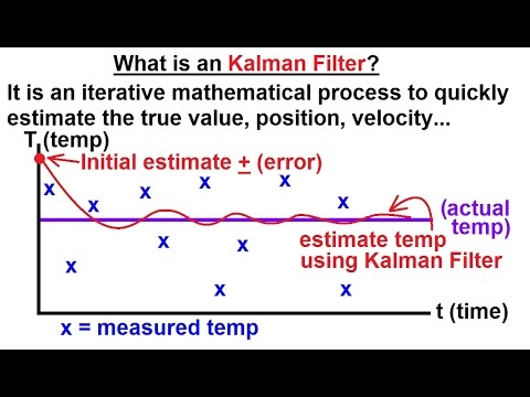
The filter's convergence is highly robust; even with an inaccurate initial guess, the algorithm rapidly drives the estimate toward the true value within just a few consecutive readings. (2:08)

Detailed notes

## Background Published on YouTube by Michel van Biezen on September 12, 2015, this video serves as the first installment in a multi-part series on the Kalman filter. The channel description notes that the video explains what the Kalman filter is and how it is used, directing viewers to ilectureonline.com for more math and science lectures.

## TL;DR This video introduces the Kalman filter as an iterative mathematical tool designed to estimate true values from noisy, uncertain measurements in real time. Unlike traditional statistical methods that require large historical datasets to calculate a reliable average, the Kalman filter updates step-by-step with each consecutive data input, rapidly converging on the true value. The filter can be applied to simple scalar measurements like temperature, as well as complex, multi-variable tracking systems like radar and GPS navigation that require matrix equations to simultaneously estimate position and velocity.

## Atmosphere & style The tone of the video is highly educational, encouraging, and structured, reflecting Michel van Biezen's clear and accessible teaching style. He acknowledges the inherent complexity of the subject upfront, easing the viewer's potential intimidation before systematically demystifying the concept with intuitive, real-world analogies. Watching the lecture feels like sitting in a supportive, well-paced classroom where complex mathematical theories are broken down into manageable, practical steps.

## Bulletin - [00:00](https://www.youtube.com/watch?v=CaCcOwJPytQ&t=0s) The Kalman filter is an iterative mathematical tool that estimates true values from noisy, uncertain measurements in real-time, eliminating the need to collect large historical datasets before calculating a reliable average. - [00:00](https://www.youtube.com/watch?v=CaCcOwJPytQ&t=0s) Unlike traditional statistical averaging, the Kalman filter begins converging almost immediately by evaluating each new input alongside its associated uncertainty or variation. - [02:08](https://www.youtube.com/watch?v=CaCcOwJPytQ&t=128s) While simple single-variable tracking (like temperature) can be solved with scalar equations, complex applications like radar and GPS tracking require matrix formulations to simultaneously estimate coupled variables like position and velocity. - [02:08](https://www.youtube.com/watch?v=CaCcOwJPytQ&t=128s) The filter's convergence is highly robust; even with an inaccurate initial guess, the algorithm rapidly drives the estimate toward the true value within just a few consecutive readings.

## Key takeaways - [00:00](https://www.youtube.com/watch?v=CaCcOwJPytQ&t=0s) The Kalman filter is a powerful mathematical tool designed to estimate predicted values from uncertain or noisy measurements. - [00:00](https://www.youtube.com/watch?v=CaCcOwJPytQ&t=0s) It operates as an iterative process, updating its estimate step-by-step as each new data input arrives. - [00:00](https://www.youtube.com/watch?v=CaCcOwJPytQ&t=0s) Traditional statistical methods require a large backlog of data points to calculate an accurate mean, whereas the Kalman filter does not wait for a large batch of inputs. - [00:00](https://www.youtube.com/watch?v=CaCcOwJPytQ&t=0s) The filter achieves rapid convergence by analyzing both the incoming data and the associated uncertainty or variation of those inputs. - [00:00](https://www.youtube.com/watch?v=CaCcOwJPytQ&t=0s) Raw sensor data inevitably contains random errors, unpredictability, and measurement noise, making direct interpretation difficult without filtering. - [00:00](https://www.youtube.com/watch?v=CaCcOwJPytQ&t=0s) The Kalman filter is highly versatile and can be applied to various physical properties, such as temperature, position, and velocity. - [02:08](https://www.youtube.com/watch?v=CaCcOwJPytQ&t=128s) In a simple scalar example like tracking temperature, the filter starts with an initial estimate and an initial estimate of error. - [02:08](https://www.youtube.com/watch?v=CaCcOwJPytQ&t=128s) The accuracy of the initial starting guess is not critical, as the algorithm quickly corrects and drives the estimate toward the true value. - [02:08](https://www.youtube.com/watch?v=CaCcOwJPytQ&t=128s) Within just a few consecutive readings, the variations in the filter's output shrink, tracking the true value with high precision. - [02:08](https://www.youtube.com/watch?v=CaCcOwJPytQ&t=128s) Single-variable systems rely on simple scalar equations, which serve as an intuitive starting point for learning the filter's logic. - [02:08](https://www.youtube.com/watch?v=CaCcOwJPytQ&t=128s) Real-world tracking applications, such as radar and GPS, must concurrently estimate multiple coupled variables like position (X, Y) and velocity (Vx, Vy). - [02:08](https://www.youtube.com/watch?v=CaCcOwJPytQ&t=128s) To handle multiple simultaneous data streams in navigation, the Kalman filter transitions from scalar arithmetic to matrix formulations. - [02:08](https://www.youtube.com/watch?v=CaCcOwJPytQ&t=128s) High-stakes tracking systems rely heavily on Kalman filtering because sensor noise cannot be entirely eliminated at the hardware level.

## Detailed walkthrough ### [00:00](https://www.youtube.com/watch?v=CaCcOwJPytQ&t=0s) Definition and the Core Iterative Process

Michel van Biezen introduces the Kalman filter as an extraordinary mathematical tool designed to estimate predicted values from uncertain measurements, acknowledging right away that it can often be quite difficult to grasp how it operates under the hood. At its core, the Kalman filter is an iterative mathematical process governed by a set of equations that work in tandem with consecutive data inputs arriving over time. Rather than waiting to collect an entire historical data set, the filter updates step by step: an input arrives, the equations compute an updated estimate, the next input arrives, another estimate is calculated, and the cycle continues.

```mermaid flowchart LR accTitle: Kalman Filter Iterative Loop accDescr: The cycle of receiving a noisy measurement, calculating an updated estimate via equations, and taking in the next input. A["Noisy Data Input"] --> B["Kalman Filter Equations"] B --> C["Updated True Value Estimate"] C -->|"Next time step"| A ```

Van Biezen contrasts this iterative approach with standard statistical methods, such as taking a batch of fifty or one hundred data points, plotting their distribution, and calculating the mean. While an average of many points will eventually get close to the truth, it demands an extensive backlog of data before offering a reliable answer. In contrast, the Kalman filter begins converging immediately by evaluating each input alongside its associated uncertainty or variation. As Michel van Biezen explains:

> “The Kalman filter doesn't wait for a whole bunch of inputs. It very quickly starts to narrow in to the true value by taking a few of those inputs and by on by understanding the variation or the uncertainty of those inputs, those data inputs.”

- The measured values fed into the filter inevitably contain random errors, unpredictability, and measurement noise rather than revealing the exact state directly. - The filter can be applied to diverse physical properties, including position, velocity, and temperature. - Because raw sensor data tends to bounce erratically, conventional systems struggle to deduce the true value rapidly without large sample sets.

---

[02:08](https://www.youtube.com/watch?v=CaCcOwJPytQ&t=128s) A Simple Temperature Example and Tracking Applications

To build an intuitive picture of how the filter behaves, van Biezen presents a simple scalar example: tracking ambient temperature with an inaccurate thermometer. On a graph where the vertical axis represents temperature and the horizontal axis tracks consecutive time samples, individual measurements bounce up and down across the plot due to sensor noise. Averaging these raw readings would take a long time to stabilize. The Kalman filter, however, begins with an initial estimate and an initial estimate of error or uncertainty—and the exact starting guess hardly matters. Within just a few incoming readings, the algorithm drives the estimate toward the actual value; as consecutive points arrive, variations shrink until the output tracks the true temperature with remarkable precision.

```mermaid flowchart TD accTitle: Scalar vs Matrix Tracking Systems accDescr: Progression from single-variable measurement to multi-variable matrix systems. subgraph Scalar["Single-Variable System"] S1["Thermometer Reading"] --> S2["Single-Equation Scalar Filter"] end subgraph Multi["Multi-Variable Tracking System"] M1["Radar / GPS Data"] --> M2["Matrix Equations"] M2 --> M3["Position (X, Y) & Velocity (Vx, Vy)"] end ```

While a single-variable measurement like temperature relies on simple scalar equations, real-world navigation and target tracking require simultaneous convergence of multiple coupled variables. Van Biezen points to radar tracking of aircraft or targets and GPS satellite positioning, where systems must concurrently determine position along the x-axis, position along the y-axis, velocity along the x-axis, and velocity along the y-axis. Tracking moving targets across air or space is far from an exact science, and sensor data is filled with significant noise and uncertainty. Handling these multiple simultaneous streams requires shifting from simple arithmetic equations to matrix formulations. As Michel van Biezen notes regarding the roadmap for the lecture series:

> “What that means is that when we track satellites or airplanes, we'll have to use instead of using a single number system and a simple set of equations, we'll have to use equations using, of course, matrices, and we'll show you how to do that as well.”

- Scalar models serve as the foundational starting point to master the core logic before moving to complex matrix mathematics. - High-stakes applications like radar and satellite tracking rely heavily on Kalman filtering because sensor noise cannot be completely eliminated at the hardware level. - The upcoming lectures are designed to move from concrete, worked-out numeric examples to multi-variable matrix tracking so learners develop a practical, hands-on intuition for applying the filter themselves.

## Video description Visit http://ilectureonline.com for more math and science lectures!

In this video I will explain what is Kalman filter and how is it used.

Next video in this series can be seen at: https://youtu.be/tk3OJjKTDnQ

[Source](https://www.youtube.com/watch?v=CaCcOwJPytQ)

中文简报

专题——卡尔曼滤波（第 1/55 集）什么是卡尔曼滤波？本视频介绍了卡尔曼滤波器，它是一种旨在实时从充满噪声且不确定的测量值中估计真实值的迭代数学工具。与需要海量历史数据来计算可靠平均值的传统统计方法不同，卡尔曼滤波器随着每个连续的数据输入逐步更新，从而快速收敛至真实值。该滤波器既可应用于像温度这样简单的标量测量，也能应用于雷达和 GPS 导航等复杂的的多变量跟踪系统，后者需要利用矩阵方程同时估计位置与速度。卡尔曼滤波器是一种迭代数学工具，可实时从充满噪声且不确定的测量值中估计真实值，无需在计算可靠平均值之前收集海量历史数据。 (0:00) 与传统的统计平均方法不同，卡尔曼滤波器通过结合每个新输入值及其相关的不确定性或方差进行评估，几乎能立即开始收敛。 (0:00) 虽然简单的单变量跟踪（如温度）可以用标量方程解决，但雷达和 GPS 跟踪等复杂应用则需要矩阵形式，以同时估计位置和速度等耦合变量。 (2:08) 该滤波器的收敛性非常稳健；即便初始猜测不准确，算法也能在短短几个连续读数内迅速推动估计值趋近真实值。 (2:08)

Reading summary

Michel van Biezen presents the Kalman filter as an iterative mathematical process designed to estimate true physical values from noisy, uncertain sensor measurements without requiring large batches of historical data. Iterative Updating Versus Batch Statistical Averaging (0:00) Standard statistical estimation typically relies on accumulating a substantial backlog of fifty to one hundred data points before plotting a distribution and calculating a mean. While this approach eventually approaches the true value, it introduces significant lag because the system must wait to collect a large dataset. In contrast, the Kalman filter functions as an iterative algorithm governed by equations that update step by step as consecutive measurements arrive. Rather than accumulating historical data, it computes an updated estimate immediately upon receiving each new input. Because raw sensor readings across physical metrics—such as position, velocity, and temperature—inevitably carry random errors, unpredictability, and hardware noise, direct measurement rarely reveals the exact state. Van Biezen explains that the Kalman filter converges rapidly by factoring in the variation and uncertainty of each incoming data point, allowing systems to deduce the underlying truth far more quickly than conventional batch averaging. Rapid Convergence in Scalar Temperature Tracking (2:08) To demonstrate the core logic, van Biezen uses the scalar example of measuring ambient temperature with an inaccurate thermometer. When individual readings are plotted over time, sensor noise causes the data to fluctuate erratically above and below the actual value. A standard average would require an extended run of readings to stabilize, but the Kalman filter begins converging almost immediately. The algorithm initiates with an initial estimate of the state alongside an initial estimate of uncertainty or error. Van Biezen emphasizes that the accuracy of these initial guesses is largely inconsequential. Within just a few incoming data points, the filter's mathematical updates compensate for the starting assumptions, shrinking output variations and steering the estimate toward the true ambient temperature. Multi-Variable Tracking and Matrix Formulations (2:08) While single-variable applications like temperature monitoring rely on basic scalar equations, high-stakes navigation and target tracking involve multiple coupled variables. Applications such as radar tracking of aircraft and GPS satellite positioning must simultaneously estimate coordinates and motion across multiple dimensions, specifically position along the x-axis, position along the y-axis, velocity along the x-axis, and velocity along the y-axis. Because physical sensor noise cannot be entirely eliminated at the hardware level, tracking moving targets in air or space requires processing multiple uncertain streams concurrently. To manage these coupled variables, the Kalman filter transitions from single-number arithmetic to matrix-based equations, maintaining real-time estimation across multidimensional states. Van Biezen structures the lecture series to build intuition through scalar, worked-out numeric examples before advancing to complex matrix models, providing the mathematical groundwork necessary to implement real-time tracking in noisy, multi-variable environments.

精炼阅读摘要

Michel van Biezen 指出，卡尔曼滤波器是一种通过迭代数学方程从充满噪声和不确定性的测量数据中估算系统真实状态的核心工具。与依赖大量样本累积的传统批处理统计方法不同，该算法通过结合每次输入的测量误差与不确定性，在极少的数据输入下即可迅速收敛到真实值。逐次迭代机制与传统统计的差异 (0:00) 卡尔曼滤波器的核心在于其步进式的迭代处理流程。当连续的时间序列数据输入时，该算法依靠一组数学方程式即时计算并更新当前的状态估计，随后等待下一个数据点进入并重复循环，而无需预先收集全部历史数据集。现实世界中的传感器测量值往往夹杂随机误差与不可预测的测量噪声，导致原始数据剧烈波动。 van Biezen 强调，传统的统计分析通常需要收集五十到一百个数据点来绘制分布曲线并计算平均值，这种方式需要庞大的数据积压才能提供可靠的结论。相比之下，卡尔曼滤波器无需等待大量数据，它直接解析单个输入及其内在的方差或不确定性，从最初几个输入点开始便能迅速缩小估计误差，适用于温度、位置和速度等多种物理量的动态推算。标量温度估计中的快速收敛特性 (2:08) 为直观展示其运算机制，van Biezen 提出了使用不精准温度计测量环境温度的标量示例。在以时间为横轴、温度为纵轴的坐标系中，传感器噪声导致读数持续上下跳动，仅依靠简单读数求和平均需要很长时间才能稳定。卡尔曼滤波器在运行初期仅需设定一个初始估计值以及相应的初始误差或不确定性估计。van Biezen 指出，初始猜测的具体数值对最终结果影响微弱，算法仅需接收几个连续读数，便能驱动估计值迅速贴近真实温度；随着后续数据持续输入，输出结果的波动显著缩小，能够以极高的精度持续跟踪真实温度。复杂目标追踪与矩阵方程演进 (2:08) 虽然温度监测等单变量系统可依赖简单的标量代数方程解决，但在雷达探测飞机或 GPS 卫星定位等真实导航场景中，工程系统必须同时确定多维耦合变量。这些变量通常包括水平与垂直方向的位置（X 轴与 Y 轴）以及对应的即时速度分量。在空中或太空追踪移动目标时，测量环境存在显著噪声，且硬件层面无法彻底消除传感器扰动。针对这种多数据流并行处理的需求，滤波体系必须从简单的标量算术升级为矩阵方程组。van Biezen 说明，该系列课程的规划旨在通过具体数值演算帮助学习者建立直观理解，随后逐步过渡到多变量矩阵形式，以解决现代雷达与卫星追踪中高度复杂的动态估计难题。该讲座确立了卡尔曼滤波器作为实时估算工具的基本定位，并论证了从单变量标量向多变量矩阵扩展的必要性；但作为导论内容，本讲尚未展开滤算法具体的代数推导、协方差更新步骤及参数赋值规则，相关数学实现留待后续课程逐一拆解。

Detailed notes — zh

## Background 本视频由知名理科讲师 Michel van Biezen 于 2015 年 9 月 12 日发布在 YouTube 频道，是其卡尔曼滤波器系列专题教学的第 1 集。视频简介指出，本期内容旨在向学习者通俗易懂地解释什么是卡尔曼滤波器以及它在实际工程中是如何应用的。 ## TL;DR 视频系统阐述了卡尔曼滤波器的基本数学原理与工程意义。与需要收集海量数据才能计算均值的传统统计方法不同，卡尔曼滤波器采用递推迭代的方式，每接收一个新测量值就实时更新一次估计，即使初始值并不准确，也能利用不确定性在极短时间内迅速收敛并逼近真实物理值。主讲人通过带有噪声的温度计读数直观演示了算法的平滑与抗干扰效果，并进一步指出在雷达与 GPS 追踪等涉及多维位置与速度的复杂场景中，该算法会从基础标量方程扩展为多维矩阵运算来协同解算状态。 ## Atmosphere & style 教学氛围沉稳而清晰，带有经典的大学黑板板书讲堂质感。讲师循序渐进、娓娓道来，巧妙地用平实直观的比喻化解了原本高深抽象的高等工程数学概念，整体节奏踏实笃定，给初学者带来一种由浅入深、豁然开朗的求知安心感。 ## Bulletin - [00:00](https://www.youtube.com/watch?v=CaCcOwJPytQ&t=0s) 卡尔曼滤波器是一种基于递推方程的数学迭代算法，专为应对传感器测量中的随机噪声与动态不确定性而设计。 - [00:00](https://www.youtube.com/watch?v=CaCcOwJPytQ&t=0s) 相较于需要预先收集数十或上百个数据点的传统平均统计法，卡尔曼滤波器仅需极少输入数据即可迅速收敛并锁定真实物理值。 - [02:08](https://www.youtube.com/watch?v=CaCcOwJPytQ&t=128s) 该算法对初始状态猜测具备极高容错率，即使初始估计值不准，也能结合误差范围在几轮迭代内完成自主修正。 - [03:41](https://www.youtube.com/watch?v=CaCcOwJPytQ&t=221s) 面对雷达追踪与GPS导航等高维复杂系统，卡尔曼滤波器通过拓展为矩阵方程组，实现对物体位置与速度多维状态的同步解算。 ## Key takeaways - [00:00](https://www.youtube.com/watch?v=CaCcOwJPytQ&t=0s) 卡尔曼滤波器是工程与科学测量中估计真实状态的关键工具，但其数学机制对初学者而言往往较为晦涩。 - [00:00](https://www.youtube.com/watch?v=CaCcOwJPytQ&t=0s) 算法本质上是一个递推式迭代计算过程，每接收一个新数据点便更新一次状态估计，无需进行离线批量处理。 - [00:00](https://www.youtube.com/watch?v=CaCcOwJPytQ&t=0s) 传统统计学依赖收集50到100个采样点绘制概率分布求均值，这种滞后处理模式无法满足实时系统的需求。 - [00:00](https://www.youtube.com/watch?v=CaCcOwJPytQ&t=0s) 真实世界的传感器读数往往受到未预测噪声和扰动的影响，导致测量值在真实物理量周围剧烈波动。 - [00:00](https://www.youtube.com/watch?v=CaCcOwJPytQ&t=0s) 卡尔曼滤波器通过量化并结合输入数据的方差与不确定性，在极少的数据采样点内迅速逼近真实值。 - [02:08](https://www.youtube.com/watch?v=CaCcOwJPytQ&t=128s) 在单变量温度测量案例中，算法启动时的初始估计数值并不关键，核心在于设定与之对应的不确定度或误差范围。 - [02:08](https://www.youtube.com/watch?v=CaCcOwJPytQ&t=128s) 随着测量序列展开，卡尔曼滤波计算出的估计轨迹能够在极短时间内跨越偏差并向真实温度收敛。 - [02:08](https://www.youtube.com/watch?v=CaCcOwJPytQ&t=128s) 进入收敛状态后，滤波输出的方差显著收窄，即使传感器输入依然大幅跳跃，估计值仍能稳固锁定在极小波动区间内。 - [03:41](https://www.youtube.com/watch?v=CaCcOwJPytQ&t=221s) 单标量测量主要用于直观理解算法逻辑，而在实际航天、航空与导航应用中，系统通常需要面对多维状态追踪。 - [03:41](https://www.youtube.com/watch?v=CaCcOwJPytQ&t=221s) 雷达与GPS系统必须在噪声干扰下，同步解算目标在多维空间中的坐标位置（X、Y轴）以及即时运动速度（X、Y轴速度）。 - [03:41](https://www.youtube.com/watch?v=CaCcOwJPytQ&t=221s) 为了处理多个耦合变量的同时收敛，卡尔曼滤波器的数学表达必须从简单的标量代数演进为矩阵方程组计算。 - [03:41](https://www.youtube.com/watch?v=CaCcOwJPytQ&t=221s) 从直观的单变量温度计实例逐步过渡到多维状态空间矩阵运算，是掌握复杂卡尔曼滤波工程应用的核心路径。 ## Detailed walkthrough ### [00:00](https://www.youtube.com/watch?v=CaCcOwJPytQ&t=0s) 卡尔曼滤波器的基本概念与迭代机制在工程与科学测量领域，卡尔曼滤波器是一个极具价值的核心算法。Michel van Biezen 解释说，尽管它在预测和估计真实状态方面表现优异，但其内在运行机制往往让初学者感到晦涩难懂。正如 Michel van Biezen 所指出的：“Now, the Kalman filter is an amazing tool in order to estimate predicted values, but it's sometimes very difficult to understand how the Kalman filter actually works.” 本质上，卡尔曼滤波器是一个迭代式的数学处理过程。它依托一组明确的数学方程，逐步接收连续输入的数据。每当系统接收到一个新的测量数据点，就会代入公式并计算出最新的估计值；紧接着，下一个数据点传入，系统再基于前一次的结果计算出更新的估计值。这种递推式的计算方式旨在以极快的速度逼近被测对象的真实物理值。通常情况下，若收集到 50 或 100 个测量数据，人们会习惯于先绘制这些数值的概率分布并计算平均值，以此推断真实值。但这种传统统计方法存在严重滞后，必须预先收集大量数据才能展开计算。卡尔曼滤波器则截然不同，它完全无需等待海量数据就位，而是从最开始的几个输入点出发，通过量化和利用输入数据本身的方差与不确定性，在极短时间内锁定真实值。真实世界的传感器往往受到未预测噪声、随机误差及扰动的干扰，导致单次读数在真实值周围大幅跳动，而卡尔曼滤波器恰好专为处理这种充满不确定性的动态测量而设计。 ```mermaid flowchart LR accTitle: 卡尔曼滤波器单步迭代循环 accDescr: 展示数据输入、状态估计与连续迭代的递推过程 subgraph Iteration["单步递推过程"] A["新测量数据输入"] --> B["代入数学方程计算"] B --> C["更新当前状态估计"] C -->|"结合不确定性进入下一轮"| A end ``` - 核心属性：基于方程组的递推数学迭代过程，无需离线批量处理全部数据。 - 适用对象：物理位置、移动速度、温度等含有随机误差或未预测波动的测量目标。 - 核心优势：能够结合测量的不确定性，在极少的数据采样点内迅速收敛至真实值。 ### [02:08](https://www.youtube.com/watch?v=CaCcOwJPytQ&t=128s) 温度测量实例：从初始估计到逼近真实值为了以直观的可视化方式展现卡尔曼滤波器的运作方式，Michel van Biezen 举了一个测量温度的具体案例。假设使用一支精度较差的温度计进行连续采样，坐标系纵轴代表测量温度，横轴代表时间序列或连续的采样点。由于测量工具的不确定性与各种噪声影响，采集到的各数据点在图表上呈现上下跳动的交叉点，波动幅度极大。如果仅靠常规的长时间平均法，系统需要等待非常久的时间才能得出可靠结论。卡尔曼滤波器的计算流程始于一个初始估计值。令人惊讶的是，这个初始值具体是多少其实并不重要，只需为其设定一个对应的不确定度或预期误差范围即可。随着后续数据点逐个传入并进入迭代环节，卡尔曼滤波器的预测轨迹会迅速向真实温度靠拢。正如下述结论所强调的，Michel van Biezen 表示：“So, the estimated temperature using the Kalman filter will zero in and come very, very close to the actual temperature very quickly.” 一旦进入收敛区间，随着更多采样数据不断累积，卡尔曼滤波器计算出的数值波动会变得微乎其微。即使后续输入的原始传感器数据依然四处跳跃，滤波器给出的估计值依然能稳固锁定在极度贴近真实温度的狭窄范围内，展现出强大的噪声抑制与状态追踪能力。 - 初始容错率高：初始估计值无需绝对精准，算法具备自主修正并快速向真实值靠拢的特性。 - 收敛速度快：仅需少量采样点即可消除初期的较大偏差，极大缩短了响应时间。 - 稳定性高：完成初始收敛后，后续计算值的方差显著收窄，输出表现出高平滑度与抗干扰性。 ### [03:41](https://www.youtube.com/watch?v=CaCcOwJPytQ&t=221s) 拓展到多维系统：雷达与 GPS 追踪中的矩阵运算单变量的温度测量只是理解卡尔曼滤波器的切入点。在雷达追踪系统和 GPS 卫星导航等尖端工程应用中，待测对象往往具有多维度的物理状态。例如，追踪高空飞行器或卫星轨道时，系统必须同时确定其在 X 轴方向的位置、Y 轴方向的位置、X 轴方向的速度以及 Y 轴方向的速度。通过雷达捕捉空中目标或借助卫星信号定位并非精密无误的绝对测量，原始数据中充斥着复杂的空间不确定性与噪声。面对离散跳跃的多维采样，卡尔曼滤波器依然能够通过相同的底层逻辑，从混乱的数据流中提取出物体的真实轨迹与即时速度。然而，处理多个需要同时收敛的耦合变量，其复杂度远超温度计的标量计算。正如 Michel van Biezen 解释技术演进时所说：“What that means is that when we track satellites or airplanes, we'll have to use instead of using a single number system and a simple set of equations, we'll have to use equations using, of course, matrices, and we'll show you how to do that as well.” 对于这种复杂的多维追踪问题，标量计算必须扩展为矩阵方程组的形式。整个系列教学的推进路径也由此确立：先从最直观的单变量温度计实例入手，帮助学习者建立对误差协方差与递推逼近的直观感知；在此基础上，进一步将数学工具拓展为多维矩阵状态空间方程，从而彻底掌握雷达目标捕捉与卫星定位等复杂场景下的卡尔曼滤波应用。 - 多维状态追踪：广泛应用于雷达与卫星导航，需同步解算位置向量（如 X、Y 坐标）与速度向量（如 X、Y 轴速度）。 - 数学表达演进：从简单的标量单一方程过渡为多变量矩阵运算，以适应多维数据同时收敛的需求。 - 学习进阶逻辑：先通过单标量温度测量理清概念骨架，再深入多维矩阵的工程计算细节。 ## Notable quotes > [00:00](https://www.youtube.com/watch?v=CaCcOwJPytQ&t=0s) Now, the Kalman filter is an amazing tool in order to estimate predicted values, but it's sometimes very difficult to understand how the Kalman filter actually works. — Michel van Biezen ## Mentioned Michel van Biezen, Kalman filter, GPS ## Video description Visit http://ilectureonline.com for more math and science lectures! In this video I will explain what is Kalman filter and how is it used. Next video in this series can be seen at: https://youtu.be/tk3OJjKTDnQ [Source](https://www.youtube.com/watch?v=CaCcOwJPytQ)

Source quotes

[0:00] Michel van Biezen: Now, the Kalman filter is an amazing tool in order to estimate predicted values, but it's sometimes very difficult to understand how the Kalman filter actually works.

Original transcript

[0:00] Welcome to Electron Academy, and in this [0:02] series of videos starting with this one, [0:04] we're going to talk about the Kalman [0:06] filter. Now, the Kalman filter is an [0:08] amazing tool in order to estimate [0:11] predicted values, but it's sometimes [0:14] very difficult to understand how the [0:15] Kalman filter actually works. So, [0:17] therefore, I made some videos to [0:19] describe what a Kalman filter actually [0:21] is, how to use it with some nice [0:23] examples. So, follow this. [0:25] So, what is a Kalman filter? Well, it is [0:28] an iterative mathematical process. It's [0:31] so you you follow a set of iterations. [0:34] It's a mathematical process that uses a [0:36] set of equations. Those equations and [0:39] consecutive data input. So, we get a [0:41] data input, we use the equation, we [0:43] calculate the new estimate, we get [0:45] another data input, we calculate the new [0:46] estimate, we get another data input, we [0:49] calculate the new estimate again. It's [0:50] an iterative process, [0:53] and the reason for doing it like this is [0:54] so that we can quickly estimate the true [0:57] value. [0:59] So, let's say that we have 50 or 100 [1:01] data points that come in one at a time. [1:04] And yeah, you could you And yes, we can [1:06] do a for example, a distribution of [1:09] these values and find the average value, [1:11] and then say, "Well, the average value [1:13] must be very close to the true value." [1:15] But in order to do that, we need to have [1:16] a whole bunch of inputs already. [1:19] The Kalman filter doesn't wait for a [1:21] whole bunch of inputs. It very quickly [1:23] starts to narrow in to the true value by [1:26] taking a few of those inputs and by on [1:28] by understanding the variation or the [1:31] uncertainty of those inputs, those data [1:33] inputs. So, it quickly estimates the [1:36] true value, position, velocity, whatever [1:39] it is that we're trying to measure of [1:41] the object that's being measured when [1:44] the measured values contain unpredicted [1:46] or random errors, uncertainties, or [1:48] variations as well. So, remember that [1:51] the data coming in is not the true [1:53] value, it's somewhere around the true [1:55] value with a certain amount of [1:56] uncertainty. And of course, since that [1:58] can bounce all over the place, it would [2:00] very difficult through any other system [2:02] to try and very figure out what the true [2:04] value is or come very close to the true [2:06] value. So, a very simple example here, [2:09] in the graphical sense, can help you [2:11] understand that. Let's say we're trying [2:13] to measure the temperature with a [2:14] certain thermometer. That thermometer is [2:17] not very accurate. It have a certain [2:19] amount of uncertainty in the data [2:20] measurements. [2:22] Let's say that the vertical axis here [2:24] means temperature, the horizontal axis [2:26] means time or consecutive sample inputs. [2:31] The little crosses here are consecutive [2:33] inputs. So, here the temperature is [2:35] measured to be this high, then to be [2:37] this high, to be this high, to be this [2:39] high, then this. So, you can see that [2:40] the temperature measured, time and [2:42] again, always varies because there's [2:44] certain amount of uncertainty in that [2:45] temperature measurement technique, for [2:47] whatever reason it may be. And so, [2:49] therefore, it would take a very long [2:51] time for us to average these values out. [2:54] The Kalman filter can do it a lot [2:55] faster. It starts out by taking an [2:57] initial estimate. It almost doesn't [2:59] matter what that initial estimate is. [3:01] And of course, in your estimate, you [3:03] have to predict a certain amount of [3:05] error or uncertainty. [3:07] But very quickly, as data points start [3:09] coming in and we go through that [3:11] iterative process, the Kalman filter [3:13] actually narrows down to somewhere close [3:16] to the true value very quickly. It [3:18] doesn't take very many data points to [3:19] get there. And once you get there, as [3:22] more and more data points come in, the [3:24] variations will become very, very small [3:26] and the predicted value through the [3:28] Kalman filter process will be very, very [3:31] close to the actual temperature in this [3:32] case, in this example. So, the estimated [3:35] temperature using the Kalman filter will [3:37] zero in and come very, very close to the [3:39] actual temperature very quickly. Now, in [3:42] this example here, there's only one [3:44] measured value we're after, the [3:46] temperature. However, this can be used, [3:48] especially like in radar technology or [3:51] GPS tracking satellites, we need to know [3:54] the target that we're tracking. We need [3:56] to know its position in the X direction, [3:57] the position in the Y direction, the [3:59] velocity in the X direction, the [4:01] velocity in the Y direction, and yes, [4:02] the common filter can very quickly again [4:05] to the very same process narrow down [4:08] narrow these intermediate values that [4:10] come in, which can be all over the place [4:11] because as you're trying to track [4:13] airplanes via radar or target via radar, [4:16] you're trying to track satellites, [4:17] that's not an exact science. The data [4:19] coming in will have certain amount of [4:21] uncertainty in it, and the common filter [4:23] can very easily handle that uncertainty [4:26] and very quickly zero in on the true [4:28] position and the true velocity of the of [4:30] the object that you're tracking. Of [4:32] course, if we're looking for something [4:33] like this where we have multiple data [4:35] inputs that we have to converge at the [4:38] same time, it's a little different [4:40] process than if we take a singular value [4:42] like the temperature measured with a [4:44] thermometer. [4:46] What that means is that when we track [4:48] satellites or airplanes, we'll have to [4:51] use instead of using a single number [4:52] system and a simple set of equations, [4:54] we'll have to use equations using, of [4:57] course, matrices, and we'll show you how [4:59] to do that as well. But to get the [5:01] technique down first, we're going to [5:03] start with a very simple example like [5:05] this, just simply measuring the [5:06] temperature, and see how Kalman filter [5:09] can very quickly zoom in to that actual [5:11] temperature that we're trying to figure [5:13] out. And then once we have that [5:15] technique down, then we'll expand it to [5:16] more complicated set of equations to be [5:19] used to figure out how to track targets [5:21] like using radar or how to use GPS [5:24] tracking, you know, tracking of [5:26] satellites. All right, hopefully that [5:28] gives you kind of an idea what a Kalman [5:29] filter is. Of course, without showing [5:31] examples, you're still a long ways [5:34] probably from saying, "Oh, okay, I'm [5:36] good with that. I know what this is." At [5:37] least you have a conceptual idea of what [5:39] a Kalman filter is. Now, let's go [5:42] practice with some real examples of how [5:44] to do that so you get a very strong feel [5:46] for what Kalman filters is and how to [5:48] use it yourself.