Pi Approximations Form Prime Spirals as Dirichlet Limits Residues
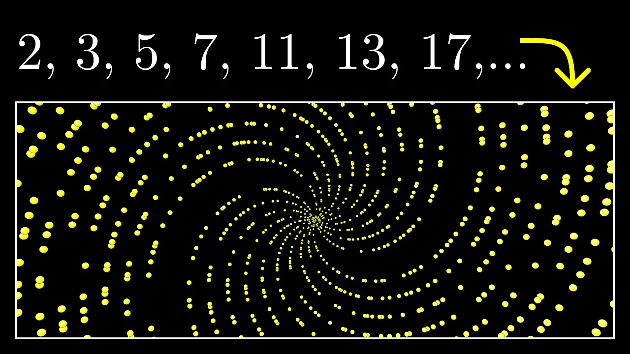
Why do prime numbers make these spirals? | Dirichlet’s theorem and pi approximations — 3Blue1Brown

3Blue1Brown

The galactic patterns seen in polar prime plots stem entirely from rational approximations of pi, which produce integer arms that prime numbers thin out equally across allowable residue classes.

AI-assisted summary of Why do prime numbers make these spirals? | Dirichlet’s theorem and pi approximations — original source. Check the original for full context.

Source published:

Key ideas

  • Plotting prime numbers in polar coordinates as (p, p) produces sweeping galactic spirals and radiating rays driven by rational approximations to 2π rather than intrinsic symmetries of the primes themselves. (0:03)
  • The 20 visible galactic spirals and 280 outer rays correspond directly to Euler's totient values φ(44) = 20 and φ(710) = 280, reflecting allowable residue classes coprime to the moduli 44 and 710. (7:20)
  • The straightness of the 280 outer rays provides a visual demonstration of how tightly 355/113 approximates π, corresponding to 710 radians equaling roughly 113.000095 full revolutions. (11:19)
  • Primes distribute asymptotically equally across coprime residue classes modulo n with limiting proportion 1/φ(n), connecting visual arm density directly to Dirichlet's theorem on arithmetic progressions. (16:45)

Detailed notes

## Background Published on YouTube by Grant Sanderson on the 3Blue1Brown channel on October 8, 2019, this video investigates a curious visual pattern of spiral arms and radiating rays that emerges when prime numbers are plotted in polar coordinates. The presentation explores the underlying mechanics behind the phenomenon, tying it to rational approximations of pi, residue classes, Euler's totient function, and Dirichlet's theorem on arithmetic progressions.

## TL;DR When numbers are plotted in polar coordinates as $(n, n)$ in radians, integer steps align into curving spirals and straight rays due to exceptionally close rational approximations of $2\pi$, specifically $44/7$ and $710/113$. Restricting the plot to prime numbers acts as a filter, wiping out residue classes that share prime factors with the modulus and leaving behind exactly $\phi(n)$ arms or rays as determined by Euler's totient function. Dirichlet's theorem accounts for why the surviving arms appear equally dense, establishing that primes distribute evenly across all allowable coprime residue classes. Through this visual puzzle, the video demonstrates how recreational mathematical play and data visualization can organically lead to deep principles in analytic number theory.

## Atmosphere & style The presentation carries 3Blue1Brown's signature calm, elegant, and intellectually generous tone, pairing hypnotic Manim animations with thoughtful, measured narration. It begins in an engaging playground of graphical curiosity, gently dismantles the illusion of prime mysticism with straightforward modular arithmetic, and gradually deepens into rigorous historical mathematics. Watching it feels like embarking on a collaborative detective story that moves from casual aesthetic wonder to a profound appreciation for mathematical rediscovery.

## Bulletin - [00:03](https://www.youtube.com/watch?v=EK32jo7i5LQ&t=3s) Plotting prime numbers in polar coordinates as (p, p) produces sweeping galactic spirals and radiating rays driven by rational approximations to 2π rather than intrinsic symmetries of the primes themselves. - [07:20](https://www.youtube.com/watch?v=EK32jo7i5LQ&t=440s) The 20 visible galactic spirals and 280 outer rays correspond directly to Euler's totient values φ(44) = 20 and φ(710) = 280, reflecting allowable residue classes coprime to the moduli 44 and 710. - [11:19](https://www.youtube.com/watch?v=EK32jo7i5LQ&t=679s) The straightness of the 280 outer rays provides a visual demonstration of how tightly 355/113 approximates π, corresponding to 710 radians equaling roughly 113.000095 full revolutions. - [16:45](https://www.youtube.com/watch?v=EK32jo7i5LQ&t=1005s) Primes distribute asymptotically equally across coprime residue classes modulo n with limiting proportion 1/φ(n), connecting visual arm density directly to Dirichlet's theorem on arithmetic progressions.

## Key takeaways - [00:03](https://www.youtube.com/watch?v=EK32jo7i5LQ&t=3s) Plotting points (n, n) in polar coordinates uses distance r = n and angle θ = n radians, tracing out a basic Archimedean spiral step by step. - [02:30](https://www.youtube.com/watch?v=EK32jo7i5LQ&t=150s) When restricted to primes, small scales appear chaotic, but large scales reveal 20 sweeping spiral arms and an even larger fan of 280 straight rays. - [03:35](https://www.youtube.com/watch?v=EK32jo7i5LQ&t=215s) The underlying spiral structures are not unique to primes; plotting all integers produces 44 cleaner spiral arms based on multiples of rational approximations. - [04:15](https://www.youtube.com/watch?v=EK32jo7i5LQ&t=255s) At the center, 6 arms emerge because 6 radians is slightly less than one full turn (2π ≈ 6.28318 radians), grouping numbers by residue classes modulo 6. - [05:30](https://www.youtube.com/watch?v=EK32jo7i5LQ&t=330s) Primes greater than 3 leave remainders of only 1 or 5 modulo 6, eliminating 4 of the 6 central arms and leaving only 2 active spirals. - [07:20](https://www.youtube.com/watch?v=EK32jo7i5LQ&t=440s) The 44-arm spiral pattern reflects the rational approximation 44/7 ≈ 2π (or 22/7 ≈ π), where advancing 44 radians equals roughly 7.0028 full revolutions. - [08:30](https://www.youtube.com/watch?v=EK32jo7i5LQ&t=510s) Filtering modulo 44 for primes removes all 22 even residue classes and 2 odd multiples of 11, leaving exactly φ(44) = 20 visible galactic arms. - [11:19](https://www.youtube.com/watch?v=EK32jo7i5LQ&t=679s) At broader scales, 710 radians corresponds to approximately 113.000095 full revolutions, corresponding to the exceptionally tight approximation 355/113 ≈ π. - [12:20](https://www.youtube.com/watch?v=EK32jo7i5LQ&t=740s) Because 710 steps advance by nearly an exact integer number of turns, sequences of residue classes modulo 710 appear as nearly straight radial lines. - [12:59](https://www.youtube.com/watch?v=EK32jo7i5LQ&t=779s) Factoring 710 into 2 × 5 × 71 explains why prime rays group into clusters of four (from removing multiples of 5) with periodic missing teeth (from multiples of 71). - [14:05](https://www.youtube.com/watch?v=EK32jo7i5LQ&t=845s) The number of remaining prime rays equals φ(710) = 280, the count of positive integers up to 710 coprime to 710. - [14:38](https://www.youtube.com/watch?v=EK32jo7i5LQ&t=878s) In base 10, primes greater than 5 must end in 1, 3, 7, or 9, with primes dividing asymptotically equally among these four allowable terminal digits at 25% each. - [16:45](https://www.youtube.com/watch?v=EK32jo7i5LQ&t=1005s) In general, the proportion of primes up to x in any allowable residue class modulo n approaches 1/φ(n) as x approaches infinity. - [18:20](https://www.youtube.com/watch?v=EK32jo7i5LQ&t=1100s) Dirichlet proved in 1837 that arithmetic progressions coprime to their step size contain infinitely many primes, introducing complex analysis to number theory. - [20:17](https://www.youtube.com/watch?v=EK32jo7i5LQ&t=1217s) Reinventing mathematical concepts through playful visual experimentation provides intuitive grounding that makes formal definitions feel natural rather than arbitrary.

## Detailed walkthrough ### [00:03](https://www.youtube.com/watch?v=EK32jo7i5LQ&t=3s) The Polar Coordinate Setup and the Spiral Mystery

The visual puzzle originated on Math Stack Exchange from a user named Dwymark, who posed a question about a peculiar pattern that emerged when visualizing primes, answered by Greg Martin. It ties together the distribution of prime numbers with rational approximations for $\pi$. The underlying experiment involves plotting points in two-dimensional polar coordinates $(r, \theta)$. Unlike familiar Cartesian $(x, y)$ coordinates, polar coordinates define a point by its radial distance $r$ from the origin and an angle $\theta$ measured counterclockwise from the positive horizontal axis. Angles are expressed in radians, meaning an angle of $\pi$ represents a half turn and $2\pi$ represents a full circle. Because angles wrap around every $2\pi$, polar coordinates are not unique; shifting an angle by any multiple of $2\pi$ points to the exact same position in space.

```mermaid flowchart TD accTitle: Polar coordinate point generation accDescr: Progression of points mapped with polar coordinates (n, n) in radians and distance. subgraph Progression["Iterative plotting of (n, n)"] P1["Point (1, 1)<br/>r = 1, θ = 1 rad"] --> P2["Point (2, 2)<br/>r = 2, θ = 2 rad"] P2 --> P3["Point (3, 3)<br/>r = 3, θ = 3 rad<br/>(θ just under π)"] P3 --> PN["General Point (n, n)<br/>r = n, θ = n rad"] end PN --> Spiral["Archimedean Spiral<br/>r = θ"] ```

The construction consists of plotting points where both coordinates are set to the exact same value: $(p, p)$ for every prime number $p$. As Grant Sanderson explains: “There is no practical reason to do this, it's purely fun, we're just frolicking around in the playground of data visualization.” To see how the geometry behaves, consider plotting all whole numbers $(n, n)$ rather than only the primes: - The point $(1, 1)$ sits at a radius of $1$ at an angle of $1$ radian, which means the subtended circular arc along the unit circle equals the radial line's length. - The point $(2, 2)$ doubles both the radial distance and the angle ($2$ radians). - The point $(3, 3)$ steps out to a distance of $3$ at $3$ radians—just shy of a straight half-turn, since $3$ is slightly less than $\pi \approx 3.14159$.

Step by step, the process resembles the tip of an expanding clock hand that advances by one radian per tick (a bit under a sixth of a complete turn) while growing outward by one unit with each step. This trace generates a classic Archimedean spiral. When you drop all composite numbers and plot only the primes, the small-scale picture looks chaotic and unpredictable. Zooming out, however, reveals an organized structure: sweeping, galactic-looking spiral arms with noticeable gaps where certain arms seem to have vanished entirely. Zooming out even further, the swirling arms straighten out into a massive fan of distinct, outwardly radiating rays. These rays often appear in clusters of four, interrupted by missing slots like a comb with broken teeth. Patiently counting the features at each scale reveals exactly 20 visible galactic spiral arms and, further out, a total of 280 straight rays.

[03:35](https://www.youtube.com/watch?v=EK32jo7i5LQ&t=215s) Demystifying the Spirals via Whole Numbers and Modulo 6

While such structure tempts one to assume a mystical, hidden symmetry within the primes, the premise is somewhat misleading. If you repeat the experiment with *all* positive integers rather than just prime numbers, the exact same galactic spirals appear. Without the prime filter, the pattern is far cleaner and contains 44 spiral arms instead of 20. Thus, the physical origin of the spirals is completely divorced from prime numbers; it is purely an artifact of rational approximations to $2\pi$. The role of the primes is strictly that of a filter, carving out gaps and thinning the arms. Yet answering why certain arms survive and others vanish connects directly to Dirichlet’s theorem on arithmetic progressions.

To see why the integer plot forms spirals at all, look at the very center of the diagram, where a family of 6 smaller spirals emerges: - One arm consists entirely of the multiples of 6: $\{0, 6, 12, 18, \dots\}$. - The adjacent arm contains the numbers that are 1 above a multiple of 6: $\{1, 7, 13, 19, \dots\}$. - Subsequent arms correspond to numbers that are 2 above, 3 above, 4 above, and 5 above a multiple of 6.

Because each integer steps forward by 1 radian, jumping forward by 6 integers corresponds to a rotation of 6 radians. A full circle is $2\pi \approx 6.28318$ radians, so 6 radians falls just short of a full turn. Every time you add 6, the pointer sweeps around almost a full turn, ending at an angle slightly smaller than where it started. Repeating this step places each successive multiple of 6 just behind the previous one at an ever-increasing radius, creating the smooth visual illusion of a gently curving spiral arm.

When restricted to prime numbers, 4 of these 6 arms vanish entirely, leaving only 2: - Numbers that are multiples of 6 cannot be prime. - Numbers that are 2 above or 4 above a multiple of 6 are even, making them composite (with the sole exception of the prime 2). - Numbers that are 3 above a multiple of 6 are multiples of 3, making them composite (with the sole exception of the prime 3). - Consequently, all primes larger than 3 must leave a remainder of either 1 or 5 when divided by 6, populating only two surviving spiral arms.

In the formal language of mathematics, each sequence generated by stepping by 6 is termed a residue class modulo 6. As Sanderson quips, “The word residue here is sort of an overdramatic way of saying remainder, and mod means something like where the thing you divide by is.” Saying that 20 has a residue of 2 mod 6 is merely a pretentious way to say that dividing 20 by 6 leaves a remainder of 2.

[07:20](https://www.youtube.com/watch?v=EK32jo7i5LQ&t=440s) The 44-Arm Galactic Spirals and Euler’s Totient Function

The larger galactic spiral pattern operates on the exact same mechanism, substituting 44 for 6. While 6 radians is roughly a single rotation, stepping forward by 44 radians produces:

$$\frac{44}{2\pi} \approx 7.0028 \text{ full turns}$$

This value is exceptionally close to 7 full rotations, meaning 44 steps brings you slightly past 7 full circles. This reflects the familiar rational approximation:

$$\frac{44}{7} \approx 2\pi \quad \iff \quad \frac{22}{7} \approx \pi$$

Because 44 radians is just a tiny fraction greater than 7 full turns, adding 44 lands at nearly the same angular direction, nudged just slightly counterclockwise. As radius increases by 44 with each step, the sequence of points $\{0, 44, 88, 132, \dots\}$ traces out an extremely gentle, slowly curving spiral arm. Offsetting the start by 1 gives the residue class of numbers 1 above a multiple of 44, rotated by 1 radian counterclockwise. Doing this for every offset from 0 to 43 produces 44 clean spiral arms representing every residue class modulo 44.

When filtering for primes, many arms disappear: - Any residue class consisting of even numbers (offsets 0, 2, 4,..., 42) contains only composites (except for the prime 2), wiping out 22 arms. - Offsets sharing a factor of 11 with 44—specifically 11, 22, and 33—contain only multiples of 11 (with 11 itself being the only prime), wiping out the remaining odd multiples of 11.

```mermaid flowchart LR accTitle: Filtering residue classes mod 44 for primes accDescr: Breakdown of the 44 total residue classes mod 44 into composite-dominated classes and coprime surviving classes. Total["44 Residue Classes<br/>mod 44"] --> Evens["22 Even Classes<br/>(offsets 0, 2,..., 42)<br/>Contain no primes > 2"] Total --> Mult11["2 Odd Multiples of 11<br/>(offsets 11, 33)<br/>Contain no primes > 11"] Total --> Coprimes["20 Coprime Classes<br/>gcd(a, 44) = 1<br/>ϕ(44) = 20"] Coprimes --> Visible["20 Visible Prime<br/>Galactic Spirals"] ```

The only spiral arms that remain visible are those corresponding to residue classes whose offsets share no prime factors with 44 (that is, offsets not divisible by 2 or 11). Two numbers that share no common factors other than 1 are called relatively prime, or coprime.

Counting the integers between 1 and 44 that are coprime to 44 yields exactly 20 numbers: - 1, 3, 5, 7, 9, 13, 15, 17, 19, 21, 23, 25, 27, 29, 31, 35, 37, 39, 41, 43.

In number theory, this count is written compactly as $\phi(44) = 20$, where $\phi$ denotes Euler’s totient function. As Sanderson highlights: “More obscurely, and I had never heard this before but I find it too delightful not to tell, these numbers are sometimes called the totitives of n.”

The image observed on Math Stack Exchange is therefore the intersection of two distinct mathematical phenomena: 1. The fraction $44/7$ serves as an extraordinarily tight rational approximation for $2\pi$, organizing the integers into 44 distinct geometric spirals. 2. Filtering by prime numbers eliminates the 24 residue classes that share common factors with 44, leaving behind exactly $\phi(44) = 20$ arms where primes are free to appear infinitely often.

[10:28](https://www.youtube.com/watch?v=EK32jo7i5LQ&t=628s) Transition to the Larger Scale

Just as 6 radians approximates 1 full turn, and 44 radians approximates 7 full turns, stepping out to even broader scales reveals why straight rays emerge instead of curving spirals. At that vast scale, the points align because 710 radians happens to land almost precisely on a whole number of full revolutions. Visually, this alignment causes the plotted point at 710 to strike almost dead-on along the positive $x$-axis, setting the stage for an analytical breakdown of higher-order rational approximations to $\pi$.

[11:19](https://www.youtube.com/watch?v=EK32jo7i5LQ&t=679s) The 710 Radians Approximation and Pi

710 radians evaluates to $710 / 2\pi$ complete revolutions, which equals approximately $113.000095$ full turns. This corresponds to the rational fraction $710/113$ being an exceptionally close approximation of $2\pi$, or in its more familiar reduced form, $355/113 \approx \pi$. That fraction provides an unusually precise rational estimate for $\pi$—far more accurate than comparable approximations achievable for other fundamental mathematical constants such as $\phi$, $e$, or $\sqrt{2}$.

Because $710$ radians is almost an exact whole number of full revolutions ($113$ full turns plus just under one ten-thousandth of a turn), moving outward in steps of $710$ produces points whose polar angles match almost perfectly with the previous point, shifting by only an imperceptible fraction of an angle. Outward sequences along these residue classes modulo $710$ appear as straight radial lines across large scales. Rendering all 710 individual residue classes simultaneously overwhelms standard screen resolutions, packing them into an indistinguishable cloud. Restricting the visualization strictly to prime numbers removes most of these classes and makes the individual rays visible. At sufficiently high magnification, a gentle curvature becomes discernible; as Grant Sanderson notes, “the fact that it takes so long to become prominent is a wonderful illustration, maybe the best illustration I've ever seen, for just how good an approximation this is for 2 pi.”

- $710 / 2\pi \approx 113.000095$ rotations. - Ratio $710/113 \approx 2\pi$ reduces to $355/113 \approx \pi$. - Recommended reference for rational approximations: Mathologer's video on continued fractions and approximations.

---

[12:59](https://www.youtube.com/watch?v=EK32jo7i5LQ&t=779s) Residue Classes Modulo 710 and Prime Rays

The mechanism behind the ray patterns seen modulo $710$ matches the mechanics seen modulo $44$. The prime factorization of $710$ is $2 \times 5 \times 71$. Any residue class sharing one of these prime factors cannot contain primes (other than the single prime factor itself). Consequently:

1. All even residue classes are excluded, leaving every other ray empty. 2. Among the odd residues, all multiples of $5$ are excluded, removing every fifth ray from the remaining set. This accounts for the visual grouping of the surviving prime lines into clumps of four. 3. Residues divisible by $71$ are eliminated next, removing occasional specific rays and creating the “missing tooth in your comb” pattern visible across the rays.

```mermaid flowchart TD accTitle: Filtering Residue Classes Modulo 710 accDescr: Elimination of composite residue classes modulo 710 to determine the 280 coprime classes.

subgraph AllClasses["Full Residue System"] A["All 710 residue classes (mod 710)"] end

subgraph Sieving["Elimination of Shared Factors"] B["Eliminate multiples of 2<br>(355 even rays removed)"] C["Eliminate multiples of 5<br>(Leaves clumps of 4 rays)"] D["Eliminate multiples of 71<br>(Creates occasional 'missing teeth')"] end

subgraph Result["Coprime Classes"] E["280 Allowable Residue Classes<br>phi(710) = 280"] end

A --> B B --> C C --> D D --> E ```

The count of allowable rays that remain—$280$ in total—equals the number of integers from $1$ to $710$ that are strictly coprime to $710$. This count is the value of Euler’s totient function, $\phi(710)$. While eliminating shared factors does not guarantee an infinite collection of primes in every remaining class, the plot demonstrates empirically that the prime points spread themselves out evenly across these $280$ remaining lines.

---

[14:38](https://www.youtube.com/watch?v=EK32jo7i5LQ&t=878s) Base 10 Residue Classes and Dirichlet’s Theorem

To illustrate how primes distribute across allowable residue classes without the visual clutter of large moduli, consider arithmetic modulo $10$, which groups integers by their terminal base-10 digit. A prime number strictly greater than $5$ cannot terminate in $0, 2, 4, 6,$ or $8$ because it would be divisible by $2$, nor can it terminate in $5$. Any prime larger than $5$ must end in either $1, 3, 7,$ or $9$.

Tracking the proportion of primes that end in each of these four digits using a cumulative histogram confirms that the initial columns for $2$ and $5$ quickly decay toward zero. Meanwhile, the proportions of primes ending in $1, 3, 7,$ and $9$ level off toward an equal balance of roughly $25\%$ ($1/4$) each. While one might intuitively assume that primes should have no bias, primes are completely deterministic rather than random, making such balance difficult to prove: “primes aren't random, they are a definite sequence, and they show patterns in other ways, and it's highly non-obvious how you would prove something like this.”

Formally, if one counts the primes $p \le x$ that satisfy $p \equiv 1 \pmod{10}$, the fraction of such primes relative to all primes up to $x$ approaches $1/4$ as $x \to \infty$. The identical asymptotic limit of $1/4$ applies to the remaining allowable classes ($3, 7,$ and $9$).

---

[16:45](https://www.youtube.com/watch?v=EK32jo7i5LQ&t=1005s) General Formulation of the Distribution

The equal division seen in base 10 applies to any modulus $n$. Modulo $44$, for example, cumulative tracking over the $20$ allowable coprime residue classes shows each class receiving an identical $1/20$ ($5\%$) share of the primes in the long run. In the polar prime plot, this ensures every visible spiral arm accumulates the same density of prime points.

```mermaid flowchart LR accTitle: Prime Distribution in Residue Classes accDescr: Mapping primes up to x into coprime residue classes modulo n.

subgraph Inputs["Parameters"] X["Upper bound x"] N["Modulus n"] R["Coprime residue: gcd(r, n) = 1"] end

subgraph Counting["Prime Counts"] Numerator["pi(x; n, r): Primes p <= x with p = r (mod n)"] Denominator["pi(x): Total primes p <= x"] end

subgraph Limit["Asymptotic Ratio"] Target["Fraction approaches 1 / phi(n) as x -> infinity"] end

X & N & R --> Numerator X --> Denominator Numerator & Denominator --> Target ```

In general mathematical notation, for any integer modulus $n$ and any residue $r$ that is coprime to $n$ ($\gcd(r, n) = 1$):

$$\lim_{x \to \infty} \frac{\pi(x; n, r)}{\pi(x)} = \frac{1}{\phi(n)}$$

where $\pi(x)$ is the standard prime-counting function and $\phi(n)$ is Euler's totient function.

While elementary formulations of Dirichlet's theorem state that every arithmetic progression $a k + r$ with $\gcd(a, r) = 1$ contains infinitely many primes, Dirichlet's method established that primes possess an equal analytical density across all allowable classes. Showing that an allowable progression commands a constant non-zero fraction of all primes proves that it must contain an infinite number of primes.

Dirichlet’s proof in 1837 introduced complex analysis into number theory through $L$-functions and Dirichlet characters. Exploring how discrete integers divide into residue classes through the lens of continuous, complex-variable calculus became standard practice, underlying modern work on bounded prime gaps and progress toward the twin prime conjecture.

- Dirichlet proved the theorem in 1837, establishing modern analytic number theory. - The symbol $\pi(x)$ denotes the prime-counting function despite using the Greek letter pi. - The mathematical machinery requires complex analysis—calculus on functions with complex inputs and outputs.

---

[20:17](https://www.youtube.com/watch?v=EK32jo7i5LQ&t=1217s) Value of Mathematical Play and Rediscovery

The visual trick of plotting $(p, p)$ in polar coordinates is ultimately arbitrary: “The original bit of data visualization whimsy that led to these patterns, well, it doesn't matter, no one cares.” Integer radians generate artifacts that have no intrinsic physical or geometric significance. However, open-ended visual curiosity often leads directly into meaningful mathematics, because fundamental mathematical concepts are deeply interconnected.

Encountering concepts through self-directed investigation gives structural meaning to formal definitions before they are encountered in textbooks:

> “If you effectively reinvent Euler’s totient function before you’ve ever seen it defined, or if you start wondering about rational approximations before learning about continued fractions, or if you seriously explore how primes are divvied up between residue classes before you’ve even heard the name Dirichlet, then when you do learn those topics, you’ll see them as familiar friends, not as arbitrary definitions, and that will almost certainly mean that you learn it more effectively.”

## Mentioned 3Blue1Brown, Grant Sanderson, Peter Gustav Lejeune Dirichlet, Leonhard Euler, Bernhard Riemann, Charles Jean de la Vallée Poussin, Greg Martin, Dwymark, Vincent Rubinetti, Mathologer, Numberphile, Math Stack Exchange, Manim

## Video description A curious pattern, approximations for pi, and prime distributions. Help fund future projects: https://www.patreon.com/3blue1brown An equally valuable form of support is to simply share some of the videos. Special thanks to these supporters: http://3b1b.co/spiral-thanks

Based on this Math Stack Exchange post: https://math.stackexchange.com/questions/885879/meaning-of-rays-in-polar-plot-of-prime-numbers/885894

Want to learn more about rational approximations? See this Mathologer video. https://youtu.be/CaasbfdJdJg

Also, if you haven't heard of Ulam Spirals, you may enjoy this Numberphile video: https://youtu.be/iFuR97YcSLM

Dirichlet's paper: https://arxiv.org/pdf/0808.1408.pdf

Timestamps: 0:00 - The spiral mystery 3:35 - Non-prime spirals 6:10 - Residue classes 7:20 - Why the galactic spirals 9:30 - Euler’s totient function 10:28 - The larger scale 14:45 - Dirichlet’s theorem 20:26 - Why care?

Corrections: 18:30: In the video, I say that Dirichlet showed that the primes are equally distributed among allowable residue classes, but this is not historically accurate. (By "allowable", here, I mean a residue class whose elements are coprime to the modulus, as described in the video). What he actually showed is that the sum of the reciprocals of all primes in a given allowable residue class diverges, which proves that there are infinitely many primes in such a sequence.

Dirichlet observed this equal distribution numerically and noted this in his paper, but it wasn't until decades later that this fact was properly proved, as it required building on some of the work of Riemann in his famous 1859 paper. If I'm not mistaken, I think it wasn't until Vallée Poussin in (1899), with a version of the prime number theorem for residue classes like this, but I could be wrong there.

In many ways, this was a very silly error for me to have let through. It is true that this result was proven with heavy use of complex analysis, and in fact, it's in a complex analysis lecture that I remember first learning about it. But of course, this would have to have happened after Dirichlet because it would have to have happened after Riemann!

My apologies for the mistake. If you notice factual errors in videos that are not already mentioned in the video's description or pinned comment, don't hesitate to let me know.

Thanks to these viewers for their contributions to translations Hebrew: Omer Tuchfeld

------------------

These animations are largely made using manim, a scrappy open-source python library: https://github.com/3b1b/manim

If you want to check it out, I feel compelled to warn you that it's not the most well-documented tool, and it has many other quirks you might expect in a library someone wrote with only their own use in mind.

Music by Vincent Rubinetti. Download the music on Bandcamp: https://vincerubinetti.bandcamp.com/album/the-music-of-3blue1brown

Stream the music on Spotify: https://open.spotify.com/album/1dVyjwS8FBqXhRunaG5W5u

If you want to contribute translated subtitles or to help review those that have already been made by others and need approval, you can click the gear icon in the video and go to subtitles/cc, then "add subtitles/cc". I really appreciate those who do this, as it helps make the lessons accessible to more people.

------------------

3blue1brown is a channel about animating math, in all senses of the word animate. And you know the drill with YouTube, if you want to stay posted on new videos, subscribe: http://3b1b.co/subscribe

Various social media stuffs: Website: https://www.3blue1brown.com Twitter: https://twitter.com/3blue1brown Reddit: https://www.reddit.com/r/3blue1brown Instagram: https://www.instagram.com/3blue1brown_animations/ Patreon: https://patreon.com/3blue1brown Facebook: https://www.facebook.com/3blue1brown

[Source](https://www.youtube.com/watch?v=EK32jo7i5LQ)

中文简报

圆周率近似值呈现素数螺旋,狄利克雷定理限定剩余类分布 极坐标素数分布图中显现的银河状图案完全源于圆周率的有理近似,这些近似形成了整数旋臂,而素数则在各允许的剩余类中均匀稀疏分布。 当数字以弧度制在极坐标系中绘制为 $(n, n)$ 时,由于 $2\pi$ 存在极其精确的有理近似(特别是 $44/7$ 和 $710/113$),整数步进会排列成弯曲的螺旋和笔直的射线。仅绘制素数相当于施加了一个过滤器,清除了与模数具有公共素因子的剩余类,只留下由欧拉函数决定的刚好 $\phi(n)$ 条旋臂或射线。狄利克雷定理则解释了为何留存的旋臂看起来密度均等,该定理确立了素数在所有允许的互质剩余类中均匀分布。通过这一视觉谜题,视频展示了趣味数学探索与数据可视化如何自然地引申出解析数论中的深层原理。 在极坐标下将素数绘制为 (p, p) 会产生宏大的银河状螺旋和辐射状射线,这源于 2π 的有理近似,而非素数本身的内在对称性。 (0:03) 可见的 20 条银河状螺旋和 280 条外围射线直接对应欧拉函数值 φ(44) = 20 和 φ(710) = 280,反映了与模数 44 和 710 互质的允许剩余类。 (7:20) 280 条外围射线的平直形态直观展现了 355/113 对 π 的极高逼近精度,对应 710 弧度约等于 113.000095 个完整旋转周期。 (11:19) 素数在模 n 的互质剩余类中呈渐近等均分布,极限比例为 1/φ(n),这直接将视觉上的旋臂密度与关于等差数列的狄利克雷定理联系起来。 (16:45)

Reading summary

Plotting prime numbers in polar coordinates as $(p, p)$ creates striking spirals and straight rays through the interplay of close rational approximations to $2\pi$ and Dirichlet's theorem on arithmetic progressions. Polar Artifacts and Rational Approximations of Pi (0:03) Plotting points with matching radial distances and angular coordinates in radians, $(n, n)$, advances an expanding clock hand by 1 radian per tick, naturally tracing an Archimedean spiral. Grant Sanderson explains that the emerging visual patterns are entirely an artifact of rational approximations to $2\pi \approx 6.28318$ rather than a hidden symmetry inherent to prime numbers. If all positive integers are plotted instead of just primes, identical galactic spirals and rays still emerge in denser configurations. Modulo Mechanics Behind the Spiral Arms (3:35) Because 6 radians falls slightly short of a full revolution ($2\pi$), steps of 6 generate points offset by a small angular deficit, creating 6 curving spiral arms at the center that represent residue classes modulo 6. Filtering for primes eliminates numbers divisible by 2 or 3, leaving only the residue classes $1$ and $5 \pmod 6$. At larger scales, the fraction $44/7 \approx 2\pi$ makes 44 steps land at approximately $7.0028$ turns. This aligns integers into 44 spiral arms modulo 44. When restricted to primes, 22 even residue classes and 2 odd multiples of 11 drop out because they contain only composite numbers (with the exceptions of 2 and 11). Exactly 20 arms survive, which matches Euler’s totient function $\phi(44) = 20$, the count of integers up to 44 that are coprime to 44. Large-Scale Rays and the 710 Radians Alignment (10:28) Zooming out further reveals straight rays because $710 / 2\pi \approx 113.000095$ full revolutions, reflecting the unusually accurate rational approximation $355/113 \approx \pi$. Because 710 radians overshoots 113 full rotations by less than a ten-thousandth of a turn, successive steps along residue classes modulo 710 trace nearly straight radial lines across broad scales. Filtering by prime numbers eliminates residue classes sharing the prime factors of 710 ($2$, $5$, and $71$). Multiples of 2 remove every other ray, multiples of 5 leave the surviving rays grouped in clumps of four, and multiples of 71 carve out occasional missing slots like broken comb teeth, leaving exactly $\phi(710) = 280$ visible prime rays. Dirichlet's Theorem and Equal Density Distribution (14:38) The visual consistency of the surviving arms and rays relies on Dirichlet's theorem on arithmetic progressions. In base 10, all primes greater than 5 must end in 1, 3, 7, or 9; cumulative tracking confirms that the primes distribute equally among these four allowable terminal digits, each tending toward a $25\%$ share. Formally, for any modulus $n$ and residue $r$ coprime to $n$, the ratio $\pi(x; n, r) / \pi(x)$ approaches $1 / \phi(n)$ as $x \to \infty$. Proved by Dirichlet in 1837 by introducing complex-analytic $L$-functions into number theory, this equal analytic density ensures that each coprime spiral arm or ray receives an identical long-term share of primes. While the initial polar plot $(p, p)$ is an arbitrary visualization with no intrinsic physical meaning, Sanderson notes that such playful explorations provide intuitive, foundational exposure to deep number-theoretic concepts—such as totients, rational approximations, and residue distributions—before encountering their formal abstract definitions.

精炼阅读摘要

3Blue1Brown在节目中阐明,在极坐标系下绘制素数点所呈现的螺旋臂与辐射状射线,并非源于素数自身的神秘规律,而是圆周率的有理逼近几何效应与同余筛选机制共同作用的结果。素数在此仅充当过滤网,而狄利克雷定理保证了留存分支上素数分布的渐近均等性。 螺旋图案的几何起源与有理逼近 (0:03) 在二维极坐标系下绘制点集 $(n, n)$ 时,每次递增都会使向径增加1单位、角度逆时针旋转1弧度,从而自然生成阿基米德螺旋线。大尺度下观察到的旋臂与射线结构并非素数专有,纯粹是正整数步长与整圆周角 $2\pi$ 弧度之间产生有理逼近的几何投影。例如,6弧度略小于一整圈($2\pi \approx 6.28318$ 弧度),使得每步进6便落在前一个点稍偏顺时针的位置,在中心构成了6条微弯的螺旋分支。 当视野扩大时,44弧度极为接近7个整圈($44 / 2\pi \approx 7.0028$),对应著名的密率逼近 $44/7 \approx 2\pi$(即 $22/7 \approx \pi$),点集因而排布成44条平缓外旋的星系状旋臂。在更宏观的尺度下,710弧度相当于约113.000095整圈,源自高精度有理逼近 $710/113 \approx 2\pi$(即密率 $355/113 \approx \pi$)。由于每次旋转偏离整数圈的误差不足万分之一圈,模710的同余点几乎落在同一径向方向上,使弯曲螺旋被拉直为辐射状的笔直射线。Grant Sanderson指出,射线在极高放大倍数下才显露出轻微弧度,堪称展现圆周率有理逼近精度最生动的视觉范例。 同余类筛选与欧拉示性数 (7:20) 当仅保留素数点 $(p, p)$ 时,原本连续完整的整数几何结构被大幅削减。在模6下,大于3的素数只能存在于余1或余5的同余类中,其余4条分支全为合数而消失。模44的44条大尺度旋臂中,22条偶数同余类分支(除素数2外)以及与44共享因子11的偏移量(11、33)被全部剔除,仅留下与44互质的20个同余类能够容纳无限素数,留存数量恰好等于欧拉示性数值 $\phi(44) = 20$。 模710的射线结构呈现出相同的筛选机制。根据质因数分解 $710 = 2 \times 5 \times 71$,所有偶数类射线被抹除导致隔一缺一;被5整除项被剔除使留存射线呈现“四条一组”的聚集形态;被71整除项被剔除则形成了如梳子断齿般的离散缺口。最终留存的280条射线精确对应欧拉函数值 $\phi(710) = 280$。图形中的空缺并非随机缺失,而是完全由整数的互质因数结构所决定的确定性筛选。 狄利克雷定理与素数的均匀分布 (14:38) 排除含有公因数的合数分支后,素数在剩余互质同余类中的分布状态无法仅凭直觉推导。以模10为例,大于5的素数末尾数字只能是1、3、7或9;长期累积统计显示,素数落入这四个末位类别的比例逐渐趋向各占 $25\%$(即 $1/4$)。尽管素数序列具有严格的确定性而非随机性,但证明其在各分支间不存在偏向性极具挑战。 狄利克雷于1837年证明的算术级数定理确立了该现象的普遍规律:对于任意整数模数 $n$ 与互质余数 $r$($\gcd(r, n) = 1$),当上限 $x \to \infty$ 时,素数落在该同余类的比例 $\pi(x; n, r) / \pi(x)$ 严格收敛于 $1/\phi(n)$。这表明素数在所有允许出现的互质同余类中具有均等的解析密度,确保了模44的20条螺旋臂与模710的280条射线能够均匀累积素数点。狄利克雷在证明中将复分析与 $L$ 函数引入数论,也奠定了现代解析数论的研究范式。 Sanderson总结指出,在极坐标下绘制素数点纯属数据可视化层面的游戏探索,其图案本身是人为设定步长所致的几何巧合,不具实际物理或深层自然意义。然而,这种自由的数学玩味极具认知价值:在接触教科书的抽象体系前,通过直观探索独立重构欧拉示性数、连分数逼近与狄利克雷定理等核心概念,能让学习者在面对严谨理论时将其视为自然而熟悉的认知工具。

Detailed notes — zh

## Background 该视频由数学科普频道 3Blue1Brown(Grant Sanderson)于 2019 年 10 月 8 日发布在 YouTube 平台。视频简介指出,本期内容源于 Math Stack Exchange 上的一个可视化趣题,探讨了素数点在极坐标系下呈现的奇异螺旋图案、圆周率 $\pi$ 的有理逼近,以及数论中的狄利克雷定理与素数分布规律。 ## TL;DR 在极坐标系中绘制 $(p, p)$ 素数点时,宏观尺度上会先后浮现出 20 条星系状旋臂与 280 条辐射状直线射线。这一几何幻象本质上由圆周率 $\pi$ 的高精度有理逼近(如 $22/7$ 和 $355/113$)与剩余类的空间展开共同催生,而素数的介入则利用整除性质筛除了合数旋臂。留存的旋臂数量严格由欧拉示性函数 $\phi(n)$ 决定,其在互素剩余类中的均匀散布则直接引出了现代解析数论的基石——狄利克雷定理。 ## Atmosphere & style 视频延续了 3Blue1Brown 标志性的从容、优雅与启发式教学风格,搭配精美流畅的 Manim 数学动画与空灵舒缓的配乐,带来极富沉浸感的视觉享受。主讲人以抽丝剥茧的侦探叙事节奏,先用极具冲击力的视觉谜题勾起好奇心,随后层层解构巧合背后的数学必然,并在片尾升华至对“自主重新发明概念”与数学探索精神的哲学沉思,整体氛围兼具理性的澄澈与智性的诗意。 ## Bulletin - [00:03](https://www.youtube.com/watch?v=EK32jo7i5LQ&t=3s) 在极坐标系中绘制素数点 (p, p) 所展现的 20 条宏观星系旋臂与 280 条平直射线,并非源于素数本身的未知对称性,而是圆周率 π 的最佳有理逼近与同余剩余类相交织的视觉结果。 - [06:10](https://www.youtube.com/watch?v=EK32jo7i5LQ&t=370s) 旋臂与射线的几何形态分别对应 44/7 和 710/113 对 2π 的超高精度有理逼近(等价于祖冲之密率 22/7 与 355/113 近似 π)。 - [08:33](https://www.youtube.com/watch?v=EK32jo7i5LQ&t=513s) 射线与旋臂的保留数量严格由欧拉示性函数给出,模 44 与模 710 分别仅留下互素的 φ(44)=20 条与 φ(710)=280 条路径。 - [14:45](https://www.youtube.com/watch?v=EK32jo7i5LQ&t=885s) 素数在各留存射线中的等可能均匀分布直指 1837 年狄利克雷定理,其证明开创了解析数论并启发了现代复分析对素数小间距及孪生素数猜想的研究。 ## Key takeaways - [00:03](https://www.youtube.com/watch?v=EK32jo7i5LQ&t=3s) 极坐标规则将点设为 (r, θ) = (n, n),每步递增 1 弧度并向外平移 1 个单位,全部自然数天然生成阿基米德螺旋线。 - [00:03](https://www.youtube.com/watch?v=EK32jo7i5LQ&t=3s) 仅过滤保留素数点 (p, p) 时,微观的随机散点在中尺度下浮现出 20 条星系状旋臂,在极大尺度下转变为 280 条平直辐射线。 - [03:35](https://www.youtube.com/watch?v=EK32jo7i5LQ&t=215s) 宏观螺旋图案并非素数独有;若放回全部自然数,模 44 会展现出完整的 44 条旋臂,素数仅负责剔除其中的非互质分支。 - [03:35](https://www.youtube.com/watch?v=EK32jo7i5LQ&t=215s) 小尺度下 6 步螺旋的形成机制源于 6 弧度略小于一整圈(2π ≈ 6.283 弧度),微小的角度滞后造成平缓向外弯曲的视错觉。 - [03:35](https://www.youtube.com/watch?v=EK32jo7i5LQ&t=215s) 模 6 下除 2 和 3 外的所有素数只能落在模 6 余 1 和余 5 的剩余类中,因此原本 6 条自然数螺旋只留下 2 条素数螺旋。 - [06:10](https://www.youtube.com/watch?v=EK32jo7i5LQ&t=370s) 44 步旋转对应 44/(2π) ≈ 7.0028 圈,与经典有理逼近 π ≈ 22/7 呼应,使得模 44 的 44 个剩余类各自形成平滑展开的螺旋臂。 - [08:33](https://www.youtube.com/watch?v=EK32jo7i5LQ&t=513s) 与 44 互素的剩余类数量由欧拉函数给出(φ(44) = 20),剔除了偶数类与 11 的倍数类,完美解释了中尺度下恰好留存 20 条旋臂的原因。 - [11:19](https://www.youtube.com/watch?v=EK32jo7i5LQ&t=679s) 710 弧度除以 2π 约等于 113.000095 圈,对应更高精度的祖冲之密率 355/113,微小的角位移使得步长 710 在视觉上呈现为极直射线。 - [11:19](https://www.youtube.com/watch?v=EK32jo7i5LQ&t=679s) 极度放大下射线显现微弱弯曲,这种需要巨大尺度才能察觉的螺旋,直观体现了 355/113 对 π 逼近的极致精度。 - [12:59](https://www.youtube.com/watch?v=EK32jo7i5LQ&t=779s) 模 710 下通过分解因数 2、5、71 排除合数类:排除偶数去掉一半,排除 5 的倍数形成 4 条一组的聚集簇,排除 71 的倍数造成个别“缺齿”现象。 - [12:59](https://www.youtube.com/watch?v=EK32jo7i5LQ&t=779s) 模 710 最终留存的互质射线总数为 φ(710) = 280 条,素数均匀散布在这些允许的辐射线中。 - [14:45](https://www.youtube.com/watch?v=EK32jo7i5LQ&t=885s) 狄利克雷定理表明,对任意互质的余数 r 与模数 n,素数在小于 x 时落在 p ≡ r (mod n) 的比例在极限 x → ∞ 下严格均分为 1/φ(n)。 - [17:27](https://www.youtube.com/watch?v=EK32jo7i5LQ&t=1047s) 狄利克雷最初于 1837 年通过证明素数倒数和发散确立了互质剩余类中素数的无穷性,而渐近等比例分布的严格证明则在几十年后结合黎曼猜想相关思想由德·拉·瓦莱·普桑等人完成。 - [17:27](https://www.youtube.com/watch?v=EK32jo7i5LQ&t=1047s) 用研究连续变化的复分析与微积分来驯服纯离散的素数分布,标志着解析数论的诞生,并持续驱动着现代素数小间距和孪生素数猜想的突破。 - [20:26](https://www.youtube.com/watch?v=EK32jo7i5LQ&t=1226s) 即便极坐标散点可视化缺乏实际应用价值,这种无拘束的探索能让学习者在接触正式数论概念前自主体会其必要性,获得更深刻的数学理解。 ## Detailed walkthrough ### [00:03](https://www.youtube.com/watch?v=EK32jo7i5LQ&t=3s) 极坐标中的素数谜题与螺旋现象 这一奇妙模式最早源于数学问答社区 Math Stack Exchange 上的一则提问,提问者网名为 Dwymark,由 Greg Martin 给出解答。整个现象的核心,将素数的分布规律与圆周率 $\pi$ 的有理逼近巧妙地交织在了一起。提问者在做的事情纯粹是数据可视化探索:在极坐标系(Polar coordinates)中绘制数据点。不同于直角坐标系下常规的 $(x, y)$,极坐标使用距离原点的长度 $r$(半径)以及该径向线与水平轴夹角 $\theta$(弧度制)来标定位置。在弧度制下,$\pi$ 代表半圈(平角),$2\pi$ 代表整整一圈;同时极坐标并不具备唯一性,给角度加上 $2\pi$ 的整数倍并不会改变该点在平面上的实际空间位置。 所谓的可视化规则非常纯粹,没有任何实际应用目的,“There is no practical reason to do this, it's purely fun, we're just frolicking around in the playground of data visualization.” 设定的规则是将极坐标的两个分量 $(r, \theta)$ 均赋值为同一个数。若先对所有正整数绘制:点 $(1, 1)$ 距离原点为 1,角度为 1 弧度(此时所对圆弧长度恰好等于该径向线长度);点 $(2, 2)$ 则是两倍角度、两倍距离;点 $(3, 3)$ 再转动 1 弧度,总角度略微小于半圈(因为 3 略小于 $\pi$),距离再往外延伸 1 个单位。这就像时钟指针的针尖,每走一步就旋转 1 弧度(比六分之一圈略小一点),长度同步增加 1,整体向外形成阿基米德螺旋线(Archimedean spiral)。 然而,如果任意地将非素数全部剔除,仅保留素数点 $(p, p)$,起初画面呈现出素数特有的混乱与随机。但一旦拉远视野(Zoom out),视野中竟赫然浮现出极其清晰的星系状螺旋臂(Galactic-seeming spirals),而且某些螺旋臂似乎神秘缺失了;若继续往极远尺度缩放,这些曲线螺旋又让位于截然不同的几何构型——向外辐射的直线射线(Rays)。这些射线大多以 4 根一组的形式簇拥出现,中间伴随稀疏的空隙,如同缺了齿的梳子一般。 - 极坐标绘图规则:点的位置定义为 $(r, \theta) = (n, n)$,其中角度 $n$ 以弧度(Radians)度量。 - 中等尺度特征:呈现 20 条清晰的曲线螺旋臂,视觉上呈现出星系般的旋臂结构。 - 极大尺度特征:螺旋结构消失,转变为 280 条向外辐射的平直射线,且多以 4 根一组的形式聚集。 ```mermaid flowchart TD accTitle: 极坐标点绘制与尺度演变 accDescr: 展示从连续自然数绘制到过滤素数后,在不同尺度下呈现的宏观视觉结构 subgraph PlotRule["点集生成规则"] A["生成点 (n, n)<br/>半径 r = n, 角度 θ = n 弧度"] B["过滤非素数<br/>仅保留点 (p, p)"] A --> B end subgraph ScaleViews["视觉尺度的演变"] C["微观尺度<br/>散乱点集,看似毫无规律的杂音"] D["中尺度(放大视场)<br/>清晰的旋涡结构:呈现 20 条星系状螺旋臂"] E["宏观尺度(极大视场)<br/>螺旋退化:呈现 280 条辐射状直线射线"] B --> C C --> D D --> E end ``` --- ### [03:35](https://www.youtube.com/watch?v=EK32jo7i5LQ&t=215s) 剥离素数假象:从自然数螺旋到 6 弧度步长 面对素数点形成的 20 条旋臂与 280 条射线,人们很容易本能地猜测素数内部隐藏着某种神圣的未知对称性。然而,这恰恰是提问者直接跳入素数所带来的思维误导:如果把全部自然数放回图中并拉远视野,同样的螺旋结构依然存在,甚至更加干净清晰,只是数量变成了 44 条而非 20 条。螺旋线的成因与素数本身完全无关,而是纯粹源于有理数对 $2\pi$ 的逼近性质;但素数的介入决定了哪些螺旋臂会留存、哪些会熄灭,并直指解析数论的核心——狄利克雷定理(Dirichlet's theorem)。 要破解宏观尺度的图形机制,最佳切入点是在小尺度下观察自然数生成的 6 条微型螺旋。仔细观察这 6 条臂就会发现:所有 6 的倍数($0, 6, 12, 18\dots$)聚合在同一条螺旋臂上;紧邻的第二条臂则由所有“比 6 的倍数大 1”的整数构成;接下来依次是“大 2”、“大 3”的数,以此类推。其几何根源在于弧度与整圈旋转的微小差值: 每前进一步旋转 1 弧度,连续走 6 步就旋转了 6 弧度。由于圆周整圈角 $2\pi \approx 6.283$,6 弧度只比整圈 $2\pi$ 稍微小了一点点。因此,每递增 6 个单位,指针就几乎转满了一整圈,但总是欠缺微小的角度。下一次再加 6,角度又略小一点,这微小而连续的角度滞后,在视觉上直接造成了整条曲线平缓向外弯曲的视错觉。 当在这个 6 步螺旋的尺度下过滤素数时,原本的 6 条螺旋臂中有 4 条瞬间消失,只剩下 2 条。其原理显而易见: 除了 2 和 3 本身之外,所有的素数都不可能是 6 的倍数,也不可能是比 6 的倍数大 2 或大 4 的数(因为它们全都是偶数),同样不可能是比 6 的倍数大 3 的数(必然被 3 整除)。因此,只有模 6 余 1 和余 5 的两类数能够产生无穷多个素数,对应留存下来的 2 条螺旋臂。 --- ### [06:10](https://www.youtube.com/watch?v=EK32jo7i5LQ&t=370s) 剩余类、同余模运算与圆周率逼近 在解释更大规模的几何现象前,数学上有一套标准的代数语言来表述这种分类。这种每次递增 6 所构成的数列,在数学上被称为模 6 的一个剩余类(Residue class mod 6)。“The word residue here is sort of an overdramatic way of saying remainder, and mod means something like where the thing you divide by is.” 举例来说,20 除以 6 商 3 余 2,因此 20 模 6 的剩余就是 2。所有除以 6 余 2 的整数集合,便构成了一个完整的模 6 剩余类。尽管这听起来像是对“比 6 的倍数大 2 的所有数”极其晦涩的炫技说法,但它为后续讨论提供了精准的表达基准。 将该机制推演到 44 条螺旋臂的尺度:正如走 6 步接近 1 整圈,走 44 步则极度逼近一个整数圈数。计算表明,一整圈有 $2\pi$ 弧度,旋转 44 弧度对应的圈数为: $$\frac{44}{2\pi} \approx 7.0028$$ 这一圈数极其微弱地超过了 7 整圈。换言之,$\frac{44}{7}$ 是 $2\pi$ 的极佳有理逼近,化简后即是广为人知的祖冲之密率与经典近似值 $\pi \approx \frac{22}{7}$。这意味着在绘图中,每跨越 44 个整数,其极角仅比 7 圈整弧度多出极小的一点点。以 44 为步长递增时,各点极角几乎重叠并缓慢正向漂移,勾勒出平滑舒展的螺旋;模 44 的 44 个剩余类各自构成一条独立的螺旋臂,填满整个平面。 --- ### [08:33](https://www.youtube.com/watch?v=EK32jo7i5LQ&t=513s) 欧拉函数与 20 条星系旋臂的残存 当在这张 44 臂螺旋图上应用素数过滤器时,星系旋臂中大量“空缺”的由来变得一目了然: 1. 任何 44 的倍数都不可能是素数,该臂完全消失; 2. 比 44 的倍数大偶数(大 2、大 4 等)的所有剩余类全部由偶数组成,无法包含素数(除 2 以外); 3. 任何 11 的倍数(比 44 的倍数大 11、22、33 的数)除了 11 本身外全部是合数,对应的整条螺旋臂全部熄灭。 最终留存下来的螺旋臂,其对应的剩余类必须与 44 互素(Coprime / Relatively prime),即不能包含 2 或 11 这两个素因子。在 1 到 44 之间,与 44 互质的整数恰好有 20 个。数论学家用欧拉示性函数(Euler's totient function)将其紧凑地记作: $$\phi(44) = 20$$ 欧拉函数 $\phi(n)$ 的定义即小于等于 $n$ 且与 $n$ 互质的正整数个数,这些互素的数在历史上偶被称为 $n$ 的“totitives”。在每一个未被筛除的互素剩余类中,素数似乎都随机且均匀地散布其中,使得这 20 条剩余螺旋臂清晰可见,造就了最初令人困惑的 20 条星系旋臂现象。提问者在数学论坛上展示的图像,实质上是两个完全独立的数学事实交融在一张画布上的产物:其一是 $\frac{44}{7} \approx 2\pi$ 这一逼近将模 44 剩余类在空间上几何展开;其二是素数只存在于与 44 互素的 20 个剩余类中,从而剔除了其余 24 条臂。而在更大尺度上,之所以会产生 280 条平直射线,原因如出一辙:旋转 710 弧度在数值上极为惊人地接近某个整数整圈数,使得每个点几乎落在笔直的辐射线上。 - 模数选择:模 44 对应 $\frac{44}{2\pi} \approx 7$ 圈,源自 $\pi \approx \frac{22}{7}$ 的有理逼近。 - 旋臂总数:全部自然数展开时共有 44 条独立螺旋臂。 - 素数筛选:剔除含有公因子 2 与 11 的剩余类,仅保留与 44 互素的剩余类。 - 残留臂数:由欧拉函数给出 $\phi(44) = 44 \times (1 - \frac{1}{2}) \times (1 - \frac{1}{11}) = 20$ 条。 - 极大尺度预告:710 弧度对应更高精度的整圈逼近,催生宏观的 280 条射线结构。 ### [11:19](https://www.youtube.com/watch?v=EK32jo7i5LQ&t=679s) 710 弧度与圆周率的最佳有理逼近 将角度推进 710 弧度,对应于将点绕原点旋转 $\frac{710}{2\pi}$ 圈。经过数值计算,这个值大约是 $113.000095$ 圈。这个算式实际上揭示了一个著名的数学事实:$\frac{710}{113}$ 是 $2\pi$ 的极佳逼近,化简后即为小学和中学数学中极为经典的圆周率近似分数 $\frac{355}{113} \approx \pi$(祖冲之密率)。在常见的无理数(如黄金分割比 $\phi$、自然常数 $e$ 或 $\sqrt{2}$)中,很难找到在分母如此小的情况下精确度如此之高的有理逼近;对连分数和这类优质有理逼近感兴趣的观众,可以去观看 Mathologer 相关的科普视频。 回到极坐标螺旋线的场景中,步长取 710 意味着:每前进 710,新点的极角与上一个点相比几乎完全相同,仅仅顺时针或逆时针发生了极其微小的微观偏移。正因如此,在极大的视野范围内,模 710 的每一个剩余系(residue class)所形成的序列看起来都像是一条笔直的放射线。然而,模数 710 相当大,如果把全部 710 条射线同时绘制在屏幕上,受限于屏幕像素密度,画面会挤作一团难以分辨。此时只筛选素数反而让图案更清晰,因为素数自动排除了绝大部分射线。 当继续向外放大视野时,观察者才会察觉到这些原本笔直的射线其实带着非常微弱、极其平缓的螺旋弧度。正如 Grant Sanderson 感叹的那样:“但在现实中,只要稍微再放大一点,你就会发现它们其实带有非常平缓的螺旋。然而它需要缩放到如此巨大的尺度才显现出螺旋,这正是这个近似对 $2\pi$ 有多精确的一个绝妙例证,或许是我所见过的最好的例证。” ```mermaid flowchart LR accTitle: 710步长与圆周率逼近原理 accDescr: 展示为何每步710会形成极直射线的数论与几何机制 subgraph Approximation["圆周率近似"] A["710 弧度"] --> B["710 / (2pi) 圈"] B --> C["约等于 113.000095 圈"] C --> D["355 / 113 近似等于 pi"] end subgraph Visual["视觉呈现"] D --> E["每步710的极角几乎完全相同"] E --> F["宏观上呈现为极直射线"] F --> G["极大尺度下露出极缓慢螺旋"] end ``` ### [12:59](https://www.youtube.com/watch?v=EK32jo7i5LQ&t=779s) 模 710 射线筛选与梳状缺齿的几何成因 如果对筛选素数后的射线分布进行排查,其逻辑与小尺度下的模 44 完全一致。数 710 的质因数分解为 $710 = 2 \times 5 \times 71$。如果一个数除以 710 的余数能被 2、5 或 71 整除,那么这个数本身必然也能被这些因数整除,因而不可能是大于这些因数的素数。通过剩余系对射线进行分类排除,可以完美还原最初视觉上的所有怪异特征: - **排除偶数**:调出所有奇数剩余类时,会发现它们恰好占据了密集的 710 条射线中间隔的“每隔一条”,直接去掉了整整一半的线。 - **排除 5 的倍数**:在剩下的奇数射线中,余数能被 5 整除的射线呈现出均匀分布,即每 5 条线就会出现一条。正因为素数绝不可能落在这些能被 5 整除的线上,直接解释了开头看到的射线为何总是“以 4 条为一组聚拢出现”。 - **排除 71 的倍数**:在剩下的候选线中,余数能被 71 整除的射线共有 4 条。素数同样不会出现在这 4 条射线上,而这正是原本规则排列的 4 条一组的“梳齿”中偶有“缺齿”现象的数学根源。 - **剩余的 280 条射线**:从 1 到 710 中,与 710 互质的整数一共有 $\phi(710) = 710 \times (1 - \frac{1}{2}) \times (1 - \frac{1}{5}) \times (1 - \frac{1}{71}) = 280$ 个。这 280 个剩余类无法通过显而易见的整除性加以排除。 虽然无法被初等整除性排除并不保证其中一定包含素数,但从计算机渲染的图像直观来看,素数似乎极为均匀地散布在这 280 条允许包含素数的射线之中。 ### [14:45](https://www.youtube.com/watch?v=EK32jo7i5LQ&t=885s) 狄利克雷定理与等可能分布 素数在各个允许的剩余类中均匀分布并非偶然,它直指解析数论中的基石——狄利克雷定理(Dirichlet's theorem)。为了脱离 710 这种庞大数字带来的直观障碍,可以考虑以 10 为模的剩余系。在十进制记数法下,模 10 的剩余类等价于按“个位数字”将所有整数分组。除了素数 2 以外,素数不能以偶数结尾;除了素数 5 以外,任何大于 5 的素数也不能以 5 结尾。因此,大于 5 的素数末位数字只能是 1、3、7 或 9 这四种可能。 一个更加精细的问题随之产生:素数在这四个合法阵营中究竟是如何分配的?若通过程序绘制动态直方图,实时统计遍历素数时各个末尾数字所占的比例,会发现末尾是 2 和 5 的计数条随着样本增大迅速趋近于 0,而末尾是 1、3、7、9 的四个柱形逐渐被拉平,最终各自稳定在约 25% 上下。 很多人可能会直觉认为:“素数凭什么偏心某个末尾数字?”但素数并不是随机硬币抛掷出的结果,它们是一个完全确定的确定性序列,在其他很多数学性质上表现出强烈的内部规律。想要严格陈述并证明这种“均匀分布”在数学上是极其困难的。数学家将这一命题严格表述为极限形式:在所有小于 $x$ 的素数中,满足 $p \equiv 1 \pmod{10}$ 的素数所占的比例,当 $x \to \infty$ 时严格趋向于 $\frac{1}{4}$;对于 3、7、9 也是完全相同的极限。 同样的比率在模 44 上也成立。模 44 下有 $\phi(44) = 20$ 个合法的互质剩余类,动态柱状图同样显示出这 20 个类的分布最终趋于均匀的 $\frac{1}{20}$(即 5%),对应于最初极坐标图像中那 20 条螺旋臂各自承载了大致相同数量的素数。 ```mermaid flowchart TD accTitle: 狄利克雷定理的素数分布逻辑 accDescr: 展示从末位数字特例推广到狄利克雷定理通用公式的过程 subgraph Modulo10["特例:模 10 剩余类"] A["考察小于 x 的素数"] --> B["排除末位为偶数与 5"] B --> C["仅剩末位 1, 3, 7, 9 共 4 个类别"] C --> D["当 x 趋向无穷大时,各占 1/4 (25%)"] end subgraph GeneralTheorem["一般定理:模 n 狄利克雷分布"] E["模数 n 与互质余数 r:gcd(r, n) = 1"] --> F["合法的互质剩余类总数为 phi(n)"] F --> G["素数计数比率极限为 1 / phi(n)"] end Modulo10 -->|"抽象推广"| GeneralTheorem ``` ### [17:27](https://www.youtube.com/watch?v=EK32jo7i5LQ&t=1047s) 解析数论里程碑:复分析在离散素数中的登场 更具一般性的现代数学语言将该结论写为:设 $n$ 为任意正整数,$r$ 为与 $n$ 互质的任意整数($\gcd(r, n) = 1$),则在不大于 $x$ 的素数集内,满足 $p \equiv r \pmod n$ 的素数所占的比例在 $x \to \infty$ 时严格趋向于 $\frac{1}{\phi(n)}$,其中 $\phi(n)$ 为欧拉函数。数学文献中常用素数计数函数 $\pi(x)$ 记号来紧凑表达该定理(此处的 $\pi$ 仅代表函数名,与圆周率毫无关系)。 历史上的狄利克雷(Peter Gustav Lejeune Dirichlet)在 1837 年攻克的最初问题要更为质朴:他证明了每一个可能包含无穷多素数的互质剩余类中,确实都包含无穷多个素数。Grant Sanderson 在视频中提到:“为了证明这一点,狄利克雷所做的是证明在这些剩余类中的任何一个里,素数的分布密度都与在任何其他类中完全一样。”(注:作者在视频勘误中补充,狄利克雷实际证明的是特定互质剩余类中素数的倒数之和发散,从而确立了无穷性;完全均匀分布的渐进命题是几十年后结合黎曼 1859 年的论文思想,最终由德·拉·瓦莱·普桑等人利用素数定理在剩余类中的推广彻底证实的)。 这一证明是现代解析数论的奠基之作,其最反直觉的技术特质在于它重度依赖复分析(Complex Analysis)——即以复数作为自变量与因变量的微积分学。素数作为最纯粹离散的算术对象,却不可思议地需要借由连续复空间中的微积分工具才能得以驯服。这种研究范式至今依然活跃在现代数学的最前沿,例如近几十年来关于素数小间距(bounded gaps between primes)以及逼近孪生素数猜想的一系列重大突破,底层依然深度依赖素数在不同模数的剩余类中如何细分的精细估计。 - **发表年代**:狄利克雷最初的论文发表于 1837 年,标志着解析数论的开端。 - **符号重载**:在解析数论专著中,分子与分母通常写作 $\pi(x; n, r) / \pi(x)$,符号 $\pi$ 兼任素数计数函数,极易与几何常数 $\pi$ 混淆。 - **与孪生素数猜想的关系**:当代张益唐、詹姆斯·梅纳德(James Maynard)等人针对素数间距的研究,依然离不开素数在算术级数中分布的研究成果(如邦别里-维诺格拉多夫定理)。 ### [20:26](https://www.youtube.com/watch?v=EK32jo7i5LQ&t=1226s) 自由探索的价值与概念的重新发现 回顾整个问题的探讨,极坐标下绘制 $(p, p)$ 散点图这种数据可视化尝试,本身在数学上并没有实际理论价值。极坐标中的“弧度为整数”也是人为坐标系规则导致的产物,那些视觉上的射线与神秘旋转从本质上讲都是数字巧合与显示失真的产物。然而,正是这种看似荒谬无用的玩具式探索,一步步引导人们独立追问、步步深入,最终正面触及狄利克雷定理这一现代数论的核心殿堂。 在数学研究中,一项数学概念之所以被称为“重要”或“深刻”,正是因为它具有能与诸多看似无关的领域建立广泛联结的能力。因此,哪怕是一场漫无目的、纯凭直觉的数字游戏,只要它不是完全任性胡闹,就极有可能一头撞进真正严肃而富有深度的数学领域。 教科书或大学课程固然可以高效传授高度浓缩的核心概念,并帮助初学者绕过那些毫无意义的死胡同,但以探索者的身份自主“重新发明”数学工具具有无法替代的认知价值。Sanderson 总结道: > “如果你在见过欧拉函数的定义之前就实质上重新发明了它,或者在了解连分数之前就开始琢磨有理逼近,又或者在听说狄利克雷的名字之前就认真探究过素数在剩余类之间是如何划分的,那么当你真正去学习这些知识时,你会把它们当成熟悉的老朋友,而不是死板的任意定义,这几乎必然意味着你会学得更有效率。” ## Mentioned Math Stack Exchange, Dwymark, Greg Martin, Grant Sanderson, 3Blue1Brown, 狄利克雷 (Peter Gustav Lejeune Dirichlet), 狄利克雷定理 (Dirichlet's theorem), 欧拉函数 (Euler's totient function), Mathologer, Numberphile, 黎曼 (Bernhard Riemann), 德·拉·瓦莱·普桑 (Charles Jean de la Vallée Poussin), 素数定理 (Prime number theorem), 张益唐, 詹姆斯·梅纳德 (James Maynard), 孪生素数猜想 (Twin prime conjecture), 邦别里-维诺格拉多夫定理 (Bombieri-Vinogradov theorem), 祖冲之密率, manim, Vincent Rubinetti ## Video description A curious pattern, approximations for pi, and prime distributions. Help fund future projects: https://www.patreon.com/3blue1brown An equally valuable form of support is to simply share some of the videos. Special thanks to these supporters: http://3b1b.co/spiral-thanks Based on this Math Stack Exchange post: https://math.stackexchange.com/questions/885879/meaning-of-rays-in-polar-plot-of-prime-numbers/885894 Want to learn more about rational approximations? See this Mathologer video. https://youtu.be/CaasbfdJdJg Also, if you haven't heard of Ulam Spirals, you may enjoy this Numberphile video: https://youtu.be/iFuR97YcSLM Dirichlet's paper: https://arxiv.org/pdf/0808.1408.pdf Timestamps: 0:00 - The spiral mystery 3:35 - Non-prime spirals 6:10 - Residue classes 7:20 - Why the galactic spirals 9:30 - Euler’s totient function 10:28 - The larger scale 14:45 - Dirichlet’s theorem 20:26 - Why care? Corrections: 18:30: In the video, I say that Dirichlet showed that the primes are equally distributed among allowable residue classes, but this is not historically accurate. (By "allowable", here, I mean a residue class whose elements are coprime to the modulus, as described in the video). What he actually showed is that the sum of the reciprocals of all primes in a given allowable residue class diverges, which proves that there are infinitely many primes in such a sequence. Dirichlet observed this equal distribution numerically and noted this in his paper, but it wasn't until decades later that this fact was properly proved, as it required building on some of the work of Riemann in his famous 1859 paper. If I'm not mistaken, I think it wasn't until Vallée Poussin in (1899), with a version of the prime number theorem for residue classes like this, but I could be wrong there. In many ways, this was a very silly error for me to have let through. It is true that this result was proven with heavy use of complex analysis, and in fact, it's in a complex analysis lecture that I remember first learning about it. But of course, this would have to have happened after Dirichlet because it would have to have happened after Riemann! My apologies for the mistake. If you notice factual errors in videos that are not already mentioned in the video's description or pinned comment, don't hesitate to let me know. Thanks to these viewers for their contributions to translations Hebrew: Omer Tuchfeld ------------------ These animations are largely made using manim, a scrappy open-source python library: https://github.com/3b1b/manim If you want to check it out, I feel compelled to warn you that it's not the most well-documented tool, and it has many other quirks you might expect in a library someone wrote with only their own use in mind. Music by Vincent Rubinetti. Download the music on Bandcamp: https://vincerubinetti.bandcamp.com/album/the-music-of-3blue1brown Stream the music on Spotify: https://open.spotify.com/album/1dVyjwS8FBqXhRunaG5W5u If you want to contribute translated subtitles or to help review those that have already been made by others and need approval, you can click the gear icon in the video and go to subtitles/cc, then "add subtitles/cc". I really appreciate those who do this, as it helps make the lessons accessible to more people. ------------------ 3blue1brown is a channel about animating math, in all senses of the word animate. And you know the drill with YouTube, if you want to stay posted on new videos, subscribe: http://3b1b.co/subscribe Various social media stuffs: Website: https://www.3blue1brown.com Twitter: https://twitter.com/3blue1brown Reddit: https://www.reddit.com/r/3blue1brown Instagram: https://www.instagram.com/3blue1brown_animations/ Patreon: https://patreon.com/3blue1brown Facebook: https://www.facebook.com/3blue1brown [Source](https://www.youtube.com/watch?v=EK32jo7i5LQ)

Original transcript

[0:03] I first saw this pattern that I'm about to show [0:06] you in a question on the Math Stack Exchange. [0:08] It was asked by a user under the name Dwymark, and answered by Greg Martin, [0:12] and it relates to the distribution of prime numbers, [0:15] together with rational approximations for pi. [0:18] You see, what the user had been doing was playing around with data in polar coordinates. [0:22] As a quick reminder so we're all on the same page, [0:25] this means labeling points in 2D space not with the usual xy coordinates, [0:29] but instead with a distance from the origin, commonly called r for radius, [0:34] together with the angle that radial line makes with the horizontal, commonly called theta. [0:40] For our purposes, this angle will be measured in radians, [0:44] which basically means that an angle of pi is halfway around, and 2 pi is a full circle. [0:51] Notice, polar coordinates are not unique, in the sense that adding 2 pi to that second [0:56] coordinate doesn't change the location that this pair of numbers is referring to. [1:01] The pattern that we'll look at centers around plotting points [1:04] where both of these coordinates are a given prime number. [1:07] There is no practical reason to do this, it's purely fun, [1:10] we're just frolicking around in the playground of data visualization. [1:14] To get a sense for what it means, look at all the whole numbers, [1:17] rather than just the primes. [1:18] The point 1,1 sets a distance 1 away from the origin, with an angle of 1 radian, [1:23] which actually means this arc is the same length as that radial line. [1:28] And then 2,2 has twice that angle, and twice the distance. [1:33] And to get to 3,3, you rotate one more radian, [1:35] with a total angle that's now slightly less than a half turn, [1:38] since 3 is slightly less than pi, and you step one unit farther away from the origin. [1:43] I really want you to make sure that it's clear what's being plotted, [1:46] because everything that follows depends on understanding it. [1:49] Each step forward is like the tip of a clock hand, [1:52] which rotates one radian with each tick a little less than a sixth of a turn, [1:56] and it grows by one unit at each step. [1:58] As you continue, these points spiral outwards, [2:01] forming what's known in the business as an archimedean spiral. [2:06] Now if you make the admittedly arbitrary move to knock out everything [2:09] except the prime numbers, it initially looks quite random, after all, [2:13] primes are famous for their chaotic and difficult to predict behavior. [2:16] But when you zoom out, what you start to see are these very clear [2:22] galactic-seeming spirals, and what's weird is some of the arms seem to be missing. [2:30] And zooming out even further, those spirals give way to a different pattern, [2:40] these many different outward-pointing rays. [2:47] And those rays seem to mostly come in clumps of four, [2:51] but there's the occasional gap, like a comb missing its teeth. [2:57] The question for you and me, naturally, is what on earth is going on here? [3:01] Where do these spirals come from, and why do we [3:03] instead get straight lines at this larger scale? [3:06] If you wanted, you could ask a more quantitative question, [3:10] and count that there are 20 total spirals, and then up at that larger scale, [3:15] if you patiently went through each ray, you'd count up a total of 280. [3:20] And so this adds a further mystery of where these numbers are coming from, [3:23] and why they would arise from primes. [3:27] Now this is shocking, and beautiful, and you might think that [3:30] it suggests some divine hidden symmetry within the primes. [3:33] but to study your expectations, I should say that the fact [3:36] that the person asking this question on math exchange jumped [3:39] right into prime numbers makes the puzzle a little misleading. [3:43] If you look at all the whole numbers, not just the primes, [3:48] as you zoom out, you see very similar spirals. [3:54] They're much cleaner, and now there's 44 of them instead of 20, [3:57] but it means that the question of where the spirals come from is, [4:01] perhaps disappointingly, completely separate from the question of what happens [4:05] when we limit our view to primes. [4:08] But don't be too disappointed, because both these questions are still phenomenal puzzles. [4:12] There's a very satisfying answer for the spirals, [4:15] and even if the primes don't cause the spirals, [4:17] asking what goes on when you filter for those primes does lead you to [4:21] one of the most important theorems about the distribution of prime numbers, [4:24] known in number theory as Dirichlet's theorem. [4:28] To kick things off, let's zoom back in a little bit smaller. [4:31] Did you notice that as we were zooming out, there were these six little spirals? [4:36] This offers a good starting point to explain what's happening in the two larger patterns. [4:40] Notice how all the multiples of 6 form one arm of this spiral. [4:46] then the next one is every integer that's one above a multiple of 6, [4:48] and then includes all the numbers 2 above a multiple of 6, [4:52] Then after that it includes all the numbers 2 above a multiple of 6, and so on. [4:56] Why is that? [4:59] Well, remember that each step forward in this sequence involves a turn of one radian, [5:04] so when you count up by 6, you've turned a total of 6 radians, [5:07] which is a little less than 2 pi, a full turn. [5:10] So every time you count up by 6, you've almost made a full turn, it's just a little less. [5:16] Another six steps, a slightly smaller angle. [5:20] Six more steps, smaller still, and so on, with this angle changing [5:24] gently enough that it gives the illusion of a single curving line. [5:29] When you limit the view to prime numbers, all but two of these spiral arms will go away. [5:34] And think about it, a prime number can't be a multiple of 6, [5:38] and it also can't be 2 above a multiple of 6 unless it's 2, [5:42] or 4 above a multiple of 6, since all of those are even numbers. [5:46] It also can't be 3 above a multiple of 6, unless it's the number 3 itself, [5:50] since all of those are divisible by 3. [5:53] So, at least at this smaller scale, nothing magical is going on. [5:57] And while we're in this simpler context, let me [5:59] introduce some terminology that mathematicians use. [6:02] Each one of these sequences, where you're counting up by 6, [6:06] is fancifully called a residue class mod 6. [6:09] The word residue here is sort of an overdramatic way of saying remainder, [6:14] and mod means something like where the thing you divide by is. [6:18] So, for example, 6 goes into 20 three times, and it leaves a remainder of 2. [6:25] So 20 has a residue of 2 mod 6. [6:30] Together with all the other numbers leaving a remainder of 2 when [6:33] the thing you divide by is 6, you have a full residue class mod 6. [6:38] I know that sounds like the world's most pretentious way of saying [6:41] everything 2 above a multiple of 6, but this is the standard jargon, [6:45] and it is actually handy to have some words for the idea. [6:49] So looking at our diagram, in the lingo, each of these spiral arms [6:52] corresponds to a residue class mod 6, and the reason we see them [6:56] is that 6 is close to 2 pi, turning 6 radians is almost a full turn. [7:01] And the reason we see only 2 of them when filtering for primes is that all prime [7:05] numbers are either 1 or 5 above a multiple of 6, with the exceptions of 2 and 3. [7:11] With all that as a warmup, let's think about the larger scale. [7:13] In the same way that 6 steps is close to a full turn, [7:17] taking 44 steps is very close to a whole number of turns. [7:21] Here, let's compute it. [7:23] There are 2 pi radians per rotation, right? [7:26] So taking 44 steps, turning 44 radians, gives a total of 44 divided by 2 pi rotations, [7:33] which comes out to be just barely above 7 full turns. [7:37] You could also write this by saying that 44 sevenths is a close approximation for 2 pi, [7:42] which some of you may better recognize as the famous 22 sevenths approximation for pi. [7:48] What this means is when you count up by multiples of 44 in the diagram, [7:52] each point has almost the same angle as the last one, just a little bit bigger. [7:57] So as you continue on with more and more, we get this [8:00] very gentle spiral as the angle increases very slowly. [8:05] Similarly, all the numbers 1 above a multiple of 44 make another spiral, [8:09] but rotated one radian counterclockwise. [8:12] Same for everything 2 above a multiple of 44, and so on, [8:15] eventually filling out the full diagram. [8:19] To phrase it with our fancier language, each of [8:22] these spiral arms shows a residue class mod 44. [8:29] And maybe now you can tell me what happens when we limit our view to prime numbers. [8:33] Primes cannot be a multiple of 44, so that arm won't be visible. [8:38] Nor can a prime be 2 above a multiple of 44, or 4 above, and so on, [8:41] since all those residue classes have nothing but even numbers. [8:48] Likewise, any multiples of 11 can't be prime, except for 11 itself, [8:52] so the spiral of numbers 11 above a multiple of 44 won't be visible, [8:56] and neither will the spiral of numbers 33 above a multiple of 44. [9:01] This is what gives the picture those Milky Way-seeming gaps. [9:04] Each spiral we're left with is a residue class [9:07] that doesn't share any prime factors with 44. [9:10] And within each one of those arms that we can't reject out of hand, [9:14] the prime numbers seem to be randomly distributed. [9:17] That's a fact I'd like you to tuck away, we'll return to it later. [9:21] This is another good chance to inject some of the jargon mathematicians use. [9:25] What we care about right here are all the numbers between [9:28] 0 and 43 that don't share a prime factor with 44, right? [9:31] The ones that aren't even and aren't divisible by 11. [9:35] When two numbers don't share any factors like this, [9:39] we call them relatively prime, or also co-prime. [9:43] In this example you could count that there are 20 different numbers between 1 [9:48] and 44 that are co-prime to 44, and this is a fact that a number theorist would [9:53] compactly write by saying phi of 44 equals 20, [9:56] where the Greek letter phi here refers to Euler's totient function, [10:00] yet another needlessly fancy word, which is defined to be the number of integers [10:05] from 1 up to n which are co-prime to n. [10:08] It comes up enough that it's handy to have compact notation. [10:12] More obscurely, and I had never heard this before but I find it too [10:15] delightful not to tell, these numbers are sometimes called the totitives of n. [10:19] Back to the main thread, in short, what the user on math exchange was seeing [10:23] are two unrelated pieces of number theory but illustrated in one drawing. [10:28] The first is that 44 sevenths is a very close rational approximation for 2 pi, [10:33] which results in the residue classes mod 44 being cleanly separated out. [10:39] The second is that many of these residue classes contain zero prime numbers, [10:43] or sometimes just one, so they won't show up, but on the other hand primes do show [10:48] up enough in all 20 of the other residue classes that it makes these spiral arms visible. [10:54] And at this point maybe you can predict what's going on at the larger scale. [10:59] Just as 6 radians is vaguely close to a full turn, [11:02] and 44 radians is quite close to 7 full turns, [11:06] it just so happens that 710 radians is extremely close to a whole number of full turns. [11:12] Visually, you can see this by the fact that the point ends up [11:15] almost exactly on the x-axis, but it's more compelling analytically. [11:19] 710 radians is 710 divided by 2 pi rotations, which works out to be 113.000095. [11:31] Some of you may have seen this in another form. [11:33] It's saying that 710 one hundred thirteenths is a close approximation for 2 pi, [11:38] which is more commonly seen in saying that 355 over 113 is a very good approximation [11:44] for pi. [11:46] If you want to understand where these rational approximations are coming from, [11:50] and what it means for one like this to be unusually good, [11:53] like way better than you would get for phi or e or square root of 2 or [11:56] other famous irrationals, I highly recommend taking a look at this great Mathologer video. [12:02] For our storyline though, it means that when you move forward by steps of 710, [12:07] the angle of each new point is almost exactly the same as the last one, [12:11] just microscopically bigger. [12:15] Even very far out, one of these sequences looks like a straight line. [12:20] And of course, the other residue classes, mod 710, also form these nearly straight lines. [12:26] 710 is a big number though, so when all of them are on screen, [12:29] and there's only so many pixels on the screen, it's a little hard to make them out. [12:34] So in this case, it's actually easier to see when we limit the view to primes, [12:38] where you don't see many of those residue classes. [12:41] In reality, with a little further zooming, you can see [12:44] that there actually is a very gentle spiral to these. [12:48] But the fact that it takes so long to become prominent is a wonderful illustration, [12:52] maybe the best illustration I've ever seen, for just how good an approximation this is [12:56] for 2 pi. [12:59] Tying up the remaining loose thread here, if you want to understand what [13:02] happens when you filter for primes, it's entirely analogous to what we did before. [13:06] The factors of 710 are 71, 5, and 2, so if the remainder, [13:11] or residue, is divisible by any of those, then so is the number. [13:17] When you pull up all of the residue classes with odd numbers, [13:21] it looks like every other ray in the otherwise quite crowded picture. [13:29] And then of those that remain, these are the ones that are divisible by 5, [13:34] which are nice and evenly spaced at every 5th line. [13:39] Notice the fact that prime numbers never show up in any of these is what [13:43] explains the pattern of the lines we saw at the beginning coming in clumps of 4. [13:48] And moreover, of those remaining, these four residue classes are the ones that are [13:52] divisible by 71, so the primes aren't going to show up there, [13:56] and that's what explains why the clumps of 4 that we saw occasionally have a missing [14:01] tooth in your cone. [14:04] And if you were wondering where that number 280 came from, [14:08] it comes from counting how many of the numbers from 1 up to 710 don't share any [14:13] prime factors with 710. [14:15] These are the ones that we can't rule out for including [14:17] primes based on some obvious divisibility consideration. [14:21] This of course doesn't guarantee that any particular one will contain prime numbers, [14:25] but at least empirically when you look at this picture, [14:28] it actually seems like the primes are pretty evenly distributed among the remaining [14:32] classes, wouldn't you agree? [14:38] This last point is actually the most interesting observation of the whole deal. [14:42] It relates to a pretty deep fact in number theory, known as Dirichlet's theorem. [14:46] To take a simpler example than residue classes mod 710, think of those mod 10. [14:51] Because we write numbers in base 10, this is the same thing [14:54] as grouping numbers together by what their last digit is. [14:57] Everything whose last digit is 0 is a residue class, [15:00] everything whose last digit is 1 is another residue class, and so on. [15:04] Other than 2, prime numbers can't have an even number as their last digit, [15:07] since that means they're even. [15:09] And likewise, any prime bigger than 5 can't end in a 5. [15:13] There's nothing surprising there, that's one of the [15:15] first facts you observe when you learn about prime numbers. [15:17] Anything bigger than 5 has to end in either a 1, a 3, a 7, or a 9. [15:22] A much more nuanced question, though, is how exactly these [15:25] primes are divvied up among those remaining four groups. [15:29] Here, let's make a quick histogram, counting through each prime number, [15:33] where the bars are going to show what proportion of the primes we've seen so far have a [15:37] given last digit. [15:39] So in particular, the 2 and the 5 slots should go down to 0 over time. [15:43] What would you predict is going to happen as we move through more and more primes? [15:52] Well, as we get a lot of them, it seems like a pretty [15:56] even spread between these four classes, about 25% each. [16:00] And probably that's what you would expect. [16:02] After all, why would prime numbers show some sort [16:04] of preference for one last digit over another? [16:07] But primes aren't random, they are a definite sequence, [16:10] and they show patterns in other ways, and it's highly non-obvious how you would [16:13] prove something like this. [16:15] Or, for that matter, how do you rigorously phrase what it is you want to prove? [16:20] A mathematician might go about it something like this. [16:23] If you look at all the prime numbers less than some big number x, [16:28] and you consider what fraction of them are, say, 1 above a multiple of 10, [16:33] that fraction should approach 1 fourth as x approaches infinity, [16:38] and likewise for all of the other allowable residue classes, like 3 and 7 and 9. [16:45] Of course, there's nothing special about 10. [16:47] A similar fact should hold for any other number. [16:50] Considering our old friends the residue classes mod 44, for example, [16:54] let's make a similar histogram, showing what proportion of the primes show up in each [16:59] one of these. [17:08] Again, as time goes on, we see an even spread between the 20 different [17:12] allowable residue classes, which you can think of in terms of each spiral [17:16] arm from our diagram having about the same number of primes as each of the others. [17:22] Maybe that's what you'd expect, but this is a shockingly hard fact to prove. [17:27] The first man who cracked this puzzle was Dirichlet in 1837, [17:31] and it forms one of the crowning jewels at the foundation of modern analytic [17:35] number theory. [17:37] Histograms like these ones give a pretty good [17:39] illustration of what the theorem is actually saying. [17:42] Nevertheless, you might find it enlightening to see how it might [17:45] be written in a math text, with all the fancy jargon and everything. [17:48] It's essentially what we just saw for 10, but more general. [17:52] Again, you look at all the primes up to some bound x, [17:56] but instead of asking for what proportion of them have a residue of, say, 1 mod 10, [18:01] you ask what proportion have a residue of r mod n, where n is any number, [18:07] and r is anything that's co-primed to n. [18:09] Remember, that means it doesn't share any factors with n bigger than 1. [18:14] Instead of approaching 1 fourth as x goes to infinity, [18:17] that proportion goes to 1 divided by phi of n, [18:19] where phi is that special function I mentioned earlier that gives the [18:23] number of possible residues co-primed to n. [18:27] In case this is too clear for the reader, you might see it buried in more notation, [18:31] where this denominator and the numerator are both written [18:33] with a special prime-counting function. [18:36] The convention, rather confusingly, is to use the symbol pi for this function, [18:40] even though it's totally unrelated to the number pi. [18:44] In some contexts, when people refer to Dirichlet's theorem, [18:47] they refer to a much more modest statement, which is simply that each of [18:50] these residue classes that might have infinitely many primes does have infinitely many. [18:56] In order to prove this, what Dirichlet did was show that the primes [18:59] are just as dense in any one of these residue classes as in any other. [19:04] For example, imagine someone asks you to prove that there are [19:07] infinitely many primes ending in the number 1, [19:09] and the way you do it is by showing that a quarter of all the primes end in a 1. [19:14] Together with the fact that there are infinitely many primes, [19:16] which we've known since Euclid, this gives a stronger statement, [19:19] and a much more interesting one. [19:22] Now the proof, well, it's way more involved than would be reasonable to show here. [19:27] One interesting fact worth mentioning is that it relies heavily on complex analysis, [19:32] which is the study of doing calculus with functions whose [19:35] inputs and outputs are complex numbers. [19:38] Now that might seem weird, right? [19:40] Prime numbers seem wholly unrelated to the continuous world of calculus, [19:44] much less when complex numbers end up in the mix, but since the early 19th century, [19:48] this is absolutely par for the course when it comes to understanding how primes are [19:52] distributed. [19:53] And this isn't just antiquated technology either. [19:56] Understanding the distribution of primes in residue classes [19:59] like this continues to be relevant in modern research too. [20:03] Some of the recent breakthroughs on small gaps between primes, [20:06] edging towards that ever-elusive twin-prime conjecture, [20:09] have their basis in understanding how primes split up among these kinds [20:12] of residue classes. [20:17] Okay, looking back over the puzzle, I want to emphasize something. [20:21] The original bit of data visualization whimsy that led to these patterns, [20:26] well, it doesn't matter, no one cares. [20:29] There's nothing special about plotting p,p in polar coordinates, [20:32] and most of the initial mystery in these spirals resulted from the artifacts [20:36] that come from dealing with integer number of radians, which is kind of weird. [20:40] But on the other hand, this kind of play is clearly worth it if the [20:44] end result is a line of questions that leads you to something like Dirichlet's theorem, [20:48] which is important, especially if it inspires you to learn enough to [20:52] understand the tactics of the underlying proof. [20:55] No small task, by the way. [20:58] And this isn't a coincidence that a fairly random question [21:01] like this can lead you to an important and deep fact for math. [21:04] What it means for a piece of math to be important [21:07] and deep is that it connects to many other topics. [21:11] So even an arbitrary exploration of numbers, as long as it's not too arbitrary, [21:15] has a chance of stumbling into something meaningful. [21:20] Sure, you'll get a much more concentrated dosage of important facts by going [21:24] through a textbook or a course, and there will be many fewer uninteresting dead ends, [21:28] but there is something special about rediscovering these topics on your own. [21:32] If you effectively reinvent Euler's totient function before you've ever seen it defined, [21:37] or if you start wondering about rational approximations before learning about [21:40] continued fractions, or if you seriously explore how primes are divvied up between [21:45] residue classes before you've even heard the name Dirichlet, [21:48] then when you do learn those topics, you'll see them as familiar friends, [21:51] not as arbitrary definitions, and that will almost certainly mean that you learn [21:56] it more effectively. [22:19] Thank you.