Attention in transformers, step-by-step | Deep Learning Chapter 6
Attention in transformers, step-by-step | Deep Learning Chapter 6 — 3Blue1Brown

3Blue1Brown

AI-assisted summary of Attention in transformers, step-by-step | Deep Learning Chapter 6 — original source. Check the original for full context.

Source published:

Key ideas

  • Self-attention transforms static token embeddings into context-dependent representations by projecting inputs into learned query, key, and value spaces to calculate directed vector updates. (0:00)
  • To prevent future tokens from leaking into past predictions during autoregressive training and inference, attention scores are masked with negative infinity before applying column-wise softmax. (11:08)
  • To avoid a 150-million-parameter full square mapping per head in architectures like GPT-3, value transformations are factored into low-rank down- and up-projections through a 128-dimensional bottleneck. (15:44)
  • While attention mechanisms command the conceptual spotlight, they account for under 58 billion of GPT-3's 175 billion total parameters, with the majority residing in intermediate feed-forward MLP layers. (23:19)

Detailed notes

## Background Published by Grant Sanderson on the YouTube channel 3Blue1Brown on April 7, 2024, this video is the sixth installment in his Deep Learning series. According to the page description, the lesson aims to demystify the attention mechanism—the central innovation powering transformers and modern large language models—by covering self-attention, multi-headed attention, and cross-attention step-by-step.

## TL;DR The video breaks down how transformers use attention to transform static, isolated token embeddings into rich, context-aware representations necessary for predicting the next word. Sanderson explains the linear algebra of queries, keys, dot-product relevance scores, and masking, showing how column-wise softmax produces an attention pattern grid that governs information transfer. He details how value vectors are weighted and added back into token embeddings via a low-rank factorization, which is combined with multi-headed attention across dozens of parallel heads and deep layers. Finally, he connects these theoretical matrix operations to real-world architectures like GPT-3, highlighting that modern transformer performance relies as much on GPU-friendly parallelizability as it does on conceptual expressiveness.

## Atmosphere & style The presentation carries 3Blue1Brown's signature calm, methodical, and intellectually patient rhythm, set against the gentle background music of Vincent Rubinetti. Sanderson guides the viewer through complex linear algebra with intuitive, visual metaphors—like clarifying polysemic words or tracing adjective-noun modifications—before diving into the dense formal equations. Watching the lesson feels rigorous yet deeply reassuring, transforming an intimidating technical bottleneck of deep learning into a lucid, elegant geometric journey.

## Bulletin - [00:00](https://www.youtube.com/watch?v=eMlx5fFNoYc&t=0s) Self-attention transforms static token embeddings into context-dependent representations by projecting inputs into learned query, key, and value spaces to calculate directed vector updates. - [11:08](https://www.youtube.com/watch?v=eMlx5fFNoYc&t=668s) To prevent future tokens from leaking into past predictions during autoregressive training and inference, attention scores are masked with negative infinity before applying column-wise softmax. - [15:44](https://www.youtube.com/watch?v=eMlx5fFNoYc&t=944s) To avoid a 150-million-parameter full square mapping per head in architectures like GPT-3, value transformations are factored into low-rank down- and up-projections through a 128-dimensional bottleneck. - [23:19](https://www.youtube.com/watch?v=eMlx5fFNoYc&t=1399s) While attention mechanisms command the conceptual spotlight, they account for under 58 billion of GPT-3's 175 billion total parameters, with the majority residing in intermediate feed-forward MLP layers.

## Key takeaways - [00:00](https://www.youtube.com/watch?v=eMlx5fFNoYc&t=0s) The core function of a transformer is to progressively adjust context-free token embeddings into rich representations where geometric directions capture contextual nuances. - [01:39](https://www.youtube.com/watch?v=eMlx5fFNoYc&t=99s) Polysemous tokens such as 'mole' require attention blocks to calculate specific displacement vectors that push generic embeddings toward domain-specific meanings like biology, chemistry, or medicine. - [01:39](https://www.youtube.com/watch?v=eMlx5fFNoYc&t=99s) Because generative models predict the next word exclusively from the final token position, that last vector must absorb all relevant predictive information across the entire sequence. - [04:29](https://www.youtube.com/watch?v=eMlx5fFNoYc&t=269s) Query and key weight matrices project high-dimensional embeddings into a compact latent space (e.g., 128 dimensions) to calculate pairwise relevance via dot products. - [07:47](https://www.youtube.com/watch?v=eMlx5fFNoYc&t=467s) Applying a softmax function down each column of the raw dot-product grid normalizes relevance scores into a valid probability distribution that sums to one. - [10:00](https://www.youtube.com/watch?v=eMlx5fFNoYc&t=600s) Scaling dot products by the square root of the head dimension ensures numerical stability and healthier gradient behavior during training. - [11:08](https://www.youtube.com/watch?v=eMlx5fFNoYc&t=668s) Causal masking replaces entries for future tokens with negative infinity prior to softmax, allowing a single forward pass to train on every prefix subsequence without data leakage. - [11:08](https://www.youtube.com/watch?v=eMlx5fFNoYc&t=668s) Because full attention grids compare every token against every other token, compute and memory scale quadratically (O(N^2)) with context length. - [13:10](https://www.youtube.com/watch?v=eMlx5fFNoYc&t=790s) Value vectors determine what semantic displacement is extracted from relevant context tokens, which is then weighted by attention scores and added back into the target embedding. - [15:44](https://www.youtube.com/watch?v=eMlx5fFNoYc&t=944s) Factoring the value transformation into low-rank down and up projections constrains rank and balances parameter counts across query, key, and value operations. - [18:21](https://www.youtube.com/watch?v=eMlx5fFNoYc&t=1101s) Cross-attention differs from self-attention by deriving keys and values from a source sequence while queries originate from a target sequence, typically omitting causal masking. - [19:49](https://www.youtube.com/watch?v=eMlx5fFNoYc&t=1189s) Multi-headed attention runs dozens of heads in parallel (such as 96 heads per block in GPT-3), giving the model capacity to track multiple overlapping contextual relationships at once. - [22:16](https://www.youtube.com/watch?v=eMlx5fFNoYc&t=1336s) Standard transformer implementations package individual head up-projections into a single consolidated output matrix per attention block. - [23:19](https://www.youtube.com/watch?v=eMlx5fFNoYc&t=1399s) Alternating attention blocks with multi-layer perceptrons across deep layers enables models to develop abstract representations of tone, style, and domain knowledge. - [24:54](https://www.youtube.com/watch?v=eMlx5fFNoYc&t=1494s) Transformers owe much of their real-world dominance to extreme hardware parallelizability on modern GPUs rather than purely expressive superiority.

## Detailed walkthrough ### [00:00](https://www.youtube.com/watch?v=eMlx5fFNoYc&t=0s) Recap on Embeddings and Semantic Space

The transformer architecture serves as the core technological engine powering large language models and modern artificial intelligence, having first been introduced to the world in the landmark 2017 paper *Attention is All You Need*. At its foundation, the fundamental objective of the model is deceptively simple: ingest a sequence of text and predict the word that comes next. To process language numerically, the raw input text is split into chunks known as tokens. While real-world tokenizers frequently break text down into sub-word fragments, it is conceptually cleaner to treat each individual word as a single token.

Once tokenized, the initial step assigns each token to a vector in a high-dimensional embedding space. The essential geometric intuition behind this space is that directions correspond directly to semantic meaning. Adding a specific displacement vector to the embedding of a masculine noun, for instance, shifts the coordinates to land on the embedding of its corresponding feminine equivalent. Countless other directions across thousands of dimensions simultaneously encode diverse grammatical, conceptual, and relational nuances. Rather than leaving words frozen in their initial static positions, the broader network is engineered to progressively transform them. As Grant Sanderson emphasizes: “The aim of a transformer is to progressively adjust these embeddings so that they don't merely encode an individual word, but instead they bake in some much, much richer contextual meaning.”

- **Foundation:** Transformers entered machine learning in the 2017 research paper *Attention is All You Need*. - **Tokenization:** Inputs are parsed into tokens (modeled conceptually here as words). - **Embedding Space:** High-dimensional vector space where specific directional steps alter semantic attributes, such as shifting gender from masculine to feminine nouns. - **Primary Objective:** Gradually refine generic token vectors into rich, context-laden representations.

[01:39](https://www.youtube.com/watch?v=eMlx5fFNoYc&t=99s) Motivating Examples: Why Context Matters

Because the mathematical mechanics of attention can be notoriously difficult to grasp on a first pass, intuitive behavioral examples help ground the matrix multiplications before diving into the linear algebra. A classic polysemy problem appears when comparing the phrases *"American shrew mole"*, *"one mole of carbon dioxide"*, and *"take a biopsy of the mole"*. In a standard lookup table, the initial token embedding for the word *"mole"* is identical across all three sentences because the initial embedding layer possesses zero awareness of context. A well-trained attention block must calculate the exact vector delta needed to push that generic starting embedding toward one of several distinct contextual directions—whether that means an animal, a unit of chemistry, or a dermatological lesion.

```mermaid flowchart LR accTitle: Attention Contextualization Flow accDescr: Diagram showing how a generic token embedding is updated by surrounding context vectors to produce a specialized embedding. subgraph InputTokens["Input Embeddings"] direction TB E1["'American' / 'shrew'"] E2["'mole' (Generic)"] end subgraph AttentionBlock["Attention Mechanism"] AB["Calculates vector updates from surrounding context"] end subgraph OutputEmbedding["Refined Representation"] R2["'mole' (Zoological meaning)"] end InputTokens --> AB AB --> OutputEmbedding ```

Similarly, consider the word *"tower"*. In isolation, its embedding sits in a non-specific direction associated generally with tall, large structures. If it is preceded by *"Eiffel"*, the attention mechanism should pull its vector toward Paris, France, and steel construction; if the modifier *"miniature"* is added beforehand, the vector must be steered away from large physical scales entirely. On a broader scale, attention allows information to travel across vast distances within a document. Because the final token prediction depends exclusively on the very last vector of the sequence, that single vector must absorb everything that came before it. Describing this bottleneck, Sanderson observes: “If the model is going to accurately predict the next word, that final vector in the sequence, which began its life simply embedding the word was, will have to have been updated by all of the attention blocks to represent much, much more than any individual word, somehow encoding all of the information from the full context window that's relevant to predicting the next word.”

- **The Mole Dilemma:** A static embedding table assigns the same vector to *"mole"* in biology, chemistry, and medicine; attention calculates the context-driven update vector. - **The Tower Example:** Successive adjectives modify semantic associations (e.g., adding *"Eiffel"* introduces steel and Paris, while adding *"miniature"* strips away large scale). - **The Sequence Bottleneck:** In a mystery novel ending with *"therefore the murderer was"*, the vector for *"was"* must absorb relevant clues across the entire text to forecast the killer's name.

[04:29](https://www.youtube.com/watch?v=eMlx5fFNoYc&t=269s) The Attention Pattern: Queries, Keys, and Dot Products

To inspect the underlying linear algebra, consider the sample sentence: *"a fluffy blue creature roamed the verdant forest"*. In a single attention head, one can picture a targeted behavioral pattern, such as nouns pulling descriptive content from preceding adjectives. Each word begins as an embedding vector, denoted as $e$, which encapsulates both the identity of the token and its precise sequential position within the prompt. Deep learning structures these contextual interactions around matrix-vector multiplications filled with trainable weights that adjust over time through backpropagation. Sanderson notes the pedagogical nature of this framing: “To be clear, I'm making up this example of adjectives updating nouns just to illustrate the type of behavior that you could imagine an attention head doing.”

```mermaid flowchart TD accTitle: Query-Key Interaction in Self-Attention accDescr: Embeddings are projected by query and key matrices into a lower-dimensional space, where dot products compute alignment scores. subgraph Projections["Projection into Lower-Dimensional Space"] direction LR E["Embedding (e)"] -->|"W_Q"| Q["Query (q) [dim: 128]"] E -->|"W_K"| K["Key (k) [dim: 128]"] end subgraph Matching["Relevance Scoring"] direction TB Q & K --> DP["Dot Product (q · k)"] DP --> Score["Raw Attention Score (-∞ to +∞)"] end ```

The communication process starts when a noun like *"creature"* asks an informational question: *"Are there any adjectives sitting in front of me?"* This query is represented as a lower-dimensional vector $q$ (for instance, 128 dimensions), computed by multiplying the token embedding $e$ by a learned query weight matrix $W_Q$. Concurrently, every token embedding is multiplied by a separate learned key weight matrix $W_K$ to produce a key vector $k$ in that same 128-dimensional space. The keys serve as potential answers to the queries, broadcasting attributes such as *"I am an adjective located in an earlier position."* When the query matrix projects nouns into directions seeking preceding adjectives, and the key matrix projects words like *"fluffy"* and *"blue"* into directions matching that request, the pairs align.

- **Notation:** Token embeddings are designated as $e$, query vectors as $q$, and key vectors as $k$. - **Positional Encoding:** Embedding vectors $e$ contain information detailing both the token's meaning and its position in the context window. - **Dimensionality:** Query and key vectors reside in a lower-dimensional space (such as 128 dimensions) compared to the raw embedding space. - **Weight Matrices:** $W_Q$ maps embeddings to queries, while $W_K$ maps embeddings to keys.

[07:47](https://www.youtube.com/watch?v=eMlx5fFNoYc&t=467s) Keys, Alignment Scores, and Column-Wise Softmax

To quantify how well each key satisfies a given query, the model computes the dot product between every possible key-query pair across the prompt. Visualized as an attention grid, large positive dot products signal strong semantic alignment, whereas near-zero or negative values indicate irrelevance. When the keys generated by *"fluffy"* and *"blue"* align closely with the query generated by *"creature"*, the resulting dot products are large positive numbers. In machine learning terminology, practitioners describe this relationship by saying that the embeddings of *"fluffy"* and *"blue"* attend to the embedding of *"creature"*.

Because unconstrained dot products span any real value from negative infinity to positive infinity, they cannot yet serve as interpolation weights. The ultimate goal of this attention grid is to compute a weighted sum of contextual information down each column. To make these weights behaves like valid proportions, each column must contain strictly positive values between 0 and 1 that sum up to 1. To achieve this normalization, the attention mechanism applies the softmax function down every individual column of the grid, turning the raw alignment scores into a well-behaved probability distribution over the context tokens.

- **Relevance Measurement:** Dot products ($q \cdot k$) measure directional alignment between query vectors and key vectors. - **Attention Terminology:** Tokens yielding high dot products are said to "attend to" the querying token. - **Range of Raw Scores:** Dot products initially range across $(-\infty, \infty)$. - **Column Normalization:** Softmax is calculated along each column to ensure all weights fall strictly between 0 and 1 and sum to 1.

[10:00](https://www.youtube.com/watch?v=eMlx5fFNoYc&t=600s) The Attention Pattern and the Transformer Formula

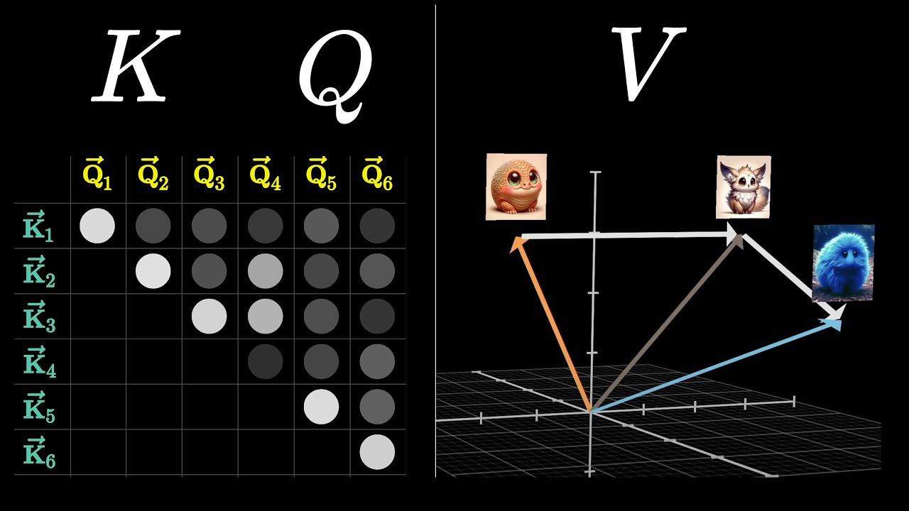
Once softmax is applied across all columns of the dot-product grid, the matrix fills with normalized weights that sum to one down each column. At this stage, the grid functions as an attention pattern: each column specifies how relevant every prior token on the vertical axis is to the token positioned at the top of that column.

```mermaid flowchart TD accTitle: Attention Pattern Calculation accDescr: Pipeline showing Query and Key vectors combined into an attention grid, scaled, masked, and normalized via softmax.

subgraph Inputs["1. Vector Inputs"] Q["Query Vectors (Q)"] K["Key Vectors (K)"] end

subgraph Scoring["2. Raw Dot Products"] Dot["Grid of Dot Products<br/>Q · K^T"] Scale["Scale by 1 / sqrt(d_k)"] end

subgraph PostProcessing["3. Normalization"] Mask["Mask Upper Triangle<br/>(set future to -inf)"] Softmax["Softmax (Column-by-Column)"] Pattern["Attention Pattern Grid"] end

Q --> Dot K --> Dot Dot --> Scale Scale --> Mask Mask --> Softmax Softmax --> Pattern ```

In the original transformer literature (*Attention Is All You Need*), this entire sequence of operations is condensed into a single algebraic expression:

$$\text{Attention}(Q, K, V) = \text{softmax}\left(\frac{Q K^T}{\sqrt{d_k}}\right)V$$

The symbols $Q$ and $K$ denote the full matrices of query and key vectors obtained by multiplying input embeddings by the respective query and key weight matrices. The numerator $Q K^T$ generates the full grid of pairwise dot products. For numerical stability during gradient calculations, each dot product is divided by $\sqrt{d_k}$, where $d_k$ represents the dimension of the smaller key-query space. Finally, the softmax operator is evaluated on a column-by-column basis so that each column forms a valid probability distribution.

---

[11:08](https://www.youtube.com/watch?v=eMlx5fFNoYc&t=668s) Masking and the Context Size Bottleneck

During training, large language models do not merely predict the final token of a training sequence; they simultaneously predict the target next word following every initial subsequence in the passage. For an input passage like *"the fluffy blue creature"*, the model evaluates predictions after *"the"*, after *"the fluffy"*, and after *"the fluffy blue"* all in a single forward pass. Grant Sanderson emphasizes why this architecture is foundational to modern language modeling: “This is really nice, because it means what would otherwise be a single training example effectively acts as many.”

This training efficiency creates an immediate requirement: later tokens must never be permitted to broadcast information backward to earlier tokens, because reading ahead would allow the model to cheat on its next-token prediction task. To prevent future tokens from influencing past ones, the upper-right entries of the attention grid must evaluate strictly to zero. Simply overriding those slots with zeros after the fact fails because the remaining values in the column would no longer sum to one. To resolve this:

- Every entry corresponding to a future token is set to $-\infty$ prior to normalization. - Applying $\text{softmax}(z_i) = \frac{e^{z_i}}{\sum e^{z_j}}$ converts every $-\infty$ into $e^{-\infty} = 0$. - The remaining, valid historical entries renormalize cleanly to sum to $1.0$.

This technique is known as **masking**. While masking is strictly mandatory during training to enforce causal order, GPT-style models maintain this causal mask during inference as well. Because the resulting attention grid compares every token against every other token, its dimensions are $N \times N$, scaling quadratically ($O(N^2)$) with the context window length $N$. Consequently, context length constitutes one of the steepest computational bottlenecks in modern deep learning architectures.

---

[13:10](https://www.youtube.com/watch?v=eMlx5fFNoYc&t=790s) Value Vectors and Updating Embeddings

Once the attention pattern establishes how tokens relate to one another, the architecture needs an actual mechanism to transfer semantic content between them. If the model determines that *"fluffy"* is highly relevant to *"creature"*, the embedding for *"creature"* must shift within the 12,288-dimensional embedding space to encode the specific concept of a fluffy creature.

```mermaid flowchart LR accTitle: Value Vector Weighting and Residual Addition accDescr: Sequence showing token embeddings transformed by the Value matrix, weighted by attention weights, and added back into the target embedding.

subgraph Transform["1. Value Projection"] E["Token Embeddings<br/>('Fluffy', 'Blue')"] Wv["Value Matrix (W_V)"] V["Value Vectors (V)"] end

subgraph Accumulate["2. Weighted Sum"] W["Attention Weights (Col)"] Delta["Delta e (Change Vector)"] end

subgraph Residual["3. Embedding Update"] Orig["Context-Free Embedding<br/>('Creature')"] Out["Refined Embedding<br/>('Fluffy Blue Creature')"] end

E --> Wv --> V V --> Delta W --> Delta Delta --> Out Orig --> Out ```

To achieve this, the model employs a third learned matrix: the **value matrix** ($W_V$). When multiplied by the embedding of an antecedent token (such as *"fluffy"*), the value matrix produces a **value vector**. Grant Sanderson characterizes the conceptual purpose of this operation: “When you multiply this value matrix by the embedding of a word, you might think of it as saying, if this word is relevant to adjusting the meaning of something else, what exactly should be added to the embedding of that something else in order to reflect this?”

These value vectors reside in the identical high-dimensional space as the original embeddings. The updating sequence proceeds systematically across every column: 1. The antecedent tokens produce individual value vectors via the value transformation. 2. In the target token's column (e.g., *"creature"*), each antecedent's value vector is scaled by the corresponding attention weight calculated earlier. High-attention tokens like *"fluffy"* and *"blue"* retain large proportions, while irrelevant tokens receive near-zero weights. 3. The scaled vectors are summed together into a single composite update vector, denoted as $\Delta e$. 4. This displacement $\Delta e$ is added directly to the original context-free embedding of the word.

Executing this weighted summation across all columns yields a completely updated sequence of context-rich vectors across the entire attention block.

---

[15:44](https://www.youtube.com/watch?v=eMlx5fFNoYc&t=944s) Counting Parameters and Low-Rank Value Factorization

A single self-attention head is parameterized by its key, query, and value transformations. Tracking parameter counts using GPT-3's concrete architecture reveals an asymmetry that motivates low-rank factorization:

| Transformation Matrix | Input Dimension | Output Dimension | Total Parameters | |:--- |:--- |:--- |:--- | | **Query Matrix ($W_Q$)** | $12,288$ (Embedding dim) | $128$ (Head dim) | $\approx 1.57 \times 10^6$ | | **Key Matrix ($W_K$)** | $12,288$ (Embedding dim) | $128$ (Head dim) | $\approx 1.57 \times 10^6$ | | **Value Matrix (Naive Square)** | $12,288$ (Embedding dim) | $12,288$ (Embedding dim) | $\approx 150.99 \times 10^6$ | | **Value-Down Matrix ($W_{V,\text{down}}$)** | $12,288$ (Embedding dim) | $128$ (Head dim) | $\approx 1.57 \times 10^6$ | | **Value-Up Matrix ($W_{V,\text{up}}$)** | $128$ (Head dim) | $12,288$ (Embedding dim) | $\approx 1.57 \times 10^6$ |

If the value map were implemented directly as a full square matrix mapping the 12,288-dimensional space back onto itself, that single transformation would demand over 150 million parameters—vastly outnumbering the key and query maps. As Sanderson notes, “You could devote orders of magnitude more parameters to the value map than to the key and query. But in practice, it is much more efficient if instead you make it so that the number of parameters devoted to this value map is the same as the number devoted to the key and the query.”

In practice, the value operation is factored into the product of two rectangular low-rank matrices: - **Value-Down Matrix:** Maps the 12,288-dimensional token embedding down into a compact 128-dimensional latent channel. - **Value-Up Matrix:** Projects that 128-dimensional vector back up into the full 12,288-dimensional embedding space to form the additive displacement $\Delta e$.

In linear algebra terms, this factorization constrains the value transformation to have a mathematical rank of at most 128. By structuring the value operator as two matrices of size $128 \times 12,288$, each of the four components ($W_Q, W_K, W_{V,\text{down}}, W_{V,\text{up}}$) contains approximately 1.57 million parameters, totaling roughly 6.3 million parameters for one complete attention head.

---

[18:21](https://www.youtube.com/watch?v=eMlx5fFNoYc&t=1101s) Cross-Attention vs. Self-Attention

The attention mechanism described up to this point is specifically **self-attention**, because queries, keys, and values are all drawn from the same input sequence. This contrasts with **cross-attention**, an architecture used when models bridge two distinct streams of data, such as machine translation (pairing a source sentence in one language with a target sentence in another) or speech recognition (pairing raw audio features with output text).

In a cross-attention setup: - The keys and values typically derive from the source modality (for example, the original English text). - The queries derive from the target sequence being generated (for example, the ongoing German translation). - The resulting attention pattern aligns tokens across languages, determining which source terms inform the next translated word. - Unlike autoregressive self-attention, cross-attention generally omits causal masking, because the complete source sentence is already fully available to every query step.

Returning to self-attention in generative language models, a single attention head captures only one specific semantic relationship at a time—such as an adjective modifying a subsequent noun. Natural language exhibits countless overlapping semantic dynamics: preceding phrases like *"they crashed the"* fundamentally alter physical assumptions about a subsequent word like *"car"*. Modeling the full richness of human language requires running many attention heads simultaneously in parallel.

[19:49](https://www.youtube.com/watch?v=eMlx5fFNoYc&t=1189s) Multi-Headed Attention

The real strength of the attention mechanism emerges when the network must disentangle complex, ambiguous contextual clues. If the word "wizard" appears anywhere in the same passage as "Harry," the embedding should naturally shift toward Harry Potter. Conversely, if words such as "Queen," "Sussex," and "William" appear in that passage, the embedding for "Harry" ought to be updated to represent Prince Harry. Each distinct type of contextual update requires its own specialized set of key and query matrices to capture the relevant attention pattern, paired with a dedicated value map that decides exactly what semantic shift should be added to the embedding. While real-world trained parameters are far harder to interpret than these clean conceptual vignettes, their weights are tuned to do whatever is necessary to minimize next-token prediction loss.

To execute all these contextual adjustments at once, transformers use multi-headed attention. Rather than relying on a single attention head, a full transformer attention block runs dozens of these operations in parallel, with each head maintaining its own distinct key, query, and value maps. In GPT-3, for instance, each block contains 96 attention heads operating simultaneously.

```mermaid flowchart TD accTitle: Multi-Headed Attention Architecture accDescr: Diagram showing how multiple attention heads compute proposed updates from token embeddings in parallel and sum them into a refined embedding.

subgraph Inputs["Input Sequence"] X["Original Token Embeddings"] end

subgraph Heads["Parallel Attention Heads"] H1["Head 1: Q1, K1, V1<br/>Attention Pattern 1"] H2["Head 2: Q2, K2, V2<br/>Attention Pattern 2"] HDots["..."] H96["Head 96: Q96, K96, V96<br/>Attention Pattern 96"] end

subgraph Aggregation["Update Combination"] Sum["Sum of Proposed Updates<br/>(Head 1 +... + Head 96)"] Out["Refined Token Embeddings"] end

X --> H1 X --> H2 X --> HDots X --> H96 H1 --> Sum H2 --> Sum HDots --> Sum H96 --> Sum X --> Out Sum --> Out ```

Grant Sanderson acknowledges how bewildering this scaling can feel when trying to picture it all at once, noting that “considering that each one is already a bit confusing, it's certainly a lot to hold in your head.” He emphasizes that the underlying objective remains straightforward: “The overall idea is that by running many distinct heads in parallel, you're giving the model the capacity to learn many distinct ways that context changes meaning.”

- GPT-3 utilizes 96 parallel attention heads within each attention block. - Each head computes its own independent attention pattern using its dedicated key and query matrices. - Each head produces a sequence of value vectors and outputs a proposed update vector for every token position. - The proposed changes from all 96 heads are summed together and added directly back to the original token embedding. - With 96 heads per block (each using four matrices across keys, queries, and factored values), each multi-headed attention block accounts for approximately 600 million parameters.

---

[22:16](https://www.youtube.com/watch?v=eMlx5fFNoYc&t=1336s) The Output Matrix Formulation

When looking at literature and open-source implementations, there is a minor mechanical difference from the conceptual view of two distinct value matrices per head. In earlier conceptual breakdowns, the value transformation was explained as two separate operators: a "value down" projection into a lower-dimensional space, followed by a "value up" projection back into the full embedding space. Although one could validly implement each attention head with its own self-contained pair of up and down matrices, practical models do not structure them that way.

Instead, machine learning papers and production code combine all the "value up" matrices across every single head into one unified projection known as the output matrix, which is tied to the entire multi-headed attention block. When researchers and practitioners casually talk about the "value matrix" of an individual attention head, they are almost always referring solely to the initial projection down into the low-rank subspace. Sanderson highlights this implementation detail so that viewers encountering official Transformer codebases will not get tripped up by the differing notation.

---

[23:19](https://www.youtube.com/watch?v=eMlx5fFNoYc&t=1399s) Stacking Layers and Parameter Totals

A transformer does not rely on a single multi-headed attention layer to understand language. Instead, data passes alternately through attention blocks and multi-layer perceptrons (MLPs), repeated across dozens of sequential layers. This deep recurrence allows embeddings to become iteratively richer: once a word absorbs an initial layer of local context, subsequent attention blocks let that newly contextualized representation interact with surrounding tokens that have also been enriched.

As representations travel deeper through the network, the embeddings transcend surface-level syntax and immediate descriptors. They begin to encode abstract properties such as tone, poetic style, literary genre, and underlying scientific concepts.

```mermaid flowchart LR accTitle: Deep Transformer Layer Flow accDescr: Flowchart illustrating the sequential processing of embeddings through alternating attention blocks and multilayer perceptrons across deep layers.

subgraph Layer1["Layer 1"] Attn1["Multi-Headed Attention"] --> MLP1["Multi-Layer Perceptron"] end

subgraph LayerN["Deeper Layers"] AttnN["Multi-Headed Attention"] --> MLPN["Multi-Layer Perceptron"] end

Layer1 -->|"Contextualized Embeddings"| LayerN LayerN --> Abstract["High-Level Representations<br/>(Tone, Sentiment, Knowledge)"] ```

Summing up the total footprint across GPT-3's architecture reveals a surprising distribution of weights:

- GPT-3 contains 96 distinct layers, meaning the ~600 million parameters in a single attention block are repeated 96 times. - This results in just under 58 billion total parameters dedicated exclusively to key, query, and value attention mechanisms. - While 58 billion is massive, it represents only roughly one-third of GPT-3’s 175 billion total parameters. - Sanderson points out that “even though attention gets all of the attention, the majority of parameters come from the blocks sitting in between these steps.”

---

[24:54](https://www.youtube.com/watch?v=eMlx5fFNoYc&t=1494s) Parallelism and Recommended Resources

The true secret weapon behind the dominance of transformers is not merely their expressive modeling capabilities, but their hardware efficiency. Attention can be expressed cleanly as large matrix multiplications, making it exceptionally well suited for massive parallelization on modern GPUs. Sanderson emphasizes that “a big part of the story for the success of the attention mechanism is not so much any specific kind of behaviour that it enables, but the fact that it's extremely parallelizable, meaning that you can run a huge number of computations in a short time using GPUs.” Because the primary empirical lesson of modern deep learning has been that raw scale yields dramatic qualitative leaps in capability, architectures that maximize parallel computing throughput inherently outpace their rivals.

Sanderson concludes with pointers to foundational resources for those seeking to build or understand transformers from first principles: - The work of Andrej Karpathy (including building GPT models from scratch) and Chris Olah (interpretability and transformer circuits), describing their output as "pure gold." - Educational videos by Vivek from the channel *vcubingx*, exploring the historical motivations that lead to reinventing attention. - Britt Cruise's historical retrospective on large language models on the channel *The Art of the Problem*.

## Notable quotes > [24:54](https://www.youtube.com/watch?v=eMlx5fFNoYc&t=1494s) A big part of the story for the success of the attention mechanism is not so much any specific kind of behaviour that it enables, but the fact that it's extremely parallelizable. — Grant Sanderson

> [19:49](https://www.youtube.com/watch?v=eMlx5fFNoYc&t=1189s) The overall idea is that by running many distinct heads in parallel, you're giving the model the capacity to learn many distinct ways that context changes meaning. — Grant Sanderson

> [00:00](https://www.youtube.com/watch?v=eMlx5fFNoYc&t=0s) The aim of a transformer is to progressively adjust these embeddings so that they don't merely encode an individual word, but instead they bake in some much, much richer contextual meaning. — Grant Sanderson

## Mentioned 3Blue1Brown, Grant Sanderson, Attention Is All You Need, GPT-3, Andrej Karpathy, Chris Olah, Anthropic, Vivek, vcubingx, Britt Cruise, The Art of the Problem, Vincent Rubinetti, Manim

## Video description Demystifying attention, the key mechanism inside transformers and LLMs. Instead of sponsored ad reads, these lessons are funded directly by viewers: https://3b1b.co/support Special thanks to these supporters: https://www.3blue1brown.com/lessons/attention#thanks An equally valuable form of support is to simply share the videos.

Demystifying self-attention, multiple heads, and cross-attention. Instead of sponsored ad reads, these lessons are funded directly by viewers: https://3b1b.co/support

The first pass for the translated subtitles here is machine-generated and, therefore, notably imperfect. To contribute edits or fixes, visit https://www.criblate.com

Звуковая дорожка на русском языке: Влад Бурмистров.

------------------

Here are a few other relevant resources

Build a GPT from scratch, by Andrej Karpathy https://youtu.be/kCc8FmEb1nY

If you want a conceptual understanding of language models from the ground up, @vcubingx just started a short series of videos on the topic: https://youtu.be/1il-s4mgNdI?si=XaVxj6bsdy3VkgEX

If you're interested in the herculean task of interpreting what these large networks might actually be doing, the Transformer Circuits posts by Anthropic are great. In particular, it was only after reading one of these that I started thinking of the combination of the value and output matrices as being a combined low-rank map from the embedding space to itself, which, at least in my mind, made things much clearer than other sources. https://transformer-circuits.pub/2021/framework/index.html

Site with exercises related to ML programming and GPTs https://www.gptandchill.ai/codingproblems

History of language models by Brit Cruise,  @ArtOfTheProblem  https://youtu.be/OFS90-FX6pg

An early paper on how directions in embedding spaces have meaning: https://arxiv.org/pdf/1301.3781.pdf

------------------

Timestamps: 0:00 - Recap on embeddings 1:39 - Motivating examples 4:29 - The attention pattern 11:08 - Masking 12:42 - Context size 13:10 - Values 15:44 - Counting parameters 18:21 - Cross-attention 19:19 - Multiple heads 22:16 - The output matrix 23:19 - Going deeper 24:54 - Ending

------------------

These animations are largely made using a custom Python library, manim. See the FAQ comments here: https://3b1b.co/faq#manim https://github.com/3b1b/manim https://github.com/ManimCommunity/manim/

All code for specific videos is visible here: https://github.com/3b1b/videos/

The music is by Vincent Rubinetti. https://www.vincentrubinetti.com https://vincerubinetti.bandcamp.com/album/the-music-of-3blue1brown https://open.spotify.com/album/1dVyjwS8FBqXhRunaG5W5u

------------------

3blue1brown is a channel about animating math, in all senses of the word animate. If you're reading the bottom of a video description, I'm guessing you're more interested than the average viewer in lessons here. It would mean a lot to me if you chose to stay up to date on new ones, either by subscribing here on YouTube or otherwise following on whichever platform below you check most regularly.

Mailing list: https://3blue1brown.substack.com Twitter: https://twitter.com/3blue1brown Instagram: https://www.instagram.com/3blue1brown Reddit: https://www.reddit.com/r/3blue1brown Facebook: https://www.facebook.com/3blue1brown Patreon: https://patreon.com/3blue1brown Website: https://www.3blue1brown.com

[Source](https://www.youtube.com/watch?v=eMlx5fFNoYc)

中文简报

Transformer 注意力机制逐步解析 | 深度学习第 6 章 该视频详细剖析了 Transformer 如何利用注意力机制,将静态、孤立的 token 嵌入转换为预测下一个词所需的丰富语境感知表征。Sanderson 解释了查询(Query)、键(Key)、点积相关性得分和掩码的线性代数原理,展示了按列进行的 Softmax 如何生成控制信息传递的注意力模式网格。他详细阐述了值向量(Value)如何通过加权并经由低秩分解累加回 token 嵌入中,这一过程结合了分布在数十个并行头和深层网络中的多头注意力机制。最后,他将这些理论矩阵运算与 GPT-3 等现实架构联系起来,强调现代 Transformer 的卓越性能不仅取决于概念上的表达能力,同样高度依赖其契合 GPU 的可并行性。 自注意力机制通过将输入投影到学习得到的查询、键和值空间来计算有向向量更新,从而将静态 token 嵌入转换为依赖上下文的表征。 (0:00) 为防止在自回归训练和推理过程中未来 token 泄漏到过去的预测中,注意力得分在应用按列 Softmax 之前会被负无穷大掩码。 (11:08) 为避免像 GPT-3 这样的架构中每个注意力头产生多达 1.5 亿参数的完整全方阵映射,值变换被分解为通过 128 维瓶颈层的低秩降维和升维投影。 (15:44) 尽管注意力机制在概念上备受瞩目,但在 GPT-3 的 1750 亿总参数中,它占用的参数不足 580 亿,大部分参数实际上存在于中间的前馈 MLP 层中。 (23:19)

Reading summary

Grant Sanderson of 3Blue1Brown explains that the transformer attention mechanism iteratively refines static token embeddings into rich, context-aware representations by computing directional update vectors across sequences. While attention is conceptually framed as an interpretive linguistic tool, its practical dominance stems primarily from its high degree of parallelizability across matrix multiplications on modern GPU hardware. Contextualizing Static Embeddings Through Vector Deltas (0:00) Language models begin by assigning tokens static vectors in a high-dimensional embedding space where geometric directions denote semantic properties. Because lookup tables assign identical vectors to polysemic terms regardless of meaning—such as 'mole' across biology, chemistry, or medicine—a network must compute displacement vectors to push base tokens toward correct contextual interpretations. In autoregressive next-token prediction, this dynamic culminates in a bottleneck where the sequence's final token vector must absorb all preceding clues across the context window. Alignment Scores, Column Softmax, and Causal Masking (4:29) To identify which antecedents should update a given token, learned weight matrices project embeddings into lower-dimensional key and query spaces. Pairwise dot products assess semantic alignment, generating raw attention scores ranging from negative to positive infinity. Evaluating these scores through a column-by-column softmax function normalizes each column into a valid probability distribution that dictates contextual relevance. Causal Masking and Context Window Scaling (11:08) Training models to predict the target word after every initial subsequence requires causal masking, where future matrix entries are assigned values of negative infinity prior to softmax. This ensures earlier tokens cannot attend forward and cheat during prediction, converting future entries cleanly to zero while historical weights renormalize to one. Because the resulting attention grid compares all tokens against one another, memory and computation scale quadratically with context length, creating a significant architecture bottleneck. Value Transformation and Low-Rank Factorization (13:10) Once attention weights are established, embeddings are updated using value matrices that define what vector displacement should be transferred from an antecedent token. To avoid dedicating excessive parameters to a full square value matrix—which would require roughly 150 million weights in a 12,288-dimensional embedding space—models factor the operation into low-rank down and up projections constrained to a head dimension such as 128. Weighted value vectors are summed into a composite change vector and added back directly to the original token embedding. Multi-Headed Scaling and Hardware Efficiency (19:49) To capture diverse, overlapping contextual dynamics simultaneously, models deploy multi-headed attention blocks. In GPT-3, 96 parallel heads generate distinct proposed updates per block, combining into an additive update representing roughly 600 million parameters per layer. Across GPT-3's 96 layers, attention mechanisms account for approximately 58 billion parameters—roughly one-third of the total 175 billion parameter budget, with the remainder housed in alternating feedforward blocks. Sanderson highlights that the ultimate success of the attention mechanism relies less on any singular qualitative behavior than on its hardware efficiency. Expressed cleanly as large matrix operations, attention maximizes GPU throughput, enabling the sheer scale that drives empirical leaps in model capability.

精炼阅读摘要

Grant Sanderson在讲解中指出,Transformer的核心机制是通过注意力模块将孤立、静态的词嵌入逐步调整为蕴含丰富上下文的高维向量,从而实现精准的下一个词预测。其工程成功不仅源于丰富的语义表征能力,更得益于能够高度适配现代GPU并行计算的矩阵乘法结构。 词嵌入的局限与上下文动态调整 (0:00) 在Transformer架构中,输入的文本首先被切分为Token,并在高维嵌入空间中初始化为向量。该空间的基本几何特性体现为特定几何方向对应具体语义变化,例如对阳性名词施加位移向量可使其指向对应的阴性名词。然而,静态查找表赋予同一个词相同的初始向量,无法应对一词多义现象。例如在生物学的“鼩鼹”(shrew mole)、化学单位“摩尔”(mole)以及医学“切片检查痣”(biopsy of the mole)中,“mole”一词的初始嵌入完全一致,必须依赖注意力模块计算向量差值,将其推向正确的语义方向。类似地,“tower”在加入“Eiffel”或“miniature”等修饰语后,也需要动态调整其尺寸与地理关联。此外,自回归模型对下一个词的预测完全依赖序列末尾的最后一个向量,该向量必须借助注意力块吸收整个上下文窗口内的所有关键信息,才能完成前瞻预测。 查询、键匹配与因果掩码归一化 (4:29) 注意力机制通过查询(Query)和键(Key)的交互量化词语间的相关度。以包含位置编码的嵌入向量e为输入,模型通过可学习的权重矩阵$W_Q$和$W_K$分别将其投影到较低维度的空间(例如128维),生成查询向量q与键向量k。查询向量提出语义检索问题(例如名词寻找先前的修饰形容词),而键向量广播自身特征属性。二者通过点积($q \cdot k$)计算相关性得分,得分越高代表对齐程度越强。随后,原始点积除以标量$\sqrt{d_k}$以保障梯度稳定,并在列方向上应用Softmax函数,将数值转化为和为1的概率分布权重,形成标准的注意力模式。在自回归语言模型中,为了防止模型在训练预测下一个词时“偷看”后续内容,未来的注意力得分在归一化前会被强制设为$-\infty$(经Softmax后为0),这一因果掩码技术使得单次前向传播能够同时评估序列中每个子序列的预测。但该机制形成的$N \times N$网格也导致计算量与上下文长度呈$O(N^2)$二次方增长,成为模型扩展的主要算力瓶颈。 值向量变换、低秩分解与参数控制 (13:10) 当注意力权重确定后,模型需要具体机制将语义内容注入目标词。该过程通过值权重矩阵$W_V$实现:前序词的嵌入经$W_V$映射为值向量(Value),按注意力权重加权求和,生成综合更新向量$\Delta e$,最后残差叠加回目标词的原始嵌入中。若将值映射直接实现为12,288维的全尺寸方阵,单头参数量将超1.5亿;为平衡参数量,工程实践中将值矩阵因式分解为两个低秩矩阵:首先通过“下投影矩阵”($W_{V,\text{down}}$)降至128维低秩空间,再通过“上投影矩阵”($W_{V,\text{up}}$)投回12,288维空间,将变换的数学秩限制在128以内。如此设计使得$W_Q$、$W_K$、$W_{V,\text{down}}$与$W_{V,\text{up}}$各自拥有约157万参数,单个注意力头参数总量约为630万。在实际工程与开源代码实现中,各头的上投影操作通常被整合为针对整个多头模块的单一统一输出矩阵。 多头并行机制与深度堆叠架构 (19:49) 单个自注意力头仅能捕捉一种特定的语义关联模式,而自然语言包含大量交叠的上下文线索(例如区分“哈利”是指哈利·波特还是哈利王子)。Transformer通过多头注意力机制并行运行多个具有独立权重矩阵的注意力头,使模型具备同时学习多维度语义调整的能力。以GPT-3为例,每个注意力块包含96个并行头,单块参数量约达6亿,各头计算出的更新向量直接累加后加回原始输入。网络通过交替堆叠多头注意力块与多层感知机(MLP)达96层,使嵌入向量在逐层传递中由表层语法逐渐演进为对语调、文学体裁及抽象科学概念的高阶表征。在GPT-3的1750亿总参数中,注意力机制占用了约580亿,而感知机层占据了剩余的三分之二多数参数。除同序列交互的自注意力外,跨语言翻译或语音识别等跨模态任务则采用不设因果掩码的交叉注意力架构,将生成序列的查询与源序列的键和值进行对齐。 Sanderson强调,Transformer之所以能在当代人工智能中占据主导地位,不仅取决于其丰富的语义表达能力,更核心的优势在于其计算流程高度依赖矩阵乘法,与GPU的极速并行架构天然契合,从而使现代深度学习能够通过持续扩大算力与参数规模获得质的性能飞跃。

Detailed notes — zh

## Background 本内容由知名数学科普频道 3Blue1Brown(Grant Sanderson)于 2024 年 4 月 7 日发布在 YouTube 平台上。该视频为深度学习系列教程的第六章,主要围绕大语言模型与 Transformer 的核心算法展开,旨在循序渐进地拆解自注意力机制、掩码、多头注意力及交叉注意力等关键概念。 ## TL;DR 视频深入剖析了 Transformer 如何通过注意力机制打破静态词嵌入的局限,动态融入丰富的上下文语义。Grant Sanderson 借助形容词修饰名词的直观案例,逐步推导了 Query、Key 与 Value 向量的矩阵运算、点积打分及 Softmax 掩码归一化过程,并结合 GPT-3 架构细致核算了单头与多头注意力的参数量与低秩分解。最后,内容阐述了注意力块与 MLP 模块在深层网络中的协同抽象能力,指出注意力机制之所以成为革命性突破,关键在于其架构高度适配 GPU 的并发算力。 ## Atmosphere & style 视频保持了 3Blue1Brown 标志性的从容、严密与优雅风格,通过精湛的可视化几何动画将晦涩抽象的高维线性代数具象呈现。Sanderson 的讲解语调平和沉稳、层层递进,既有对语言学直觉的拟人化引导,又有工程落地细节的理性审视。整场叙事不仅让观众在追踪数据流转的过程中获得豁然开朗的智性愉悦,更深刻体会到现代深度学习算力扩展背后的数学美感。 ## Bulletin - [04:29](https://www.youtube.com/watch?v=eMlx5fFNoYc&t=269s) Transformer 通过 Query 与 Key 矩阵降维投影后计算点积与 Softmax 分数,将多义词与上下文特征动态叠加回初始嵌入向量,打破了静态查表无上下文的语义局限。 - [11:08](https://www.youtube.com/watch?v=eMlx5fFNoYc&t=668s) 自注意力机制采用掩码技术在 Softmax 前将未来位置注意力得分赋为负无穷,既支持了训练阶段多位置并行预测,又杜绝了后文信息泄露。 - [15:44](https://www.youtube.com/watch?v=eMlx5fFNoYc&t=944s) 工程上通过低秩分解将 Value 映射拆分为 Value-Down 与 Value-Up(输出矩阵),使 GPT-3 单个注意力头的参数量控制在约 6.3M,整体单块参数约为 6 亿。 - [23:19](https://www.youtube.com/watch?v=eMlx5fFNoYc&t=1399s) 在 GPT-3 的 1750 亿总参数中,注意力机制占近 580 亿(约三分之一),其余绝大部分权重分布于各层穿插的 MLP 等前馈网络中。 ## Key takeaways - [00:00](https://www.youtube.com/watch?v=eMlx5fFNoYc&t=0s) 初始 Token Embedding 只是无上下文的静态查表,Transformer 的核心任务是利用注意力机制向向量注入特定语义偏移量。 - [01:40](https://www.youtube.com/watch?v=eMlx5fFNoYc&t=100s) 在自回归文本生成中,预测下一个 Token 的全部推理信息最终必须浓缩汇聚进序列的最后一个向量。 - [04:29](https://www.youtube.com/watch?v=eMlx5fFNoYc&t=269s) Query 向量编码当前词需要寻找的上下文需求,Key 向量编码自身可供检索的特征,二者点积衡量相关性强度。 - [10:00](https://www.youtube.com/watch?v=eMlx5fFNoYc&t=600s) 点积计算需除以维度平方根以维持数值稳定性,并通过列方向 Softmax 转换为总和为 1 的归一化概率分布。 - [11:08](https://www.youtube.com/watch?v=eMlx5fFNoYc&t=668s) 因果掩码通过在 Softmax 前将上三角后文得分置为负无穷,使单个训练样本能同时高效并行预测各前缀子序列的下一个词。 - [12:42](https://www.youtube.com/watch?v=eMlx5fFNoYc&t=762s) 注意力模式网格尺寸随序列长度呈二次方(N^2)增长,这是限制大语言模型上下文窗口扩展的核心计算瓶颈。 - [13:10](https://www.youtube.com/watch?v=eMlx5fFNoYc&t=790s) Value 矩阵决定了在相关度加权后具体向目标嵌入注入什么语义信息,并通过残差连接将增量叠加回原向量。 - [15:44](https://www.youtube.com/watch?v=eMlx5fFNoYc&t=944s) 若直接采用全尺寸方阵做 Value 变换会导致参数爆炸,通过低秩分解为两个较小矩阵可大幅压缩显存与参数规模。 - [18:21](https://www.youtube.com/watch?v=eMlx5fFNoYc&t=1101s) 与自注意力不同,交叉注意力分别从源文本与目标文本提取 Key 与 Query,且通常无需使用因果掩码机制。 - [19:49](https://www.youtube.com/watch?v=eMlx5fFNoYc&t=1189s) 多头注意力机制并行运行多套独立的 Q、K、V 映射,赋予模型同时捕捉语法、常识和语境改变语义的多种不同模式的能力。 - [22:16](https://www.youtube.com/watch?v=eMlx5fFNoYc&t=1336s) 学术文献与工程实现中通常将各头的升维映射拼接为统一的输出矩阵,并将降维矩阵单独称为该头的 Value 矩阵。 - [23:19](https://www.youtube.com/watch?v=eMlx5fFNoYc&t=1399s) 虽然注意力机制广受关注,但 GPT-3 模型中约三分之二的参数实际上集中在注意力块之间交替穿插的 MLP 模块中。 - [24:54](https://www.youtube.com/watch?v=eMlx5fFNoYc&t=1494s) 注意力机制主导现代深度学习的关键优势在于其极高的数据并行性,能够最大化利用 GPU 算力并在参数扩展中实现性能质变。 ## Detailed walkthrough ### [00:00](https://www.youtube.com/watch?v=eMlx5fFNoYc&t=0s) 回顾 Embedding 与上下文信息的缺失 在深入 Transformer 的内部构造之前,有必要先明确语言模型的基本设定:模型的目标是接收一段文本输入,并预测紧接着出现的下一个词。输入的文本会被拆解为被称为 Token(标记)的微小片段。虽然在真实的现代大语言模型中 Token 通常是词或词的一部分,但为了便于直观理解,可以暂且将每个 Token 简化为单个独立的单词。 进入模型的第一步,是将每个 Token 映射为一个高维空间中的向量,即词嵌入(Embedding)。这一机制的核心直觉在于:**高维嵌入空间中的特定几何方向对应着某种抽象的语义**。正如上一章节所展示的例子,沿着特定方向位移可以实现从男性名词到对应女性名词的平移转换。然而,仅靠初始的 Token Embedding 存在严重的语义局限性——它本质上是一个静态的查表操作(Lookup Table),完全不包含任何上下文信息。Transformer 的根本目标,就是通过层层计算不断修正并微调这些向量,使得它们不再仅仅代表孤立的单词,而是融合极度丰富的上下文语境。 “The aim of a transformer is to progressively adjust these embeddings so that they don't merely encode an individual word, but instead they bake in some much, much richer contextual meaning.”(Grant Sanderson 强调道:“Transformer 的目标是逐步调整这些嵌入向量,使它们不再仅仅编码单个词,而是融入更加丰富的上下文含义。”) ```mermaid flowchart LR accTitle: Token Embedding Lookup to Contextual Adjustment accDescr: Diagram showing how static token embeddings are mapped from tokens and then adjusted into contextualized embeddings. subgraph InputStage["输入与查表"] T["输入文本 Tokens"] --> L["静态查表 Embedding Table"] L --> E["初始 Embedding e<br/>(无上下文/仅自身语义)"] end subgraph ModelProcessing["Transformer 核心演进"] E --> A["Attention 机制与多层网络"] A --> C["富含上下文的向量<br/>(融入深层语境)"] end ``` --- ### [01:40](https://www.youtube.com/watch?v=eMlx5fFNoYc&t=100s) 为什么需要注意力机制:多义词与长程信息流动的现实案例 许多人在初次接触 Attention(注意力机制)时常感到晦涩困惑,因此在铺开繁杂的矩阵乘法之前,先考察几个它试图解决的典型语言场景至关重要。以英语中的多义词“mole”为例,对比以下三个短语: - “American shrew mole”(美洲鼩鼹,指一种小型哺乳动物) - “one mole of carbon dioxide”(一摩尔二氧化碳,指化学计量单位) - “take a biopsy of the mole”(给这颗痣做活检,指皮肤上的色素痣) 在刚完成词嵌入查表的第一步时,三个短语中对应“mole”的向量是完全一致的。但在高维语义空间中,应当存在数个截然不同的方向分别代表动物、化学单位和皮肤斑痣。一个训练优良的 Attention 模块,任务正是根据“shrew”、“carbon dioxide”或“biopsy”等上下文单词,计算出需要向通用的“mole”向量中注入多大强度的特定方向偏移量,将其精准推向对应的特异性语义方向。 另一个例子是单词“tower”(塔)。孤立来看,它只是一个指向泛化的大型高耸物体的普通向量;如果其前面紧接着出现“Eiffel”(埃菲尔),Attention 机制就应修改该向量,让它偏向巴黎、法国及钢结构等相关概念的方向;而如果在前方再加入“miniature”(微型),这个向量又必须被进一步修正,剥离掉原本属于“巨大宏伟”的特征。 更深层次地看,Attention 机制允许模型打破空间距离的限制,在任意 Token 之间搬运与注入信息。在实际生成过程中,预测下一个词的全部运算最终仅仅基于序列中的**最后一个向量**。例如输入一部包含数十万词的长篇侦探小说,文本停在倒数第二句:“因此,凶手就是……”(therefore the murderer was)。最后一个原本仅代表单词“was”的基础向量,必须在穿过层层注意力模块后,如吸星大法般融会贯通整部小说所有的伏笔、线索与逻辑推理,将其全部浓缩进自身数值之中,才能在输出端准确推断出真凶的名字。 - **多义词消歧(Disambiguation)**:初始嵌入处于通用歧义态,依赖注意力模块提取上下文特征向量做线性叠加修正。 - **语义修饰(Attribute Modification)**:形容词或限定词(如 miniature、Eiffel)对名词核心表征的动态调整与重塑。 - **信息汇聚至末位向量(Terminal Bottleneck)**:在自回归生成中,全部跨上下文的推理结果最终都必须编码进最后一个 Token 的向量内部。 --- ### [04:29](https://www.youtube.com/watch?v=eMlx5fFNoYc&t=269s) Query 与 Key:从形容词修饰名词看单头自注意力 为了抽丝剥茧地理清具体的数学计算,可以构建一个极度简化的玩具模型。假设有一句输入文本:“a fluffy blue creature roamed the verdant forest”(一只蓬松的蓝色生物漫步在翠绿的森林中)。在此暂且假定唯一的更新需求是:**让形容词去修正紧随其后的名词**。在底层实现上,这种专项特征提取任务是由单个注意力头(Single Head of Attention)承担的,实际的 Attention Block 则是大量此类注意力头的并行组合。 每个 Token 传入的初始向量记为 $e$。它不仅通过高维坐标表达该词本身的含义,还融入了位置编码(Positional Encoding),使得该向量兼具“词义”与“在上下文中的绝对/相对坐标”。为了在深度学习框架下通过数据自主学习这种关联,全部操作均构建为可学习权重矩阵与向量的乘积运算。 “I'm making up this example of adjectives updating nouns just to illustrate the type of behavior that you could imagine an attention head doing.”(Grant Sanderson 解释说:“我虚构这种由形容词更新名词的例子,仅仅是为了向你们展示注意力头可能执行的某种直观行为。”)在真实神经网络中,数百亿参数联合梯度下降得到的特征往往极其抽象,但借助这种拟人化的语言学假设,可以帮助我们严密追踪数据流的演变: ```mermaid flowchart TD accTitle: Computation of Query and Key Vectors accDescr: Flowchart illustrating the mapping from token embedding through query and key weight matrices down to dot product scoring and softmax. subgraph Inputs["输入 Token 嵌入"] E1["名词嵌入 e (如 creature)"] E2["形容词嵌入 e (如 fluffy / blue)"] end subgraph Projection["降维投影变换"] WQ["Query 权重矩阵 W_q"] WK["Key 权重矩阵 W_k"] E1 -->|乘法| WQ --> Q["Query 向量 q<br/>(提问: 前方有名词修饰我吗?)"] E2 -->|乘法| WK --> K["Key 向量 k<br/>(回答: 我是处于该位置的形容词)"] end subgraph Interaction["相关度匹配"] Q & K --> Dot["点积运算 (q · k)"] Dot --> Grid["原始分数矩阵 (范围: -∞ 到 +∞)"] Grid --> SM["列方向 Softmax 归一化<br/>(转换为概率分布,和为 1)"] end ``` 在这套逻辑中,名词(如“creature”)发出一个询问:“嘿,我的前面有修饰我的形容词吗?”而前面的词(如“fluffy”和“blue”)则回答:“是的,我是形容词,且正好位于修饰你的前置位。” 1. **Query(查询向量 $q$)**:通过让嵌入向量 $e$ 乘以可学习的矩阵 $W_q$ 得到。Query 向量存在于一个维度更低的子空间中(例如 128 维),它编码了当前词“正在寻找什么样的上下文信息”。 2. **Key(键向量 $k$)**:同理,让所有词的嵌入向量 $e$ 乘以另一个同维度的可学习矩阵 $W_k$ 得到 Key 向量。Key 向量编码了当前词“具备什么样的特征可以供给其他词检索”。 3. **点积打分(Dot Product)与相关度度量**:衡量 Key 与 Query 是否匹配的数学手段是计算它们的点积。若两向量夹角极小、方向高度对齐,点积就会输出一个极大的正数;反之,若语义毫无关联(例如冠词“the”与“creature”),点积就会接近零乃至为负数。当“fluffy”与“blue”的 Key 与“creature”的 Query 产生高额点积时,用机器学习的行话来说,就是“fluffy”和“blue”的嵌入向量**被“creature”所关注(attend to)**。 4. **Softmax 归一化**:遍历序列中所有的 Key 与 Query 计算出的点积构成了一个打分网格(Score Grid),其数值理论上涵盖从 $-\infty$ 到 $+\infty$ 的任意实数。由于下一步需要依据相关性强度对信息做加权求和,必须将这些原始打分沿每一列进行 Softmax 变换,把原本杂乱无章的实数转换为区间位于 $[0, 1]$ 之间、且整列总和严格等于 1 的概率权重分布。 ### [10:00](https://www.youtube.com/watch?v=eMlx5fFNoYc&t=600s) 注意力模式与注意力公式 (The Attention Pattern) 在将 Softmax 应用于网格的每一列后,整个网格便填满了归一化后的权重值。此时,可以将每一列理解为分配给左侧词的权重,代表该词与顶部目标词之间的相关程度。这个网格被称为**注意力模式(Attention Pattern)**。在原始的 Transformer 论文中,整个计算过程被极其紧凑地表达为一个数学公式: $$\text{Attention}(Q, K, V) = \text{softmax}\left(\frac{QK^T}{\sqrt{d_k}}\right)V$$ 公式中的变量 $Q$ 和 $K$ 分别代表 Query 和 Key 向量的完整矩阵,也就是将原始嵌入向量分别乘以 Query 权重矩阵和 Key 权重矩阵所得到的小向量。分子中的点积运算 $QK^T$ 是表示所有 Key 与 Query 两两之间点积的简洁形式。公式中包裹在外层的 Softmax 是逐列(column by column)计算的。 这里还存在一个微小的技术细节:为了数值稳定性(Numerical Stability),计算出的点积必须除以 Key 和 Query 向量空间的维度平方根 $\sqrt{d_k}$。至于公式末尾的 $V$ 项,则是接下来用于信息传递的 Value。 ### [11:08](https://www.youtube.com/watch?v=eMlx5fFNoYc&t=668s) 掩码机制与上下文窗口 (Masking & Context Size) 在模型训练过程中,当模型处理某一段文本示例时,所有权重都会根据其为真实下一个词分配的概率高低进行微调。为了大幅提高训练效率,模型并不会每次只预测最后一个词,而是同时预测该序列中每一个初始子序列后面的下一个 Token。例如在短语中,模型在预测最后词的同时,也在同步预测 "the" 后面是什么词、"creature" 后面是什么词。正如 Grant Sanderson 所指出的那样:“This is really nice, because it means what would otherwise be a single training example effectively acts as many.”(这非常巧妙,因为这意味着原本单条的训练样本在实际效果上充当了许多个样本。) 这种并行预测带来了一个硬性约束:**绝不能允许后面的词影响前面的词**,否则后文就会提前“剧透”答案。这意味着在注意力网格中,所有代表“后文 Token 影响前文 Token”的格子都必须被强制归零。 如果直接粗暴地将它们赋值为 0,会导致 Softmax 之后的每一列求和不再等于 1,从而破坏归一化。因此标准的做法是:**在应用 Softmax 之前,将这些位置的注意力得分设为负无穷($-\infty$)**。经过 Softmax 计算后,负无穷会自动转化为严格的 0,同时各列依然保持概率和为 1 的归一化状态。这个过程被称为**掩码(Masking)**。 关于注意力模式,另一个极其关键的特征是其网格尺寸等于上下文长度的平方($N^2$)。这种二次方增长正是上下文尺寸(Context Size)成为大语言模型巨大瓶颈的核心原因,也使得扩展上下文长度变得极具挑战性。 ### [13:10](https://www.youtube.com/watch?v=eMlx5fFNoYc&t=790s) Value 向量与嵌入更新 (Values) 计算出注意力模式仅仅让模型知道了“哪些词与哪些词相关”,接下来必须实际更新嵌入向量,实现信息在词之间的传递。例如,必须让形容词 "Fluffy" 的嵌入能够改变 "Creature" 的嵌入,使其在 12,288 维的嵌入空间中移动到一个更具体编码“毛茸茸生物”的新位置。 最直接的实现方式是引入第三个矩阵——**Value 矩阵**: 1. **生成 Value 向量**:将 Value 矩阵与词的原始嵌入(例如 "Fluffy")相乘,得到一个与嵌入维度相同的 Value 向量。当乘以该矩阵时,它的物理意义可以理解为:“如果这个词与调整其他词的含义相关,那么究竟应该在其他词的嵌入上加上什么,才能体现出这种关联?” 2. **权重加权**:移开先前的 Key 与 Query,将 Value 矩阵与序列中的每一个嵌入相乘得到一系列 Value 向量。在注意力的某一列下(如 "Creature" 列),根据该列计算出的注意力权重,对各个词的 Value 向量进行缩放。与 "Creature" 高度相关的 "Fluffy" 和 "Blue" 会保留较大比例的 Value 向量,而无关的词则被归零或接近归零。 3. **残差相加($\Delta e$)**:将该列所有按权重缩放后的 Value 向量相加,合成一个更新变化量 $\Delta e$。最后将 $\Delta e$ 与 "Creature" 原有的无上下文嵌入相加,生成一个更丰富、融合了“毛茸茸与蓝色”上下文的新嵌入向量。 对序列中所有列同步执行这一加权求和更新,整个注意力块便输出了一组经过上下文洗礼的精细化嵌入向量。 ```mermaid flowchart LR accTitle: Single Head Attention Pipeline accDescr: The computation flow of a single self-attention head including QK matching, masking, softmax weighting, and value addition. subgraph Matching["相似度计算与权重"] E["输入嵌入 Embedding"] --> Q["Query 向量"] E --> K["Key 向量"] Q & K --> Dot["点积除以根号 dk"] Dot --> Mask["掩码 (设为 -inf)"] Mask --> SM["Softmax 归一化"] end subgraph Values["Value 变换与加权累加"] E --> VDown["Value 变换"] VDown --> Val["Value 向量"] SM & Val --> Weighted["依权重缩放并求和"] end Weighted --> Delta["变化量 Delta e"] E --> Add["残差连接相加"] Delta --> Add Add --> Out["更新后的精细嵌入"] ``` ### [15:44](https://www.youtube.com/watch?v=eMlx5fFNoYc&t=944s) 参数量核算与低秩分解 (Counting Parameters) 回顾上述过程,单个注意力头由三个主要的权重矩阵进行参数化:Key、Query 和 Value。以 GPT-3 的真实尺寸进行量化核算: - **Key 矩阵与 Query 矩阵**:输入维度对应嵌入维度的 12,288,输出维度对应较小的 Key-Query 空间 128。每个矩阵包含 $12{,}288 \times 128 \approx 157$ 万个参数。 - **原始 Value 矩阵的困境**:如果 Value 矩阵直接将 12,288 维的嵌入映射到 12,288 维的更新向量,它将是一个 $12{,}288 \times 12{,}288$ 的方阵,单头参数量将飙升至约 1.5 亿。这不仅会消耗比 Key/Query 高出几个数量级的参数,而且在并行运行多头注意力时极度低效。 - **低秩分解(Low-Rank Factorization)**:在工程实践中,Value 变换被分解为两个较小矩阵的乘积: 1. 第一个矩阵(视频中形象地称为 **Value-Down 矩阵**)将 12,288 维的大嵌入压缩到与 Key-Query 空间大小一致的低维空间(128 维),尺寸为 $128 \times 12{,}288$。 2. 第二个矩阵(视频中称为 **Value-Up 矩阵**,通常在论文中表现为最终的输出投影矩阵)从该 128 维空间再映射回 12,288 维的嵌入空间,尺寸为 $12{,}288 \times 128$。 用线性代数的术语来说,这实质上是将整体的 Value 映射限制为一个低秩变换。分解后,四个矩阵(Query、Key、Value-Down、Value-Up)的尺寸完全一致,每个约 157 万参数,合并起来**单个注意力头的参数量约为 630 万**。 - Key 矩阵参数量:$12{,}288 \times 128 \approx 1{,}572{,}864$ - Query 矩阵参数量:$12{,}288 \times 128 \approx 1{,}572{,}864$ - Value-Down 矩阵参数量:$128 \times 12{,}288 \approx 1{,}572{,}864$ - Value-Up 矩阵参数量:$12{,}288 \times 128 \approx 1{,}572{,}864$ - 单注意力头总参数量:$\approx 6{,}291{,}456$(约 6.3M) ### [18:21](https://www.youtube.com/watch?v=eMlx5fFNoYc&t=1101s) 交叉注意力拓展与多头概念引入 (Cross-Attention) 上述机制被称为**自注意力(Self-Attention)**,它处理的是单一序列内部词与词的交互。作为补充,许多模型(如机器翻译模型或语音转录模型)会采用**交叉注意力(Cross-Attention)**: - 交叉注意力处理两组不同的数据源。例如在翻译任务中,Key 来自源语言文本,Query 则来自正在生成的目标语言文本;注意力模式刻画的是源语言词汇与目标语言词汇之间的对应关系。 - 交叉注意力通常不使用因果掩码,因为源语言文本在一开始就是完全可见的,不存在“后文泄露前文答案”的时序因果限制。 回到自注意力机制,单个注意力头演示了形容词如何更新名词,但这仅仅是语境影响词义的冰山一角。例如,在 "They crashed the car" 中,动词短语 "crashed" 会直接改变 "car" 在空间中的形状与结构表征;此外还有无数非语法的常识或逻辑关联。要捕捉自然语言中错综复杂的多维关系,模型绝不能只依赖单一的注意力头,而必须将这一机制并行复制很多次。 ### [19:49](https://www.youtube.com/watch?v=eMlx5fFNoYc&t=1189s) 多头注意力机制的工作原理与参数规模 语境对词义的塑造方式多种多样。如果文章中出现“巫师”(wizard)和“哈利”(Harry),模型会倾向于认为这指的是哈利·波特(Harry Potter);但若文中出现的是“女王”(Queen)、“萨塞克斯”(Sussex)和“威廉”(William),那么“Harry”的词嵌入向量(Embedding)就应当被调整以指向英国王室的哈利王子。为了捕捉不同类型的语境更新,Key 矩阵和 Query 矩阵的参数必须各不相同以形成不同的注意力模式,Value 映射矩阵也需要针对“该往嵌入向量中注入什么信息”进行针对性调整。而在真实训练中,这些权重完全是为了达成模型预测下一个 Token 的目标而自主调整的,人类很难直观解释。 完整的 Transformer 注意力块采用的是多头注意力(Multi-Headed Attention),即在同一个块内并行运行多套独立的 Key、Query 和 Value 映射机制。以 GPT-3 为例,其每一个注意力块内部就包含了 96 个注意力头。这意味着存在 96 组独立的 Key 与 Query 矩阵产生 96 种注意力模式,同时 96 个头各自拥有独立的 Value 矩阵生成对应的 Value 向量序列。对于上下文中的每一个 Token 位置,所有注意力头各自计算出一个“建议更新量”(proposed change),随后将这 96 个建议向量相加并合并到该位置原始的嵌入向量上,从而输出该位置精炼后的全新向量。 3Blue1Brown 总结了设计多头的根本逻辑:“The overall idea is that by running many distinct heads in parallel, you're giving the model the capacity to learn many distinct ways that context changes meaning.”(通过并行运行许多不同的头,你赋予了模型学习‘语境改变语义的诸多不同方式’的能力。) - **并行头数(GPT-3)**:每个注意力块包含 96 个独立的注意力头。 - **单块参数总量**:包含 96 个头各自的四套矩阵映射,单个多头注意力块具有约 6 亿(600M)参数。 ```mermaid flowchart TD accTitle: Multi-Head Attention Data Flow accDescr: A diagram showing input tokens split into 96 attention heads and then summed to produce updated embeddings. subgraph InputStage["输入端"] Tokens["输入 Token 嵌入向量"] end subgraph HeadsStage["多头并行计算 (96 个独立头)"] Head1["头 1: Q, K, V 映射 -> 建议更新量 1"] HeadDots["... 其余注意力头..."] Head96["头 96: Q, K, V 映射 -> 建议更新量 96"] end subgraph CombineStage["汇聚输出"] SumNode["累加 96 个头的建议更新量"] OutputTokens["输出:精炼后的全新词嵌入向量"] end Tokens --> Head1 Tokens --> HeadDots Tokens --> Head96 Head1 --> SumNode HeadDots --> SumNode Head96 --> SumNode Tokens -->|"残差连接相加"| OutputTokens SumNode --> OutputTokens ``` ### [22:16](https://www.youtube.com/watch?v=eMlx5fFNoYc&t=1336s) 输出矩阵的实际工程实现与文献差异 在具体的工程实现和学术论文中,Value 映射的表述与理论拆解存在一处容易引起混淆的差异。3Blue1Brown 在教学推导中为了清晰直观,将低秩的 Value 映射分解为降维映射矩阵(Value Down)与升维映射矩阵(Value Up),并置于每个头内部。但在实际代码和标准论文中,各个头并不会单独保留一个升维矩阵,而是将所有注意力头对应的 Value Up 矩阵拼接到一起,形成一个归属于整个多头注意力块的大矩阵,即“输出矩阵”(Output Matrix)。 相应地,当业内文献或研究人员提到某一个注意力头的“Value 矩阵”时,他们通常仅指将其投影到较小维度的第一步(即 Value Down)。虽然这种写法在数学上与每个头分别进行升维再相加完全等价,但这往往会让初读论文的学习者感到费解。3Blue1Brown 特别在屏幕上提示了这一实现细节,提醒大家在查阅外部源码或论文时不要被术语的表面差异所干扰。 - **文献中的 Value 矩阵**:通常仅指将高维嵌入向量压缩至低维子空间的降维投影(Value Down)。 - **输出矩阵(Output Matrix)**:将 96 个头各自的升维投影(Value Up)横向拼接(Stapled together)形成的一整个跨头共享大矩阵。 ### [23:19](https://www.youtube.com/watch?v=eMlx5fFNoYc&t=1399s) 深层网络的信息抽象与全局参数分布 数据在 Transformer 中的流动远不止经过单个注意力块。输入数据交替穿过注意力块与多层感知机(MLP,下一章将详细讲解),并在数十个网络层中循环往复。这意味着一个词在最初吸收周围环境的初级信息之后,随着网络层数不断加深,其更加丰富、细腻的向量表征会继续受到同样变得更加精细的周围词向量的影响。 深层堆叠赋予了模型提取高级抽象语义的潜力。网络不再局限于捕捉词性或修辞等表层语法结构,而是能够逐步编码输入内容的情感基调、文体风格(例如判断是否为一首诗歌),乃至文本背后涉及的深层科学规律。在整体模型结构上,GPT-3 拥有 96 个深层网络结构,这意味着注意力块的参数还需要再次乘以 96。 ```mermaid flowchart LR accTitle: Transformer Layer Stacking Flow accDescr: Sequential flow from input embeddings through layered attention and MLP blocks to high-level abstractions. subgraph SingleLayer["第 N 层 Transformer"] Attn["多头注意力块"] MLP["多层感知机 (MLP)"] Attn --> MLP end Input["输入浅层嵌入"] --> SingleLayer SingleLayer -->|"反复穿过 96 层"| DeepLayer["深层高级表征<br/>(情感、文体、逻辑)"] ``` 3Blue1Brown 结合具体数值给出了全局视角的观察:“So even though attention gets all of the attention, the majority of parameters come from the blocks sitting in between these steps.”(因此,尽管注意力机制赢得了所有的关注,网络中的绝大部分参数实际上来自穿插在这些步骤之间的其他模块。) - **注意力机制总参数量**:GPT-3 的 96 层网络中,所有注意力机制的 Q、K、V 及输出矩阵加在一起,占用了将近 580 亿(58B)参数。 - **全模型参数分布**:整个 GPT-3 包含 1750 亿(175B)参数,注意力部分的参数量仅占整体的约三分之一,其余三分之二的权重均分布在 MLP 等穿插模块中。 ### [24:54](https://www.youtube.com/watch?v=eMlx5fFNoYc&t=1494s) 注意力机制成功的真正原因与学习拓展 注意力机制之所以在现代深度学习中取得巨大成功,核心驱动力其实并不在于某种特定的行为表达,而在于它具备极其出色的可并行性(Highly Parallelizable)。借由 GPU 的强大并发算力,庞大的矩阵点积与加权求和能够在极短的时间内完成。回顾过去十年深度学习的演进历程,一个关键启示是单纯依靠算力与数据规模的扩大(Scale),就能带来模型性能上的巨大质变;而注意力机制恰恰是一套高度适配硬件并行的架构,完美踩中了这一时代红利。 在片尾拓展资源中,3Blue1Brown 推荐了多位顶尖学者和创作者的资料: - **专家教程**:Andrej Karpathy(安德烈·卡帕西)与 Chris Olah(克里斯·奥拉)产出的内容被称为行业内的“无价之宝”(pure gold)。 - **历史与动机**:好友 Vivek 的视频深度解析了注意力机制的设计动机与重构过程;频道 The Art of the Problem 的 Britt Cruise 则对大语言模型的发展史做了全面梳理。 ## Notable quotes > [00:00](https://www.youtube.com/watch?v=eMlx5fFNoYc&t=0s) The aim of a transformer is to progressively adjust these embeddings so that they don't merely encode an individual word, but instead they bake in some much, much richer contextual meaning. — Grant Sanderson > [19:49](https://www.youtube.com/watch?v=eMlx5fFNoYc&t=1189s) The overall idea is that by running many distinct heads in parallel, you're giving the model the capacity to learn many distinct ways that context changes meaning. — 3Blue1Brown ## Mentioned 3Blue1Brown, Grant Sanderson, Transformer, GPT-3, Softmax, Andrej Karpathy, Chris Olah, Vivek, The Art of the Problem, Britt Cruise, Anthropic, Manim, Vincent Rubinetti ## Video description Demystifying attention, the key mechanism inside transformers and LLMs. Instead of sponsored ad reads, these lessons are funded directly by viewers: https://3b1b.co/support Special thanks to these supporters: https://www.3blue1brown.com/lessons/attention#thanks An equally valuable form of support is to simply share the videos. Demystifying self-attention, multiple heads, and cross-attention. Instead of sponsored ad reads, these lessons are funded directly by viewers: https://3b1b.co/support The first pass for the translated subtitles here is machine-generated and, therefore, notably imperfect. To contribute edits or fixes, visit https://www.criblate.com Звуковая дорожка на русском языке: Влад Бурмистров. ------------------ Here are a few other relevant resources Build a GPT from scratch, by Andrej Karpathy https://youtu.be/kCc8FmEb1nY If you want a conceptual understanding of language models from the ground up, @vcubingx just started a short series of videos on the topic: https://youtu.be/1il-s4mgNdI?si=XaVxj6bsdy3VkgEX If you're interested in the herculean task of interpreting what these large networks might actually be doing, the Transformer Circuits posts by Anthropic are great. In particular, it was only after reading one of these that I started thinking of the combination of the value and output matrices as being a combined low-rank map from the embedding space to itself, which, at least in my mind, made things much clearer than other sources. https://transformer-circuits.pub/2021/framework/index.html Site with exercises related to ML programming and GPTs https://www.gptandchill.ai/codingproblems History of language models by Brit Cruise,  @ArtOfTheProblem  https://youtu.be/OFS90-FX6pg An early paper on how directions in embedding spaces have meaning: https://arxiv.org/pdf/1301.3781.pdf ------------------ Timestamps: 0:00 - Recap on embeddings 1:39 - Motivating examples 4:29 - The attention pattern 11:08 - Masking 12:42 - Context size 13:10 - Values 15:44 - Counting parameters 18:21 - Cross-attention 19:19 - Multiple heads 22:16 - The output matrix 23:19 - Going deeper 24:54 - Ending ------------------ These animations are largely made using a custom Python library, manim. See the FAQ comments here: https://3b1b.co/faq#manim https://github.com/3b1b/manim https://github.com/ManimCommunity/manim/ All code for specific videos is visible here: https://github.com/3b1b/videos/ The music is by Vincent Rubinetti. https://www.vincentrubinetti.com https://vincerubinetti.bandcamp.com/album/the-music-of-3blue1brown https://open.spotify.com/album/1dVyjwS8FBqXhRunaG5W5u ------------------ 3blue1brown is a channel about animating math, in all senses of the word animate. If you're reading the bottom of a video description, I'm guessing you're more interested than the average viewer in lessons here. It would mean a lot to me if you chose to stay up to date on new ones, either by subscribing here on YouTube or otherwise following on whichever platform below you check most regularly. Mailing list: https://3blue1brown.substack.com Twitter: https://twitter.com/3blue1brown Instagram: https://www.instagram.com/3blue1brown Reddit: https://www.reddit.com/r/3blue1brown Facebook: https://www.facebook.com/3blue1brown Patreon: https://patreon.com/3blue1brown Website: https://www.3blue1brown.com [Source](https://www.youtube.com/watch?v=eMlx5fFNoYc)

Source quotes

[0:00] Grant Sanderson: The aim of a transformer is to progressively adjust these embeddings so that they don't merely encode an individual word, but instead they bake in some much, much richer contextual meaning. [19:49] 3Blue1Brown: The overall idea is that by running many distinct heads in parallel, you're giving the model the capacity to learn many distinct ways that context changes meaning.

Source quotes

[24:54] Grant Sanderson: A big part of the story for the success of the attention mechanism is not so much any specific kind of behaviour that it enables, but the fact that it's extremely parallelizable. [19:49] Grant Sanderson: The overall idea is that by running many distinct heads in parallel, you're giving the model the capacity to learn many distinct ways that context changes meaning. [0:00] Grant Sanderson: The aim of a transformer is to progressively adjust these embeddings so that they don't merely encode an individual word, but instead they bake in some much, much richer contextual meaning.

Original transcript

[0:00] In the last chapter, you and I started to step [0:01] through the internal workings of a transformer. [0:04] This is one of the key pieces of technology inside large language models, [0:07] and a lot of other tools in the modern wave of AI. [0:10] It first hit the scene in a now-famous 2017 paper called Attention is All You Need, [0:15] and in this chapter you and I will dig into what this attention mechanism is, [0:19] visualizing how it processes data. [0:26] As a quick recap, here's the important context I want you to have in mind. [0:30] The goal of the model that you and I are studying is to [0:32] take in a piece of text and predict what word comes next. [0:36] The input text is broken up into little pieces that we call tokens, [0:40] and these are very often words or pieces of words, [0:42] but just to make the examples in this video easier for you and me to think about, [0:47] let's simplify by pretending that tokens are always just words. [0:51] The first step in a transformer is to associate each token [0:54] with a high-dimensional vector, what we call its embedding. [0:57] The most important idea I want you to have in mind is how directions in this [1:02] high-dimensional space of all possible embeddings can correspond with semantic meaning. [1:07] In the last chapter we saw an example for how direction can correspond to gender, [1:11] in the sense that adding a certain step in this space can take you from the [1:15] embedding of a masculine noun to the embedding of the corresponding feminine noun. [1:20] That's just one example you could imagine how many other directions in this [1:23] high-dimensional space could correspond to numerous other aspects of a word's meaning. [1:28] The aim of a transformer is to progressively adjust these embeddings [1:32] so that they don't merely encode an individual word, [1:35] but instead they bake in some much, much richer contextual meaning. [1:40] I should say up front that a lot of people find the attention mechanism, [1:43] this key piece in a transformer, very confusing, [1:46] so don't worry if it takes some time for things to sink in. [1:49] I think that before we dive into the computational details and all [1:52] the matrix multiplications, it's worth thinking about a couple [1:55] examples for the kind of behavior that we want attention to enable. [2:00] Consider the phrases American shrew mole, one mole of carbon dioxide, [2:04] and take a biopsy of the mole. [2:06] You and I know that the word mole has different meanings in each one of these, [2:09] based on the context. [2:11] But after the first step of a transformer, the one that breaks up the text [2:15] and associates each token with a vector, the vector that's associated with [2:18] mole would be the same in all of these cases, [2:21] because this initial token embedding is effectively a lookup table with no [2:24] reference to the context. [2:26] It's only in the next step of the transformer that the surrounding [2:29] embeddings have the chance to pass information into this one. [2:33] The picture you might have in mind is that there are multiple distinct directions in [2:38] this embedding space encoding the multiple distinct meanings of the word mole, [2:42] and that a well-trained attention block calculates what you need to add to the generic [2:47] embedding to move it to one of these specific directions, as a function of the context. [2:53] To take another example, consider the embedding of the word tower. [2:57] This is presumably some very generic, non-specific direction in the space, [3:01] associated with lots of other large, tall nouns. [3:04] If this word was immediately preceded by Eiffel, [3:06] you could imagine wanting the mechanism to update this vector so that [3:10] it points in a direction that more specifically encodes the Eiffel tower, [3:14] maybe correlated with vectors associated with Paris and France and things made of steel. [3:19] If it was also preceded by the word miniature, [3:22] then the vector should be updated even further, [3:24] so that it no longer correlates with large, tall things. [3:29] More generally than just refining the meaning of a word, [3:32] the attention block allows the model to move information encoded in [3:35] one embedding to that of another, potentially ones that are quite far away, [3:39] and potentially with information that's much richer than just a single word. [3:43] What we saw in the last chapter was how after all of the vectors flow through the [3:47] network, including many different attention blocks, [3:50] the computation you perform to produce a prediction of the next token is entirely a [3:55] function of the last vector in the sequence. [3:59] Imagine, for example, that the text you input is most of an entire mystery novel, [4:03] all the way up to a point near the end, which reads, therefore the murderer was. [4:08] If the model is going to accurately predict the next word, [4:11] that final vector in the sequence, which began its life simply embedding the word was, [4:16] will have to have been updated by all of the attention blocks to represent much, [4:20] much more than any individual word, somehow encoding all of the information [4:24] from the full context window that's relevant to predicting the next word. [4:29] To step through the computations, though, let's take a much simpler example. [4:32] Imagine that the input includes the phrase, a [4:35] fluffy blue creature roamed the verdant forest. [4:38] And for the moment, suppose that the only type of update that we care about [4:42] is having the adjectives adjust the meanings of their corresponding nouns. [4:47] What I'm about to describe is what we would call a single head of attention, [4:50] and later we will see how the attention block consists of many different heads run in [4:54] parallel. [4:56] Again, the initial embedding for each word is some high dimensional vector [4:59] that only encodes the meaning of that particular word with no context. [5:04] Actually, that's not quite true. [5:05] They also encode the position of the word. [5:07] There's a lot more to say about the specific way that positions are encoded, [5:11] but right now, all you need to know is that the entries of this vector are [5:15] enough to tell you both what the word is and where it exists in the context. [5:19] Let's go ahead and denote these embeddings with the letter e. [5:22] The goal is to have a series of computations produce a new refined [5:26] set of embeddings where, for example, those corresponding to the [5:29] nouns have ingested the meaning from their corresponding adjectives. [5:33] And playing the deep learning game, we want most of the computations [5:37] involved to look like matrix-vector products, [5:39] where the matrices are full of tuneable weights, [5:41] things that the model will learn based on data. [5:44] To be clear, I'm making up this example of adjectives updating nouns just to [5:48] illustrate the type of behavior that you could imagine an attention head doing. [5:52] As with so much deep learning, the true behavior is much harder to parse because it's [5:57] based on tweaking and tuning a huge number of parameters to minimize some cost function. [6:01] It's just that as we step through all of different matrices filled with parameters [6:05] that are involved in this process, I think it's really helpful to have an imagined [6:09] example of something that it could be doing to help keep it all more concrete. [6:14] For the first step of this process, you might imagine each noun, like creature, [6:18] asking the question, hey, are there any adjectives sitting in front of me? [6:22] And for the words fluffy and blue, to each be able to answer, [6:25] yeah, I'm an adjective and I'm in that position. [6:28] That question is somehow encoded as yet another vector, [6:32] another list of numbers, which we call the query for this word. [6:36] This query vector though has a much smaller dimension than the embedding vector, say 128. [6:42] Computing this query looks like taking a certain matrix, [6:46] which I'll label wq, and multiplying it by the embedding. [6:50] Compressing things a bit, let's write that query vector as q, [6:54] and then anytime you see me put a matrix next to an arrow like this one, [6:58] it's meant to represent that multiplying this matrix by the vector at the arrow's start [7:02] gives you the vector at the arrow's end. [7:05] In this case, you multiply this matrix by all of the embeddings in the context, [7:10] producing one query vector for each token. [7:13] The entries of this matrix are parameters of the model, [7:16] which means the true behavior is learned from data, and in practice, [7:19] what this matrix does in a particular attention head is challenging to parse. [7:23] But for our sake, imagining an example that we might hope that it would learn, [7:27] we'll suppose that this query matrix maps the embeddings of nouns to [7:31] certain directions in this smaller query space that somehow encodes [7:34] the notion of looking for adjectives in preceding positions. [7:38] As to what it does to other embeddings, who knows? [7:41] Maybe it simultaneously tries to accomplish some other goal with those. [7:44] Right now, we're laser focused on the nouns. [7:47] At the same time, associated with this is a second matrix called the key matrix, [7:51] which you also multiply by every one of the embeddings. [7:55] This produces a second sequence of vectors that we call the keys. [7:59] Conceptually, you want to think of the keys as potentially answering the queries. [8:03] This key matrix is also full of tuneable parameters, and just like the query matrix, [8:07] it maps the embedding vectors to that same smaller dimensional space. [8:12] You think of the keys as matching the queries whenever they closely align with each other. [8:17] In our example, you would imagine that the key matrix maps the adjectives like fluffy and [8:22] blue to vectors that are closely aligned with the query produced by the word creature. [8:27] To measure how well each key matches each query, [8:30] you compute a dot product between each possible key-query pair. [8:34] I like to visualize a grid full of a bunch of dots, [8:37] where the bigger dots correspond to the larger dot products, [8:40] the places where the keys and queries align. [8:43] For our adjective noun example, that would look a little more like this, [8:47] where if the keys produced by fluffy and blue really do align closely with the query [8:52] produced by creature, then the dot products in these two spots would be some large [8:57] positive numbers. [8:59] In the lingo, machine learning people would say that this means the [9:02] embeddings of fluffy and blue attend to the embedding of creature. [9:06] By contrast to the dot product between the key for some other [9:09] word like the and the query for creature would be some small [9:12] or negative value that reflects that are unrelated to each other. [9:17] So we have this grid of values that can be any real number from [9:21] negative infinity to infinity, giving us a score for how relevant [9:25] each word is to updating the meaning of every other word. [9:29] The way we're about to use these scores is to take a certain [9:32] weighted sum along each column, weighted by the relevance. [9:36] So instead of having values range from negative infinity to infinity, [9:40] what we want is for the numbers in these columns to be between 0 and 1, [9:43] and for each column to add up to 1, as if they were a probability distribution. [9:49] If you're coming in from the last chapter, you know what we need to do then. [9:52] We compute a softmax along each one of these columns to normalize the values. [10:00] In our picture, after you apply softmax to all of the columns, [10:03] we'll fill in the grid with these normalized values. [10:06] At this point you're safe to think about each column as giving weights according [10:10] to how relevant the word on the left is to the corresponding value at the top. [10:15] We call this grid an attention pattern. [10:18] Now if you look at the original transformer paper, [10:20] there's a really compact way that they write this all down. [10:23] Here the variables q and k represent the full arrays of query [10:27] and key vectors respectively, those little vectors you get by [10:31] multiplying the embeddings by the query and the key matrices. [10:35] This expression up in the numerator is a really compact way to represent [10:39] the grid of all possible dot products between pairs of keys and queries. [10:44] A small technical detail that I didn't mention is that for numerical stability, [10:48] it happens to be helpful to divide all of these values by the [10:51] square root of the dimension in that key query space. [10:54] Then this softmax that's wrapped around the full expression [10:57] is meant to be understood to apply column by column. [11:01] As to that v term, we'll talk about it in just a second. [11:05] Before that, there's one other technical detail that so far I've skipped. [11:09] During the training process, when you run this model on a given text example, [11:13] and all of the weights are slightly adjusted and tuned to either reward or punish it [11:17] based on how high a probability it assigns to the true next word in the passage, [11:21] it turns out to make the whole training process a lot more efficient if you [11:25] simultaneously have it predict every possible next token following each initial [11:29] subsequence of tokens in this passage. [11:31] For example, with the phrase that we've been focusing on, [11:34] it might also be predicting what words follow creature and what words follow the. [11:39] This is really nice, because it means what would otherwise [11:42] be a single training example effectively acts as many. [11:46] For the purposes of our attention pattern, it means that you never [11:49] want to allow later words to influence earlier words, [11:52] since otherwise they could kind of give away the answer for what comes next. [11:56] What this means is that we want all of these spots here, [11:59] the ones representing later tokens influencing earlier ones, [12:02] to somehow be forced to be zero. [12:05] The simplest thing you might think to do is to set them equal to zero, [12:08] but if you did that the columns wouldn't add up to one anymore, [12:11] they wouldn't be normalized. [12:13] So instead, a common way to do this is that before applying softmax, [12:16] you set all of those entries to be negative infinity. [12:19] If you do that, then after applying softmax, all of those get turned into zero, [12:23] but the columns stay normalized. [12:26] This process is called masking. [12:27] There are versions of attention where you don't apply it, but in our GPT example, [12:31] even though this is more relevant during the training phase than it would be, [12:34] say, running it as a chatbot or something like that, [12:37] you do always apply this masking to prevent later tokens from influencing earlier ones. [12:42] Another fact that's worth reflecting on about this attention [12:45] pattern is how its size is equal to the square of the context size. [12:49] So this is why context size can be a really huge bottleneck for large language models, [12:54] and scaling it up is non-trivial. [12:56] As you imagine, motivated by a desire for bigger and bigger context windows, [13:00] recent years have seen some variations to the attention mechanism aimed at making [13:04] context more scalable, but right here, you and I are staying focused on the basics. [13:10] Okay, great, computing this pattern lets the model [13:12] deduce which words are relevant to which other words. [13:16] Now you need to actually update the embeddings, [13:18] allowing words to pass information to whichever other words they're relevant to. [13:22] For example, you want the embedding of Fluffy to somehow cause a change [13:26] to Creature that moves it to a different part of this 12,000-dimensional [13:30] embedding space that more specifically encodes a Fluffy creature. [13:35] What I'm going to do here is first show you the most straightforward [13:38] way that you could do this, though there's a slight way that [13:40] this gets modified in the context of multi-headed attention. [13:44] This most straightforward way would be to use a third matrix, [13:47] what we call the value matrix, which you multiply by the embedding of that first word, [13:51] for example Fluffy. [13:53] The result of this is what you would call a value vector, [13:55] and this is something that you add to the embedding of the second word, [13:59] in this case something you add to the embedding of Creature. [14:02] So this value vector lives in the same very high-dimensional space as the embeddings. [14:07] When you multiply this value matrix by the embedding of a word, [14:10] you might think of it as saying, if this word is relevant to adjusting the meaning of [14:15] something else, what exactly should be added to the embedding of that something else [14:19] in order to reflect this? [14:22] Looking back in our diagram, let's set aside all of the keys and the queries, [14:25] since after you compute the attention pattern you're done with those, [14:29] then you're going to take this value matrix and multiply it by every [14:32] one of those embeddings to produce a sequence of value vectors. [14:37] You might think of these value vectors as being [14:39] kind of associated with the corresponding keys. [14:42] For each column in this diagram, you multiply each of the [14:45] value vectors by the corresponding weight in that column. [14:50] For example here, under the embedding of Creature, [14:52] you would be adding large proportions of the value vectors for Fluffy and Blue, [14:57] while all of the other value vectors get zeroed out, or at least nearly zeroed out. [15:02] And then finally, the way to actually update the embedding associated with this column, [15:06] previously encoding some context-free meaning of Creature, [15:09] you add together all of these rescaled values in the column, [15:13] producing a change that you want to add, that I'll label delta-e, [15:16] and then you add that to the original embedding. [15:19] Hopefully what results is a more refined vector encoding the more [15:23] contextually rich meaning, like that of a fluffy blue creature. [15:27] And of course you don't just do this to one embedding, [15:30] you apply the same weighted sum across all of the columns in this picture, [15:34] producing a sequence of changes, adding all of those changes to the corresponding [15:38] embeddings, produces a full sequence of more refined embeddings popping out [15:42] of the attention block. [15:44] Zooming out, this whole process is what you would describe as a single head of attention. [15:49] As I've described things so far, this process is parameterized by three distinct [15:54] matrices, all filled with tunable parameters, the key, the query, and the value. [15:59] I want to take a moment to continue what we started in the last chapter, [16:02] with the scorekeeping where we count up the total number of model parameters using the [16:07] numbers from GPT-3. [16:09] These key and query matrices each have 12,288 columns, matching the embedding dimension, [16:15] and 128 rows, matching the dimension of that smaller key query space. [16:20] This gives us an additional 1.5 million or so parameters for each one. [16:24] If you look at that value matrix by contrast, the way I've described things so [16:30] far would suggest that it's a square matrix that has 12,288 columns and 12,288 rows, [16:35] since both its inputs and outputs live in this very large embedding space. [16:41] If true, that would mean about 150 million added parameters. [16:45] And to be clear, you could do that. [16:47] You could devote orders of magnitude more parameters [16:49] to the value map than to the key and query. [16:52] But in practice, it is much more efficient if instead you make [16:54] it so that the number of parameters devoted to this value map [16:57] is the same as the number devoted to the key and the query. [17:01] This is especially relevant in the setting of [17:03] running multiple attention heads in parallel. [17:06] The way this looks is that the value map is factored as a product of two smaller matrices. [17:11] Conceptually, I would still encourage you to think about the overall linear map, [17:15] one with inputs and outputs, both in this larger embedding space, [17:18] for example taking the embedding of blue to this blueness direction that you would [17:23] add to nouns. [17:27] The first matrix on the right here has a smaller number of rows, [17:30] typically the same size as the key-query space [17:33] What this means is you can think of it as mapping the [17:35] large embedding vectors down to a much smaller space. [17:39] This is not the conventional naming, but I'm going to call this the value down matrix. [17:43] The second matrix maps from this smaller space back up to the embedding space, [17:47] producing the vectors that you use to make the actual updates. [17:51] I'm going to call this one the value up matrix, which again is not conventional. [17:55] The way that you would see this written in most papers looks a little different. [17:58] I'll talk about it in a minute. [17:59] In my opinion, it tends to make things a little more conceptually confusing. [18:03] To throw in linear algebra jargon here, what we're basically doing is [18:06] constraining the overall value map to be a low rank transformation. [18:11] Turning back to the parameter count, all four of these matrices have the same size, [18:16] and adding them all up we get about 6.3 million parameters for one attention head. [18:22] As a quick side note, to be a little more accurate, [18:24] everything described so far is what people would call a self-attention head, [18:27] to distinguish it from a variation that comes up in other models that's [18:30] called cross-attention. [18:32] This isn't relevant to our GPT example, but if you're curious, [18:35] cross-attention involves models that process two distinct types of data, [18:39] like text in one language and text in another language that's part of an [18:43] ongoing generation of a translation, or maybe audio input of speech and an [18:47] ongoing transcription. [18:50] A cross-attention head looks almost identical. [18:52] The only difference is that the key and query maps act on different data sets. [18:57] In a model doing translation, for example, the keys might come from one language, [19:02] while the queries come from another, and the attention pattern could describe [19:06] which words from one language correspond to which words in another. [19:10] And in this setting there would typically be no masking, [19:12] since there's not really any notion of later tokens affecting earlier ones. [19:17] Staying focused on self-attention though, if you understood everything so far, [19:20] and if you were to stop here, you would come away with the essence of what attention [19:24] really is. [19:25] All that's really left to us is to lay out the sense [19:28] in which you do this many many different times. [19:32] In our central example we focused on adjectives updating nouns, [19:35] but of course there are lots of different ways that context can influence the [19:38] meaning of a word. [19:40] If the words they crashed the preceded the word car, [19:43] it has implications for the shape and structure of that car. [19:47] And a lot of associations might be less grammatical. [19:49] If the word wizard is anywhere in the same passage as Harry, [19:52] it suggests that this might be referring to Harry Potter, [19:55] whereas if instead the words Queen, Sussex, and William were in that passage, [19:59] then perhaps the embedding of Harry should instead be updated to refer to the prince. [20:05] For every different type of contextual updating that you might imagine, [20:08] the parameters of these key and query matrices would be different to [20:11] capture the different attention patterns, and the parameters of our [20:15] value map would be different based on what should be added to the embeddings. [20:19] And again, in practice the true behavior of these maps is much more [20:23] difficult to interpret, where the weights are set to do whatever the [20:26] model needs them to do to best accomplish its goal of predicting the next token. [20:31] As I said before, everything we described is a single head of attention, [20:35] and a full attention block inside a transformer consists of what's [20:38] called multi-headed attention, where you run a lot of these operations in parallel, [20:43] each with its own distinct key query and value maps. [20:47] GPT-3 for example uses 96 attention heads inside each block. [20:52] Considering that each one is already a bit confusing, [20:54] it's certainly a lot to hold in your head. [20:56] Just to spell it all out very explicitly, this means you have 96 distinct [21:01] key and query matrices producing 96 distinct attention patterns. [21:05] Then each head has its own distinct value matrices [21:08] used to produce 96 sequences of value vectors. [21:12] These are all added together using the corresponding attention patterns as weights. [21:17] What this means is that for each position in the context, each token, [21:21] every one of these heads produces a proposed change to be added to the embedding in [21:26] that position. [21:27] So what you do is you sum together all of those proposed changes, one for each head, [21:32] and you add the result to the original embedding of that position. [21:36] This entire sum here would be one slice of what's outputted from this multi-headed [21:41] attention block, a single one of those refined embeddings that pops out the other end [21:47] of it. [21:48] Again, this is a lot to think about, so don't [21:50] worry at all if it takes some time to sink in. [21:52] The overall idea is that by running many distinct heads in parallel, [21:56] you're giving the model the capacity to learn many distinct ways that context [22:00] changes meaning. [22:03] Pulling up our running tally for parameter count with 96 heads, [22:07] each including its own variation of these four matrices, [22:10] each block of multi-headed attention ends up with around 600 million parameters. [22:16] There's one added slightly annoying thing that I should really [22:19] mention for any of you who go on to read more about transformers. [22:22] You remember how I said that the value map is factored out into these two [22:25] distinct matrices, which I labeled as the value down and the value up matrices. [22:29] The way that I framed things would suggest that you see this pair of matrices [22:34] inside each attention head, and you could absolutely implement it this way. [22:38] That would be a valid design. [22:40] But the way that you see this written in papers and the way [22:42] that it's implemented in practice looks a little different. [22:45] All of these value up matrices for each head appear stapled together in one giant matrix [22:50] that we call the output matrix, associated with the entire multi-headed attention block. [22:56] And when you see people refer to the value matrix for a given attention head, [23:00] they're typically only referring to this first step, [23:03] the one that I was labeling as the value down projection into the smaller space. [23:08] For the curious among you, I've left an on-screen note about it. [23:11] It's one of those details that runs the risk of distracting [23:13] from the main conceptual points, but I do want to call it out [23:16] just so that you know if you read about this in other sources. [23:19] Setting aside all the technical nuances, in the preview from the last chapter we saw how [23:23] data flowing through a transformer doesn't just flow through a single attention block. [23:28] For one thing, it also goes through these other operations called multi-layer perceptrons. [23:33] We'll talk more about those in the next chapter. [23:35] And then it repeatedly goes through many many copies of both of these operations. [23:39] What this means is that after a given word imbibes some of its context, [23:43] there are many more chances for this more nuanced embedding [23:47] to be influenced by its more nuanced surroundings. [23:50] The further down the network you go, with each embedding taking in more and more [23:54] meaning from all the other embeddings, which themselves are getting more and more [23:59] nuanced, the hope is that there's the capacity to encode higher level and more [24:03] abstract ideas about a given input beyond just descriptors and grammatical structure. [24:07] Things like sentiment and tone and whether it's a poem and what underlying [24:11] scientific truths are relevant to the piece and things like that. [24:16] Turning back one more time to our scorekeeping, GPT-3 includes 96 distinct layers, [24:21] so the total number of key query and value parameters is multiplied by another 96, [24:27] which brings the total sum to just under 58 billion distinct parameters [24:31] devoted to all of the attention heads. [24:34] That is a lot to be sure, but it's only about a third [24:37] of the 175 billion that are in the network in total. [24:41] So even though attention gets all of the attention, [24:44] the majority of parameters come from the blocks sitting in between these steps. [24:48] In the next chapter, you and I will talk more about those [24:50] other blocks and also a lot more about the training process. [24:54] A big part of the story for the success of the attention mechanism is not so much any [24:58] specific kind of behaviour that it enables, but the fact that it's extremely [25:02] parallelizable, meaning that you can run a huge number of computations in a short time [25:07] using GPUs. [25:09] Given that one of the big lessons about deep learning in the last decade or two has [25:13] been that scale alone seems to give huge qualitative improvements in model performance, [25:17] there's a huge advantage to parallelizable architectures that let you do this. [25:22] If you want to learn more about this stuff, I've left lots of links in the description. [25:25] In particular, anything produced by Andrej Karpathy or Chris Ola tend to be pure gold. [25:30] In this video, I wanted to just jump into attention in its current form, [25:33] but if you're curious about more of the history for how we got here [25:36] and how you might reinvent this idea for yourself, [25:38] my friend Vivek just put up a couple videos giving a lot more of that motivation. [25:43] Also, Britt Cruz from the channel The Art of the Problem has a [25:45] really nice video about the history of large language models. [26:04] Thank you.