Hilbert Curves Prevent Spatial Shifts in Image-to-Audio Systems

3Blue1Brown

The convergence conditions that define infinite space-filling curves provide the exact mathematical guarantee needed to keep finite sensory-substitution mappings stable across resolution upgrades.

AI-assisted summary of Hilbert's Curve: Is infinite math useful? — original source. Check the original for full context.

Source published: 2017-07-21

Key ideas

Space-filling curves provide a practical solution for dimensional reduction problems, such as mapping a 2D image onto a 1D audio frequency spectrum for sight-via-sound sensory substitution software. (0:44)
Unlike standard raster or snake scans, pseudo-Hilbert curves preserve spatial locality and remain stable when camera resolutions are upgraded, preventing users from having to relearn frequency-to-pixel associations. (5:45)
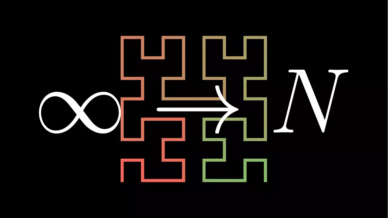
The true Hilbert curve is not any single finite grid traversal, but rather the continuous infinite limit function of recursive pseudo-Hilbert approximations as order approaches infinity. (7:19)
Infinite mathematical objects often serve as clean encapsulations of structural truths about families of finite objects, with finite analogs appearing directly in software and computer engineering. (15:43)

Detailed notes

## Background Published on YouTube by 3Blue1Brown on July 21, 2017, this video investigates space-filling curves and the deeper relationship between infinite and finite mathematics. According to the description, it uses the Hilbert curve to explore how idealized mathematical limits provide practical utility in finite real-world applications.

## TL;DR Using the engineering challenge of designing sight-via-sound software—which translates 2D pixel coordinates into 1D audio frequencies—the video contrasts a simple snake curve with the recursive pseudo-Hilbert curve. While increasing image resolution causes catastrophic spatial shifts under a snake mapping, pseudo-Hilbert curves preserve locality and converge gracefully. Tracing back to Cantor, Peano, and Hilbert's late-19th-century quest to determine if a 1D line could continuously fill a 2D square, the video formalizes curves as continuous functions and defines the true Hilbert curve as their convergent limit. Ultimately, Grant Sanderson shows that infinite mathematical objects are not detached curiosities, but rather elegant, clean tools that encapsulate essential truths about families of finite structures.

## Atmosphere & style The presentation carries 3Blue1Brown's hallmark style: thoughtful, deliberate, and visually mesmerizing. Paired with soft ambient music, the pacing shifts effortlessly from an approachable engineering problem to rigorous definitions of topological continuity and limits. It evokes a genuine sense of intellectual discovery, transforming an ostensibly dry theoretical question about infinity into an intuitive and visually satisfying realization.

## Bulletin - [00:44](https://www.youtube.com/watch?v=3s7h2MHQtxc&t=44s) Space-filling curves provide a practical solution for dimensional reduction problems, such as mapping a 2D image onto a 1D audio frequency spectrum for sight-via-sound sensory substitution software. - [05:45](https://www.youtube.com/watch?v=3s7h2MHQtxc&t=345s) Unlike standard raster or snake scans, pseudo-Hilbert curves preserve spatial locality and remain stable when camera resolutions are upgraded, preventing users from having to relearn frequency-to-pixel associations. - [07:19](https://www.youtube.com/watch?v=3s7h2MHQtxc&t=439s) The true Hilbert curve is not any single finite grid traversal, but rather the continuous infinite limit function of recursive pseudo-Hilbert approximations as order approaches infinity. - [15:43](https://www.youtube.com/watch?v=3s7h2MHQtxc&t=943s) Infinite mathematical objects often serve as clean encapsulations of structural truths about families of finite objects, with finite analogs appearing directly in software and computer engineering.

## Key takeaways - [00:04](https://www.youtube.com/watch?v=3s7h2MHQtxc&t=4s) Mathematics often studies idealized infinite objects, raising the question of how infinite results can be applied to finite, physical engineering contexts. - [00:44](https://www.youtube.com/watch?v=3s7h2MHQtxc&t=44s) Sight-via-sound systems convert 2D visual frames into sound by mapping each pixel to a unique frequency, leveraging neuroplasticity to allow the brain to decode image features. - [02:01](https://www.youtube.com/watch?v=3s7h2MHQtxc&t=121s) The core engineering challenge is dimension reduction from a 2D pixel grid to a 1D frequency line while ensuring that nearby frequencies correspond to spatially adjacent pixels. - [02:01](https://www.youtube.com/watch?v=3s7h2MHQtxc&t=121s) Pseudo-Hilbert curves are recursively generated by subdividing space into quadrants, embedding lower-order curves, and reflecting the bottom quadrants to maintain smooth end-to-end connections. - [05:45](https://www.youtube.com/watch?v=3s7h2MHQtxc&t=345s) Upgrading resolution with a snake curve shifts horizontal coordinates dramatically across the frequency spectrum, destroying established sensory intuition. - [05:45](https://www.youtube.com/watch?v=3s7h2MHQtxc&t=345s) Pseudo-Hilbert curves preserve stability across resolutions because fractional coordinates along the curve converge toward fixed 2D limit positions rather than jumping across the frame. - [07:19](https://www.youtube.com/watch?v=3s7h2MHQtxc&t=439s) Giuseppe Peano discovered the first continuous space-filling curve in 1890, and David Hilbert introduced a geometrically simpler square-subdivision construction in 1891. - [07:19](https://www.youtube.com/watch?v=3s7h2MHQtxc&t=439s) In formal mathematics, a curve is defined as any continuous function mapping a 1D real interval into a space, even if the resulting geometric path contains infinitely many sharp corners. - [07:19](https://www.youtube.com/watch?v=3s7h2MHQtxc&t=439s) No finite pseudo-Hilbert curve fills continuous space on its own; each order is a zero-area path that misses almost all points in a 2D plane. - [09:43](https://www.youtube.com/watch?v=3s7h2MHQtxc&t=583s) Continuity can be framed topologically: shrinking an open neighborhood around an input domain point must allow the smallest bounding circle enclosing the output points to shrink arbitrarily small. - [11:40](https://www.youtube.com/watch?v=3s7h2MHQtxc&t=700s) The true Hilbert curve is rigorously defined as the pointwise limit function of pseudo-Hilbert approximations, which is guaranteed to converge for every input in [0, 1]. - [14:13](https://www.youtube.com/watch?v=3s7h2MHQtxc&t=853s) Proving that the Hilbert curve is a space-filling curve requires confirming three properties: the limit function is well-defined, it is continuous, and it is surjective over the unit square. - [14:13](https://www.youtube.com/watch?v=3s7h2MHQtxc&t=853s) By tiling the infinite plane with squares and connecting spiraling Hilbert curves end-to-end, the positive real line can be continuously mapped to fill all of 2D space. - [15:43](https://www.youtube.com/watch?v=3s7h2MHQtxc&t=943s) The convergence condition required to mathematically define an infinite curve limit is identical to the stability requirement needed to keep sensory mappings consistent across hardware upgrades. - [15:43](https://www.youtube.com/watch?v=3s7h2MHQtxc&t=943s) Infinite mathematical concepts act as a clean lens to encapsulate and prove truths about infinite families of finite objects, mirroring how divergent series relate to two's complement binary arithmetic.

## Detailed walkthrough ### [00:04](https://www.youtube.com/watch?v=3s7h2MHQtxc&t=4s) The Question of Infinite Math in a Finite World

Space-filling curves are celebrated for being visually captivating to animate, but they also serve as a gateway to an enduring philosophical dilemma. Mathematics frequently engages with infinite quantities, often reaching conclusions whose very substance exists purely within an idealized infinite framework. The central problem then becomes: “So the question is, how can these results ever be useful in a finite context?”

Rather than tackling such philosophy in the abstract, it is far more fruitful to inspect a concrete case study first. The investigation begins with a practical software engineering challenge using a Hilbert curve, followed by an exploration of its theoretical origins in infinite mathematics.

```mermaid flowchart LR accTitle: From Infinite Math to Finite Application accDescr: Pipeline showing how the philosophical question of infinity connects to a practical engineering problem. A["Infinite Mathematics (Cantor, Peano, Hilbert)"] --> B["Hilbert Curve (Limit of Curves)"] B --> C["Pseudo-Hilbert Approximations (Orders 1 through 8)"] C --> D["Finite Engineering Application (Sound-to-Sight Mapping)"] ```

---

[00:44](https://www.youtube.com/watch?v=3s7h2MHQtxc&t=44s) Translating Vision to Sound: The Sound-to-Sight Problem

Imagine designing software that allows people to “see with their ears.” The program would capture visual input through a camera and convert it into sound in a meaningful way. This relies on the remarkable plasticity of the human brain, which is capable of extracting spatial intuition even when visual data is scrambled into an entirely different sensory format.

To keep initial prototypes manageable, images are treated at a modest resolution of 256 by 256 pixels, represented as a square grid where each cell corresponds to a single pixel. A straightforward software design maps each individual pixel to a unique sound frequency. The brightness of a pixel determines its amplitude: - A brighter pixel plays its corresponding frequency louder. - A darker pixel plays its frequency quietly or stays silent.

```mermaid flowchart TD accTitle: Sight-via-Sound Architecture accDescr: Flowchart illustrating how a 2D camera image is transformed into an audible audio signal. subgraph InputSpace ["2D Visual Space"] P["Camera Frame (256 × 256 Grid)"] B["Pixel Brightness"] end subgraph AudioEngine ["Mapping Engine"] M["Spatial Curve Mapping (2D to 1D)"] A["Amplitude Modulation (Bright = Loud, Dark = Quiet)"] end subgraph OutputSpace ["1D Audio Space"] F["Superimposed Sound Wave (Cacophony decoded by brain)"] end P --> M B --> A M --> F A --> F ```

When all pixels are processed simultaneously, the ear receives an intricate overlay of thousands of frequencies sounding at once. While it initially resembles a cacophonous wall of noise, the brain can gradually learn to parse the dominant frequencies corresponding to bright visual regions into a coherent mental image.

---

[02:01](https://www.youtube.com/watch?v=3s7h2MHQtxc&t=121s) Dimension Reduction: Snake Curves vs. Hilbert Curves

The fundamental mathematical hurdle in sight-via-sound software is dimensional mismatch: pixel space is two-dimensional, whereas frequency space is strictly one-dimensional. Although human neuroplasticity might eventually decipher a completely random mapping, software should ideally align with existing sensory intuitions. In particular, frequencies that sit close to one another in audio space should correspond to pixels that sit close to one another in physical 2D space, ensuring that auditory imprecision translates to localized spatial approximations rather than wildly scattered errors.

This mapping can be visualized by weaving a continuous thread through every pixel in the grid and then pulling the thread taut into a straight one-dimensional frequency line. The most intuitive path is a serpentine track that traverses one row at a time, alternating left-to-right and right-to-left as it climbs the grid—resembling a game of Snake. However, when consulted on this design, a mathematician friend immediately proposes an alternative: “When you tell your mathematician friend about this idea, she says, why not use a Hilbert curve?”

```mermaid flowchart LR accTitle: Curve Weaving Process accDescr: Conceptual workflow showing how 2D pixels are serialized onto a 1D line of frequencies. A["2D Pixel Grid (x, y)"] -->|"Weave Continuous Path"| B["Single Thread Traversal"] B -->|"Unravel & Stretch Straight"| C["1D Frequency Spectrum (f)"] ```

A true Hilbert curve is a singular limit object, but understanding it requires constructing an infinite family of approximations known as "pseudo-Hilbert curves": - **Order-1 pseudo-Hilbert curve:** Subdivides a square into a 2×2 grid and connects the center of the lower-left quadrant to the upper-left, then across to the upper-right, and finally down to the lower-right. - **Order-2 pseudo-Hilbert curve:** Subdivides the area into a 4×4 grid. Each quadrant contains an order-1 mini-curve. To avoid awkward leaps between quadrants, the mini-curves in the lower-left and lower-right quadrants are reflected/rotated so their entry and exit points connect tip-to-tail smoothly. - **Order-3 pseudo-Hilbert curve:** Subdivides the area into an 8×8 grid, embedding an order-2 curve inside each quadrant with appropriate reflections in the lower quadrants to preserve end-to-end connections. - **Order-8 pseudo-Hilbert curve:** Continues this recursive expansion up to a 256×256 grid, precisely matching the target camera resolution.

---

[05:45](https://www.youtube.com/watch?v=3s7h2MHQtxc&t=345s) The Resolution Upgrade Paradox

While pseudo-Hilbert curves are visually striking, their practical superiority over the simple snake curve becomes obvious when considering hardware upgrades. Suppose the software succeeds, gains a global user base, and prompts an engineering update that increases camera resolution from 256×256 to 512×512 pixels.

Under the snake curve, increasing resolution causes catastrophic spatial shifts across the frequency spectrum. A frequency located halfway along the line will still land roughly halfway up the vertical axis, but its horizontal coordinate can swing radically from one side of the image to the other. Consequently, an upgrade would wipe out users' hard-won sensory intuition: “This means everyone using your software would have to re-learn how to see with their ears, since the original intuitions of which points in space correspond to which frequencies no longer apply.”

In contrast, the pseudo-Hilbert curve preserves locality across orders: - As the curve's order increases, the position mapped to any given fractional point along the 1D line moves less and less. - Points simply converge toward a precise coordinate in 2D space. - Users only need to fine-tune their existing perceptual model rather than retraining their brains from scratch.

---

[07:19](https://www.youtube.com/watch?v=3s7h2MHQtxc&t=439s) Historical Origins and the Nature of Space-Filling Curves

The uncanny perfection of the Hilbert curve for this modern engineering problem raises the question of why it was invented in the first place. Near the close of the 19th century, triggered by Georg Cantor's groundbreaking discoveries regarding infinite sets, mathematicians wrestled with whether an infinitely thin, zero-area 1D line could pass through every single point in an infinite, continuous 2D area.

Prior to 1890, common intuition held that such a mapping was impossible. Giuseppe Peano shocked the mathematical world in 1890 by constructing the first continuous space-filling curve, and in 1891, David Hilbert devised a geometrically simpler variation based on square subdivisions. Although these curves specifically fill a unit square, filling the entirety of infinite 2D space becomes trivial once a single bounded square can be filled.

```mermaid flowchart TD accTitle: Historical Emergence of Space-Filling Curves accDescr: Timeline diagram highlighting the developments leading to Hilbert's discovery. C["Cantor's Set Theory & Infinity (Late 19th Century)"] --> P["Peano Discovers First Space-Filling Curve (1890)"] P --> H["Hilbert Introduces Simpler Geometric Curve (1891)"] H --> Modern["Fractal Geometry & Modern Applications (Dimension Reduction)"] ```

Mathematical conventions often create confusion here. In formal mathematics, the word "curve" applies to any continuous parameterized line through space, even if it contains infinitely many sharp, jagged corners: “A better name might be something like space-filling fractal, which some people do use, but hey, it's math, so we live with bad terminology.”

Crucially, no finite pseudo-Hilbert curve actually fills space. If one zooms in on a single pixel in a continuous plane, a pseudo-Hilbert curve traces merely a zero-area strand through it, missing virtually all of the infinitely many points in that region. The true, genuine Hilbert curve is not any discrete step in the sequence, but rather the infinite mathematical limit of the pseudo-Hilbert curves as the order approaches infinity.

---

[09:43](https://www.youtube.com/watch?v=3s7h2MHQtxc&t=583s) Formalizing Curves as Functions and the Definition of Continuity

To establish what this infinite limit actually is, curves must be formalized as continuous functions. Specifically, a plane-filling curve is a function mapping a 1D real-number interval into 2D coordinate space: $$\gamma: [0, 1] \to [0, 1] \times [0, 1]$$ The input is a single scalar $t \in [0, 1]$ representing a position along the thread, and the output is a coordinate pair $(x, y)$.

As concrete examples of how finite pseudo-Hilbert curves act as functions: - An order-2 pseudo-Hilbert function maps input $0.3$ to output coordinates $(0.125, 0.75)$. - An order-3 pseudo-Hilbert function maps the same input $0.3$ to output coordinates $(0.0758, 0.6875)$.

The defining property separating a legitimate curve from an arbitrary scrambling of points is continuity. The core intuition is straightforward: “The intuition behind continuity is that you don't want the output of your function to suddenly jump at any point when the input is only changing smoothly.”

To make this mathematically rigorous, consider an input point $a$ and its corresponding output location $b = f(a)$: 1. Construct an open circle (or interval) centered around $a$ in the input domain. 2. Observe the set of output points produced by mapping every point inside that input neighborhood through the function. 3. Draw the smallest bounding circle centered at $b$ in the output space that fully encloses all those mapped outputs. 4. Varying the radius of the input circle directly controls the size of the resulting bounding circle in the output space, laying the groundwork for the formal topological limit definition of continuity.

[11:40](https://www.youtube.com/watch?v=3s7h2MHQtxc&t=700s) Formalizing Continuity and Defining the True Hilbert Curve

To understand what a curve actually is in rigorous mathematics, one must look at continuity through the lens of bounding circles. If a function jumps at a point $a$, drawing a circle around $a$, inspecting the mapped outputs of all the inputs inside that neighborhood, and trying to enclose them within the smallest possible circle centered at output $b$ reveals a fundamental barrier. No matter how much you shrink the input circle around $a$, the corresponding output circle around $b$ cannot shrink past the size of that jump. Grant Sanderson explains that “the function is discontinuous at $a$ if there's any lower bound on the size of this circle that surrounds $b$.” Conversely, if the circle surrounding $b$ can be made arbitrarily small simply by choosing sufficiently small neighborhoods around $a$, the function is continuous at that point. A function as a whole earns the title of continuous only if it meets this standard across every single input point.

```mermaid flowchart TD accTitle: Hilbert Curve Limit Process accDescr: Diagram showing how a single input maps through successive pseudo-Hilbert curves to a convergent limit point. subgraph InputSpace ["1D Domain"] X["Input x in [0, 1] (e.g., 0.3)"] end subgraph Approximations ["Successive Pseudo-Hilbert Orders"] H1["H₁(x)"] H2["H₂(x)"] H3["H₃(x)"] Hn["Hₙ(x)"] end subgraph OutputLimit ["2D Range"] Lim["Point (x, y) = lim Hₙ(x)"] end X --> H1 X --> H2 X --> H3 X --> Hn H1 -.-> H2 H2 -.-> H3 H3 -.-> Hn Hn --> Lim ```

With continuity established, the true Hilbert curve can be rigorously defined using a unique property of pseudo-Hilbert approximations. If you pick any fixed input value between $0$ and $1$ (such as $0.3$) and evaluate each successive pseudo-Hilbert curve function at that exact value, the outputs do not wander indefinitely. As the order increases, the resulting points in 2D space stabilize and converge toward a specific coordinate. This behavior is distinctly absent in simple snake curves or typical pixel-scanning sequences, where outputs jump wildly from left to right across increasing resolutions without ever settling. Because every input produces a sequence of outputs that is guaranteed to converge, the true Hilbert curve function $H(t)$ is formally defined as the limit of these pseudo-Hilbert outputs.

- Continuity requires that output circles can be made as small as desired by restricting input neighborhood size. - A sequence of pseudo-Hilbert functions evaluated at any point in $[0, 1]$ always converges to a single 2D coordinate. - Snake curves fail to produce a limit function because output points oscillate erratically across higher resolutions.

[14:13](https://www.youtube.com/watch?v=3s7h2MHQtxc&t=853s) The Three Proof Obligations and Filling All of Space

Although Sanderson does not walk through the complete formal proof in the video, he lays out the three essential checkpoints required to demonstrate that this construction genuinely yields a space-filling curve:

1. **Well-defined function**: Prove that for every input in $[0, 1]$, the sequence of pseudo-Hilbert curve outputs truly converges to a unique limit. 2. **Curve (continuity)**: Prove that the resulting limit function is continuous across the entire unit interval. 3. **Space-filling property**: Prove that every single point within the 2D unit square is hit by the function (i.e., the mapping is surjective).

Grant encourages viewers to tackle these challenges themselves, offering the reassuring “Spoiler alert, all three of these facts turn out to be true.”

Once the unit square is filled, the construction can be extended to cover all of 2-dimensional space. By tiling the infinite plane with squares and connecting consecutive Hilbert curves in an outward spiraling pattern—bridging the end of one tile to the start of the next with a short connecting segment if necessary—the entire positive real number line can be mapped surjectively onto $\mathbb{R}^2$. Interval $[0, 1]$ fills the first tile, $[1, 2]$ fills the second, and so on. As Sanderson reflects on the philosophical weight of the result: “A line, the platonic form of thinness itself, can wander through an infinitely extending and richly dense space and hit every single point.”

[15:43](https://www.youtube.com/watch?v=3s7h2MHQtxc&t=943s) Infinite Math as a Clean Lens for Finite Reality

The stabilizing behavior that makes the infinite Hilbert curve mathematically sound is the exact same trait that makes pseudo-Hilbert curves ideal for practical engineering, such as translating video frames into soundscapes. For sensory substitution, spatial stability means that increasing camera resolution does not scramble the frequency mapping or force a user to relearn how to interpret auditory sensations. For pure mathematicians, that same stability is the precise condition needed for a sequence of functions to converge to a well-defined limit.

Sanderson highlights that this bridge between the finite and the infinite is a recurring principle throughout mathematics rather than a rare coincidence. A related example, noted by viewers of his earlier video on inventing math, is the link between the divergent geometric series of powers of two ($\sum 2^n$) and the way negative one ($-1$) is represented in binary computer systems via two's complement. The utility does not stem from taking infinite infinities literally in physical hardware, but rather because “the same patterns and constructs that are used to define and prove infinite facts have finite analogs, and these finite analogs are directly useful.”

Furthermore, theorems concerning infinite mathematical objects are frequently equivalent to rigorous statements about entire families of finite objects. If an engineer were to formalize the requirement that an image-to-audio curve must remain stable as sensor resolutions increase, they would naturally recreate the formal epsilon-delta definition of a curve limit. Sanderson summarizes the overarching takeaway:

> “In fact, a statement about some infinite object, whether that's a sequence or a fractal, can usually be viewed as a particularly clean way to encapsulate a truth about a family of finite objects.”

He urges viewers to keep an open mind whenever a mathematical concept appears detached from the physical world. Looking beneath the surface reveals core mechanics that can unlock unexpected solutions—whether that means finding robust representations of numbers through divergent sums or learning how to see with your ears through the geometry of space-filling curves.

## Notable quotes > [14:13](https://www.youtube.com/watch?v=3s7h2MHQtxc&t=853s) A line, the platonic form of thinness itself, can wander through an infinitely extending and richly dense space and hit every single point. — Grant Sanderson

> [15:43](https://www.youtube.com/watch?v=3s7h2MHQtxc&t=943s) In fact, a statement about some infinite object, whether that's a sequence or a fractal, can usually be viewed as a particularly clean way to encapsulate a truth about a family of finite objects. — Grant Sanderson

> [09:43](https://www.youtube.com/watch?v=3s7h2MHQtxc&t=583s) The intuition behind continuity is that you don't want the output of your function to suddenly jump at any point when the input is only changing smoothly. — Grant Sanderson

## Mentioned David Hilbert, Giuseppe Peano, Georg Cantor, Grant Sanderson, 3Blue1Brown, Terry Tao, Vincent Rubinetti, Kevin Pluck, Omer Tuchfeld

## Video description Space-filling curves, and the connection between infinite and finite math. Help fund future projects: https://www.patreon.com/3blue1brown An equally valuable form of support is to simply share some of the videos. Home page: https://www.3blue1brown.com

Supplement with more space-filling curve fun: https://youtu.be/RU0wScIj36o

For more information on sight-via sound, this paper involving rewiring a ferret's retinas to its auditory cortex is particularly thought-provoking: http://phy.ucsf.edu/~houde/coleman/sur2.pdf

Alternatively, here is the NYT summary: https://goo.gl/qNuc14

Also, check out this excellent podcast on Human echolocation: https://goo.gl/23f4Yh

For anyone curious to read more about the connections between infinite and finite math, consider this Terry Tao blog post: https://goo.gl/NZ4yrW

Lion photo by Kevin Pluck

Music by Vincent Rubinetti: https://vincerubinetti.bandcamp.com/album/the-music-of-3blue1brown

Thanks to these viewers for their contributions to translations Hebrew: Omer Tuchfeld

------------------

3blue1brown is a channel about animating math, in all senses of the word animate. And you know the drill with YouTube, if you want to stay posted on new videos, subscribe, and click the bell to receive notifications (if you're into that).

Various social media stuffs: Website: https://www.3blue1brown.com Twitter: https://twitter.com/3Blue1Brown Patreon: https://patreon.com/3blue1brown Facebook: https://www.facebook.com/3blue1brown Reddit: https://www.reddit.com/r/3Blue1Brownm/r/3Blue1Brown

[Source](https://www.youtube.com/watch?v=3s7h2MHQtxc)

中文简报

希尔伯特曲线可防止图像转音频系统中的空间偏移定义无限空间填充曲线的收敛条件，提供了在分辨率升级时保持有限感官替代映射稳定所需的精确数学保障。视频以设计“以声代视”软件（将二维像素坐标转化为一维音频频率）的工程挑战为例，对比了简单的蛇形曲线与递归伪希尔伯特曲线。虽然在蛇形映射下提高图像分辨率会导致灾难性的空间偏移，但伪希尔伯特曲线能保留局部性并优雅地收敛。追溯到19世纪晚期康托尔、皮亚诺和希尔伯特关于一维线是否能连续填满二维正方形的探索，视频将曲线形式化为连续函数，并将真正的希尔伯特曲线定义为其收敛极限。最终，格兰特·桑德森表明，无限数学对象并非脱离实际的奇谈怪论，而是优雅明晰的工具，概括了有关有限结构族的本质真理。空间填充曲线为降维问题提供了切实可行的解决方案，例如在以声代视感官替代软件中将二维图像映射到一维音频频谱上。 (0:44) 与标准的光栅或蛇形扫描不同，伪希尔伯特曲线能保留空间局部性，并在相机分辨率升级时保持稳定，避免用户重新学习频率与像素之间的关联。 (5:45) 真正的希尔伯特曲线并不是任何单一的有限网格遍历，而是当阶数趋于无穷大时，递归伪希尔伯特逼近的连续无限极限函数。 (7:19) 无限数学对象通常清晰地概括了有关有限对象族的结构真理，其有限模拟则直接应用于软件和计算机工程之中。 (15:43)

Reading summary

Grant Sanderson argues that infinite mathematical constructs are directly useful in finite engineering because statements about infinite limits cleanly capture the stability and convergence properties needed across families of finite systems. Dimension Reduction in Sensory Substitution (0:44) Developing software that allows users to 'see with their ears' requires translating a two-dimensional visual grid into a one-dimensional audio spectrum. In a prototype mapping a 256 by 256 pixel camera feed to distinct sound frequencies, brightness modulates amplitude so that prominent visual objects register as dominant tones. The core engineering hurdle is dimension reduction: the mapping must preserve spatial locality so that adjacent frequencies correspond to neighboring pixels, ensuring that auditory imprecision translates to minor spatial blur rather than disjointed noise. Resolution Scaling and Locality Preservation (5:45) A naive serpentine snake curve traverses the grid row by row, but upgrading camera resolution from 256 by 256 to 512 by 512 pixels causes drastic horizontal shifts across the frequency line. Because points along the curve swing wildly across the visual field under higher resolutions, users would be forced to relearn spatial interpretation after every hardware update. In contrast, recursive pseudo-Hilbert curves subdivide space into quad-trees with rotated mini-curves, ensuring that points settle progressively into localized clusters. As resolution increases, spatial coordinates converge toward fixed positions, allowing users to preserve and fine-tune their perceptual habits. Formal Continuity and the Infinite Limit (11:40) No finite pseudo-Hilbert curve fills space; each traces a zero-area path that misses most points in a continuous region. The true Hilbert curve, introduced geometrically in 1891 following Giuseppe Peano's 1890 discovery, exists only as the infinite limit of these successive approximations. Formalized as a continuous function from the unit interval to the unit square, continuity requires that shrinking the input neighborhood guarantees an arbitrarily small bounding circle around the output point. While snake curves oscillate erratically without settling, pseudo-Hilbert sequences evaluated at any input point converge to a unique coordinate, yielding a continuous, surjective curve that can be extended across all two-dimensional space. Infinite Theorems as Finite Blueprints (15:43) The mathematical stability that allows the Hilbert curve to converge to a well-defined infinite limit is identical to the engineering requirement preventing sensory distortion during resolution upgrades. Sanderson notes that this reflects a widespread pattern: an infinite theorem often serves as a clean lens encapsulating truths about an entire family of finite objects. A similar correspondence appears between divergent geometric series of powers of two and the representation of negative one in computer two's complement arithmetic, illustrating that theoretical infinity provides practical templates for finite computation. While physical hardware remains bounded by finite constraints, Sanderson concludes that abstract mathematics should not be dismissed as impractical; the constructs used to resolve infinite paradoxes directly furnish the stability criteria needed in real-world system design.

精炼阅读摘要

Grant Sanderson（3Blue1Brown）指出，数学中关于无限对象的严谨结论看似脱离现实，但实质上提供了一种极其精炼的理论透镜，能够完整概括与统一整族有限对象的共性规律与工程稳定性。感官替代中的降维挑战与蛇形扫描缺陷 (2:01) 在设计让视障人士“以耳代眼”的感官替代软件时，工程核心在于将摄像头捕捉的二维图像转化为人耳可识别的一维音频信号。该系统依托人类大脑的可塑性，将256×256像素网格中的每个像素映射到独特的声音频率上，并以像素亮度控制振幅，使高亮区域的声音更大，最终叠加成复杂的复合声波由大脑解析出空间图像。该设计的核心数学瓶颈在于维度不匹配：图像属于二维物理空间，而声音频率属于严格的一维空间。为了符合人类感知直觉，映射算法必须保持空间局部性，即频率上相近的声音必须对应物理空间中邻近的像素，从而确保听觉上的轻微误差只产生局部空间模糊，而非全局错乱。最直观的降维方案是类似贪吃蛇的蛇形走线，即逐行交替扫描像素点并拉直为一维频率线。然而当硬件升级将分辨率提升至512×512时，蛇形走线会导致灾难性的空间跳跃：处于频率中点的像素虽然在纵向仍居中，但横向位置会跨越整幅图像左右剧烈摆动。这种不稳定性会彻底摧毁用户已建立的听觉空间直觉，迫使其重新训练大脑。伪希尔伯特曲线的局部性与升级稳定性 (5:45) 为了解决蛇形映射在分辨率提升时的失效问题，数学家提出了伪希尔伯特曲线方案。该曲线通过递归四叉树进行网格划分，并对下半部分的子曲线进行旋转和翻转，以保证曲线首尾连续平滑拼接。阶数为1的曲线遍历2×2网格，阶数为2的曲线遍历4×4网格，直至阶数达到8时精准覆盖256×256像素。伪希尔伯特曲线在空间降维中展现出显著优势：它能最大程度保留邻域特征，一维序列中相邻的点在二维空间内高度聚类于同一象限内，避免了边缘处的长距离跳跃。更为关键的是其跨分辨率的稳定性。当算法从低阶伪希尔伯特曲线升级至更高阶时，一维线上任意特定比例位置所对应的二维坐标位移幅度会越来越小，并逐步收敛至确定的空间点。这意味着在硬件升级时，用户此前形成的听觉感知直觉不会被推翻，仅需微调即可适应更高精度的图像输出。空间填充曲线的历史起源与连续性极限 (9:43) 希尔伯特曲线最初并非诞生于工程需求，而是源于19世纪末纯粹数学对无穷维度的哲学探讨。在康托尔（Georg Cantor）创立集合论后，数学界开始质疑一条零面积的一维连续直线是否可能完全填满连续的二维平面。1890年皮亚诺（Giuseppe Peano）构造出首个连续空间填充曲线，打破了传统直觉；1891年希尔伯特（David Hilbert）提出了基于正方形细分的几何简化版本。在现代数学中，“曲线”被严格形式化为从一维实数区间映射到二维空间的连续函数。为界定函数的连续性，数学上要求对于输入点邻域内的所有点，其输出点构成的最小外接圆能够随着输入范围的缩小而收敛到任意小；若存在无法缩小的跳跃下界，则函数不连续。严格意义上的真正希尔伯特曲线并非任何离散的有限阶曲线，因为任何有限阶曲线在连续平面中都仅是零测度的线段，其本质是当阶数趋向无穷大时伪希尔伯特函数序列的极限。该极限被证明满足三大严格条件：每个输入点收敛至唯一定义的极限、极限函数处处连续，且映射具有填满单位正方形的满射性。通过将该正方形向外螺旋拼接，整条正实数轴亦可满射至整个二维欧氏平面。无限数学是刻画有限对象规律的理论透镜 (15:43) Sanderson强调，无限希尔伯特曲线在数学上收敛所依赖的内在稳定性，恰恰是在工程实践中伪希尔伯特曲线能够平滑支持分辨率升级的物理依据。数学家界定无限对象极限所需的收敛条件，与工程师为了避免用户重新训练而设定的空间平差标准完全等价。这种无限与有限之间的呼应在数学中屡见不鲜：例如计算机底层使用二进制补码表示负一（-1）的机制，在结构上完全映射了公比为2的发散几何级数和。纯数学对于无限对象或分形的定理，其真正的现实价值在于提供了一种极为纯粹的语言，用于封装整族有限近似对象的共同规律。如果工程师试图从零推导出一套保证多分辨率平稳过渡的数学框架，最终也将自然重建出微积分与拓扑学中的ε-δ极限定义。因此，看似脱离物理现实的抽象数学概念，其深层结构往往蕴含着解决现实复杂工程难题的关键钥匙。综上所述，无限数学的实用性并非源于物理世界中存在真正的无穷实体，而在于其严谨的极限工具为有限工程系统提供了统一的稳定性度量与结构范式。以希尔伯特曲线为代表的数学结构，不仅消解了维度降维中的失真难题，也印证了抽象理论在有限现实应用中的深刻映照。

Detailed notes — zh

## Background 该内容由数学科普频道 3Blue1Brown 于 2017 年 7 月 21 日在 YouTube 平台发布。视频简介指出，本期主题围绕空间填充曲线展开，深入探讨了无限数学与有限数学之间的内在联系，并附带了声音替代视觉实验及相关数学拓展资料。 ## TL;DR 视频首先通过一个“用声音代替视觉”的工程设想切入，探讨如何将二维像素图像降维映射到一维声音频率上，并对比了贪吃蛇曲线与伪希尔伯特曲线在分辨率升级时的表现。随后，内容追溯至 19 世纪末康托尔、皮亚诺与希尔伯特关于空间填充曲线的纯数学探索，借助实分析中极限与连续性的严格几何定义，阐释了真正的希尔伯特曲线是如何作为伪曲线族的极限而填满整个空间的。最后，视频深刻揭示了无限数学与有限现实之间的对偶关系，指出关于无限对象的优美定理本质上是对有限现实模式的精妙封装，能为实际工程问题提供深层指导。 ## Atmosphere & style 整部作品延续了 3Blue1Brown 标志性的从容、优雅与思辨质感。叙事从一个极具科幻感的具体工程问题自然过渡到纯粹拓扑学的深水区，由浅入深，层层递进。生动形象的几何动画化解了严格分析学定义的枯燥，让观众在直面数学极限与连续性的严谨逻辑时，油然而生一种对无限之美与现实实用性奇妙交融的智性震撼。 ## Bulletin - [03:19](https://www.youtube.com/watch?v=3s7h2MHQtxc&t=199s) 希尔伯特曲线并非单条曲线，而是一个无限曲线族的收敛极限；其构造成功打破了“零面积一维线无法填满二维连续空间”的历史直觉。 - [05:45](https://www.youtube.com/watch?v=3s7h2MHQtxc&t=345s) 在感官替代工程（如将摄像头画面转为音频）中，伪希尔伯特曲线具备优异的局部邻域保持性，可在硬件分辨率倍增时避免频率与空间方位的剧烈偏移。 - [15:43](https://www.youtube.com/watch?v=3s7h2MHQtxc&t=943s) 纯数学中对“曲线序列存在极限”的分析学证明，在工程实践中直接等价于高分辨率网格遍历时算法结构的稳定性与向后兼容性。 - [16:43](https://www.youtube.com/watch?v=3s7h2MHQtxc&t=1003s) 无限数学的实用价值并不在于无限结果本身，而在于定义与证明无限事实所沉淀出的理论构造，往往可以直接映射为有限现实系统的核心算法。 ## Key takeaways - [00:04](https://www.youtube.com/watch?v=3s7h2MHQtxc&t=4s) 探讨无限数学现实意义的哲学命题，可以通过希尔伯特曲线在有限工程应用与纯粹数学极限之间的映射关系得到清晰展现。 - [00:44](https://www.youtube.com/watch?v=3s7h2MHQtxc&t=44s) 借助人脑的高度可塑性，可开发“用耳朵看世界”的感官替代系统，通过将二维图像像素降维映射到一维声波频率并混合播放来实现空间感知。 - [02:00](https://www.youtube.com/watch?v=3s7h2MHQtxc&t=120s) 为了契合人类听觉的原生直觉，从一维频率到二维空间的映射必须具备良好的局域保持性，即彼此接近的频率应对应像素空间中紧密相邻的区域。 - [05:45](https://www.youtube.com/watch?v=3s7h2MHQtxc&t=345s) 传统的逐行“贪吃蛇曲线”虽能遍历网格，但若遇到传感器分辨率翻倍（如从 256×256 升至 512×512），同一频率对应的空间坐标会发生剧烈左右横跳，破坏认知一致性。 - [03:19](https://www.youtube.com/watch?v=3s7h2MHQtxc&t=199s) 通过对子象限进行几何翻转与首尾相连所构建的伪希尔伯特曲线，随着阶数提升，各点在二维坐标上的摆动幅度急剧缩小，表现出高度的收敛稳定性。 - [07:19](https://www.youtube.com/watch?v=3s7h2MHQtxc&t=439s) 历史上皮亚诺与希尔伯特提出的空间填充曲线，打破了 19 世纪末主流学界关于“一维连续线绝不可能覆盖二维连续空间中每一个点”的朴素认知。 - [08:43](https://www.youtube.com/watch?v=3s7h2MHQtxc&t=523s) 任何有限阶的伪希尔伯特曲线本质上都只是面积为零的折线；真正的希尔伯特曲线被严格定义为该函数序列在 n 趋于无穷时的逐点极限。 - [09:43](https://www.youtube.com/watch?v=3s7h2MHQtxc&t=583s) 数学上曲线的严密定义依赖于连续性，即在输入端选取足够小的邻域圆时，输出端对应的包含圆能够被约束至任意微小。 - [11:40](https://www.youtube.com/watch?v=3s7h2MHQtxc&t=700s) 由于伪希尔伯特曲线序列在定义域 [0, 1] 上的每一点都严格收敛，由此生成的极限映射函数是一个良定义（well-defined）的连续函数。 - [14:13](https://www.youtube.com/watch?v=3s7h2MHQtxc&t=853s) 希尔伯特曲线是严格意义上的满射，能精确穿过单位正方形内的每一个连续点，且可通过螺旋瓷砖拼接延展至整个二维平面。 - [15:43](https://www.youtube.com/watch?v=3s7h2MHQtxc&t=943s) 工程应用中要求“分辨率提升时坐标保持稳定”的形式化表述，在分析学意义上完全等价于无穷曲线序列存在极限的收敛性条件。 - [16:43](https://www.youtube.com/watch?v=3s7h2MHQtxc&t=1003s) 研究无限数学的真正力量在于，用于证明无限事实的思维框架与结构模式，往往能够直接启发并解决有限现实世界中的工程技术难题。 ## Detailed walkthrough ### [00:04](https://www.youtube.com/watch?v=3s7h2MHQtxc&t=4s) 空间填充曲线与无限数学的现实意义数学经常与无限量（infinite quantities）打交道，有时其研究结果的本质只在无限世界中才具有实际意义。这就引出了一个核心的哲学追问：这类结果究竟如何能在有限的现实语境中发挥作用？正如主讲人所言：“As with all philosophizing, this is best left to discuss until after we look at the concrete case and the real math.”（正如所有的哲学思考一样，这最好留到我们看完具体案例和真正的数学之后再讨论。）为了探讨这一命题，讨论先从希尔伯特曲线（Hilbert curve）的一个实际应用场景切入，随后追溯它在无限数学中的起源。 ### [00:44](https://www.youtube.com/watch?v=3s7h2MHQtxc&t=44s) 用声音代替视觉：将二维像素映射到一维频率设想编写一套能够让人们“用耳朵看见”的软件：系统从摄像头获取图像数据，并将其以一种有意义的方式转化为声音。人类的大脑具有高度的可塑性，即便原始数据被重构打乱成不同的感官输入格式，也依然有可能建立起视觉直觉。为了便于进行早期实验，可以先将输入图像降为较低的分辨率（例如 256×256 像素），并用正方形网格来表示图像，每个方格对应一个像素。实现该软件的一种直接方案，是为每一个像素指定一个唯一的声波频率（frequency）： - 像素亮度越高，其对应的频率在播放时的音量就越大。 - 像素越暗，该频率的声音就越微弱。 - 同时播放所有像素的频率时，初听起来会是一堆互相重叠、极度杂乱的刺耳噪音（cacophonous mess），但随着大脑逐步适应，它便能够解析其中包含的空间信息。 ```mermaid flowchart LR accTitle: 声音替代视觉的映射流程 accDescr: 展示从摄像头获取图像、将二维像素降维映射到一维频率线并合成音频的过程 subgraph Vision["视觉输入"] Cam["摄像头采集 256×256 图像"] Grid["二维正方形像素网格"] end subgraph Mapping["空间降维映射"] Curve["编织曲线遍历所有像素"] Line["拉直为一维频率空间"] end subgraph Audio["音频输出"] Sound["亮度对应音量大小"] Ear["多频率混合播放至耳机"] end Cam --> Grid Grid --> Curve Curve --> Line Line --> Sound Sound --> Ear ``` 该系统面临的核心几何难点在于：**像素空间是二维的，而声音的频率空间是一维的**。虽然理论上可以使用随机映射（反正依赖大脑去强行理解混乱数据），但若能借助人类对声音的原生直觉会好得多。反向来看，从频率空间映射回像素空间时，彼此接近的频率理应对应像素空间中相互靠拢的区域。这样一来，即便人耳难以精细分辨两个极其相近的频率，它们至少也指向空间中的大致同一位置。为此，必须设计一条穿过所有像素的线条，将每个像素固定在线上并将其完全拉直，以此建立起从二维像素到一维频率的连续映射。 ### [03:19](https://www.youtube.com/watch?v=3s7h2MHQtxc&t=199s) 贪吃蛇曲线与伪希尔伯特曲线的几何构造最直观的穿线方式是逐行遍历，随着在像素空间向上推进，线条在每一行左右交替折返。这种轨迹就像玩得很好的一局贪吃蛇游戏，因此可称之为“贪吃蛇曲线”（Snake Curve）。然而，如果向数学家朋友请教，她会建议使用希尔伯特曲线。当被追问这到底是什么时，数学家先是犹豫了一下，然后澄清道：“So it's not a curve, but an infinite family of curves.”（所以它不是单单一阶曲线，而是一个无限的曲线族。）为了解释清楚，她拿出纸笔，先画出了一系列被她称为“伪希尔伯特曲线”（pseudo-Hilbert curves）的几何迭代图形： 1. **一阶伪希尔伯特曲线（Order-one）**：将正方形划分为 2×2 的网格，线条依次连接左下象限中心、左上象限中心、右上象限中心，最后落至右下象限中心（呈现一个开口朝下的倒“U”形）。 2. **二阶伪希尔伯特曲线（Order-two）**：为了让曲线在跨越象限时先把象限内部填满，将正方形进一步细分为 4×4 的网格。在每个象限内部各画出一个微缩版的一阶曲线。如果直接连接，从左下曲线的末尾到左上曲线的开头、以及从右上到右下都需要尴尬的远距离跳跃；因此，将左下与右下的微型曲线做对称翻转（flip），使各个拐角处的连接距离变得最短。 3. **三阶及更高阶伪希尔伯特曲线（Order-three & Higher）**：将正方形细分为 8×8 的网格，在四个象限中各放入一个二阶伪希尔伯特曲线，适度翻转左下与右下象限的曲线形态，再首尾相连（tip to tail）。对于实验中使用的 256×256 像素矩阵，正好对应使用**八阶伪希尔伯特曲线**（$2^8 \times 2^8$）。这种通过曲线贯穿每一个像素的做法，在数学上等价于建立了一个从像素空间到频率空间的单射函数。 ### [05:45](https://www.youtube.com/watch?v=3s7h2MHQtxc&t=345s) 分辨率升级场景下的局域保持优势使用伪希尔伯特曲线而非贪吃蛇曲线的根本优势，体现在硬件升级的场景中。假设这套视听软件投入使用且大获成功，全世界的用户都在借助耳机建立听觉视觉直觉，此时开发者发布了固件升级，将摄像头分辨率从 256×256 提升到 512×512： - **贪吃蛇曲线的崩溃**：提升分辨率后，频率线上的许多固定点会瞬间跳跃到像素空间中完全不同的位置。以频率线正中间（50% 处）的点为例，无论分辨率如何变化，它的纵向高度虽然始终保持在大约中央位置，但在横向（左右）的位置上，从 256×256 变到 512×512 时会发生剧烈的左右偏移。这意味着所有老用户必须全部“重新学习”如何用耳朵看世界，因为频率与空间方位的对应记忆被彻底打破。 - **希尔伯特曲线的稳定性**：随着伪希尔伯特曲线阶数的提高，频率线上任意一个给定的点在二维空间中的摆动幅度会越来越小，它只是在“逼近”一个更加具体且收敛的空间坐标。用户不需要颠覆原有的认知经验，只需要在原有听觉记忆的基础上微调直觉即可。 ### [07:19](https://www.youtube.com/watch?v=3s7h2MHQtxc&t=439s) 空间填充曲线的起源与真正定义这种近乎完美的数学匹配并非巧合。在 19 世纪末，受康托尔（Cantor）关于无穷大研究的冲击，数学界开始探究是否可能找到一种从一维直线到二维空间的连续映射，使得这条线能够精确穿过空间中的“每一个点”。必须明确的是，这指的并不是有限离散的像素网格，而是由无限个点组成的**连续空间**（continuous space）。其目标是让一条自身宽度无限细、面积严格为零的线，完完全全铺满具有无限面积的空间。在 1890 年之前，主流观点几乎一致认为这是天方夜谭，直到皮亚诺（Peano）发现了第一条空间填充曲线（space-filling curve）。随后在 1891 年，希尔伯特（Hilbert）提出了自己构造更为简单、几何直观更清晰的空间填充曲线。在数学术语中，即使一条线全是尖锐的锯齿拐角，数学家也依然称其为“曲线”（curve），这种命名在空间填充曲线的语境下尤为反直觉，因为这类曲线本质上几乎全由尖角构成，更恰当的叫法或许是“空间填充分形”（space-filling fractal）。任何阶数的伪希尔伯特曲线都**不是**真正的空间填充曲线。只要在一个像素上无限放大，就会发现曲线在连续空间中仅仅穿过了该区域面积为零的一小条细丝，绝没有填满其内部所有的点。真正的希尔伯特曲线是这一系列伪希尔伯特曲线的**极限**（limit）。 ### [09:43](https://www.youtube.com/watch?v=3s7h2MHQtxc&t=583s) 连续性的数学严格定义与局部邻域要严格定义这一极限，必须首先将曲线形式化为数学函数：即以区间 $[0, 1]$ 之间的一个实数作为输入，输出平面上的一个数对 $(x, y)$。输入值对应线上的具体位置，输出值对应二维平面的坐标： - 在二阶伪希尔伯特曲线函数中，输入 $0.3$ 对应的输出为坐标对 $(0.125, 0.75)$。 - 在三阶伪希尔伯特曲线函数中，同样的输入 $0.3$ 对应的输出变为坐标对 $(0.0758, 0.6875)$。使这种映射成为一条“曲线”而非任意数字对应关系的核心性质在于**连续性**（continuity）。连续性的直观含义是：当输入平滑变化时，函数的输出绝不能在空间中发生突然的跳跃。为了在数学上严格刻画这一点，可以采用几何圆圈（邻域）的视角来理解： 1. 选取一个特定的输入点 $a$，其对应的函数输出点为 $b$。 2. 以输入点 $a$ 为圆心画一个圆，考察该圆内部所有其他输入点经由函数映射后在输出空间中的分布情况。 3. 在输出空间中，以 $b$ 为圆心画出一个能够完整包含上述所有输出点的最小圆。 4. 随着在输入端调整圆的半径大小，输出空间中对应的圆的尺寸也会随之缩放，这一关联构成了现代数学严格表述极限与连续性的几何基础。 ### [11:40](https://www.youtube.com/watch?v=3s7h2MHQtxc&t=700s) 连续性与希尔伯特曲线的形式化定义在严格数学中，曲线被定义为一个从一维区间到多维空间的连续映射。为了清晰理解“连续性”，可以观察函数发生“跳跃”（不连续）时的几何直观：如果在输入端点 $a$ 周围画一个小圆，观察圆内所有输入点映射到输出空间后所对应的区域，并在输出端点 $b$ 周围画一个包含这些映射点的最小圆。如果函数在 $a$ 处存在跳跃，那么无论在 $a$ 周围把圆画得多小，围绕 $b$ 的圆都无法小于跳跃的跨度；一旦围绕 $b$ 的圆存在某个无法突破的下界，函数在点 $a$ 处就是不连续的。反之，“如果围绕 $b$ 的圆可以通过在 $a$ 周围选取足够小的圆而使其达到任意小，我们就说该函数在点 $a$ 处是连续的。”若一个函数在其定义域内的每一个输入点上都满足此条件，它整体上就被称为连续函数。 ```mermaid flowchart LR accTitle: Hilbert Curve Limit Process accDescr: Diagram showing how a 1D input converges through pseudo-Hilbert curves to a 2D limit point. subgraph InputSpace["一维输入空间"] X["输入值 x (如 0.3)"] end subgraph Sequence["伪希尔伯特曲线序列"] H1["H₁(x)"] --> H2["H₂(x)"] H2 --> H3["H₃(x)"] H3 --> Hn["... Hₙ(x)"] end subgraph OutputSpace["二维极限输出"] Lim["空间填充点 (X, Y)"] end X --> H1 Hn -->|"取极限 n → ∞"| Lim ``` 基于这一严格定义，真正的“希尔伯特曲线”（Hilbert curve）便可以通过“伪希尔伯特曲线”（pseudo-Hilbert curves）序列的收敛性构建出来。取一个给定的输入点（例如 $0.3$），并依次将各阶伪希尔伯特曲线函数应用到该点上： - 随着曲线阶数（order）不断提升，对应的二维空间输出点会逐步稳定并逼近某个特定坐标。 - 无论起始输入在区间 $[0, 1]$ 内取何值，伪希尔伯特曲线产生的输出序列始终收敛于二维空间中的某个唯一点。 - 蛇形曲线（snake curves）或绝大多数用于高分辨率像素遍历的曲线序列则完全不具备这种稳定性；随着分辨率增加，蛇形曲线输出的坐标会剧烈左右摆动，根本无法逼近任何极限。因此，希尔伯特曲线函数被精确定义为：对于 $[0, 1]$ 之间的任意输入，计算各阶伪希尔伯特曲线作用于该点所生成的二维点序列，该序列的极限（limit）即为希尔伯特曲线函数在该输入下的输出值。正是因为序列处处收敛，它才构成了一个良定义（well-defined）的真正函数。 --- ### [14:13](https://www.youtube.com/watch?v=3s7h2MHQtxc&t=853s) 空间填充证明要点与全平面延展将希尔伯特曲线确立为严格意义上的“空间填充曲线”，需要完成三个核心步骤的数学证明： 1. **良定义性（Well-defined）**：证明对于任意输入点，各阶伪希尔伯特曲线函数的输出确实如前所述必然收敛。 2. **连续性（Continuity）**：证明该极限映射函数在区间内的每一点都是连续的，满足数学上对“曲线”的严密界定。 3. **空间填充性（Space-filling）**：证明单位正方形中的每一个单点，都能作为该函数的输出值被取到（即该映射是满射）。在单位正方形之外，该构造可以进一步推广到填满整个二维平面。只需利用正方形对整个平面进行平铺（tiling），再以螺旋式的瓷砖排列规律把各块中的希尔伯特曲线首尾串联在一起，若有缝隙则添加微小的线段连接即可。在这个方案中： - 区间 $[0, 1]$ 映射到第一块瓷砖； - 区间 $[1, 2]$ 映射到第二块瓷砖，以此类推。由此，整条正实数轴就能够完整映射到整个二维平面中。对此令人惊叹的拓扑现象，视频特别强调：“一条线——作为轻薄本身的柏拉图式理念实体——竟能够在一个无限延伸且极度密实的空间中游弋，并击中其中的每一个单点。” --- ### [15:43](https://www.youtube.com/watch?v=3s7h2MHQtxc&t=943s) 无穷数学与有限现实的深刻对偶伪希尔伯特曲线之所以既能在“声音转视觉”的工程应用中发挥作用，又能在无限数学中扮演基石，核心都在于同一性质：**随着阶数提升，曲线上的点移动幅度越来越小**。在图像编码为声音的感官替代系统中，这一特性确保了当摄像头提升分辨率时，用户无需从头重新训练自己的感官认知；在纯粹数学家眼中，这正是确保一族曲线序列能够有意义地讨论极限的本质前提。这种无限与有限之间的紧密联系是数学中的一种普适规律，而非偶然特例： - **发散级数与有限位表示**：正如探讨数学发明的视频中所指出的，所有 $2$ 的幂次的无穷发散和（$1 + 2 + 4 + 8 + \dots = -1$）与计算机中使用二进制补码表示数值 $-1$ 之间存在直接映射。“并不是说无穷的结果本身具有直接用途，而是用于定义和证明无穷事实的那些模式与构造本身拥有有限模拟物，并且这些有限模拟物直接有用。” - **等价性与理论封装**：许多关于无限对象的定理往往与某个有限对象族的定理完全等价。如果在声音转视觉项目中去形式化“摄像机分辨率提升时曲线保持稳定”的工程要求，写出来的公式本质上就是数学中“曲线序列存在极限”的分析学定义。 - **直面深层逻辑的启示**：关于无限对象（无论是无穷序列还是分形）的命题，通常只是一种将有限对象族共同特质封装起来的极其优美的方式。“这里需要吸取的教训是，即使一个陈述看似与现实相去甚远，你也应当时刻乐于探究其底层机制和实际表述的实质内容。”深入底层的思维方式不仅能够指导人们从发散求和中理解计算机数值表示，甚至能指引人们借由“填充空间”的几何学实现“用耳朵看世界”的技术构想。 ## Notable quotes > [15:43](https://www.youtube.com/watch?v=3s7h2MHQtxc&t=943s) 并不是说无穷的结果本身具有直接用途，而是用于定义和证明无穷事实的那些模式与构造本身拥有有限模拟物，并且这些有限模拟物直接有用。 > [15:43](https://www.youtube.com/watch?v=3s7h2MHQtxc&t=943s) 即使一个陈述看似与现实相去甚远，你也应当时刻乐于探究其底层机制和实际表述的实质内容。 ## Mentioned 3Blue1Brown, 希尔伯特曲线, 伪希尔伯特曲线, 贪吃蛇曲线, 皮亚诺, 希尔伯特, 康托尔, 空间填充曲线, 连续性, 二进制补码, Terry Tao, Vincent Rubinetti, Kevin Pluck, Omer Tuchfeld ## Video description Space-filling curves, and the connection between infinite and finite math. Help fund future projects: https://www.patreon.com/3blue1brown An equally valuable form of support is to simply share some of the videos. Home page: https://www.3blue1brown.com Supplement with more space-filling curve fun: https://youtu.be/RU0wScIj36o For more information on sight-via sound, this paper involving rewiring a ferret's retinas to its auditory cortex is particularly thought-provoking: http://phy.ucsf.edu/~houde/coleman/sur2.pdf Alternatively, here is the NYT summary: https://goo.gl/qNuc14 Also, check out this excellent podcast on Human echolocation: https://goo.gl/23f4Yh For anyone curious to read more about the connections between infinite and finite math, consider this Terry Tao blog post: https://goo.gl/NZ4yrW Lion photo by Kevin Pluck Music by Vincent Rubinetti: https://vincerubinetti.bandcamp.com/album/the-music-of-3blue1brown Thanks to these viewers for their contributions to translations Hebrew: Omer Tuchfeld ------------------ 3blue1brown is a channel about animating math, in all senses of the word animate. And you know the drill with YouTube, if you want to stay posted on new videos, subscribe, and click the bell to receive notifications (if you're into that). Various social media stuffs: Website: https://www.3blue1brown.com Twitter: https://twitter.com/3Blue1Brown Patreon: https://patreon.com/3blue1brown Facebook: https://www.facebook.com/3blue1brown Reddit: https://www.reddit.com/r/3Blue1Brownm/r/3Blue1Brown [Source](https://www.youtube.com/watch?v=3s7h2MHQtxc)

Source quotes

[15:43] 并不是说无穷的结果本身具有直接用途，而是用于定义和证明无穷事实的那些模式与构造本身拥有有限模拟物，并且这些有限模拟物直接有用。 [15:43] 即使一个陈述看似与现实相去甚远，你也应当时刻乐于探究其底层机制和实际表述的实质内容。

Source quotes

[14:13] Grant Sanderson: A line, the platonic form of thinness itself, can wander through an infinitely extending and richly dense space and hit every single point. [15:43] Grant Sanderson: In fact, a statement about some infinite object, whether that's a sequence or a fractal, can usually be viewed as a particularly clean way to encapsulate a truth about a family of finite objects. [9:43] Grant Sanderson: The intuition behind continuity is that you don't want the output of your function to suddenly jump at any point when the input is only changing smoothly.

Original transcript

[0:04] Let's talk about space-filling curves. [0:06] They are incredibly fun to animate, and they also give [0:08] a chance to address a certain philosophical question. [0:11] Math often deals with infinite quantities, sometimes so intimately that the [0:16] very substance of a result only actually makes sense in an infinite world. [0:20] So the question is, how can these results ever be useful in a finite context? [0:26] As with all philosophizing, this is best left to discuss [0:29] until after we look at the concrete case and the real math. [0:33] So I'll begin by laying down an application of something called a Hilbert curve, [0:37] followed by a description of some of its origins in infinite math. [0:44] Let's say you wanted to write some software that [0:47] would enable people to see with their ears. [0:49] It would take in data from a camera, and then somehow [0:53] translate that into a sound in a meaningful way. [0:56] The thought here is that brains are plastic enough to build an intuition [1:00] from sight even when the raw data is scrambled into a different format. [1:04] I've left a few links in the description to studies to this effect. [1:08] To make initial experiments easier, you might start by treating [1:12] incoming images with a low resolution, maybe 256 by 256 pixels. [1:17] And to make my own animation efforts easier, let's represent one of [1:20] these images with a square grid, each cell corresponding with a pixel. [1:25] One approach to this sound-to-sight software would be to find a nice [1:29] way to associate each one of those pixels with a unique frequency value. [1:35] Then when that pixel is brighter, the frequency associated with it would be [1:38] played louder, and if the pixel were darker, the frequency would be quiet. [1:43] Listening to all of the pixels all at once would then sound like a bunch of [1:47] frequencies overlaid on top of one another, with dominant frequencies [1:51] corresponding to the brighter regions of the image sounding like some [1:55] cacophonous mess until your brain learns to make sense out of the information it contains. [2:01] Let's temporarily set aside worries about whether or not this would actually work, [2:06] and instead think about what function, from pixel space down to frequency space, [2:10] gives this software the best chance of working. [2:14] The tricky part is that pixel space is two-dimensional, [2:17] but frequency space is one-dimensional. [2:21] You could, of course, try doing this with a random mapping. [2:25] After all, we're hoping that people's brains make sense out of pretty wonky data anyway. [2:30] However, it might be nice to leverage some of the [2:33] intuitions that a given human brain already has about sound. [2:36] For example, if we think in terms of the reverse mapping from frequency space to pixel [2:42] space, frequencies that are close together should stay close together in the pixel space. [2:47] That way, even if an ear has a hard time distinguishing between two nearby frequencies, [2:52] they will at least refer to the same basic point in space. [2:57] To ensure this happens, you could first describe a [3:00] way to weave a line through each one of these pixels. [3:04] Then if you fix each pixel to a spot on that line and unravel the [3:08] whole thread to make it straight, you could interpret this line as a frequency space, [3:14] and you have an association from pixels to frequencies. [3:19] One weaving method would be to just go one row at a time, [3:23] alternating between left and right as it moves up that pixel space. [3:27] This is like a well-played game of Snake, so let's call this a Snake Curve. [3:32] When you tell your mathematician friend about this idea, [3:35] she says, why not use a Hilbert curve? [3:38] When you ask her what that is, she stumbles for a moment. [3:41] So it's not a curve, but an infinite family of curves. [3:44] She starts, well no, it's just one thing, but I need [3:47] to tell you about a certain infinite family first. [3:51] She pulls out a piece of paper and starts explaining what she [3:54] decides to call pseudo-Hilbert curves, for lack of a better term. [3:58] For an order-one pseudo-Hilbert curve, you divide a square into a 2x2 grid, [4:03] and connect the center of the lower left quadrant to the center of the upper left, [4:08] over to the upper right, and then down in the lower right. [4:12] For an order-two pseudo-Hilbert curve, rather than just going straight from one quadrant [4:17] to another, we let our curve do a little work to fill out each quadrant while it does so. [4:23] Specifically, subdivide the square further into a 4x4 grid, [4:26] and we have our curve trace out a miniature order-one pseudo-Hilbert [4:31] curve inside each quadrant before it moves on to the next. [4:35] If we left those mini-curves oriented as they are, [4:38] going from the end of the mini-curve in the lower left to the start of the mini-curve [4:42] in the upper left requires an awkward jump, same deal with going from the upper right [4:47] down to the lower right, so we flip the curves in the lower left and lower right to [4:52] make that connection shorter. [4:54] Going from an order-two to an order-three pseudo-Hilbert curve is similar. [4:59] You divide the square into an 8x8 grid, then put an order-two [5:03] pseudo-Hilbert curve in each quadrant, flip the lower left and lower right appropriately, [5:09] and connect them all tip to tail. [5:12] And the pattern continues like that for higher orders. [5:22] For the 256x256 pixel array, your mathematician friend explains, [5:26] you would use an order-eight pseudo-Hilbert curve. [5:31] And remember, defining a curve which weaves through each pixel is [5:35] basically the same as defining a function from pixel space to frequency space, [5:40] since you're associating each pixel with a point on the line. [5:45] Now this is nice as a piece of art, but why would these [5:48] pseudo-Hilbert curves be any better than just the snake curve? [5:52] Well here's one very important reason. [5:54] Imagine that you go through with this project, [5:57] you integrate the software with real cameras and headphones, and it works! [6:01] People around the world are using the device, building intuitions for vision via sound. [6:06] What happens when you issue an upgrade that increases the [6:10] resolution of the camera's image from 256x256 to 512x512? [6:16] If you were using the snake curve, as you transition to a higher resolution, [6:21] many points on this frequency line would have to go to completely different parts of [6:25] pixel space. [6:27] For example, let's follow a point about halfway along the frequency line. [6:31] It'll end up about halfway up the pixel space, no matter the resolution, [6:36] but where it is left to right can differ wildly as you go from 256x256 up to 512x512. [6:42] This means everyone using your software would have to re-learn [6:46] how to see with their ears, since the original intuitions of [6:49] which points in space correspond to which frequencies no longer apply. [6:54] However, with the Hilbert curve technique, as you increase the [6:59] order of a pseudo-Hilbert curve, a given point on the line moves around less and less, [7:04] it just approaches a more specific point in space. [7:09] That way, you've given your users the opportunity to fine-tune their intuitions, [7:14] rather than re-learning everything. [7:19] So, for this sound-to-sight application, the Hilbert [7:22] curve approach turns out to be exactly what you want. [7:26] In fact, given how specific the goal is, it seems almost weirdly perfect. [7:32] So you go back to your mathematician friend and ask her, [7:35] what was the original motivation for defining one of these curves? [7:39] She explains that near the end of the 19th century, [7:42] in the aftershock of Cantor's research on infinity, [7:45] mathematicians were interested in finding a mapping from a one-dimensional [7:49] line into two-dimensional space in such a way that the line runs through [7:53] every single point in space. [7:56] To be clear, we're not talking about a finite bounded grid of pixels, [7:59] like we had in the sound-to-sight application. [8:02] This is continuous space, which is very infinite, [8:05] and the goal is to have a line which is as thin as can be and has zero area, [8:11] somehow pass through every single one of those infinitely many points that makes [8:16] up the infinite area of space. [8:19] Before 1890, a lot of people thought this was obviously impossible, [8:23] but then Peano discovered the first of what would come to be known as space-filling [8:28] curves. [8:30] In 1891, Hilbert followed with his own slightly simpler space-filling curve. [8:35] Technically, each one fills a square, not all of space, [8:38] but I'll show you later on how once you filled a square with a line, [8:41] filling all of space is not an issue. [8:44] By the way, mathematicians use the word curve to talk about [8:48] a line running through space even if it has jagged corners. [8:52] This is especially counterintuitive terminology in the context of a space-filling curve, [8:57] which in a sense consists of nothing but sharp corners. [9:00] A better name might be something like space-filling fractal, [9:04] which some people do use, but hey, it's math, so we live with bad terminology. [9:10] None of the pseudo-Hilbert curves that you use to fill pixelated space [9:14] would count as a space-filling curve, no matter how high the order. [9:18] Just zoom in on one of the pixels. [9:20] When this pixel is considered part of infinite, continuous space, [9:25] the curve only passes through the tiniest zero-area slice of it, [9:29] and it certainly doesn't hit every point. [9:33] Your mathematician friend explains that an actual bonafide [9:36] Hilbert curve is not any one of these pseudo-Hilbert curves. [9:40] Instead it's the limit of all of them. [9:43] Defining this limit rigorously is delicate. [9:47] You first have to formalize what these curves are as functions, [9:51] specifically functions which take in a single number somewhere [9:55] between 0 and 1 as their input, and output a pair of numbers. [9:59] This input can be thought of as a point on the line, [10:02] and the output can be thought of as coordinates in 2D space. [10:05] But in principle it's just an association between a single number and pairs of numbers. [10:11] For example, an order-2 pseudo-Hilbert curve as a [10:16] function maps the input 0.3 to the output pair 0.125, 0.75. [10:22] An order-3 pseudo-Hilbert curve maps that same input 0.3 to the output pair 0.0758, [10:31] 0.6875. [10:33] Now the core property that makes a function like this a curve, [10:36] and not just any ol' association between single numbers and pairs of numbers, [10:41] is continuity. [10:43] The intuition behind continuity is that you don't want the output of your [10:47] function to suddenly jump at any point when the input is only changing smoothly. [10:52] And the way this is made rigorous in math is actually pretty clever, [10:57] and fully appreciating space-filling curves requires digesting the formal idea [11:02] of continuity, so it's definitely worth taking a brief side-step to go over it now. [11:08] Consider a particular input point, a, and the corresponding output of the function, b. [11:15] Draw a circle centered around a, and look at all the other input points inside that [11:20] circle, and consider where the function takes all those points in the output space. [11:27] Now draw the smallest circle you can centered at b that contains those outputs. [11:33] Different choices for the size of the input circle might [11:36] result in larger or smaller circles in the output space. [11:40] But notice what happens when we go through this process at a point [11:44] where the function jumps, drawing a circle around a, [11:48] and looking at the input points within the circle, seeing where they map, [11:52] and drawing the smallest possible circle centered at b containing those points. [11:58] No matter how small the circle around a, the corresponding [12:02] circle around b just cannot be smaller than that jump. [12:07] For this reason, we say that the function is discontinuous at a if [12:11] there's any lower bound on the size of this circle that surrounds b. [12:17] If the circle around b can be made as small as you want, [12:20] with sufficiently small choices for circles around a, [12:23] you say that the function is continuous at a. [12:27] A function as a whole is called continuous if [12:29] it's continuous at every possible input point. [12:32] Now with that as a formal definition of curves, [12:35] you're ready to define what an actual Hilbert curve is. [12:40] Doing this relies on a wonderful property of the sequence of pseudo-Hilbert curves, [12:44] which should feel familiar. [12:47] Take a given input point, like 0.3, and apply each [12:50] successive pseudo-Hilbert curve function to this point. [12:55] The corresponding outputs, as we increase the order of the curve, [12:58] approaches some particular point in space. [13:02] It doesn't matter what input you start with, this sequence of outputs [13:06] you get by applying each successive pseudo-Hilbert curve to this point [13:10] always stabilizes and approaches some particular point in 2D space. [13:15] This is absolutely not true, by the way, for snake curves, [13:18] or for that matter most sequences of curves filling pixelated space of higher [13:22] and higher resolutions. [13:24] The outputs associated with a given input become wildly erratic as the resolution [13:29] increases, always jumping from left to right, and never actually approaching anything. [13:35] Now because of this property, we can define a Hilbert curve function like this. [13:41] For a given input value between 0 and 1, consider the sequence of points in 2D [13:45] space you get by applying each successive pseudo-Hilbert curve function at that point. [13:51] The output of the Hilbert curve function evaluated on [13:55] this input is just defined to be the limit of those points. [14:00] Because the sequence of pseudo-Hilbert curve outputs always converges [14:04] no matter what input you start with, this is actually a well-defined [14:07] function in a way that it never could have been had we used snake curves. [14:13] Now I'm not going to go through the proof for why this gives a space-filling curve, [14:17] but let's at least see what needs to be proved. [14:19] First, verify that this is a well-defined function by proving that the outputs of [14:23] the pseudo-Hilbert curve functions really do converge the way I'm telling you they do. [14:29] Second, show that this function gives a curve, meaning it's continuous. [14:35] Third, and most important, show that it fills space, [14:38] in the sense that every single point in the unit square is an output of this function. [14:44] I really do encourage anyone watching this to take a stab at each one of these. [14:48] Spoiler alert, all three of these facts turn out to be true. [14:53] You can extend this to a curve that fills all of space just by tiling [14:57] space with squares and then chaining a bunch of Hilbert curves together [15:01] in a spiraling pattern of tiles, connecting the end of one tile to the [15:04] start of a new tile with an added little stretch of line if you need to. [15:09] You can think of the first tile as coming from the interval from 0 to 1, [15:14] the second tile as coming from the interval from 1 to 2, and so on, [15:19] so the entire positive real number line is getting mapped into all of 2D space. [15:25] Take a moment to let that fact sink in. [15:27] A line, the platonic form of thinness itself, can wander through an [15:32] infinitely extending and richly dense space and hit every single point. [15:43] Notice, the core property that made pseudo-Hilbert curves useful in both the [15:48] sound-to-sight application and in their infinite origins is that points on [15:52] the curve move around less and less as you increase the order of those curves. [15:58] While translating images to sound, this was useful because it means upgrading [16:02] to higher resolutions doesn't require retraining your senses all over again. [16:07] For mathematicians interested in filling continuous space, [16:11] this property is what ensured that talking about the limit of a sequence of curves [16:16] was a meaningful thing to do. [16:19] And this connection here between the infinite and finite [16:22] worlds seems to be more of a rule in math than an exception. [16:26] Another example that several astute commenters on the Inventing Math video [16:30] pointed out is the connection between the divergent sum of all powers of [16:34] 2 and the way that the number of 1 is represented in computers with bits. [16:39] It's not so much that the infinite result is directly useful, [16:43] but instead the same patterns and constructs that are used to define and [16:48] prove infinite facts have finite analogs, and these finite analogs are directly useful. [16:55] But the connection is often deeper than a mere analogy. [16:58] Many theorems about an infinite object are often equivalent [17:02] to some theorem regarding a family of finite objects. [17:06] For example, if during your sound-to-sight project you were to sit down [17:10] and really formalize what it means for your curve to stay stable as [17:14] you increase camera resolution, you would end up effectively writing [17:18] the definition of what it means for a sequence of curves to have a limit. [17:23] In fact, a statement about some infinite object, [17:26] whether that's a sequence or a fractal, can usually be viewed as [17:30] a particularly clean way to encapsulate a truth about a family of finite objects. [17:37] The lesson to take away here is that even when a statement seems [17:40] very far removed from reality, you should always be willing to look [17:44] under the hood and at the nuts and bolts of what's really being said. [17:48] Who knows, you might find insights for representing numbers from divergent sums, [17:52] or for seeing with your ears from filling space.