Hamming Code Corrects Bit Flips to Slash Digital Storage Overhead
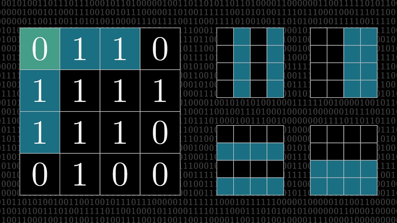
But what are Hamming codes? The origin of error correction — 3Blue1Brown

3Blue1Brown

By structuring parity checks across binary grid subsets rather than duplicating entire messages, systems isolate and repair single-bit corruptions while detecting two-bit failures at a fraction of traditional redundancy cost.

AI-assisted summary of But what are Hamming codes? The origin of error correction — original source. Check the original for full context.

Source published:

Key ideas

  • Unlike naive triplication schemes that consume two-thirds of storage capacity with redundant copies, Hamming codes dramatically reduce overhead—for example, requiring only 9 redundancy bits to protect 247 payload bits in a 256-bit block. (0:03)
  • Richard Hamming pioneered the first error-correcting code in the 1940s at Bell Labs after recurring single-bit read errors repeatedly crashed his scheduled punch-card batch computations. (2:07)
  • By distributing multiple parity checks over structured subsets corresponding to powers of 2, a receiver can perform a binary search akin to '20 questions' to pinpoint and correct the coordinate of a flipped bit. (7:17)
  • An extended 16-bit Hamming code assigns position 0 as an overarching parity check, enabling systems to reliably locate and fix single-bit errors while independently flagging double-bit errors. (14:00)

Detailed notes

## Background Published on YouTube by Grant Sanderson on the channel 3Blue1Brown on September 4, 2020, this video offers a discovery-oriented introduction to error-correcting codes. The video description frames the lesson as an intuitive exploration of Richard Hamming's pioneering work, connecting viewers to an interactive web tool, a related chessboard puzzle, and Ben Eater's breadboard demonstration.

## TL;DR Rather than relying on wasteful brute-force methods like triplicating data, Hamming codes introduce a highly efficient strategy for locating and repairing corrupted bits using mathematically coordinated parity checks. By placing parity bits at indices that are powers of two, the system functions like a game of twenty questions, systematically halving the search space to isolate the row and column of any single flipped bit. Because parity bits fall within the same grid, they inherently protect themselves against noise just like message payload bits. Expanding the grid with an overarching parity bit at position zero yields an extended Hamming code that reliably fixes single-bit errors while detecting two-bit corruptions.

## Atmosphere & style The presentation carries 3Blue1Brown's hallmark meditative clarity, blending Grant Sanderson's gentle, curious narration with methodical geometric visualizations. It feels less like a dry lecture and more like an intellectual puzzle hunt, inviting viewers to actively reinvent Hamming's original thought process from scratch. The arc progresses smoothly from the practical frustration of corrupted punch cards to moments of genuine aesthetic appreciation, culminating in quiet wonder at how binary counting can turn messy data corruption into an elegant, self-healing system.

## Bulletin - [00:03](https://www.youtube.com/watch?v=X8jsijhllIA&t=3s) Unlike naive triplication schemes that consume two-thirds of storage capacity with redundant copies, Hamming codes dramatically reduce overhead—for example, requiring only 9 redundancy bits to protect 247 payload bits in a 256-bit block. - [02:07](https://www.youtube.com/watch?v=X8jsijhllIA&t=127s) Richard Hamming pioneered the first error-correcting code in the 1940s at Bell Labs after recurring single-bit read errors repeatedly crashed his scheduled punch-card batch computations. - [07:17](https://www.youtube.com/watch?v=X8jsijhllIA&t=437s) By distributing multiple parity checks over structured subsets corresponding to powers of 2, a receiver can perform a binary search akin to '20 questions' to pinpoint and correct the coordinate of a flipped bit. - [14:00](https://www.youtube.com/watch?v=X8jsijhllIA&t=840s) An extended 16-bit Hamming code assigns position 0 as an overarching parity check, enabling systems to reliably locate and fix single-bit errors while independently flagging double-bit errors.

## Key takeaways - [00:03](https://www.youtube.com/watch?v=X8jsijhllIA&t=3s) Everyday digital storage formats, such as scratched CDs and DVDs, rely on error correction to reconstruct perturbed bitstreams into bit-for-bit replicas of the original files. - [00:03](https://www.youtube.com/watch?v=X8jsijhllIA&t=3s) Naive triplication corrects errors by taking the best two out of three bits, but it incurs a prohibitive 66.7% redundancy overhead. - [02:07](https://www.youtube.com/watch?v=X8jsijhllIA&t=127s) Error-correcting codes constrain valid data transmissions to a tiny subset within the broader space of possible bit configurations, mapping corrupted patterns back to the nearest valid neighbor. - [02:07](https://www.youtube.com/watch?v=X8jsijhllIA&t=127s) Richard Hamming developed the technique at Bell Labs in the 1940s out of frustration with single-bit punch-card misreads halting his batch computations. - [04:16](https://www.youtube.com/watch?v=X8jsijhllIA&t=256s) A standard parity bit forces the total count of 1s in a block to be even, providing a simple way to detect an odd number of altered bits using a single check bit. - [07:17](https://www.youtube.com/watch?v=X8jsijhllIA&t=437s) A solitary global parity check cannot locate where an error occurred, nor can it detect an even number of bit flips. - [07:17](https://www.youtube.com/watch?v=X8jsijhllIA&t=437s) Hamming codes query targeted subsets of bit positions across the block, operating like a game of 20 questions that halves the space of suspect bit coordinates with each check. - [10:07](https://www.youtube.com/watch?v=X8jsijhllIA&t=607s) Arranging a 16-bit block into a 4x4 grid allows two parity checks to isolate the error's column and two additional parity checks to isolate its row. - [12:30](https://www.youtube.com/watch?v=X8jsijhllIA&t=750s) Because parity bits are embedded directly within the grid's power-of-two coordinates, any flip in a parity bit is self-corrected by the exact same group of checks. - [12:30](https://www.youtube.com/watch?v=X8jsijhllIA&t=750s) Hamming codes scale logarithmically: a 256-bit block requires only 8 parity bits to pinpoint any single-bit error across 248 payload bits. - [14:00](https://www.youtube.com/watch?v=X8jsijhllIA&t=840s) Discarding index 0 produces a 15-11 Hamming code, allowing an all-even check syndrome to unambiguously represent zero transmission errors. - [14:00](https://www.youtube.com/watch?v=X8jsijhllIA&t=840s) An extended Hamming code reserves index 0 to enforce parity over the entire block, allowing the system to distinguish clean data, correct single-bit flips, and detect double-bit errors. - [16:06](https://www.youtube.com/watch?v=X8jsijhllIA&t=966s) Encoding an 11-bit message requires placing data bits into non-parity indices (3, 5-7, 9-15) and sequentially computing parity bits at indices 1, 2, 4, 8, and finally index 0. - [17:48](https://www.youtube.com/watch?v=X8jsijhllIA&t=1068s) Decoding evaluates the internal subset parities to intersect the row and column of a flipped bit, while the full-block parity verifies that only a single error occurred.

## Detailed walkthrough ### [00:03](https://www.youtube.com/watch?v=X8jsijhllIA&t=3s) The Magic of Error Correction and the Problem of Redundancy

A scratched CD or DVD illustrates an everyday marvel: despite physical scratches modifying the zeros and ones read off the disc, consumer electronics can decode the perturbed signal into a flawless, bit-for-bit recreation of the original file. While digital files of every kind—video, audio, text, executable code, and images—are ultimately sequences of bits, protecting them against corruption is fundamentally a question of efficiency. A naive strategy would be simple triplication: store three identical copies of every single bit, examine them on playback, and take the best two out of three whenever an inconsistency appears. However, this brute-force method forces two-thirds of all available capacity to be consumed by pure redundancy, and it still fails to offer strong guarantees if multiple bit flips strike the same group.

```mermaid flowchart TD accTitle: Trade-off between naive repetition and Hamming error correction accDescr: Contrasts triplication yielding 66 percent overhead against a 256-bit Hamming block using only 9 redundancy bits.

subgraph Naive["Naive 3x Repetition"] N1["1 Data Bit"] --> N2["Store 3 Copies"] N2 --> N3["Overhead: 66.7% Redundancy"] end

subgraph Hamming["Hamming Approach"] H1["247 Data Bits"] --> H2["Combine with 9 Parity Bits"] H2 --> H3["Total: 256-Bit Block<br/>Overhead: ~3.5%"] H3 --> H4["Fixes any 1 bit flip<br/>Detects any 2 bit flips"] end ```

The mathematical problem is how to guarantee error correction while surrendering as little capacity as possible. For instance, in a 256-bit block constructed with the method presented here, only 9 bits need to act as redundancy, leaving 247 bits entirely open for substantive data. From just this single block alone, an automated system can determine whether a bit flipped and isolate its exact coordinate to restore it.

- Triplication consumes $66.\overline{6}\%$ of total storage space for redundancy. - A 256-bit block under this scheme requires only 9 redundancy bits, leaving 247 bits for payload. - Single-bit flips can be both located and corrected; two-bit flips can be reliably detected as errors, even though the receiver cannot resolve where they occurred. - As the speaker reflects on the ability to pinpoint an error from an isolated block: “And honestly, that feels like magic.”

---

[02:07](https://www.youtube.com/watch?v=X8jsijhllIA&t=127s) Richard Hamming and the Principles of Error-Correcting Codes

Error-correcting codes have spent the better part of the last century supplying deep mathematical ideas to real-world hardware. While modern applications often lean toward more sophisticated schemes such as Reed-Solomon algorithms, Hamming codes provide an exceptionally intuitive introduction to the discipline. Conceptually, all error correction rests on restricting valid transmissions to a small subset within the expansive space of all possible bit arrangements. In the same way human readers spot a typographical error in an incorrectly spelled word and intuitively map it to the nearest valid word in a dictionary, an error-correcting receiver maps an invalid received pattern back to the closest permissible neighbor.

The historical origin traces back to the 1940s at Bell Labs. A young Richard Hamming was allocated precious, limited runtime on a large, costly punch-card computer. His batch-processing jobs routinely crashed when single bits were misread from the cards. As the speaker highlights this turning point: “Frustration being the crucible of invention, he got so fed up that he invented the world's first error correction code.” Rather than explaining the technique purely by rote, the conceptual roadmap is aimed at guiding learners to actively reinvent the mechanism themselves, mirroring the hardware implementation featured in Ben Eater's breadboard demonstration.

---

[04:16](https://www.youtube.com/watch?v=X8jsijhllIA&t=256s) Setting Up the 16-Bit Block and the Parity Check

To explore Hamming's logic, consider a 16-bit block whose positions are indexed from 0 through 15. Instead of clustering redundant bits together at the end of the block, four specific positions are earmarked for redundancy, placed squarely at indices that are powers of 2. Although this technically leaves 11 bits of actual payload due to a minor nuance at position 0, these four bits do not blindly clone data; they act as a coordinated system of checks managed by a "sender" and verified by a "receiver" (which equally models reading data across time from storage).

```mermaid flowchart LR accTitle: The 16-bit grid indexing and role assignment accDescr: Displays a 4x4 matrix indexed from 0 to 15, distinguishing parity bit indices from data indices.

subgraph Grid["16-Bit Block Indexing (Positions 0-15)"] direction TB subgraph Row0["Row 0"] P0["0 (Special)"] --- P1["1 (Parity: 2^0)"] --- P2["2 (Parity: 2^1)"] --- D3["3 (Data)"] end subgraph Row1["Row 1"] P4["4 (Parity: 2^2)"] --- D5["5 (Data)"] --- D6["6 (Data)"] --- D7["7 (Data)"] end subgraph Row2["Row 2"] P8["8 (Parity: 2^3)"] --- D9["9 (Data)"] --- D10["10 (Data)"] --- D11["11 (Data)"] end subgraph Row3["Row 3"] D12["12 (Data)"] --- D13["13 (Data)"] --- D14["14 (Data)"] --- D15["15 (Data)"] end end ```

The bedrock of this system is the classic single-bit parity check. In a standard parity check, a sender reserves a single bit to constrain the entire block so that the total count of 1s across the message is an even number. If the count of 1s in the data starts out odd (such as 7), the parity bit is flipped to 1 to force the total sum to be even; if the count is already even, the parity bit remains 0. Parity can thus be represented numerically as 0 (even) or 1 (odd).

- Bit positions run from index 0 to 15. - Parity bit positions are allocated at powers of 2 ($1, 2, 4, 8$). - Position 0 serves a nuanced auxiliary role, yielding an 11-bit user data capacity out of 16 total bits. - Flipping any single bit inevitably shifts the total sum from even to odd (or vice versa), allowing immediate detection of an odd number of faults. - As the speaker notes regarding this mechanism: “This is pretty simple, deceptively simple, but it's an incredibly elegant way to distill the idea of change anywhere in a message to be reflected in a single bit of information.”

---

[07:17](https://www.youtube.com/watch?v=X8jsijhllIA&t=437s) Limitations of Parity and the "20 Questions" Subsets

A solitary parity bit suffers from severe limitations: an even number of errors (such as two flipped bits) cancels out the parity shift, masquerading as a perfectly valid, error-free block. Furthermore, an odd parity reveals only that an error exists somewhere in the block, without giving any indication of its location. Because intense random noise can always theoretically transform one legitimate block into another, no error control scheme can offer absolute certainty; the practical goal is bounding vulnerability within a threshold of bit flips.

```mermaid flowchart TD accTitle: Hamming parity subset strategy accDescr: Shows how multiple targeted parity queries narrow down the position of an error like twenty questions.

E["Single Bit Error Occurs"] --> Q1{"Parity Check 1<br/>Odd positions: 1, 3, 5, 7, 9, 11, 13, 15<br/>Parity bit: Index 1"} Q1 -->|"Parity Fails (Odd)"| O["Error is in an ODD position"] Q1 -->|"Parity Passes (Even)"| EV["Error is in an EVEN position (or no error)"]

O --> Q2{"Parity Check 2<br/>Right-hand columns: 2, 3, 6, 7, 10, 11, 14, 15<br/>Parity bit: Index 2"} EV --> Q2

Q2 -->|"Combined Checks"| LOC["Successive queries chop space of possibilities in half"] ```

Hamming's breakthrough was to avoid applying parity globally to the whole block, instead distributing separate parity checks across specifically structured subsets of the bits. This operates like a game of 20 questions, where each parity query asks a binary yes/no question that halves the search space.

- **Check 1 (Odd Indices):** Covers positions 1, 3, 5, 7, 9, 11, 13, and 15, using position 1 as its governing parity bit. If this group tests odd, the receiver knows the error lies within an odd index; if even, it lies among the even indices (or no error occurred). - **Check 2 (Right Half of Grid):** Covers indices located on the right half of the 4x4 representation (positions 2, 3, 6, 7, 10, 11, 14, and 15), regulated by position 2. If its parity is already even, the sender leaves bit 2 at 0. - As the speaker describes the search strategy: “The overall feeling is a bit like playing a game of 20 questions, asking yes or no queries that chop the space of possibilities in half.”

[10:07](https://www.youtube.com/watch?v=X8jsijhllIA&t=607s) Pinpointing the Column and Row with Parity Checks

On the receiving end of a transmission, checking the parity of the right half of the four-by-four grid immediately establishes whether an error exists among those eight bits. If that group evaluates to odd, the receiver knows an error occurred somewhere on the right; if even, either no error occurred or it sits on the left half. For the moment, the scheme assumes at most one single-bit error across the entire block, as multiple errors cause this basic premise to break down completely. Combining this check with the first test—which tests the odd columns—allows the receiver to isolate the exact column of the error. If an error is detected in both the odd columns and the right half, the error must lie in the final column; an error in the right half without an odd-column error points to the second-to-last column; an odd-column error without a right-half error points to the second column; and if neither check flags anything, any potential error is confined to the leftmost column (or there is no error at all). As Grant Sanderson notes: “Which is all a rather belabored way to say that two parity checks let us pin down the column.”

```mermaid flowchart TD accTitle: Two-Dimensional Parity Check Isolation accDescr: Flowchart showing how four parity checks combine to determine the exact column and row of a single-bit error. subgraph ColGroup["Column Detection"] C1["Odd Columns Check<br>(Bit 1)"] C2["Right-Half Check<br>(Bit 2)"] ColOut["Target Column Identified"] C1 --> ColOut C2 --> ColOut end

subgraph RowGroup["Row Detection"] R1["Odd Rows Check<br>(Bit 4)"] R2["Bottom-Half Check<br>(Bit 8)"] RowOut["Target Row Identified"] R1 --> RowOut R2 --> RowOut end

ColOut --> Intersect["Target Position (Row, Column)"] RowOut --> Intersect ```

Following the exact same logic, the sender and receiver use two additional parity checks to isolate the row. Position 4 serves as the parity bit to enforce even parity across the odd rows, while position 8 acts as the parity bit across the bottom two rows. If an error occurs during transmission at position 3, it flips the parity of the odd-column group and the right-half group, immediately signaling to the receiver that the error is in the rightmost column. However, position 3 leaves the odd-row check and the bottom-half check completely unaffected, pinning the error to the top row. The intersection of that row and column uniquely identifies bit 3, allowing the receiver to flip it back and correct the data. This reveals an underlying connection between the four questions and binary counting.

[12:30](https://www.youtube.com/watch?v=X8jsijhllIA&t=750s) Self-Correcting Parity Bits and Scaling Efficiency

A common concern is what happens if noise flips one of the error-correcting parity bits themselves rather than a message bit. Because parity bits are included in the grid just like any other bit, the four parity questions automatically track down a flipped parity bit in the exact same manner. While the primary goal is solely to safeguard the payload bits—with the parity bits simply along for the ride—protecting the parity bits emerges naturally as a structural byproduct of the layout. Grant Sanderson emphasizes this symmetry: “Take a moment to think about how any error among these four special bits is going to be tracked down just like any other, with the same group of four questions.”

The true power of this scheme lies in how efficiently it scales: - In a 256-bit block, locating any specific bit requires only eight yes-or-no questions, effectively performing a binary search down to an individual coordinate. - Implementing those eight questions requires sacrificing only eight bits out of the 256 to serve as parity bits. - The remaining 248 bits are entirely free to carry arbitrary message data, achieving a high data-to-overhead ratio. - Rather than redundantly duplicating the entire transmission, the parity bits are smartly determined by mathematical subsets, achieving robust single-error correction at minimal cost.

[14:00](https://www.youtube.com/watch?v=X8jsijhllIA&t=840s) The 15-11 Code and the Extended Hamming Code

A subtle edge case arises when all four parity checks evaluate to even. Under four yes-or-no tests, exactly $2^4 = 16$ distinct outcomes are possible, which neatly matches the 16 positions in a four-by-four grid. However, the system also needs to represent a seventeenth outcome: the condition where no error has occurred. If all four checks pass as even, the receiver cannot distinguish between a clean transmission and a bit flip located at position 0. The most straightforward workaround is simply discarding index 0 entirely. Working with a 15-bit block gives 11 message bits and 4 parity bits, producing what is standardly known as a 15-11 Hamming code, where an all-even test unambiguously means zero errors.

```mermaid flowchart TD accTitle: Extended Hamming Code Error Classification accDescr: Decision logic using four internal parity checks alongside the overall zeroth parity bit to separate zero errors, single-bit errors, and two-bit errors. Checks{"Four Parity Checks<br>Detect Error?"} Overall{"Overall Bit 0<br>Parity Odd?"}

Checks -->|"No (All Even)"| O1{"Overall Bit 0<br>Parity Odd?"} O1 -->|"No (Even)"| NoErr["No Errors Detected"] O1 -->|"Yes (Odd)"| P0Err["Single Error at Bit 0"]

Checks -->|"Yes (Non-zero syndrome)"| Overall Overall -->|"Yes (Odd)"| SingleErr["Single-Bit Error<br>(Locate & Correct)"] Overall -->|"No (Even)"| DoubleErr["Two-Bit Error Detected<br>(Cannot Correct)"] ```

Instead of discarding position 0, an extended Hamming code puts that bit to work as an overarching parity bit that covers the entire 16-bit block: - After computing and setting the four internal error-correcting bits (at powers of 2), bit 0 is set so the total count of 1s in the entire 16-bit block is even. - If a single-bit error strikes anywhere in the block, the overall parity toggles to odd, and the internal four checks pinpoint the exact bit to fix. - If two bits flip, the overall block parity toggles twice, returning to an even state; however, the four internal checks will still flag an error condition. - Seeing an even overall block parity accompanied by non-zero flags in the internal parity checks informs the receiver that at least two errors occurred, allowing two-bit error detection even though two-bit errors cannot be corrected. Reflecting on this dual-purpose design, Sanderson remarks: “Isn't that clever?”

[16:06](https://www.youtube.com/watch?v=X8jsijhllIA&t=966s) Walkthrough: Encoding an 11-Bit Message

To prepare a message for transmission or storage, the raw data stream is first split into 11-bit chunks, with each chunk mapped into a 16-bit block. Positions corresponding to index 0 and powers of 2 (indices 1, 2, 4, and 8) are set aside for redundancy, leaving indices 3, 5, 6, 7, 9, 10, 11, 12, 13, 14, and 15 to hold the 11 message bits. Grant Sanderson directs viewers through the manual construction: “Remember, position 0 along with the other powers of 2 are reserved for error correction duty, so you start by placing the message bits in all of the remaining spots, in order.”

The sender then computes each parity bit sequentially: - Group 1 (odd columns, governed by bit 1): The message bits in this subset already exhibit an even parity, so parity bit 1 is set to `0`. - Group 2 (right two columns, governed by bit 2): The message bits in this subset start with an odd count of 1s, requiring bit 2 to be set to `1` to achieve even parity. - Group 3 (odd rows, governed by bit 4): The message bits here sum to an odd count, so bit 4 is set to `1`. - Group 4 (bottom two rows, governed by bit 8): The message bits in the bottom two rows also total an odd parity, meaning bit 8 is set to `1`. - Overall parity bit (position 0): With the four internal parity bits assigned, the parity of all bits across the full 16-bit block is checked. Because the entire block already has an even parity, bit 0 is set to `0`. Once dispatched, the overarching block and all four constituent subsets evaluate to an even parity of `0`.

[17:48](https://www.youtube.com/watch?v=X8jsijhllIA&t=1068s) Walkthrough: Receiving, Correcting, and the Python Teaser

Simulating the receiver's perspective illustrates how decoding operates blind to the original contents. Upon receiving an altered block where one or two bits may have flipped, the receiver evaluates each parity rule in sequence: - Parity check 1 evaluates to even, indicating that any error must be restricted to the even columns. - Parity check 2 evaluates to odd, proving an error exists and narrowing the column down to the third column. - Parity check 3 evaluates to even, eliminating the odd rows from suspicion. - Parity check 4 evaluates to odd, establishing that the error resides in the bottom half.

Matching the intersection of the third column and the bottom rows isolates the fault precisely to position 10. Evaluating the overarching parity across all 16 bits yields an odd count, verifying that exactly one flip occurred rather than two. As Sanderson cautions regarding multi-bit limitations: “If it's three or more, all bets are off.” After flipping bit 10 back to its correct state, extracting the 11 payload bits completely restores the sender's original message. The core logic of this entire error-locating sequence can be condensed into a single line of Python, an elegant unified operation explored in part 2.

## Mentioned Richard Hamming, Bell Labs, Reed-Solomon, Ben Eater, Matt Parker, Harry Li, Vincent Rubinetti, The Art of Doing Science and Engineering, Python, Manim

## Video description A discovery-oriented introduction to error correction codes. Part 2: https://youtu.be/b3NxrZOu_CE Ben Eater:'s take: https://youtu.be/h0jloehRKas Help fund future projects: https://www.patreon.com/3blue1brown An equally valuable form of support is to simply share some of the videos. Special thanks to these supporters: https://3b1b.co/hamming-thanks

Heavily related is the chessboard puzzle I did with Matt Parker: https://youtu.be/as7Gkm7Y7h4

You can read Hamming's own perspective on his discovery of these codes in chapter 12 of "The Art of Doing Science and Engineering". https://amzn.to/3lwcnmh

The viewer Harry Li made an interactive on this topic: https://harryli0088.github.io/hamming-code/

Thanks to these viewers for their contributions to translations Hebrew: Omer Tuchfeld Hungarian: Fabó Bence Spanish: agustin-j

------------------

These animations are largely made using manim, a scrappy open-source python library: https://github.com/3b1b/manim

If you want to check it out, I feel compelled to warn you that it's not the most well-documented tool, and it has many other quirks you might expect in a library someone wrote with only their own use in mind.

Music by Vincent Rubinetti. Download the music on Bandcamp: https://vincerubinetti.bandcamp.com/album/the-music-of-3blue1brown

Stream the music on Spotify: https://open.spotify.com/album/1dVyjwS8FBqXhRunaG5W5u

------------------

3blue1brown is a channel about animating math, in all senses of the word animate. And you know the drill with YouTube, if you want to stay posted on new videos, subscribe: http://3b1b.co/subscribe

Various social media links: Website: https://www.3blue1brown.com Twitter: https://twitter.com/3blue1brown Reddit: https://www.reddit.com/r/3blue1brown Instagram: https://www.instagram.com/3blue1brown_animations/ Patreon: https://patreon.com/3blue1brown Facebook: https://www.facebook.com/3blue1brown

[Source](https://www.youtube.com/watch?v=X8jsijhllIA)

中文简报

汉明码纠正比特翻转以大幅降低数字存储开销 通过在二进制网格子集间构建奇偶校验而非复制完整信息,系统能够以传统冗余成本的一小部分隔离并修复单比特损坏,同时检测双比特故障。 汉明码没有依赖将数据复制三份等浪费资源的蛮力方法,而是引入了一种高效策略,利用数学上协同的奇偶校验来定位和修复受损比特。通过将校验比特放置在2的幂次索引处,该系统运作起来类似于二十个问题的游戏,能够系统性地将搜索空间减半,从而准确定位任何单个翻转比特的行和列。由于校验比特位于同一网格内,它们与信息有效载荷比特一样,天然受到保护以抵御噪声。在位置0添加一个全局校验比特来扩展网格,便可形成扩展汉明码,该编码能可靠地修复单比特错误,同时检测双比特损坏。 不同于用冗余副本消耗三分之二存储容量的简单三模冗余方案,汉明码大幅降低了开销——例如,在一个256比特的区块中,仅需9个冗余比特即可保护247个有效载荷比特。 (0:03) 20世纪40年代,理查德·汉明在贝尔实验室开创了首个纠错码,此前反复出现的单比特读取错误屡次导致他安排的打孔卡批处理计算崩溃。 (2:07) 通过在对应2的幂次的结构化子集上分布多个奇偶校验,接收方可以进行类似于“20个问题”的二分搜索,从而查明并纠正翻转比特的坐标。 (7:17) 扩展16比特汉明码将位置0指定为全局奇偶校验,使系统能够可靠地定位并修复单比特错误,同时独立标记出双比特错误。 (14:00)

Reading summary

Grant Sanderson explains how Richard Hamming's parity-based error-correcting codes replace inefficient brute-force redundancy with targeted binary queries, enabling systems to pinpoint and repair single-bit corruptions while detecting two-bit failures at minimal overhead. The Efficiency Crisis of Naive Redundancy (0:03) Digital error correction ensures corrupted signals, such as scratched optical discs, can be reconstructed into bit-for-bit replicas of their source data. While simple triplication can resolve single-bit errors through majority voting, this brute-force approach requires a punishing 66.7% capacity overhead and breaks down when multiple bit flips strike the same group. Richard Hamming formulated the first error-correcting code in the 1940s at Bell Labs after recurring bit-read errors repeatedly crashed his punch-card batch computations. Binary Subset Checks Pinpoint Error Coordinates (7:17) A classic parity bit forces the sum of ones across a block to be even, enabling the detection of an odd count of flipped bits, but it cannot reveal where the error occurred or catch an even number of flips. Hamming solved this by organizing blocks into structured, overlapping subsets that function like a game of 20 questions, where each parity check halves the remaining search space. Grid Intersections and Inherent Symmetry (10:07) In a 16-bit block arranged as a 4x4 grid, parity bits are stationed at indices that are powers of two (1, 2, 4, and 8). Parity checks on odd columns (bit 1) and right-hand columns (bit 2) isolate the faulty column, while checks on odd rows (bit 4) and bottom rows (bit 8) identify the row. Their intersection exposes the exact corrupted coordinate, such as bit 3 or bit 10, allowing the receiver to flip it back. Because the parity bits are embedded directly within the grid structure, an error landing on a parity bit is located and resolved by the exact same mechanism. Extended Codes and Logarithmic Scaling (14:00) Because four binary checks produce only 16 outcomes, an all-even result cannot distinguish between zero errors and a flip at index 0. Standard 15-11 Hamming codes drop index 0 entirely, leaving 11 payload bits and 4 parity bits. Alternatively, extended Hamming codes use position 0 as an overarching parity check covering all 16 bits. If the internal checks flag an error but the overall block parity remains even, the receiver detects a two-bit error that cannot be corrected. The scheme scales logarithmically: a 256-bit block requires only 8 parity bits to pinpoint any single coordinate, leaving 248 bits for message data. Hamming codes bound vulnerability to low-order errors but fail when noise exceeds their design limits; as Sanderson cautions, three or more bit flips undermine the assumptions entirely, leaving the data corrupted without a reliable warning.

精炼阅读摘要

根据 3Blue1Brown 的梳理,错误校正的核心在于平衡冗余开销与数据可靠性;理查德·汉明(Richard Hamming)通过将奇偶校验拓展为类似“二十个问题”的子集二分查询,构建出能够以极低容量损耗精准定位并修复单比特错误的汉明码。 冗余困境与汉明纠错码的历史源流 (0:03) 划痕光盘能被无损读取展示了纠错技术的效能。在数字存储与传输中,最朴素的容错策略是将每个比特复制三份并采用多数表决法,但这会导致 66.7% 的存储空间沦为纯冗余,且同组发生多处翻转时依然失效。数学上的核心诉求是如何以最小的容量代价获得确定的纠错能力。20 世纪 40 年代,贝尔实验室的理查德·汉明因打孔卡计算机频繁误读单比特导致程序崩溃,促使他发明了世界上首个纠错码。 纠错码的基本原理是将合法的传输模式限制在所有可能比特排列的一个微小子集内。正如人类读者遇到拼写错误的单词时能直观对应到词典中最接近的词汇一样,接收端也会将受噪声干扰的非法数据模式映射回距离最近的合法代码。尽管现代工程常采用更复杂的里德-所罗门(Reed-Solomon)等算法,汉明码仍是理解纠错理论最直观的基石。 子集划分与二十个问题的网格定位 (7:17) 传统单比特奇偶校验只能通过强制让“1”的总数为偶数来发现奇数个翻转,既无法得知错误位置,面对双比特翻转时更会彻底失效。汉明的关键突破在于不再对全局笼统施加单一校验,而是将校验位分散并覆盖至经过专门设计的比特子集,其逻辑如同通过“二十个问题”游戏的二元是非问答不断将嫌疑范围减半。 在一个 16 比特构成的四乘四网格中,校验位被安置在 2 的幂次方索引处(1、2、4、8)。位置 1 校验所有奇数列,位置 2 校验右半区两列,两者结合即可将发生翻转的列坐标唯一锁定;位置 4 负责奇数行校验,位置 8 负责下半区两行校验,两者结合便锁定了行坐标。行列相交的位置即为出错比特。值得注意的是,校验位自身也完全落在该检测框架内,若校验位本身发生翻转,同样会被这套问题自动定位并复原。 扩展汉明码与双比特错误检测机制 (14:00) 由四个校验问题构成的系统最多能产生 16 种不同的是非组合,恰好对应四乘四网格的 16 个坐标。然而,系统还需要额外表示“无错误发生”这第 17 种状态;如果所有校验均表现为偶数,接收端无法区分究竟是传输完全正常,还是索引 0 发生了翻转。一种折中方式是直接废弃索引 0,构建包含 11 个数据位与 4 个校验位的标准 15-11 汉明码;而扩展汉明码则将位置 0 设为覆盖整个 16 比特数据块的全局校验位。 在扩展汉明码中,位置 0 强制使全部 16 比特的“1”总数为偶数。若块内发生单比特错误,全局校验必然变为奇数,此时借助内部四个校验即可精确定位并纠正该错误;若发生双比特翻转,全局校验翻转两次后依旧保持为偶数,但内部校验仍会报告异常。接收端一旦观察到“全局为偶但内部报错”,便能判定出现了双比特错误,从而实现了单错误纠正与双错误检测(SECDED)的兼顾。 编码解码实操与规模化扩展效率 (16:06) 在 16 比特扩展汉明码的实际编码中,11 比特有效载荷按顺序填入除 0 和 2 的幂次方以外的可用索引(3、5、6、7、9、10、11、12、13、14、15)。发送端依次计算第 1、2、4、8 位的奇偶值以满足各子集偶校验,最后设定位置 0 使整块总和为偶。接收端解码时独立执行各项校验:例如当第 2 项与第 4 项校验报错,便分别锁定第三列与下半区,交叉得出位置 10 发生错误;此时若全局校验为奇数,即可判定仅有单比特出错,翻转位置 10 即可完整还原原本的 11 比特数据。 该编码方案在规模扩大时表现出极高的效率。若扩展至 256 比特的数据块,定位单一坐标仅需 8 次二分询问(即 8 个校验位),加上位置 0 的全局校验总共仅需 9 个冗余位,剩余 247 比特全部可用作实际数据载荷,冗余开销骤降至约 3.5%,远优于简单复制备份的低效模式。 主讲人格兰特·桑德森强调,若数据块遭遇 3 个或更多比特翻转,该校验体系将彻底失效并失去保障。汉明码的核心定位过程在底层能被高度浓缩为单行 Python 代码,其展现出的数学结构确立了数字容错通信的重要范式。

Detailed notes — zh

## Background 该视频由知名数学科普频道 3Blue1Brown 于 2020 年 9 月 4 日发布在 YouTube 上。视频简介将其描述为一次面向发现之旅的纠错码入门介绍,追溯了理查德·汉明在贝尔实验室因打孔卡读取错误而发明汉明码的起源故事,并关联了相关的棋盘谜题与互动教学资源。 ## TL;DR 视频从划痕光盘仍能播放的现象切入,对比了开销巨大的朴素三重冗余与极其精简高效的汉明码。主讲人以 16 比特网格为例,生动拆解了如何将奇偶校验转化为类似“二十个问题”的二分搜索策略,通过 4 个位于 2 的幂次方的校验位精准定位出错的行列坐标。视频进一步介绍了舍弃第 0 位的标准 15-11 汉明码,以及将第 0 位重新作为全局校验从而实现双比特错误检测的扩展汉明码,并以完整的端到端实战演练展示了编码与解码的精妙闭环。 ## Atmosphere & style 视频展现了 3Blue1Brown 标志性的从容、典雅与启发式叙事风格。主讲人 Grant Sanderson 语气温和沉稳,借助流畅直观的动画逐步揭开复杂的数学结构,引导观众在被剧透前主动暂停思考。整期内容充满了对数学对称性与信息论巧思的纯粹赞叹,让严谨的计算机底层通信理论如同精彩的侦探解谜般引人入胜。 ## Bulletin - [00:03](https://www.youtube.com/watch?v=X8jsijhllIA&t=3s) 朴素的三重冗余方案需付出约 66.7% 的存储空间开销且多比特错误时易失效,而汉明纠错码可在 256 比特块中仅用 9 个校验比特保护 247 个数据比特,将冗余率大幅降至约 3.5%。 - [08:27](https://www.youtube.com/watch?v=X8jsijhllIA&t=507s) 汉明码的本质是将单比特奇偶校验拆解为类似“二十个问题”的二分询问,通过在 2 的幂次方位置设置交叠子集校验位,实现以对数级开销精准定位错误坐标。 - [14:59](https://www.youtube.com/watch?v=X8jsijhllIA&t=899s) 在 16 比特结构中引入位置 0 作为全块奇偶校验位构建扩展汉明码,可在保持单比特错误纠正能力的同时,可靠检出双比特翻转错误。 ## Key takeaways - [00:03](https://www.youtube.com/watch?v=X8jsijhllIA&t=3s) 数字纠错技术通过在数据中引入数学冗余,使得划伤的光盘或嘈杂信道中的数据能够实现逐比特无损还原。 - [02:07](https://www.youtube.com/watch?v=X8jsijhllIA&t=127s) 纠错的基本数学原理是在庞大的消息空间中定义少量的合法码字,并在受到噪声破坏时将非法状态映射至最近的有效邻居。 - [02:07](https://www.youtube.com/watch?v=X8jsijhllIA&t=127s) 理查德·汉明在 20 世纪 40 年代因贝尔实验室打孔卡计算机频繁因单比特误读崩溃退出,从而被激发发明了世界上首个纠错码。 - [04:16](https://www.youtube.com/watch?v=X8jsijhllIA&t=256s) 传统奇偶校验通过让数据块中 1 的总数保持为偶数来敏锐察觉单比特翻转,但其完全无法提供错误发生的位置信息,且对偶数个翻转存在盲区。 - [08:27](https://www.youtube.com/watch?v=X8jsijhllIA&t=507s) 汉明将奇偶校验应用到精心挑选的重叠子集上,使每一次校验结果都如同二分搜索的是非回答,逐步收窄单比特错误的坐标范围。 - [10:07](https://www.youtube.com/watch?v=X8jsijhllIA&t=607s) 通过对奇数列和右半部分进行两次奇偶校验求交集,接收端即可无歧义地精确定位错误落在方阵的哪一列。 - [11:11](https://www.youtube.com/watch?v=X8jsijhllIA&t=671s) 通过位置 4(监控奇数行)和位置 8(监控下半区)的两次行校验,系统能够锁定行坐标,并与列定位结合直接定位到具体单元格。 - [11:11](https://www.youtube.com/watch?v=X8jsijhllIA&t=671s) 汉明码方案天然具备自检性,冗余校验位自身如果发生翻转,同样会被这套二分搜索校验网络准确锁定并纠正。 - [12:59](https://www.youtube.com/watch?v=X8jsijhllIA&t=779s) 标准的 15-11 汉明码舍弃了歧义的位置 0,利用 4 个校验位保护 11 个数据比特,全偶状态清晰地对应无错误发生。 - [14:59](https://www.youtube.com/watch?v=X8jsijhllIA&t=899s) 通过将位置 0 重新启用为覆盖整块的全局校验位,扩展汉明码在检测到“全局偶数、局部非零”时能准确识别出双比特错误。 - [12:59](https://www.youtube.com/watch?v=X8jsijhllIA&t=779s) 汉明码的校验位数量仅随数据块尺寸呈对数级增长,在 256 比特块中仅需 8 个校验位即可完成单比特错误定位,展示了极高的信息效率。 - [16:06](https://www.youtube.com/watch?v=X8jsijhllIA&t=966s) 整套看似繁琐的手工网格行列校验推导,在底层与二进制计数深度绑定,并可浓缩为单一算子与单行 Python 核心代码实现。 ## Detailed walkthrough ### [00:03](https://www.youtube.com/watch?v=X8jsijhllIA&t=3s) 纠错码的魔力与冗余的代价 当你划伤一张光盘(CD 或 DVD)时,它往往仍能流畅播放其中的影音内容。从物理上看,划痕确实破坏了光盘表面的二进制数据,读取设备读出的 0 和 1 与最初写入的内容并不一致。然而只要划痕没有严重到彻底损毁,解码系统就能通过数学算法,从错误的数据中精确还原出最初编码的原始文件,实现逐比特(bit-for-bit)的无损复原。无论是存储数据还是在嘈杂信道中传输数据,这种抗噪特性的背后都凝聚着一整套绝妙的数学构想。 其实,想出一种抵御错误的方法并不需要高深的技术。任何数字文件本质上都是一串 0 和 1 的序列。最简单粗暴的策略是“三重冗余”:为每一个比特连续存储三份拷贝。读取端在遇到歧义时只需采用“三局两胜”(少数服从多数)的表决原则,就能纠正任意单比特翻转。但这种方法的代价极其高昂,有整整三分之二(约 66.7%)的存储空间被纯粹的重复数据白白浪费,而且一旦同时翻转了两个比特,这种简单的表决策略就会彻底失效。 真正迷人且具有实际价值的挑战在于:如何在牺牲尽可能少存储空间的前提下,实现精准的错误纠正。以汉明码(Hamming code)为例,如果将数据按 256 比特的区块进行组织,只需要拿出区区 9 个比特作为冗余校验,剩下的 247 个比特都可以全部用于装载真正的信息数据。令人惊叹的是,在这个 256 比特的区块中,只要有任意一个比特发生翻转,机器仅凭观察这一个区块,就能确切知道发生了错误,并分毫不差地定位出翻转发生在哪个位置,从而将其纠正。这种四两拨千斤的效果展现了数学的极致魅力;对于这个特定的编码体系,即使有两处比特同时翻转,机器也至少能明确探测出“存在两个错误”,即便此时它无法直接修复。 ```mermaid flowchart TD accTitle: 数据纠错方案效率对比 accDescr: 对比朴素三重冗余与汉明码在冗余开销和纠错能力上的差异 subgraph Naive["方案 A:三重冗余 (Naive Triplication)"] direction TB N1["输入比特:1"] --> N2["编码:1 1 1\n(冗余开销占 66.7%)"] N2 --> N3["多数表决解码:纠正 1 比特翻转\n多比特错误时崩溃"] end subgraph Hamming["方案 B:汉明纠错码 (Hamming Code)"] direction TB H1["输入数据:247 比特"] --> H2["加入 9 比特校验位\n(总共 256 比特,冗余开销仅 3.5%)"] H2 --> H3["精准定位并纠错 1 比特\n同时可侦测 2 比特错误"] end ``` - 三重冗余机制需要牺牲 66.7% 的存储空间,却无法对多于 1 位的翻转提供稳健保证。 - 采用汉明码机制的 256 比特区块,仅需 9 个校验比特即可覆盖 247 个数据比特(冗余率仅约 3.5%)。 ### [02:07](https://www.youtube.com/watch?v=X8jsijhllIA&t=127s) 理查德·汉明的困境与纠错原理 这类能发现并修复错误的技术被称为“纠错码”(Error Correction Codes)。在过去大半个世纪里,它催生了大量深刻的数学成果,并广泛应用于现代设备中。虽然现代工程中更多使用更为强大的高级算法(例如里德-所罗门码,即 Reed-Solomon 码),但汉明码作为该领域的鼻祖,以其构思的纯粹和精妙至今仍是不可替代的教学范本。 纠错的基本原则其实并不复杂:在所有可能构成的消息空间中,只有一部分特定的组合被定义为“有效消息”(Valid messages)。这就像人类语言中的拼写规则,正确的单词只是所有字母排列中的一小部分子集。一旦传输或存储中的某个有效消息受到噪声干扰发生畸变,接收端的任务就是将接收到的非法状态“归位”到距离它最近的有效消息邻居上,就像拼写检查器修正错别字一样。 汉明码的诞生源于 20 世纪 40 年代贝尔实验室(Bell Labs)的一段轶事。当时年轻的理查德·汉明(Richard Hamming)需要排队使用一台庞大且昂贵的打孔卡计算机。由于分配到的机时有限,他常常在周末提交批处理作业,可机器经常因为某张打孔卡上的一个比特读取错误而全盘崩溃退出。多次心血付诸东流的挫折感最终逼得汉明下定决心自行解决这个问题。正如讲述者所说:“Frustration being the crucible of invention, he got so fed up that he invented the world's first error correction code.”(挫折成了发明的熔炉,他实在受够了,于是发明了世界上第一个纠错码。) - 纠错本质上是将损坏的数据映射回消息空间中与之最近的“合法码字”。 - 贝尔实验室昂贵庞大的打孔卡机器频繁因单比特误读而停机,直接促成了汉明对自动化纠错机制的研究。 ### [04:16](https://www.youtube.com/watch?v=X8jsijhllIA&t=256s) 16 比特结构与奇偶校验基石 为了让原理清晰易懂,我们以一个 16 比特的块为例。将这 16 个比特的位置从 0 到 15 依序编号。在最初的设计设定中,实际承载有效数据的有效载荷占用了其中的 11 到 12 位,而专门划出的 4 个位置则作为冗余校验位。这里的“冗余”并不是做简单的备份,4 个比特的容量根本无法承载整个消息的复本;它们的作用是通过某种精密的数学交织,在不引入额外信息的前提下为系统赋予极高的抗错弹性。 不同寻常的是,这 4 个特殊的冗余位并没有集中打包堆放在区块的尾部,而是特意被安排在所有编号为“2 的幂次方”的位置上(即 1, 2, 4, 8,以及位置 0 处带有的特殊性质)。这种分布为后续整个机制的数学自洽埋下了伏笔,也暗示了该方案如何轻松扩展到更大的数据块(如 32、64、128 或 256 比特)。在通信模型中,处理流程包含两方:一方是负责设置这些特殊校验位的“发送方”,另一方则是负责运行检验并执行纠偏的“接收方”。需要注意,“发送”与“接收”只是抽象概念,将数据写入磁盘存储,本质上就是把一条信息从“过去”发送给“未来”。 要理解汉明码的运转,必须先掌握当时汉明头脑中已经非常成熟的基础工具——“奇偶校验”(Parity Check)。纯粹的奇偶校验只能用于检测单比特错误的存在,却完全无法指出错误发生在何处。在普通的奇偶校验中,整组比特中只留出 1 个特殊的校验位由发送方控制,其余位均用于存放常规数据。这个校验位唯一的使命,就是确保整个块内“1”的总数永远保持为偶数。如果数据中 1 的个数已经是偶数,该校验位就置为 0;如果 1 的个数是奇数,校验位就必须翻转为 1,从而强行将总数凑成偶数。 ```mermaid flowchart LR accTitle: 单比特奇偶校验工作机制 accDescr: 说明发送方如何通过设置校验位保证 1 的数量为偶数,以及单比特翻转如何触发奇偶性变化 subgraph Sender["发送端设置奇偶位"] direction TB S1["原始数据包含 7 个 '1'\n(总和为奇数)"] --> S2["将校验位设定为 1"] S2 --> S3["传输消息包含 8 个 '1'\n(总和变为偶数)"] end subgraph Channel["信道传输扰动"] direction TB S3 -->|"发生 1 比特翻转"| C1["消息中 '1' 的总数\n由偶数变为奇数"] end subgraph Receiver["接收端校验判定"] direction TB C1 --> R1{"检测 '1' 的总数奇偶性"} R1 -->|"计数为奇数"| R2["断定必然发生错误\n(但无法得知错在哪里)"] end ``` - 块中 1 的数量是偶数还是奇数被称为该集合的“奇偶性”(Parity),在数学上通常直接用 0(偶)或 1(奇)来表示。 - 奇偶校验具有极端敏锐的联动效应:整个块中任意单个比特发生变化(0 变 1 或 1 变 0),1 的总数奇偶性必然从偶数颠倒为奇数。 - 奇偶校验的缺陷在于盲区:如果发生 2 处(或任意偶数处)翻转,1 的总数依然保持偶数,系统便无法察觉。没有一种纠错机制能对抗无限的随机噪声,其核心目标始终是在既定错误上限内尽可能降低误判率。 ### [08:27](https://www.youtube.com/watch?v=X8jsijhllIA&t=507s) 子集划分与“二十个问题”寻错法 单比特奇偶校验虽然简单脆弱,但它实现了一种不可思议的信息浓缩:将整个庞大序列中“是否发生了变动”这一全局状态,精确凝练成了一个单独的二进制位。汉明最关键的直觉突破正是在这里迸发的:如果奇偶校验不再笼统地应用于整个数据块,而是分别作用于若干组精心挑选的子集上,我们就能像玩“二十个问题”(20 Questions)游戏那样,通过一连串“是或否”的二分查询,逐步将单比特错误的位置锁定在某一个具体坐标上。 把整个 16 比特网格切分成不同的重叠子集,便能让各组校验位分别反映不同维度的坐标信息。例如,我们可以设计第一个奇偶校验组,让它仅覆盖全部编号为奇数的位置(1, 3, 5, 7, 9, 11, 13, 15,共 8 个比特)。 - 如果这 8 个比特的奇偶校验报错(1 的总数为奇数),接收方立刻就能获取一条极其明确的位置信息:错误必然落在某个奇数编号上。 - 如果这 8 个比特没有报错,则意味着要么整个子集完好无损,要么错误隐藏在未被选中的偶数编号当中。 为了实现这第一项校验,必须在奇数集合中钦定一个比特来专门充当奇偶调节开关,而最合适的人选正是位置 1 本身。假如此时该 8 比特子集中 1 的总数为奇数,发送方就会把位置 1 翻转为 1,将这组子集的总数变为偶数。 紧接着是第二组奇偶校验,它选取了网格右半部分的 8 个比特(在网格布局中对应位置 2, 3, 6, 7, 10, 11, 14, 15)。这组校验则由位于位置 2 的比特专门负责调控。如果这 8 个比特当前已经包含偶数个 1,发送方就可以直接将位置 2 保持为 0 而无需改动。通过将这样多个交错分布的奇偶校验组合在一起,看似弱小的校验位便交织成了一张严密的数据侦测网。 - 汉明码的核心逻辑是将整体奇偶校验拆解为面向特定子集的多次二分询问,每一次校验都能将怀疑范围缩小一半。 - 第一个校验集(覆盖所有奇数位)由位置 1 担任校验位;第二个校验集(覆盖特定列/右半侧)由位置 2 担任校验位,二者协同开启了精确定位错误位置的可能。 ### [10:07](https://www.youtube.com/watch?v=X8jsijhllIA&t=607s) 通过两组校验精确定位列坐标 在构建 16 位方阵校验的过程中,接收端一旦检查右半部分 8 个比特组成的奇偶校验组并发现其奇偶性为奇数,就能立即断定传输错误必定潜伏在右侧这 8 个比特之中;反之,若结果为偶数,则说明要么完全没有发生错误,要么错误落在左半部分。当然,理论上可能同时出现两个错误,但此时的基线假设是在整个数据块中至多只发生一个比特错误,因为一旦错误数量超过一个,整个基础方案就会彻底崩溃。 在此基础上,将针对奇数列的前一个校验与针对右半部分的校验结合起来观察,就会展现出二分搜索的精妙威力。如果系统在奇数列和右半部分同时检测到错误,那么两者求交集,错误必定只能位于方阵的最后一列(第 3 列);如果奇数列无误但右半部分有误,则直接锁定在倒数第二列(第 2 列);如果奇数列有误而右半部分无误,则对应第二列(第 1 列);而若两项奇偶校验均未报警,便意味着错误只能在最左侧的列(第 0 列),抑或是压根没有任何错误发生。正如主讲人总结道:“Which is all a rather belabored way to say that two parity checks let us pin down the column.”(这番略显繁复的推导,说白了就是两次奇偶校验足以让我们精确定位所在的列。) ```mermaid flowchart TD accTitle: 列定位逻辑流程 accDescr: 展示如何通过奇数列检查与右半部分检查两组结果交集确定错误所在的具体列 CheckOdd{"奇数列存在错误?"} CheckRight1{"右半部分存在错误?"} CheckRight2{"右半部分存在错误?"} Col3["错误位于最后一列 (第 3 列)"] Col1["错误位于第二列 (第 1 列)"] Col2["错误位于倒数第二列 (第 2 列)"] Col0["错误在最左列 (第 0 列) 或无错误"] CheckOdd -- "是" --> CheckRight1 CheckOdd -- "否" --> CheckRight2 CheckRight1 -- "是" --> Col3 CheckRight1 -- "否" --> Col1 CheckRight2 -- "是" --> Col2 CheckRight2 -- "否" --> Col0 ``` --- ### [11:11](https://www.youtube.com/watch?v=X8jsijhllIA&t=671s) 行定位与二进制计数的深层联系 锁定了列之后,行的定位采用完全平行的逻辑。第三个校验组负责检查奇数行(第 1 行与第 3 行),并选用位置 4 作为该组的校验位;在本例的初始状态中,该组的 1 数量已呈现偶校验状态,因此第 4 位的校验比特直接置为 0。第四个校验组则覆盖方阵的底部两行(第 2 行与第 3 行),选用位置 8 作为校验位;发送端发现该组当前为奇校验,因此将第 8 位置为 1 以配平为偶数。后两项检查与前两项遥相呼应,精准锁定出错的行号。 举例而言,假设数据在传输过程中位置 3 发生反转。由于位置 3 既属于奇数列又属于右半部,前两组校验会同时报警,指示错误位于最右列;但位置 3 属于第 0 行,完全不影响针对奇数行与底部两行的第三、第四校验组。两项行校验均报正常,直接将行坐标锁定在第 0 行,行列相交直指位置 3,接收端便能轻而易举地完成纠错。主讲人在这里提醒观众仔细体会这套机制与二进制计数之间的深刻联系:“And if you do, again let me emphasize, pause, try for yourself to draw the connection before I spoil it.”(如果你察觉到了,让我再次强调,先暂停视频,在被我剧透之前试着自己找出其中的关联。) 即使校验位本身在信道中发生翻转,整个定位机制也依然坚如磐石,四道校验问题同样能以完全相同的方式把它揪出来。虽然构建系统的初衷只是为了保护信息比特,让纠错比特附带同行,但保护纠错比特本身成为了这套方案自然衍生出的优美副产品。 - **行校验规则**:第 4 位监控奇数行(第 1、3 行),第 8 位监控方阵下半区(第 2、3 行)。 - **复合定位机制**:4 个“是/否”二元问题,相当于进行 4 步二维二分搜索,同时确定 X 轴与 Y 轴。 - **校验位自检性**:无需为位置 1、2、4、8 设立特殊的保护逻辑,系统本身将其一视同仁。 --- ### [12:59](https://www.youtube.com/watch?v=X8jsijhllIA&t=779s) 规模扩展与 15-11 汉明码的诞生 这套纠错思想在扩展到更大块尺寸时展现出了极高的信息效率。如果采用 256 比特的数据块,要想精准锁定任意单个错误的位置,根据二分搜索原理仅仅需要 8 个“是/否”问题,也就是说只需交出 8 个比特充当奇偶校验位,剩下的 248 比特均可自由承载有效载荷。相比于原始粗暴的整段数据重复备份,这种通过精心挑选子集实现的冗余机制要高明得多,付出的代价极其微小,却足以识别并修复任意单比特翻转。 然而,16 位的布局面临着一个隐蔽的边缘漏洞:如果 4 组校验结果全部显示为偶数(没有任何错误检出),这既可能意味着整段传输完美无瑕,但也可能是恰好位于位置 0 的比特发生了翻转。4 个二元判断共有 16 种输出组合,原本正好对应方阵的 16 个位置,但现实中还必须传达第 17 种状态——即“全局完全无错”。面对这一冲突,最直接利落的方案就是完全抛弃第 0 个比特,只采用 15 个比特组成数据块。这样一来,全为偶数就毫无歧义地代表“无错发生”。 - **数据开销**:15 个比特中有 11 个比特用于传输消息,4 个冗余比特用于纠错,这便是业界标准的 15-11 汉明码(Hamming code)。 - **二分搜索效率**:以指数级扩展容量,校验位数量仅随块大小呈对数级增长($k$ 个校验位可管理 $2^k - 1$ 个位置)。 --- ### [14:59](https://www.youtube.com/watch?v=X8jsijhllIA&t=899s) 扩展汉明码与双比特错误侦测 尽管 15-11 方案逻辑自洽,但工程上往往更偏好 2 的整次幂作为块大小。如果把弃之不用的第 0 位重新找回来,赋予它一项额外使命,就能实现更强大的功能:将其用作覆盖整个 16 位数据块的全局奇偶校验位,这便构成了“扩展汉明码”(Extended Hamming code)。此时系统不仅能修正单比特错误,甚至能够检出双比特错误。 工作流程极为优雅:在排布好信息比特并计算出 4 个纠错位后,设置第 0 位使得全块 16 个比特的总和呈现偶校验。若传输中仅发生 1 个比特翻转,全块校验必然翻转为奇数,同时内部的 4 组校验能将其捕获并定位修复。但如果同时发生 2 个比特翻转,全块总奇偶性“负负得正”依然保持为偶数,而局部的 4 组校验却会被扰乱并产生非零结果。接收端只要发现“全局校验显示偶数,但局部校验组出现非零报警”,就能立刻断定发生了双比特错误。正如主讲人赞叹的那样:“Isn't that clever? Even though we can't correct those 2-bit errors, just by putting that one little bothersome 0th bit back to work, it lets us detect them.”(这难道不巧妙吗?尽管我们无法修复那些双比特错误,但只要让那个令人烦恼的第 0 位重新上岗,就能直接检测出它们。) | 错误类型 | 全局校验(第 0 位主导) | 局部 4 组校验结果 | 诊断与处理结果 | |:--- |:--- |:--- |:--- | | **无错误** | 偶数(正常) | 全为 0(无报警) | 数据完好无损 | | **单比特错误** | 奇数(报警) | 命中特定非零位置 | 精确定位并纠正反转比特 | | **双比特错误** | 偶数(失效被抵消) | 出现非零报警 | 成功检测出存在双错(不可自动修正) | --- ### [16:06](https://www.youtube.com/watch?v=X8jsijhllIA&t=966s) 编码与解码实战演练 为了彻底巩固这套流程,主讲人带领观众进行了一次完整的端到端演练。数据无论用于空间传输还是时间存储,第一步都是切分成 11 比特的切片,分别封装进 16 比特的防错块中。由于位置 0 以及 2 的各次幂位置(1, 2, 4, 8)均被纠错位预定,发送方先将 11 位原始数据依次填入其余空闲插槽。 紧接着计算校验值:第一组预先已是偶数,故将位置 1 设为 0;第二、三、四组起始统计均为奇数,因此位置 2、4、8 依次被设为 1 以完成配平;最后审查包含所有已填入位(含纠错位)的整块数据,发现当前总和为偶数,故将位置 0 的全局校验位置为 0。最终整块数据的 4 个局部子集与全局总和全部呈现规整的偶校验(记为 0)状态。 随后视角切换到接收端,面对一段被篡改过的未知数据进行逆向侦测: - 第一组校验(奇数列)结果为偶数,错误排查锁定在偶数列; - 第二组校验(右半区)测得奇数,直接报警并圈定具体某一列; - 第三组校验(奇数行)为偶数,进一步排除嫌疑区域; - 第四组校验(下半区)再次测得奇数,与前面的线索交汇,最终严丝合缝地锁定错误位于位置 10。 与此同时,全局校验测得奇数,这打消了双错的疑虑,让系统确信只有一次单比特翻转(若翻转达到 3 个或更多,所有校验逻辑都将彻底失效)。将第 10 位的比特纠正翻转后,剥离掉用于纠错的位置 0、1、2、4、8,剩下的 11 个比特完全原汁原味地复原了发送端最初的数据。 在视频的尾声,主讲人抛出悬念:虽然手工推导显得步骤繁杂,但整套核心逻辑在底层其实高度凝练优雅,“I'd like to show you how you can carry out the core part of all of this logic with a single line of Python code.”(我想向你们展示,如何仅用单行 Python 代码就实现这全部逻辑的核心部分。)更深刻的代数本质、如何将其升华为单一算子而非割裂的多重校验,将在第二部分全面揭晓。 ## Mentioned 3Blue1Brown, Richard Hamming, Bell Labs, Hamming code, Reed-Solomon code, The Art of Doing Science and Engineering, Ben Eater, Matt Parker, Harry Li, Vincent Rubinetti, Python, manim ## Video description A discovery-oriented introduction to error correction codes. Part 2: https://youtu.be/b3NxrZOu_CE Ben Eater:'s take: https://youtu.be/h0jloehRKas Help fund future projects: https://www.patreon.com/3blue1brown An equally valuable form of support is to simply share some of the videos. Special thanks to these supporters: https://3b1b.co/hamming-thanks Heavily related is the chessboard puzzle I did with Matt Parker: https://youtu.be/as7Gkm7Y7h4 You can read Hamming's own perspective on his discovery of these codes in chapter 12 of "The Art of Doing Science and Engineering". https://amzn.to/3lwcnmh The viewer Harry Li made an interactive on this topic: https://harryli0088.github.io/hamming-code/ Thanks to these viewers for their contributions to translations Hebrew: Omer Tuchfeld Hungarian: Fabó Bence Spanish: agustin-j ------------------ These animations are largely made using manim, a scrappy open-source python library: https://github.com/3b1b/manim If you want to check it out, I feel compelled to warn you that it's not the most well-documented tool, and it has many other quirks you might expect in a library someone wrote with only their own use in mind. Music by Vincent Rubinetti. Download the music on Bandcamp: https://vincerubinetti.bandcamp.com/album/the-music-of-3blue1brown Stream the music on Spotify: https://open.spotify.com/album/1dVyjwS8FBqXhRunaG5W5u ------------------ 3blue1brown is a channel about animating math, in all senses of the word animate. And you know the drill with YouTube, if you want to stay posted on new videos, subscribe: http://3b1b.co/subscribe Various social media links: Website: https://www.3blue1brown.com Twitter: https://twitter.com/3blue1brown Reddit: https://www.reddit.com/r/3blue1brown Instagram: https://www.instagram.com/3blue1brown_animations/ Patreon: https://patreon.com/3blue1brown Facebook: https://www.facebook.com/3blue1brown [Source](https://www.youtube.com/watch?v=X8jsijhllIA)

Original transcript

[0:03] Have you ever wondered how it's possible to scratch a CD [0:06] or a DVD and still have it play back whatever it's storing? [0:10] The scratch really does affect the 1s and 0s on the disk, [0:14] so it reads off different data from what was stored, [0:17] but unless it's really scratched up, the bits it reads off are decoded [0:21] into precisely the same file that was encoded onto it, a bit for bit copy, [0:25] despite all those errors. [0:27] There is a whole pile of mathematical cleverness that allows us to store data, [0:32] and just as importantly to transmit data, in a way that's resilient to errors. [0:37] Well, okay, actually it doesn't take that much [0:39] cleverness to come up with a way to do this. [0:42] Any file, whether it's a video or sound or text, some code, [0:46] an image, whatever, is ultimately some sequence of 1s and 0s. [0:50] And a simple strategy to correct any bit that gets [0:53] flipped would be to store three copies of each bit. [0:57] Then the machine reading this file could compare these three copies [1:00] and always take the best 2 out of 3 whenever there's a discrepancy. [1:07] But what that means is using two thirds of your space for redundancy. [1:11] And even then, for all of that space given up, [1:13] there's no strong guarantee about what happens if more than one bit gets flipped. [1:17] The much more interesting question is how to make it so that [1:20] errors can be corrected while giving up as little space as possible. [1:24] For example, using the method you'll learn about this video, [1:28] you could store your data in 256-bit blocks, where each block uses 9 bits, 9(!), [1:33] to act as a kind of redundancy, and the other 247 bits are free to carry whatever [1:38] meaningful message or data you want. [1:40] And it will still be the case that if any bit gets flipped here, [1:44] just by looking at this block and nothing more, [1:46] a machine will be able to identify that there was an error and precisely where [1:50] it was so that it knows how to correct it. [1:52] And honestly, that feels like magic. [1:55] And for this particular scheme, if two bits get flipped, [1:57] the machine will at least be able to detect that there were two errors, [2:01] though it won't know how to fix them. [2:03] We'll talk a little bit later about how this scales for blocks with different sizes. [2:07] Methods that let you correct errors like this are known, [2:10] reasonably enough, as error correction codes. [2:13] For the better part of the last century, this field has been a really rich source [2:17] of surprisingly deep math that gets incorporated into devices we use every day. [2:22] The goal here is to give you a very thorough understanding [2:25] of one of the earliest examples, known as a Hamming code. [2:29] And by the way, the way I'm thinking about the structure of this video is less [2:33] about explaining it as directly as possible, and more a matter of prompting [2:36] you to invent it for yourself, with a little gentle guidance here and there. [2:40] So when you feel like you see where it's going at some point, take that moment to pause, [2:43] actively predict what the scheme is going to be before I tell you. [2:47] Also, if you want your understanding to get down to the hardware level, [2:50] Ben Eater has made a video in conjunction with this one showing you how to [2:54] actually implement Hamming codes on breadboards, which is extremely satisfying. [2:59] You should know, Hamming codes are not as widely used as more modern codes, [3:03] like the Reed-Solomon algorithm, but there is a certain magic to the [3:06] contrast between just how impossible this task feels at the start, [3:09] and how utterly reasonable it seems once you learn about Hamming. [3:13] The basic principle of error correction is that in a vast space of all possible messages, [3:18] only some subset are going to be considered valid messages. [3:22] As an analogy, think about correctly spelled words vs incorrectly spelled words. [3:28] Whenever a valid message gets altered, the receiver is responsible for correcting [3:33] what they see back to the nearest valid neighbor, as you might do with a typo. [3:38] Coming up with a concrete algorithm to efficiently categorize messages like this, [3:42] though, takes a certain cleverness. [3:46] The story begins in the 1940s, when a young Richard Hamming was working for Bell Labs, [3:51] and some of his work involved using a very big expensive punch card [3:55] computer that he had only limited access to. [3:57] And the programs he kept putting through it kept failing, [4:00] because every now and then a bit would get misread. [4:03] Frustration being the crucible of invention, he got so fed [4:05] up that he invented the world's first error correction code. [4:09] There are many different ways to frame Hamming codes, [4:11] but as a first pass we're going to go through it the way Hamming himself [4:14] thought about them. [4:16] Let's use an example that's simple, but not too simple, a block of 16 bits. [4:21] We'll number the positions of these bits from 0 up to 15. [4:25] The actual data we want to store is only going to make up 12 of these bits, [4:29] while 4 of the positions are reserved as a kind of redundancy. [4:33] The word redundant here doesn't simply mean copy, after all, [4:36] those 4 bits don't give us enough room to blindly copy the data. [4:40] Instead, they'll need to be a much more nuanced and clever kind of redundancy, [4:44] not adding any new information, but adding resilience. [4:48] You might expect these 4 special bits to come nicely packaged together, [4:51] maybe at the end or something like that, but as you'll see, [4:54] having them sit in positions which are powers of 2 allows for something that's [4:58] really elegant by the end. [5:00] It also might give you a little hint about how this scales for larger blocks. [5:04] Also technically it ends up being only 11 bits of data, [5:07] you'll find there's a mild nuance for what goes on at position 0, [5:11] but don't worry about that for now. [5:14] Like any error correction algorithm, this will involve two players, [5:17] a sender who's responsible for setting these 4 special bits, [5:20] and a receiver who's responsible for performing some kind of check and [5:24] correcting the errors. [5:26] Of course, the words sender and receiver really refer to machines [5:29] or software that's doing all the checks, and the idea of a [5:31] message is meant really broadly, to include things like storage. [5:35] After all, storing data is the same thing as sending a message just [5:38] from the past to the future instead of from one place to another. [5:42] So that's the setup, but before we can dive in we need to talk about a related idea which [5:47] was fresh on Hamming's mind in the time of his discovery, [5:50] a method which lets you detect any single bit errors, but not to correct them, [5:54] known in the business as a parity check. [5:56] For a parity check, we separate out only one single bit that the sender [6:00] is responsible for tuning, and the rest are free to carry a message. [6:04] The only job of this special bit is to make sure that [6:08] the total number of 1s in the message is an even number. [6:12] So for example right now, that total number of 1s is 7, that's odd, [6:15] so the sender needs to flip that special bit to be a 1, making the count even. [6:20] But if the block had already started off with an even number of 1s, [6:24] then this special bit would have been kept at a 0. [6:27] This is pretty simple, deceptively simple, but it's an incredibly elegant way to distill [6:32] the idea of change anywhere in a message to be reflected in a single bit of information. [6:37] Notice if any bit of this message gets flipped, either from 0 to 1 or 1 to 0, [6:42] it changes the total count of 1s from being even to being odd. [6:47] So if you're the receiver, you look at this message, [6:50] and you see an odd number of 1s, you can know for sure that some error has occurred, [6:55] even though you might have no idea where it was. [6:58] In the jargon, whether a group of bits has an [7:00] even or odd number of 1s is known as its parity. [7:04] You could also use numbers and say the parity is 0 or 1, [7:07] which is typically more helpful once you start doing math with the idea. [7:11] And this special bit that the sender uses to control the parity is called the parity bit. [7:17] And actually, we should be clear, if the receiver sees an odd parity, [7:21] it doesn't necessarily mean there was just one error, there might have been 3 errors, [7:25] or 5, or any other odd number, but they can know for sure that it wasn't 0. [7:29] On the other hand, if there had been 2 errors, or any even number of errors, [7:34] that final count of 1s would still be even, so the receiver can't have full [7:38] confidence that an even count necessarily means the message is error-free. [7:42] You might complain that a message which gets messed up by only [7:45] 2 bit flips is pretty weak, and you would be absolutely right. [7:49] Keep in mind, though, there is no method for error detection or correction that could [7:54] give you 100% confidence that the message you receive is the one the sender intended. [7:59] After all, enough random noise could always change one [8:02] valid message into another valid message just by pure chance. [8:06] Instead, the goal is to come up with a scheme that's robust up to a certain maximum [8:10] number of errors, or maybe to reduce the probability of a false positive like this. [8:16] Parity checks on their own are pretty weak, but by distilling the [8:19] idea of change across a full message down to a single bit, [8:22] what they give us is a powerful building block for more sophisticated schemes. [8:27] For example, as Hamming was searching for a way to identify where an error happened, [8:32] not just that it happened, his key insight was that if you apply some parity checks [8:37] not to the full message, but to certain carefully selected subsets, [8:40] you can ask a more refined series of questions that pin down the location of any [8:45] single bit error. [8:46] The overall feeling is a bit like playing a game of 20 questions, [8:49] asking yes or no queries that chop the space of possibilities in half. [8:54] For example, let's say we do a parity check just on these 8 bits, [8:57] all of the odd numbered positions. [9:00] Then if an error is detected, it gives the receiver a little more information [9:04] about where specifically the error is, namely that it's in an odd position. [9:08] If no error is detected among those 8 bits, it either means there's no error at all, [9:13] or it sits somewhere in the even positions. [9:17] You might think that limiting a parity check to half the bits makes it less effective, [9:21] but when it's done in conjunction with other well-chosen checks, [9:24] it counterintuitively gives us something a lot more powerful. [9:29] To actually set up that parity check, remember, [9:31] it requires earmarking some special bit that has control for the parity [9:35] of that full group. [9:37] Here let's just choose position 1. [9:39] For the example shown, the parity of these 8 bits is currently odd, [9:43] so the sender is responsible for toggling that parity bit, and now it's even. [9:47] This is only 1 out of 4 parity checks that we'll do. [9:50] The second check is among the 8 bits on the right half of the grid, [9:54] at least as we've drawn it here. [9:56] This time we might use position 2 as a parity bit, [9:59] so these 8 bits already have an even parity, and the sender can feel good leaving [10:04] that bit number 2 unchanged. [10:07] Then on the other end, if the receiver checks the parity of this group and they find [10:11] that it's odd, they'll know that the error is somewhere among these 8 bits on the right. [10:15] Otherwise it means either there's no error, or the error is somewhere on the left half. [10:21] Or I guess there could have been two errors, but for right now we're [10:23] going to assume that there's at most one error in the entire block. [10:26] Things break down completely for more than that. [10:29] Here, before we look at the next two checks, take a moment to think [10:32] about what these first two allow us to do when you consider them together. [10:35] Let's say you detect an error among the odd columns, and among the right half. [10:40] It necessarily means the error is somewhere in the last column. [10:43] If there was no error in the odd column but there was one in the right half, [10:47] that tells you it's in the second to last column. [10:50] Likewise if there is an error in the odd columns but not in the right half, [10:53] you know it's somewhere in the second column. [10:56] And if neither of those two parity checks detects anything, [10:59] it means the only place that an error could be is in that leftmost column. [11:03] But it also might simply mean there's no error at all. [11:06] Which is all a rather belabored way to say that [11:08] two parity checks let us pin down the column. [11:11] From here, you can probably guess what follows. [11:13] We do basically the same thing but for the rows. [11:16] There's going to be a parity check on the odd rows, using position 4 as a parity bit. [11:21] So in this example that group already has an even parity, so bit 4 would be set to a 0. [11:26] And finally there's a parity check on the bottom two rows, [11:29] using position 8 as a parity bit. [11:32] In this case, it looks like the sender needs to turn [11:34] that bit 8 on in order to give the group even parity. [11:37] Just as the first two checks let us pin down the column, [11:40] these next two let you pin down the row. [11:42] As an example, imagine that during the transmission there's an error at, say, position 3. [11:48] Well this affects the first parity group, and it also affects the second parity group, [11:52] so the receiver knows that there's an error somewhere in that right column. [11:56] But it doesn't affect the third group, and it doesn't affect the fourth group. [12:01] And that lets the receiver pinpoint the error up to the first row, [12:04] which necessarily means position 3, so they can fix the error. [12:08] You might enjoy taking a moment to convince yourself that the [12:11] answers to these four questions really will always let you pin down a specific location, [12:15] no matter where they turn out to be. [12:17] In fact, the astute among you might even notice a [12:20] connection between these questions and binary counting. [12:23] And if you do, again let me emphasize, pause, try [12:26] for yourself to draw the connection before I spoil it. [12:30] If you're wondering what happens if a parity bit itself gets affected, [12:34] well, you can just try it. [12:36] Take a moment to think about how any error among these four special bits is going [12:40] to be tracked down just like any other, with the same group of four questions. [12:47] It doesn't really matter, since at the end of the day what we want is to [12:50] protect the message bits, the error correction bits are just riding along. [12:53] But protecting those bits as well is something that [12:55] naturally falls out of the scheme as a byproduct. [12:59] You might also enjoy anticipating how this scales. [13:02] If we used a block of size 256 bits, for example, in order to pin down a location, [13:07] you need only eight yes or no questions to binary search your way down to some specific [13:12] spot. [13:15] And remember, each question requires giving up only [13:18] a single bit to set the appropriate parity check. [13:23] Some of you may already see it, but we'll talk later about the [13:26] systematic way to find what these questions are in just a minute or two. [13:29] Hopefully this sketch is enough to appreciate [13:31] the efficiency of what we're developing here. [13:33] The first thing, except for those eight highlighted parity bits, [13:37] can be whatever you want it to be, carrying whatever message or data you want. [13:41] The 8 bits are redundant in the sense that they're completely determined by the rest of [13:45] the message, but it's in a much smarter way than simply copying the message as a whole. [13:53] And still, for so little given up, you would be [13:56] able to identify and fix any single bit error. [13:59] Well, almost. [14:00] Okay, so the one problem here is that if none of the four parity checks detect an error, [14:05] meaning that the specially selected subsets of 8 bits all have even parities, [14:10] just like the sender intended, then it either means there was no error at all, [14:14] or it narrows us down into position 0. [14:17] You see, with four yes or no questions, we have 16 possible outcomes for our parity [14:22] checks, and at first that feels perfect for pinpointing 1 out of 16 positions in [14:27] the block, but you also need to communicate a 17th outcome, the no error condition. [14:33] The solution here is actually pretty simple, just forget about that 0th bit entirely. [14:37] So when we do our four parity checks and we see that they're all even, [14:41] it unambiguously means that there is no error. [14:44] What that means is rather than working with a 16-bit block, we work with a 15-bit block, [14:48] where 11 of the bits are free to carry a message and 4 of them are there for redundancy. [14:53] And with that, we now have what people in the [14:56] business would refer to as a 15-11 Hamming code. [14:59] That said, it's nice to have a block size that's a clean power of 2, [15:03] and there's a clever way we can keep that 0th bit around and get it to do a little [15:07] extra work for us. [15:08] If we use it as a parity bit across the whole block, [15:11] it lets us actually detect, even though we can't correct, 2-bit errors. [15:16] Here's how it works. [15:17] After setting those four special error-correcting bits, [15:20] we set that 0th one so that the parity of the full block is even, [15:23] just like a normal parity check. [15:25] Now, if there's a single bit error, then the parity of the full block toggles to be odd, [15:30] but we would catch that anyway thanks to the four error-correcting checks. [15:34] However, if there's two errors, then the overall parity is going to toggle [15:37] back to being even, but the receiver would still see that there's been at [15:41] least some error because of what's going on with those four parity checks. [15:45] So if they notice an even parity overall, but something non-zero happening [15:49] with the other checks, it tells them there were at least two errors. [15:53] Isn't that clever? [15:54] Even though we can't correct those 2-bit errors, [15:56] just by putting that one little bothersome 0th bit back to work, it lets us detect them. [16:02] This is pretty standard, it's known as an extended Hamming code. [16:06] Technically speaking, you now have a full description of what a Hamming code does, [16:10] at least for the example of a 16-bit block. [16:12] But I think you'll find it more satisfying to check your understanding and solidify [16:17] everything up to this point by doing one full example from start to finish yourself. [16:22] I'll step through it with you though so you can check yourself. [16:25] To set up a message, whether that's a literal message you're translating over space or [16:29] some data you want to store over time, the first step is to divide it up into 11-bit [16:34] chunks. [16:35] Each chunk is going to get packaged into an error-resistant 16-bit block. [16:39] So let's take this one as an example and actually work it out. [16:43] Go ahead, actually do it! [16:45] Let's pause and try putting together this block. [16:52] Okay, you ready? [16:54] Remember, position 0 along with the other powers of 2 are reserved for error correction [16:58] duty, so you start by placing the message bits in all of the remaining spots, in order. [17:05] You need this group to have an even parity, which it already does, [17:08] so you should have set that parity bit in position 1 to be a 0. [17:13] The next group starts off with an odd parity, [17:15] so you should have set its parity bit to be 1. [17:19] The group after that starts with an odd parity, [17:21] so again you should have set its parity bit to 1. [17:24] And the final group also has an odd parity, meaning [17:27] we set that bit in position 8 to be a 1. [17:31] And then as the final step, the full block now has an even parity, [17:35] meaning you can set that bit number 0, the overarching parity bit, to be 0. [17:41] So as this block is sent off, the parity of the four special [17:44] subsets and the block as a whole will all be even, or 0. [17:48] As the second part of the exercise, let's have you play the role of the receiver. [17:53] Of course, that would mean you don't already know what this message is, [17:56] maybe some of you memorized it, but let's assume that you haven't. [18:00] What I'm going to do is change either 0, 1, or 2 of the bits in that block, [18:04] and then ask you to figure out what it is that I did. [18:08] So again, pause and try working it out. [18:18] Okay, so you as the receiver now check the first parity group and you can see [18:23] that it's even, so any error that exists would have to be in an even column. [18:29] The next check gives us an odd number, telling us both that there's at least one error, [18:34] and narrowing us down into this specific column. [18:38] The third check is even, chopping down the possibilities even further. [18:42] And the last parity check is odd, telling us there's an error somewhere in the bottom, [18:46] which by now we can see must be in position number 10. [18:51] What's more, the parity of the whole block is odd, [18:54] giving us confidence that there was one flip and not two. [18:58] If it's three or more, all bets are off. [19:01] After correcting that bit number 10, pulling out the 11 bits that were not [19:05] used for correction gives us the relevant segment of the original message, [19:09] which if you rewind and compare is indeed exactly what we started the example with. [19:15] And now that you know how to do all this by hand, [19:18] I'd like to show you how you can carry out the core part of all of this logic with [19:21] a single line of Python code. [19:23] You see, what I haven't told you yet is just how elegant this algorithm really is, [19:28] how simple it is to get a machine to point to the position of an error, [19:31] how to systematically scale it, and how we can frame all of this as one [19:35] single operation rather than multiple separate parity checks. [19:39] To see what I mean, come join me in part 2.